Revisiting the hydrodynamic modulation of short surface waves by longer waves

Abstract

Hydrodynamic modulation of short ocean surface waves by longer ambient waves is a well-known ocean surface process that affects remote sensing, the interpretation of in situ wave measurements, and numerical wave forecasting. In this paper, we revisit the linear wave theory and derive higher-order steady solutions for the change of short-wave wavenumber, action density, and gravitational acceleration due to the presence of longer waves. We validate the analytical solutions with numerical simulations of the full wave crest and action conservation equations. The nonlinear analytical solutions of short-wave wavenumber, amplitude, and steepness modulation significantly deviate from the linear analytical solutions of Longuet-Higgins & Stewart (1960), and are similar to the nonlinear numerical solutions by Longuet-Higgins (1987) and Zhang & Melville (1990). The short-wave steepness modulation is attributed to be 5/8 due to the wavenumber, 1/4 due to the wave action, and 1/8 due to the effective gravity. We further examine the result of Peureux et al. (2021) who found through numerical simulations that the short-wave modulation grows unsteadily with each long-wave passage. We show that this unsteady growth only occurs only for homogeneous initial conditions as a special case and does not generally occur, for example in more realistic long-wave groups. The proposed steady solutions are a good approximation of the fully nonlinear numerical solutions in long-wave steepness up to $\approx$0.2. Except for a subset of initial conditions, the solutions to the fully nonlinear crest-action conservation equations are mostly steady in the reference frame of the long waves.

1 Introduction

Short ocean surface waves are hydrodynamically modulated by longer swell. As long waves propagate through a field of shorter waves, their orbital velocities cause near-surface convergence and divergence on the front and rear faces of the long waves, respectively. Following Unna (1941, 1942, 1947), Longuet-Higgins & Stewart (1960) introduced a steady, approximate solution for hydrodynamic modulation of short waves by longer waves:

$$\widetilde{k}=k(1+\varepsilon_{L}\cos{\psi})$$ (1)

where $\widetilde{k}$ and $k$ are the modulated and unmodulated short-wave wavenumbers, respectively, and $\varepsilon_{L}=a_{L}k_{L}$ is the steepness of the long wave with wavenumber $k_{L}$ and amplitude $a_{L}$, and $\psi$ is the long-wave phase. This process is illustrated in Fig. 1. Hydrodynamic modulation is a key process for the development and interpretation of remote sensing of ocean surface waves and currents (Keller & Wright, 1975; Hara & Plant, 1994), and is distinguished from aerodynamic modulation (Donelan, 1987; Belcher, 1999; Chen & Belcher, 2000). Phillips (1981) and Longuet-Higgins (1987) revisited the hydrodynamic modulation problem by considering nonlinear long waves and variations in the effective gravity of short waves. Their results yielded significantly stronger modulation than previously predicted. Henyey et al. (1988) derived an analytical solution for the modulation of short waves using Hamiltonian mechanics and reported similar modulation magnitudes to that of Longuet-Higgins (1987). Zhang & Melville (1990) considered weakly nonlinear short waves using a nonlinear Schrödinger equation and found stronger wavenumber modulation but weaker amplitude modulation than those predicted by Longuet-Higgins (1987). The variety of analytical and numerical frameworks (Eulerian crest and action conservation, Hamiltonian, Schrödinger) that tackle the same fundamental physics and that relatively closely reproduce steady solutions for short-wave modulation suggests that the solutions are robust. Nevertheless, alternative analytical and numerical approaches to the modulation problem remain of interest, especially if higher degrees of nonlinearity can be considered using simpler approaches.

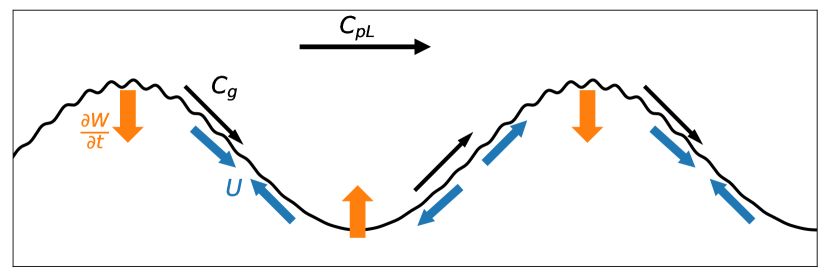
Figure 1: A diagram of short waves riding on longer waves that propagate with their phase-speed $C_{pL}$ from left to right. The short waves propagate on the long-wave surface, their action density moving with the group velocity $C_{g}$. Long waves induce orbital velocities $U$ that cause near-surface convergence and divergence on their front and rear faces, respectively. They also induce downward and upward centripetal accelerations ($\partial W/\partial t$) in the crests and troughs, respectively, that modulate the effective gravity at the surface. As a consequence of surface convergence and divergence and the effective-gravity modulation, the short waves become shorter and higher preferentially on the long-wave crests. The diagram is not to scale.

All modulation solutions mentioned thus far are steady in the reference frame of the long wave—short waves become shorter and higher (and thus, steeper) preferentially on the long-wave crests. Conversely, they elongate and flatten preferentially in the long-wave troughs. Recently, Peureux et al. (2021) asked whether the steady solutions of short-wave modulation are appropriate by simulating the full wave conservation equations. They found that the short waves grow unsteadily due to the propagation of longer waves, suggesting that the steady-state solutions may only be valid for a few long-wave periods before the short waves begin to break due to excessive steepness. However, the unsteadiness of their solutions occurs in a specific scenario in which a long-wave train suddenly appears to modulate a uniform field of short waves. The numerical simulations stabilise if the short-wave field is initialised from existing steady solutions, like those by Longuet-Higgins & Stewart (1960). Nevertheless, their results do put into question whether the short-wave modulation predicted by theory is generally steady over many long-wave periods or not. Looking at the conservation equations alone, it is not obvious that it is.

Reference	Analysis	Gravity	Nonlinear	Nonlinear	Solution
	frameworks	varies	long waves	short waves
Longuet-Higgins & Stewart (1960)	Velocity potential	No	No	No	Analytical
Phillips (1981)	Crest and action	Yes	Yes	No	Numerical
	conservation
Longuet-Higgins (1987)	Velocity potential	Yes	Yes	No	Numerical
Henyey et al. (1988)	Hamiltonian	Yes	Yes	No	Analytical
Zhang & Melville (1990)	Schrödinger	Yes	Yes	Yes	Numerical
Peureux et al. (2021)	Crest and action	Yes	No	No	Numerical
	conservation
This paper	Crest and action	Yes	Yes	No	Analytical
	conservation				and numerical

Table 1: Non-exhaustive summary of prior and present (this paper) approaches to calculating the modulation of short waves by long waves.

In this paper, we revisit this problem from the perspective of linear wave theory but consider the long-wave slope to be significant enough to require evaluating the short-waves at the long-wave surface rather than at the mean water level. This allows us to derive alternative, steady, nonlinear solutions for the modulation of short waves, within the limits of small $\varepsilon_{L}$. The analytical solutions yield modulations that are stronger than the original solution by Longuet-Higgins & Stewart (1960), but similar to the nonlinear numerical solutions by Longuet-Higgins (1987) and Zhang & Melville (1990) in long-wave steepness up to $\approx 0.2$. To validate the steadiness of the analytical solutions, we perform numerical simulations of the full wave crest and action conservation laws, and compare the results to the analytical solutions presented here, as well as the prior numerical results. The numerical simulations are used to determine the validity of the approximate steady solution and to investigate the unsteadiness of the short-wave modulation found by Peureux et al. (2021). The main prior studies on hydrodynamic modulation, and their assumptions and approaches to the solution, are summarised in Table 1. We first present the governing equations in §2, and then the analytical solutions for the modulation of short waves by long waves in §3. Then, we describe the numerical simulations and their results in §4. Finally, we discuss the results and their implications in §5 and conclude the paper in §6.

2 Governing equations

The flow is inviscid, irrotational, and incompressible, and without sources or sinks. In these conditions, linear, deep-water, surface gravity waves obey the dispersion relation:

$$\omega=\sqrt{gk}+kU$$ (2)

where $\omega$ is the angular frequency in a fixed reference frame, $g$ is the gravitational acceleration, $k$ is the wavenumber, and $U$ is the mean advective current in the direction of the wave propagation. A current in the direction of the waves increases their absolute frequency without changing their wavenumber. An important limitation here is that $U$ must be slowly varying on the scales of the wave period (Bretherton & Garrett, 1968). From the perspective of short waves riding on long waves, the advective current is the horizontal near-surface orbital velocity of the long wave. Strictly, a velocity profile must be considered when determining the advective velocity for a wave of any given wavenumber (Stewart & Joy, 1974), however for brevity here we will assume a surface velocity to be the advective one for short waves. The evolution of the short-wave wavenumber is described by the conservation of wave crests (Phillips, 1981):

$$\dfrac{\partial k}{\partial t}+\dfrac{\partial\omega}{\partial x}=0$$ (3)

where $t$ and $x$ are time and space, respectively. This relation states that the wavenumber must change locally when the frequency varies in space.

(2) and (3) describe the evolution of the short-wave wavenumber. To describe the evolution of the wave amplitude, use the wave action balance (Bretherton & Garrett, 1968) in absence of sources (e.g. due to wind) and sinks (e.g. due to whitecapping):

$$\dfrac{\partial N}{\partial t}+\dfrac{\partial}{\partial x}\left[\left(C_{g}+U\right)N\right]=0$$ (4)

where $N$ is the action density of short waves defined as the ratio of their energy density to their intrinsic frequency, $E/\sigma$, and $C_{g}=1/2\sqrt{g/k}$ is their group speed in deep water. The wave action density expressed as $E/\sigma$ is commonly taken as conservative in wave modulation theory (Phillips, 1981; Longuet-Higgins, 1987), however as Dysthe et al. (1988) show, it is conservative only for gently sloped waves. Although the absence of wave growth and dissipation is not generally realistic in the open ocean, it is a useful approximation here to isolate the effects of hydrodynamic modulation solely due to the motion of the long waves.

Short waves that ride on the surface of the longer waves move in an accelerated reference frame (due to the centripetal acceleration at the long-wave surface) and thus experience effective gravitational acceleration that varies in space and time (Phillips, 1981; Longuet-Higgins, 1986, 1987). Inserting (2) into (3) and noting that:

$$\dfrac{\partial\sqrt{gk}}{\partial x}=\dfrac{1}{2}\sqrt{\dfrac{g}{k}}\dfrac{\partial k}{\partial x}+\dfrac{1}{2}\sqrt{\dfrac{k}{g}}\dfrac{\partial g}{\partial x}$$ (5)

we get:

$$\dfrac{\partial k}{\partial t}+\left(C_{g}+U\right)\dfrac{\partial k}{\partial x}+k\dfrac{\partial U}{\partial x}+\dfrac{1}{2}\sqrt{\dfrac{k}{g}}\dfrac{\partial g}{\partial x}=0$$ (6)

From left to right, the terms in this equation represent the change in wavenumber due to the propagation and advection by ambient current $U$, the convergence of the ambient current, and the spatial inhomogeneity of the gravitational acceleration. In a non-accelerated reference frame (i.e. in absence of longer waves), the last term vanishes. It is otherwise necessary to conserve the wave crests.

For the wave action, expand (4) to get:

$$\dfrac{\partial N}{\partial t}+\left(C_{g}+U\right)\dfrac{\partial N}{\partial x}+N\dfrac{\partial U}{\partial x}+N\dfrac{\partial C_{g}}{\partial x}=0$$ (7)

This equation is similar to (6), except for the last term which represents the inhomogeneity of the group speed. As Peureux et al. (2021) explained, the presence of this term causes unsteady growth of wave action in infinite long-wave trains. (6) and (7) are the governing equations that we approximate and solve analytically in §3, and numerically in their full form in §4. It is worth noting that this system of equations is semi-coupled, meaning that it is possible to solve (6) on its own, but solving (7) requires also the solution of (6). In other words, the wave kinematics (the wavenumber distribution) are not concerned with the wave action. In contrast, the wave action is governed, among others, by the group velocity and thus depends on the wavenumber.

For the ambient forcing, we consider a train of monochromatic long waves defined, to the first order in $\varepsilon_{L}$, by the elevation $\eta_{L}=a_{L}\cos{\psi}$, where $\psi=k_{L}x-\sigma_{L}t$ is the long-wave phase and $\sigma_{L}$ its angular frequency. The velocity potential of the long wave is:

$$\phi=\dfrac{a_{L}\omega_{L}}{k_{L}}e^{k_{L}z}\sin{\psi}+\mathcal{O}(\varepsilon_{L}^{4})$$ (8)

where $z$ is the vertical distance from the mean water level that is positive upwards. (8) is accurate to the third order in $\varepsilon_{L}$ in deep water because the second- and third-order terms in the Stokes expansion series are exactly zero. The long-wave induced horizontal and vertical orbital velocities are:

$$U=\frac{\partial\phi}{\partial x}=a_{L}\omega_{L}e^{k_{L}z}\cos{\psi}+\mathcal{O}(\varepsilon_{L}^{4})$$ (9)

$$W=\frac{\partial\phi}{\partial z}=a_{L}\omega_{L}e^{k_{L}z}\sin{\psi}+\mathcal{O}(\varepsilon_{L}^{4})$$ (10)

Evaluating these velocities at the wave surface $z=\eta_{L}$ rather than at the mean water level $z=0$ is a departure from the linear theory, making the treatment of the long waves here as weakly nonlinear. As Zhang & Melville (1990) point out, this is appropriate to do when the amplitude of the long waves is of the similar magnitude or larger than the wavelength of the short waves.

(6)-(7) are the governing equations used in this paper, with (9)-(10) describing the long-wave induced ambient velocity forcing for the short waves. Rather than deriving the modulation solution from the velocity potential of two waves, as Longuet-Higgins & Stewart (1960) did, starting from the crest-action conservation balances allows for a simpler derivation.

3 Analytical solutions

We now describe the analytical solutions for the short-wave wavenumber, effective gravitational acceleration, amplitude, steepness, intrinsic frequency, and intrinsic phase speed in presence of long waves. The wavenumber is derived by linearising the conservation of wave crests (3) and neglecting the spatial gradients of $k$ and $g$. The effective gravity is derived by projecting the long-wave induced surface accelerations onto the local vertical axis (that is, the axis normal to the long-wave surface), akin to Zhang & Melville (1990). The amplitude is derived by first evaluating the short-wave action from the action conservation (4) and then applying the modulated effective gravity to obtain the amplitude. From the modulated wavenumber, amplitude, and effective gravity, the steepness, frequency, and phase speed readily follow from the usual wave relationships. Going forward we will use the tilde over the variables to denote the modulated quantities (e.g. $\widetilde{k}$ for wavenumber).

3.1 Wavenumber modulation

Solving analytically for the wavenumber requires dropping the spatial derivatives of $k$ in (6) and assuming homogeneous $g$:

$$\dfrac{\partial k}{\partial t}=-k\dfrac{\partial U}{\partial x}$$ (11)

Although Peureux et al. (2021) pointed out that the solution by Longuet-Higgins & Stewart (1960) requires assuming homogeneous group speed of the short-wave field, in fact, it also requires assuming no horizontal propagation and advection of the short waves. Combine (9)-(11), and integrate in time to get:

$$\frac{\widetilde{k}}{k}=e^{\varepsilon_{L}\cos{\psi}e^{\varepsilon_{L}\cos{\psi}}}$$ (12)

Notice that the Taylor expansion of (12) to the first order recovers the original solution by Longuet-Higgins & Stewart (1960):

$$\frac{\widetilde{k}}{k}=1+\varepsilon_{L}\cos{\psi}$$ (13)

Coming from the conservation of crests, as opposed to the velocity potential superposition, the solution by Longuet-Higgins & Stewart (1960) requires two approximations: First, evaluating the long-wave velocity at $z=0$ rather than $z=\eta_{L}$; and second, further truncating the Taylor expansion series beyond the first-order term. These approximations underestimate the short-wave modulation magnitude (Fig. 2a). At the wave crest, (12) yields the wavenumber modulation that is 16.9%, 38.5%, 66.4%, and 104% larger than that of Longuet-Higgins & Stewart (1960) for $\varepsilon_{L}=0.1,0.2,0.3,0.4$, respectively. Although not immediately obvious from the expressions, the modulated wavenumber (13) is conserved across the long-wave phase, whereas the higher-order solution (12) is not. This is because combining the orbital velocities evaluated at $z=\eta_{L}$ and the linearised conservation of wave crests in (6) creates excess short-wave wavenumber. The solution of (6) must be conservative across the long-wave phase, as we will see later from the numerical simulations.

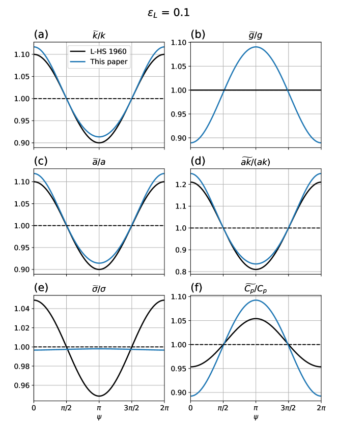
Figure 2: Steady solutions for the modulation of short-wave (a) wavenumber, (b) gravitational acceleration, (c) amplitude, (d) steepness, (e) intrinsic frequency, and (f) intrinsic phase speed as function of long-wave phase for $\varepsilon_{L}=0.1$, based on Longuet-Higgins & Stewart (1960) (L-HS 1960, black) and this paper (blue). Long-wave crest and trough are located at $\psi=0$ and $\psi=\pi$, respectively.

3.2 Gravity modulation

Long waves induce orbital (centripetal) accelerations on their surface, so the short waves ride in an accelerated reference frame and experience effective gravity that is lower at the crests and higher in the troughs (Longuet-Higgins, 1986, 1987). Further, the projection of the long-wave induced horizontal acceleration contributes to small but non-negligible effects on the short-wave effective gravity in the curvilinear coordinate system (Phillips, 1981; Zhang & Melville, 1990). These two effects are completely described by projecting the gravitational acceleration vector from the coordinate that is perpendicular to the mean water surface ($z=0$) to that which is perpendicular to the long-wave surface ($z=\eta_{L}$), and likewise for the long-wave orbital accelerations:

$$\frac{\widetilde{g}}{g}=\cos{\alpha}+\dfrac{\partial W_{z=\eta}}{\partial t}\cos{\alpha}+\dfrac{\partial U_{z=\eta}}{\partial t}\sin{\alpha}$$ (14)

$$\alpha=\tan^{-1}{\dfrac{\partial\eta}{\partial x}}$$ (15)

where $\alpha$ is the local slope of the long-wave surface. For short waves on a linear long wave, the gravity modulation is:

$$\frac{\widetilde{g}}{g}=\frac{1-\varepsilon_{L}\cos{\psi}e^{\varepsilon_{L}\cos{\psi}}\left[1+\left(\varepsilon_{L}\sin{\psi}\right)^{2}\right]}{\sqrt{\left(\varepsilon_{L}\sin{\psi}\right)^{2}+1}}$$ (16)

Curvilinear effects on effective gravity can be removed altogether by setting $\alpha=0$. In that case, (14) simplifies to:

$$\frac{\widetilde{g}}{g}=1-\varepsilon_{L}\cos{\psi}e^{\varepsilon_{L}\cos{\psi}}$$ (17)

If we evaluate the orbital accelerations at the mean water level $z=0$, this further simplifies to:

$$\frac{\widetilde{g}}{g}=1-\varepsilon_{L}\cos{\psi}$$ (18)

which is the form used by Peureux et al. (2021), for example.

The general form of the gravity modulation (14) is convenient because it allows us to easily attribute the modulation to different processes. It also makes it straightforward to evaluate the gravity modulation for a different long-wave form, by evaluating the orbital accelerations and the local slope for that wave. For a third-order Stokes wave, for example, the elevation is:

$$\eta_{St}=a_{L}\left[\cos{\psi}+\dfrac{1}{2}\varepsilon_{L}\cos{2\psi}+\varepsilon_{L}^{2}\left(\dfrac{3}{8}\cos{3\psi}-\dfrac{1}{16}\cos{\psi}\right)\right]+\mathcal{O}(\varepsilon_{L}^{4})$$ (19)

Without considering the curvilinear effects in (14), the gravitational acceleration at the surface of a Stokes wave is, to the third order:

$$\frac{\widetilde{g}}{g}=\left\{1-\varepsilon_{L}e^{k\eta_{St}}\left[\cos{\psi}-\varepsilon_{L}\sin{\psi}\left(\sin{\psi}+\varepsilon_{L}\sin{2\psi}-\dfrac{1}{16}\varepsilon_{L}^{2}\sin{\psi}+\dfrac{9}{8}\varepsilon_{L}^{2}\sin{3\psi}\right)\right]\right\}$$ (20)

The equivalent expression that includes the curvilinear effects can be derived by evaluating the velocities and the local slope $\alpha$ at $z=\eta_{St}$, and inserting them into (14):

$$\frac{\widetilde{g}}{g}=\cos{\alpha_{St}}+\dfrac{\partial W_{z=\eta_{St}}}{\partial t}\cos{\alpha_{St}}+\dfrac{\partial U_{z=\eta_{St}}}{\partial t}\sin{\alpha_{St}}$$ (21)

$$\alpha_{St}=\tan^{-1}{\dfrac{\partial\eta_{St}}{\partial x}}$$ (22)

Let us now examine the contributions of the different terms to the short-wave effective gravity modulation. Fig. 3a shows the effective gravity modulation of short-wave as a function of the long-wave phase for $\varepsilon_{L}=0.2$, for a variety of the gravity modulation forms. This value of $\varepsilon_{L}$ allows easier visualisation of the modulation differences, while still being relatively moderate. To the first order in $\varepsilon_{L}$, the gravity modulation is out of phase with the long-wave elevation, with the short waves experiencing a lower effective gravity on the long-wave crests and a higher effective gravity in the troughs. Evaluating the orbital accelerations at $z=\eta_{L}$ causes a gravity reduction around the crests ($\approx 6\%$) and the troughs ($\approx 3\%$), and an increase on the front and rear faces ($\approx 4\%$) of the long wave, due to the exponential change in the orbital accelerations away from the mean water level (Fig. 3b). The difference between the linear and Stokes long waves at this steepness is negligible. The long-wave elevation curvature has a second-order effect in $\varepsilon_{L}$. Naturally, there is no curvature exactly at the crests and the troughs, and its effects are largest at the front and rear faces of the long wave, where the covariance between the local slope and the horizontal accelerations are largest.

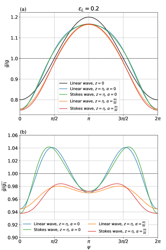
Figure 3: (a) Analytical solutions for the effective gravitational acceleration modulation by long waves, as function of long-wave phase, for $\varepsilon_{L}=0.2$. Black is for linear wave evaluated at $z=0$, blue and green are for linear and Stokes waves, respectively, evaluated at $z=\eta$ and without curvature effects, and orange and green are for linear and Stokes waves, respectively, evaluated at $z=\eta$ and with curvature effects. (b) As in (a) but normalised by the modulation of the linear wave evaluated at $z=0$, $g_{1}$.

It is instructive to also examine the mean, maximum, and minimum values of the effective gravity as function of long-wave steepness $\varepsilon_{L}$ (Fig. 4). The long-wave averaged effective gravity of short waves remains equal to the resting value of $g$ for all values of $\varepsilon_{L}$, except if the effects of curvature are considered, in which case the average effective gravity is reduced. This reduction, in case of a long Stokes wave, is $\approx 3\%$ for $\varepsilon_{L}=0.2$ and $\approx 14\%$ for $\varepsilon_{L}=0.4$. As the effective gravity minima and maxima occur at crests and troughs, respectively, the curvature affects the phase-averaged values but not the extremes. As the slope effects on the effective gravity exist only away from crests and troughs, they may be neglected in the steady solutions where modulation is typically evaluated at the long-wave crests. The effective gravity reduction at the crests is $\approx 11\%$, $25\%$, and $66\%$ for $\varepsilon_{L}=0.1$, $0.2$, and $0.4$, respectively. These are similar to the fully-nonlinear numerical estimates of Longuet-Higgins (1986, 1987). Note that these are strictly Eulerian values, evaluated at fixed positions in space. As Longuet-Higgins (1986) pointed out, the effective gravity in the Lagrangian frame (i.e., following the surface particles) is smoother and less amplified because the moving particles spend a longer time riding near the crests and less time returning through the troughs. However, when we solve the short-wave crest and action conservation equations in an Eulerian frame, it is the Eulerian effective gravity that must be applied to conserve the short-wave properties across the long-wave phase.

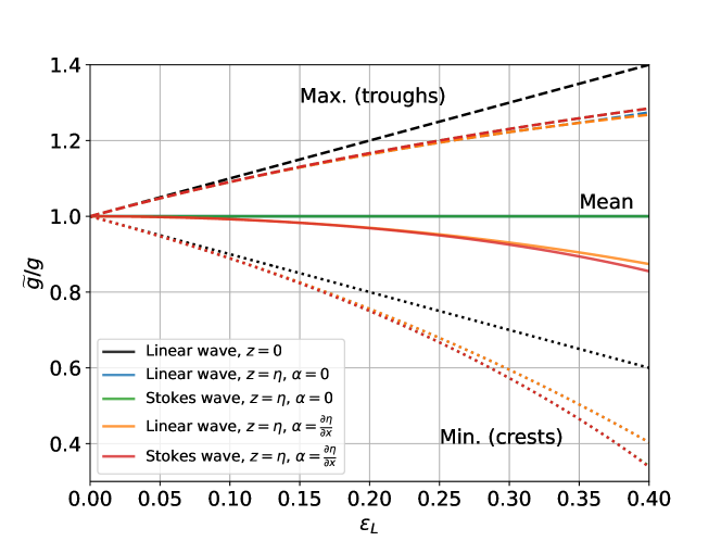
Figure 4: As Fig. 3 but showing the mean (solid), maximum (dashed), and minimum (dotted) short-wave gravity modulation as function of long-wave steepness $\varepsilon_{L}$. The minimum and maximum values for the cases with curvature effects ($\alpha=\frac{\partial\eta}{\partial x}$) are equivalent to those without curvature effects ($\alpha=0$) and obscure them in the plot.

3.3 Amplitude and steepness modulation

The modulation of short-wave amplitude can be derived in a similar way as we did for the wavenumber, except that here we linearise the wave action balance (7) and integrate it in time:

$$\frac{\widetilde{N}}{N}=e^{\varepsilon_{L}\cos{\psi}e^{\varepsilon_{L}\cos{\psi}}}$$ (23)

Since wave action is energy divided by the intrinsic frequency $\sigma$, and energy scales with $ga^{2}$, the modulation of the amplitude is related to the modulations of gravity, wavenumber, and action:

$$\dfrac{\widetilde{a}}{a}=\sqrt{\dfrac{g}{\widetilde{g}}\dfrac{\widetilde{\sigma}}{\sigma}\dfrac{\widetilde{N}}{N}}=\left(\dfrac{\widetilde{k}}{k}\right)^{\frac{1}{4}}\left(\dfrac{\widetilde{N}}{N}\right)^{\frac{1}{2}}\left(\dfrac{g}{\widetilde{g}}\right)^{\frac{1}{4}}$$ (24)

To the first order in $\varepsilon_{L}$, and using (12) and (23), the above simplifies to the result of Longuet-Higgins & Stewart (1960):

$$\dfrac{\widetilde{a}}{a}=\left(\dfrac{g}{\widetilde{g}}\right)^{\frac{1}{4}}\left(1+\varepsilon_{L}\right)^{\frac{3}{4}}\approx\frac{(1+\varepsilon_{L})^{\frac{3}{4}}}{(1-\varepsilon_{L})^{\frac{1}{4}}}\approx 1+\varepsilon_{L}$$ (25)

The amplitude and steepness modulation of the short waves as a function of the long-wave phase for $\varepsilon_{L}=0.1$ are compared to the Longuet-Higgins & Stewart (1960) solutions in Fig. 2 panels (c) and (d), respectively. Also shown are the modulation of the short-wave intrinsic frequency and phase speed in panels (e) and (f), respectively. As the wavenumber and gravity modulations are out of phase, with the latter being somewhat larger in magnitude, the overall intrinsic frequency of the short waves is reduced across the entire long-wave phase, with highest reduction at the long-wave crests. For the short-wave phase speed modulation, the wavenumber and gravity modulations work in tandem and cause the short-wave phase speed to be reduced on the long-wave crests and increased in the troughs. We discuss the implications of this effect later in §5 in the context of wind input to short waves.

Finally, the short-wave steepness modulation follows from (12) and (24):

$$\dfrac{\widetilde{ak}}{ak}=\left(\dfrac{\widetilde{k}}{k}\right)^{\frac{5}{4}}\left(\dfrac{\widetilde{N}}{N}\right)^{\frac{1}{2}}\left(\dfrac{g}{\widetilde{g}}\right)^{\frac{1}{4}}$$ (26)

The short-wave steepness modulation at the long-wave crests is thus largely controlled by the wavenumber modulation (5/8, or, 62.5%), followed by the convergence of wave action (1/4, or, 25%), and by least amount by the effective gravity reduction (1/8, or, 12.5%) (Fig. 5). (26) and Fig. 5 demonstrate that more than half of the steepness modulation can be captured by the wavenumber modulation alone. Further, considering the wavenumber and wave action modulations, while neglecting the gravity modulation, captures $\approx$88% of the steepness modulation at the long-wave crests. This result may be useful for the interpretation of remote sensing products that resolve some but not all of the short-wave modulation effects. Finally, the relative contributions of different modulation factors remain mostly constant as $\varepsilon_{L}$ increases, with only a mild increase of the effective gravity modulation contribution, and mild increases of the wavenumber and wave action modulation contributions.

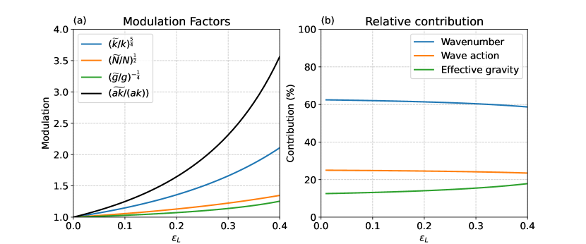
Figure 5: Contributions of short-wave wavenumber, action, and effective gravity modulations to the steepness modulation, as function of the long-wave steepness $\varepsilon_{L}$. Panel (a) shows each modulation factor (colour) and their product (black), and panel (b) shows their relative contributions in percentage, calculated as the ratio of the logarithm of each modulation factor to the logarithm of the product of all modulations.

4 Numerical solutions

4.1 Model description

To quantify the contribution of the nonlinear terms in (6) and (7), and to evaluate the steadiness assumption of the analytical solutions, we now proceed to numerically integrate the full set of crest and action conservation equations. (6) and (7) are discretised using second-order central finite difference in space and integrated in time using the fourth-order Runge-Kutta method (Butcher & Wanner, 1996). The space is divided into 100 grid points. This is effectively the same equation set and numerical configuration as that of Peureux et al. (2021), except that their long-wave orbital velocities are evaluated at $z=0$ instead of $z=\eta_{L}$, thus neglecting the Stokes drift induced by long waves on short-wave groups (Stokes, 1847; van den Bremer & Breivik, 2018; Monismith, 2020). Their gravity modulation also does not consider the nonlinear or the curvature effects, however, this difference does not qualitatively affect the results. Another difference is the choice of the numerical scheme for spatial differences, which in their case is the more sophisticated MUSCL4 scheme (Kurganov & Tadmor, 2000). Although the second-order central finite difference is not appropriate for many numerical problems, in our case it is sufficient because it is conservative and the fields that we compute derivatives of are smooth and continuous. The maximum relative error of the centred finite difference in this model is $\approx 0.066\%$. The wavenumber and wave action are conservative over time within $\mathcal{O}(10^{-7})$ and $\mathcal{O}(10^{-5})$ relative error, respectively. We show in the next section that our numerical solutions for infinite long-wave trains are qualitatively equivalent to those of Peureux et al. (2021).

The numerical equations here are integrated in a fixed reference frame, rather than that moving with the long-wave phase speed. Either approach produces equivalent modulation results, however a fixed reference frame may allow for a more intuitive interpretation of the results. This difference is important to keep in mind when comparing the results of Peureux et al. (2021) and those presented here; in their Fig. 1 the long-wave phase is fixed and the short waves are moving leftward with the speed of $C_{pL}-C_{g}-U$ (neglecting group speed inhomogeneity), whereas in the figures that follow, the long wave is moving rightward with its phase speed $C_{pL}$ and the short waves (that is, their action) are moving rightward with the speed of $C_{g}+U$ (neglecting group speed inhomogeneity). The crest and action conservation equations are integrated in the curvilinear coordinate system in which the horizontal coordinate follows the long-wave surface, akin to Zhang & Melville (1990).

4.2 Comparison with analytical solutions

The first set of simulations is performed for the long-wave steepness of $\varepsilon_{L}=0.1$, $0.2$, and $0.4$ (Fig. 6). The long-waves are initialised from rest ($a_{L}=0$) and gradually ramped up to their target steepness over 5 long-wave periods, thus emulating the passage of a long-wave group (the importance of which we discuss in more detail in the next subsection). At $\varepsilon=0.1$, the numerical solutions for the wavenumber, amplitude, and steepness modulation are all remarkably similar to the analytical solutions (Fig. 6a,d,g). This suggests that at low long-wave steepness that the steady analytical solution is a reasonable proxy for the fully-nonlinear crest-action conservation equation solutions. The numerical solutions diverge more notably from the analytical ones at moderate steepness of 0.2 (Fig. 6b,e,h), and are considerably different at very high steepness of 0.4 (Fig. 6c,f,i). These differences suggest that at high steepness the inhomogeneity of gravitational acceleration and group speed, otherwise ignored in the steady solutions, become important.

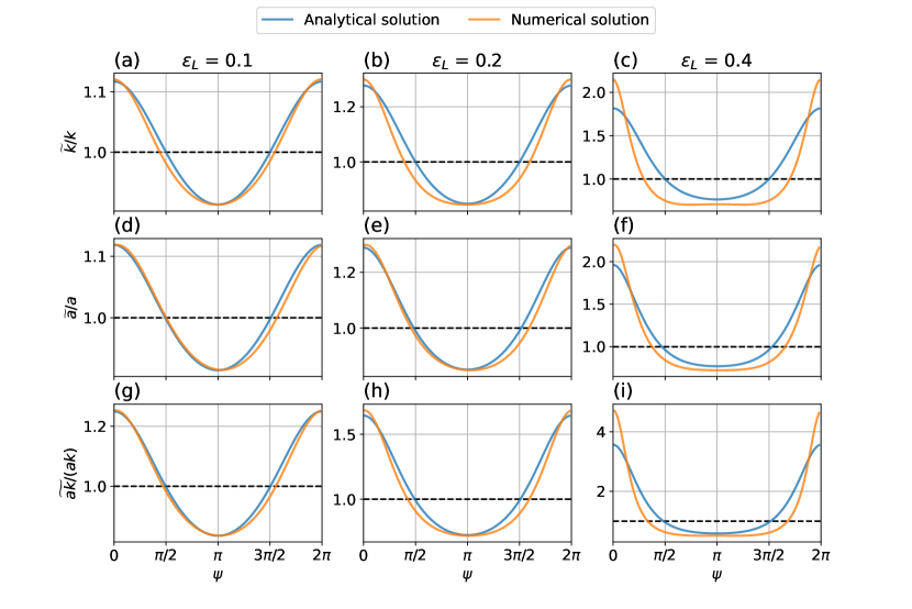
Figure 6: Comparison of numerical solutions (orange) of wavenumber (top), amplitude (middle), and steepness (bottom) modulation with their analytical solutions (blue), for $\varepsilon_{L}$ = 0.1, 0.2, and 0.4.

The maximum modulations of the short-wave wavenumber, amplitude, and steepness from the analytical and numerical solutions, are shown on Figs. 7, 8, and 9, respectively, as function of the long-wave steepness $\varepsilon_{L}$. Overall, the numerical solutions, based on the linear and the third-order Stokes long waves alike, begin to diverge from the analytical solution at $\varepsilon_{L}\approx 0.2$. The numerical solution using the Stokes long wave is quantitatively very similar to the fully-nonlinear solutions of Longuet-Higgins (1987) in amplitude modulation, however with somewhat lower wavenumber and steepness modulations. For example, at $\varepsilon_{L}=0.4$, the steepness modulation in our solutions is close to 6, whereas Longuet-Higgins (1987) finds it close to 8. The underestimate in the wavenumber modulation at high long-wave steepness relative to the results of Longuet-Higgins (1987) is likely due to his long wave velocities being evaluated to a higher order in $\varepsilon_{L}$ than they are here. Nevertheless, the overall steepness modulation between the two numerical approaches are remarkably similar, and either solution would cause the short-waves of even low steepness to break (Banner & Peregrine, 1993). Where the two modulation solutions differ (at $\varepsilon_{L}>0.2$), either solution would lead to short-wave breaking after one long-wave period. This suggests that in the cases where the short-waves would survive the modulation and persist over multiple long-wave periods, the two solutions are effectively equivalent.

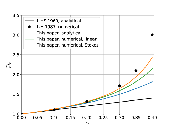
Figure 7: Maximum wavenumber modulation as function of long-wave steepness $\varepsilon_{L}$. Black line and circles are for the analytical and numerical solutions from Longuet-Higgins & Stewart (1960) and Longuet-Higgins (1987), respectively. Blue line is based on the analytical solutions from this paper. Green and orange lines are for the numerical solutions from this paper using linear and third-order Stokes long waves, respectively.

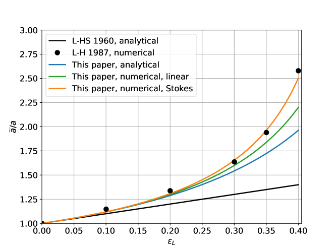
Figure 8: As Fig. 7 but for the amplitude modulation.

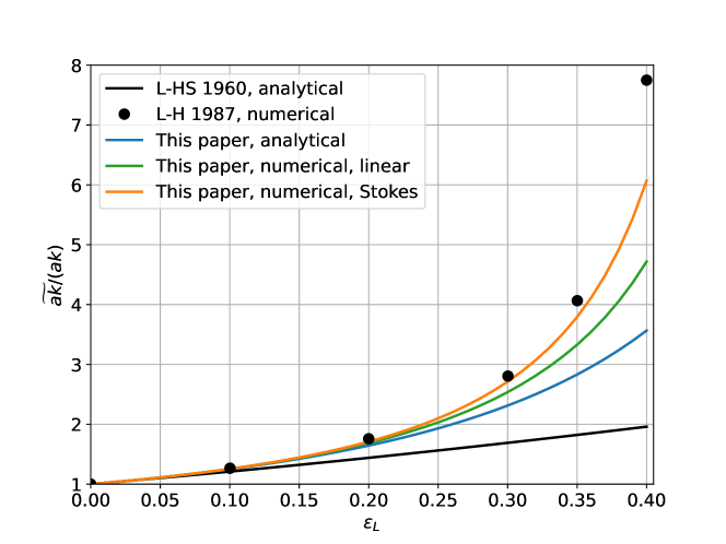
Figure 9: As Fig. 7 but for the steepness modulation.

4.3 Unsteady growth in Pereux et al. (2021)

The key result of Peureux et al. (2021) is that of unsteady steepening of short waves when a homogeneous field of short waves is forced by an infinite long-wave train. The steepening is driven by the progressive increase in the action of short waves (as opposed to their wavenumber), and is centred on the short-wave group that begins its journey in the trough of the long wave. This is because the unmodulated short waves that begin their journey in the trough first enter the convergence region before reaching the divergence region. Inversely, the short waves that begin around the crest of the long-wave first enter the divergence region and will thus have their action and wavenumber decreased. We reproduce this behaviour in Fig. 10, which shows the evolution of the short-wave action, wavenumber, and steepness modulation (here defined as the change of a quantity relative to its initial value). The long waves have $\varepsilon_{L}=0.1$ and $k_{L}=1$, and the short waves have $k=10$. After 10 long-wave periods, the short-wave action is approximately doubled, consistent with Peureux et al. (2021). Another important property of this solution is that the short-wave group that experiences peak amplification (dampening) are not locked-in to the long-wave crests (troughs), as they are in the prior steady solutions (Longuet-Higgins & Stewart, 1960; Longuet-Higgins, 1987; Zhang & Melville, 1990).

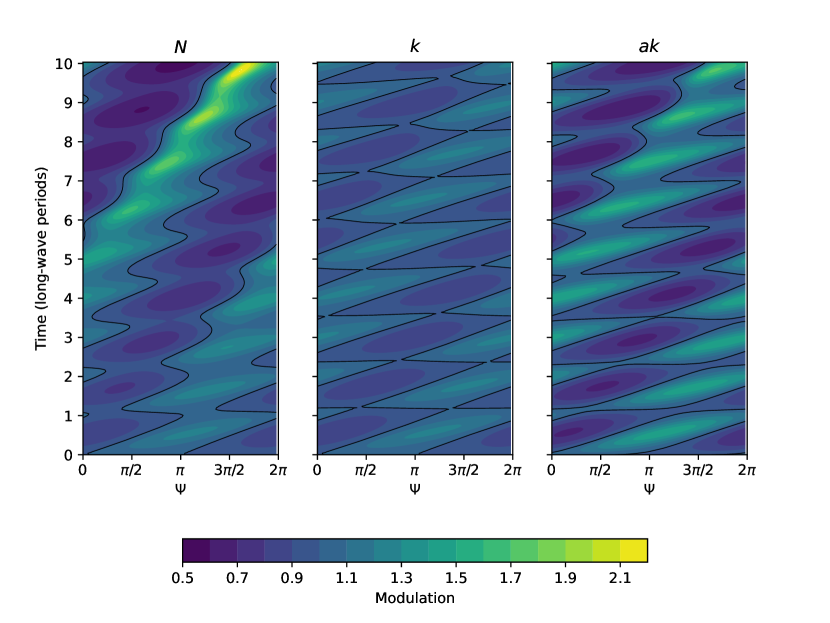
Figure 10: Change in the short-wave action (left), wavenumber (middle), and steepness (right) relative to their initial values as function of initial long-wave phase and time. $k_{L}=1$, $k=10$, $\varepsilon_{L}=0.1$. The black contour follows the value of 1, which corresponds to no change from the initial values.

Why does this unsteady growth of short-wave action occur? Peureux et al. (2021) explain that the change in advection velocity due to the modulation of the short-wave group speed yields an additional amplification of the short-wave action. That is, the inhomogeneity term $N\partial C_{g}/\partial x$ is responsible for the instability. However, the instability only occurs if the short waves are initialised as a uniform field. If they are initialised instead as a periodic function of the long-wave phase such that their wavenumber (and optionally, action) is higher on the crests and lower in the troughs, akin to the prior steady solutions, the instability vanishes and the short-wave modulation pattern locks-in to the long-wave crests.

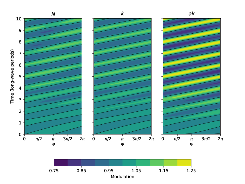
Figure 11: Same as Fig. 10 but with a linear ramp applied to $a_{L}$ during the initial five long-wave periods.

Why is it, then, that the solution for short-wave modulation is not only quantitatively, but also qualitatively, different depending on the short-wave initial conditions? It may at first seem that there is something special about the uniform initial conditions that makes its solutions grow unsteadily and indefinitely. Peureux et al. (2021) described this scenario as ”…the sudden appearance of a long wave perturbation in the middle of a homogeneous short wave field”. However, it is not obvious whether such a scenario is realistic as waves tend to disperse into groups, and the time scales of incoming swell fronts are much longer than those of short-wave generation by wind. To test whether the sudden onset of long-wave forcing causes the unsteady growth, we repeat the numerical simulation of Fig. 10, except for a linear ramp applied to $a_{L}$ (and consequently, the other long-wave properties including the orbital velocities and the local steepness) for the first five periods: $a_{L}(t)=min(a_{L},a_{L}t/\left(5T_{L}\right))$, where $T_{L}$ is the long-wave period. This result is shown in Fig. 11. The key distinction that arises with the introduction of the ramp is that the modulation pattern of short waves is now locked-in to the long-wave crests, and their indefinite steepening vanishes. The stabilisation effect of the long-wave ramp is more readily assessed in Fig. 12, which shows the maximum short-wave steepness modulation as function of time over 30 long-wave periods, for the infinite long-wave train case and the case of applying a linear ramp. Comparing the wave action propagation ($C_{g}\partial N/\partial x$) and inhomogeneity ($N\partial C_{g}/\partial x$) tendencies reveals that after only one long-wave period, the propagation and inhomogeneity tendencies are unbalanced and amplify the steepening of short waves (Fig. 13). Peureux et al. (2021) correctly pointed out that the unsteady growth of short-wave steepness occurs due to the resonance of the inhomogeneity tendency with the short-wave action perturbation. However, in the case of a gentle ramp-up of the long-wave forcing, the propagation and inhomogeneity tendencies mostly balance each other and allow the short-wave steepening to lock-in to the long-wave crests.

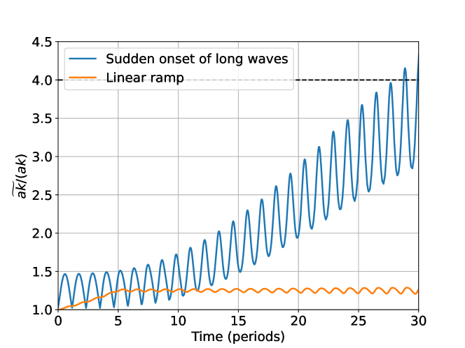
Figure 12: Maximum short-wave steepness modulation as function of time in case of infinite long-wave train case (blue) and the same case but with a linear ramp during the initial five long-wave periods (orange). The dashed black line corresponds to the short-wave steepness of 0.4 at which most waves are expected to break.

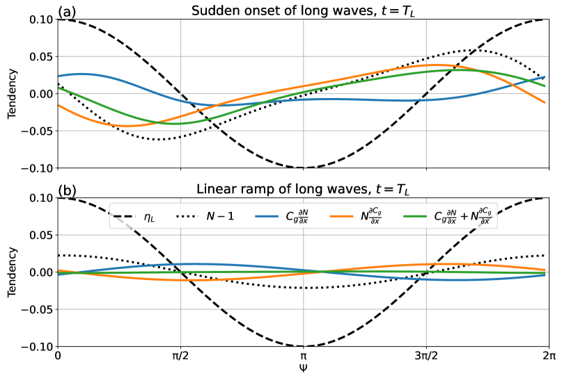
Figure 13: Propagation ($C_{g}\frac{\partial N}{\partial x}$) (blue) and inhomogeneity ($N\frac{\partial C_{g}}{\partial x}$) (orange) tendencies and their sum (green) for the short-wave action after one long-wave period, in the case of (a) infinite long-wave train and (b) linear ramp of long-wave amplitude. Dashed line is the long-wave elevation and the dotted line is the short-wave action modulation minus 1.

4.4 Short-wave modulation by long-wave groups

We now proceed to examine the numerical solutions with the long-wave forcing applied as a long-wave group. The wave group is simulated as a non-dispersive train of long waves whose amplitude scales with $\sin[\pi t/(nT_{L})]$, where $n$ is the number of long waves in the group. The elevation of the long waves thus gradually ramps up from rest to $a_{L}$ at $t=nT_{L}/2$, after which it gradually decreases toward zero. In this simulation, $n=10$ and $\varepsilon_{L}=0.1$ as in the previous two simulations. The modulations of short-wave wavenumber, amplitude, and steepness in response to such long-wave group is shown in Fig. 14. Like in the case of a linear ramp, the modulation pattern here is locked in to the long-wave crest and peaks at approximately 1.2 for short-wave steepness. After the peak of the long-wave group passes, the short-wave modulation recedes back toward the resting state.

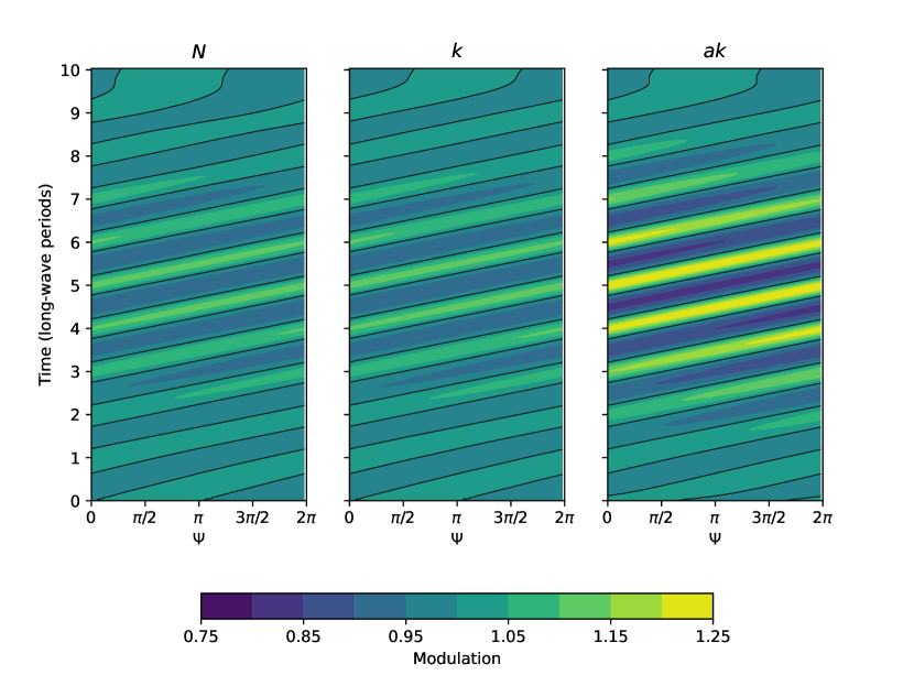
Figure 14: Same as Fig. 10 but for a long-wave group, causing the long-wave amplitude to gradually increase and peak at $a_{L}=0.1$ after five long-wave periods, and then conversely decay back to a calm sea state.

5 Discussion

The solutions presented here, analytical and numerical alike, are valid only for certain scales of short and long waves. Specifically, the wave action conservation equation, introduced by Bretherton & Garrett (1968), requires that the ambient velocity is slowly varying on the time scales of short waves, i.e. $|\partial U/\partial x|\ll k|U|$ and $|\partial U/\partial t|\ll\sigma|U|$. This implies $k_{L}\ll k$ and $\sigma_{L}\ll\sigma$, respectively. Another requirement is for the short-waves to remain linear, which implies $ak\ll 1$. Furthermore, the short waves examined here do not include the effects of surface tension (gravity-capillary waves) or intermediate or shallow water, although the solutions can be extended to those conditions, as Phillips (1981) did, for example. Within these limits, the crest-action conservation equations provide an elegant and relatively simple framework to study the hydrodynamic modulation of short waves by longer waves. This approach, of course, isolates this particular process from other dominant modulation and nonlinear transfer processes, such as wave growth by wind, wave dissipation, and aerodynamic sheltering by the longer waves, that are otherwise present in most measurements (Plant, 1986; Laxague et al., 2017).

Although in this paper we only explored the solutions for $k_{L}=1$ and $k=10$ the results are not sensitive to different values of $k_{L}$, provided the same long-wave steepness $\varepsilon_{L}=a_{L}k_{L}$. Numerical simulations with $k/k_{L}=10$ and $k/k_{L}=100$ show little sensitivity to the ratio $k/k_{L}$ (not shown), consistent with the results of Longuet-Higgins (1987). Specifically, the short-wave steepness modulation is 1% larger at $\varepsilon_{L}=0.27$ for $k/k_{L}=10$ compared to $k/k_{L}=100$, and 4% larger at $\varepsilon_{L}=0.4$. This suggests that as long as $k/k_{L}\gg 1$, the modulation amplitude is largely independent of the ratio $k/k_{L}$. These results can be reproduced with the companion numerical model. Also not considered here are the short-wave trains that are oblique to the longer waves, which is relatively straightforward to include (Peureux et al., 2021).

Despite several studies that provided qualitatively similar steady solutions for the short-wave modulation by long waves (Longuet-Higgins & Stewart, 1960; Phillips, 1981; Longuet-Higgins, 1987; Henyey et al., 1988; Zhang & Melville, 1990), it was not obvious from the governing equations that the fully-nonlinear steady solutions should exist. Peureux et al. (2021) examined this problem numerically and found that the solutions are stable only if the short-wave field is initialised from a prior steady solution of the form of that from Longuet-Higgins & Stewart (1960). If the short-wave field is instead initialised from a uniform field, they found that the short-wave amplitude, and thus steepness as well, grow unsteadily. However, here we demonstrate that the unsteady steepening of short waves only occurs in the case of a sudden appearance of long waves, where the velocity fields induced by the long waves act in their full capacity on the short waves that have not yet had time to lock-in to the long-wave crests. In such a scenario, sudden forcing on short waves causes the modulation pattern to detach itself from the long-wave crests and to propagate at the short-wave group speed. When this occurs, the modulated short-waves are no longer in a stabilising resonance with the surface convergence and divergence induced by the long-wave orbital velocity, and each long-wave passage further destabilises the short-wave field, causing it to steepen indefinitely.

Another important consideration of the hydrodynamic modulation process is whether it should somehow be accounted for in phase-averaged spectral wave models (WAMDI Group, 1988; Tolman, 1991; Donelan et al., 2012) used for global and regional wave forecasting. Currently, most spectral wave models used for research or forecasting do not consider the preferential steepening of short waves in the context of their dispersion properties or the wind input via the short-wave phase speed. Some dissipation source functions use the cumulative mean squared slope to quantify preferential dissipation of short waves due to this effect (Donelan et al., 2012; Romero, 2019). In the early days of spectral wave modelling, Willebrand (1975) examined the effect of a wave spectrum on the short-wave group velocity and found the modulation effect to be up to several percent. For a practical implementation, this would incur an additional loop over all frequencies longer than the considered short-wave frequency. It was thus not deemed practical to include this effect in wave models at the time. However, with the recent advances in computing power, machine learning for acceleration of complex functions, and phase-resolved modelling of short waves, considering the effect of wave-modulation beyond the simple cumulative mean squared slope deserves re-examination.

6 Conclusions

In this paper we revisited the problem of short-wave modulation by long waves from a linear wave theory perspective. Using the linearised wave crest and action conservation equations coupled with nonlinear solutions for the effective gravity, we derived steady analytical solutions for the modulation of short wave wavenumber, amplitude, steepness, intrinsic frequency, and phase speed. The latter two have not been previously examined in the context of short-wave modulation, but may be important for correctly calculating the wind input into short waves, which is proportional to the wind speed relative to the wave celerity. The approximate steady solutions yield higher wavenumber and amplitude modulation than that of Longuet-Higgins & Stewart (1960), and somewhat lower than the numerical solutions of Longuet-Higgins (1987) and Zhang & Melville (1990). This is mainly due to the analytical solution requiring the crest and action conservation equations to be linearised, and the nonlinearity arising due to the evaluation of short waves on the surface of the long wave (as opposed to the mean water level) and due to nonlinear effective gravity. In the steady solutions, the short-wave steepness modulation is dominated by the wavenumber modulation (5/8), followed by the wave action modulation (1/4), and is least affected by the effective gravity modulation (1/8).

The numerical solutions of the full wave crest and action conservation equations are consistent with the analytical solutions for $\varepsilon_{L}\lesssim 0.2$, and are similar in amplitude to the numerical solutions of Longuet-Higgins (1987) and Zhang & Melville (1990). The simulations also reveal that the unsteady growth of short-wave steepness reported by Peureux et al. (2021) is due to the sudden appearance of long waves in a homogeneous short-wave field, a scenario that is unlikely to occur in the open ocean. A more likely condition such as that of long-wave groups, are only mildly destabilising for the short waves. These results suggest that for mildly-to-moderately steep short waves, the analytical steady solutions presented here are sufficient to describe the modulation of short waves by long waves. It may be worthwhile to revisit a more systematic inclusion of the hydrodynamic modulation effects in phase-averaged spectral wave models, beyond the simple cumulative mean squared slope for wave dissipation, but also for modulating the dispersion and wind input into short waves.

[Acknowledgements] I am thankful to Nathan Laxague, Fabrice Ardhuin, Nick Pizzo, and Peisen Tan for the discussions that helped improve this paper.

[Funding] Milan Curcic was partly supported by the National Science Foundation grant AGS-1745384, Transatlantic Research Partnership by the French Embassy in the United States and the FACE Foundation, and the Office of Naval Research Coastal Land Air-Sea Interaction DRI.

[Declaration of interests]The author reports no conflict of interest.

[Data availability statement] The code to run the numerical simulations and generate the figures in this paper is available at https://github.com/wavesgroup/wave-modulation-paper. The numerical model is available as a standalone Python package at https://github.com/wavesgroup/2wave.

[Author ORCIDs]M. Curcic, https://orcid.org/0000-0002-8822-7749

References

- Banner & Peregrine (1993) Banner, ML & Peregrine, DH 1993 Wave breaking in deep water. Annual review of fluid mechanics 25 (1), 373–397.
- Belcher (1999) Belcher, SE 1999 Wave growth by non-separated sheltering. European Journal of Mechanics-B/Fluids 18 (3), 447–462.
- van den Bremer & Breivik (2018) van den Bremer, Ton S & Breivik, Øyvind 2018 Stokes drift. Philosophical Transactions of the Royal Society A: Mathematical, Physical and Engineering Sciences 376 (2111), 20170104.
- Bretherton & Garrett (1968) Bretherton, Francis P & Garrett, Christopher John Raymond 1968 Wavetrains in inhomogeneous moving media. Proceedings of the Royal Society of London. Series A. Mathematical and Physical Sciences 302 (1471), 529–554.
- Butcher & Wanner (1996) Butcher, John Charles & Wanner, Gerhard 1996 Runge-kutta methods: some historical notes. Applied Numerical Mathematics 22 (1-3), 113–151.
- Chen & Belcher (2000) Chen, Gang & Belcher, Stephen E 2000 Effects of long waves on wind-generated waves. Journal of Physical Oceanography 30 (9), 2246–2256.
- Donelan et al. (2012) Donelan, MA, Curcic, M, Chen, SS & Magnusson, AK 2012 Modeling waves and wind stress. Journal of Geophysical Research: Oceans 117 (C11).
- Donelan (1987) Donelan, Mark A 1987 The effect of swell on the growth of wind waves. Johns Hopkins APL Technical Digest 8 (1), 18–23.
- Dysthe et al. (1988) Dysthe, K, Henyey, FS, Longuet-Higgins, Michael Selwyn & Schult, RL 1988 The orbiting double pendulum: an analogue to interacting gravity waves. Proceedings of the Royal Society of London. A. Mathematical and Physical Sciences 418 (1855), 281–299.
- Hara & Plant (1994) Hara, Tetsu & Plant, William J 1994 Hydrodynamic modulation of short wind-wave spectra by long waves and its measurement using microwave backscatter. Journal of Geophysical Research: Oceans 99 (C5), 9767–9784.
- Henyey et al. (1988) Henyey, Frank S., Creamer, Dennis B., Dysthe, Kristian B., Schult, Roy L. & Wright, Jon A. 1988 The energy and action of small waves riding on large waves. Journal of Fluid Mechanics 189, 443–462.
- Keller & Wright (1975) Keller, WC & Wright, JW 1975 Microwave scattering and the straining of wind-generated waves. Radio science 10 (2), 139–147.
- Kurganov & Tadmor (2000) Kurganov, Alexander & Tadmor, Eitan 2000 New high-resolution central schemes for nonlinear conservation laws and convection–diffusion equations. Journal of computational physics 160 (1), 241–282.
- Laxague et al. (2017) Laxague, Nathan JM, Curcic, Milan, Björkqvist, Jan-Victor & Haus, Brian K 2017 Gravity-capillary wave spectral modulation by gravity waves. IEEE Transactions on Geoscience and Remote Sensing 55 (5), 2477–2485.
- Longuet-Higgins (1986) Longuet-Higgins, MS 1986 Eulerian and lagrangian aspects of surface waves. Journal of Fluid Mechanics 173, 683–707.
- Longuet-Higgins (1987) Longuet-Higgins, MS 1987 The propagation of short surface waves on longer gravity waves. Journal of Fluid Mechanics 177, 293–306.