Methods for CMB map analysis

Abstract

This introductory guide aims to provide insight to new researchers in the field of cosmic microwave background (CMB) map analysis on best practices for several common procedures. I will discuss common map-modifying procedures such as masking, downgrading resolution, the effect of the beam and the pixel window function, and adding white noise. I will explore how these modifications affect the final power spectrum measured from a map. This guide aims to describe the best way to perform each of these procedures, when the different steps and measures should be carried out, and the effects of incorrectly performing or applying any of them.

1 Introduction

When studying all-sky cosmic microwave background (CMB) maps, some analysis operations come up frequently, and for non-experts it is not always clear what the optimal choices to make are, and why. As such, this guide is aimed at those who are just starting in the world of all-sky CMB analysis, and those who are more experienced but have wondered whether it really matters if you apodize the mask, smooth by the beam, or apply the pixel window function, or have ever been confused about how to add noise to your map or your power spectrum, or how to downgrade the resolution of your map correctly. We make no claims of completeness but hope this note will act as a useful guide. This discussion will mostly reference the python package healpy (Zonca et al., 2019), but also the original HEALPix code (Górski et al., 2005). I will discuss data sets with a wide range in angular resolution, beam size, and masking. The relevant codes mentioned here are still being updated, so conventions may change, functions may be updated, or new functionality added. It is highly recommended that users also read the Healpix Primer (Gorski et al., 1999) which covers some of the same topics in greater detail, though with fewer example figures.

2 Recommended reading guide for beginners

Before delving into the details described here, new researchers in the field of CMB analysis should read several other sources. For using healpy and HEALPix it is recommended that the user reads Górski et al. (2005) and goes through the tutorials on the healpy documentation. For results regarding masking it is recommended to read through Hivon et al. (2002), Mortlock et al. (2002) and the documentation by Alonso et al. (2023) if using NaMaster to obtain the pseudo-$C_{\ell}$s. In general, for covering several background topics regarding map-making procedures and noise properties, it is recommended that the user read Tegmark (1997). There are many other useful resources at an accessible level to the new researcher, but starting with these will give good preparation for starting your own CMB analysis.

3 The basics

A HEALPix (Hierarchical Equal Area isoLatitude Pixelation) map is pixelized such that data on a sphere has pixels of equal area, aligned around lines of equal latitude and with different resolutions nested in a simple way. This is very useful for integration-type procedures and thanks to the availability of the library of routines, HEALPix is very easy to use.

A HEALPix map’s resolution is defined by its $N_{\mathrm{side}}$. The $N_{\mathrm{side}}$ of the map must be a power of 2 ($1,2,4,16,\dots$) and the number of pixels in a map is then $N_{\mathrm{pix}}=12\times N_{\mathrm{side}}^{2}$, such that an $N_{\mathrm{side}}=1$ map has 12 pixels, an $N_{\mathrm{side}}=2$ map has 48 pixels, and so on.

The side-length resolution of a pixel (which we will call $\theta_{\mathrm{r}}$) of a particular $N_{\mathrm{side}}$, can be crudely approximated as (in radians)

$$\theta_{\mathrm{r}}=\sqrt{\frac{4\pi}{N_{\mathrm{pix}}}}=\sqrt{\frac{4\pi}{12N_{\mathrm{side}}^{2}}}\,.$$ (1)

The pixel data in a HEALPix map may be stored in two possible formats, called ‘Nested’, and ‘Ring’ ordering. The nested choice ‘nests’ the information within large pixels on the sphere, whereas the ring ordering is arranged within rings of data of approximately equal latitude travelling down from the north pole in a spiral. Both are one-dimensional arrays of information, and most functions are set to be able to understand both formats.

The Planck maps from the Planck Legacy Archive (PLA), for example, are all stored in ring format, and this is often (but not always) listed in the FITS files. For large data runs it is worth testing both in the ring and nested format to compare their efficiencies – nested is often more parallelizable, but the ring format has been optimized such that it will often run equally fast or faster when accounting for conversion time between ring and nested formats. It is good practice to save maps in a FITS format including all relevant data in the header, including the units, for example, in addition to the nest/ring format.

4 Going from the power spectrum to a map

If you are making your own simulated CMB maps you will often start from an idealized power spectrum. This you might have obtained from the best fit from the PLA, or perhaps you produced it using the Boltzmann codes CAMB (Lewis & Challinor, 2011; Lewis et al., 2000) or CLASS (Lesgourgues, 2011a; Blas et al., 2011; Lesgourgues, 2011b; Lesgourgues & Tram, 2011). The file will include the spectra and cross-spectra, i.e. temperature and polarisation ($TT,EE,BB,TE,TB,EB$) or ($TT,EE,BB,TE$).

For any of $T$, $E$ or $B$, we can write the spherical harmonic transform as

$$a(\theta,\phi) =\sum_{\ell=0}^{\ell_{\mathrm{max}}}\sum_{m=-\ell}^{\ell}a_{\ell m}Y_{\ell m}(\theta,\phi)\,,$$ (2)

$$C_{\ell} =\langle|a_{\ell m}|\rangle\,,$$ (3)

$$a_{\ell m} =\int_{0}^{2\pi}\int_{0}^{\pi}Y^{*}_{\ell m}(\theta,\phi)a(\theta,\phi)\sin(\theta)d\theta d\phi\,,$$ (4)

where $\theta,\phi$ in map space are replaced by discrete pixels, and the maximum multipole $\ell_{\mathrm{max}}$ is in principle $\infty$, but in practice for a particular map will be 2 or $3\,N_{\mathrm{side}}$, and the minimum is in practice $0$ but usually start at $\ell=2$ with the first two rows (for the monopole and dipole) either omitted or set to zero. This limit loosely comes from the intrinsic resolution of the map, since $\ell$ can be approximated to measure a wavelength on the sphere of $\lambda=2\pi/(\ell+1)$. For the case that the $a_{\ell m}$ are complex rather than real, the sum over $m$ will run from 0 to $\ell$. An additional complication is that the non-zero cross-spectra mean that the final $C_{\ell}$ will need to interrelate the various $T,E$ and $B$ maps, and given some $C_{\ell}$ for $TT,EE,BB,TE,TB,EB$ the $a_{\ell m}$ will need to correctly account for all the cross-spectra in the calculation of the final $T$, $E$ and $B$ spectra Gorski et al. (1999); Reinecke & Seljebotn (2013).

In the map space, it is more common to measure the polarization using the Stokes $Q$ and $U$ parameters. $Q$ is the intensity of the radiation polarized in the ‘plus’ orientation (up/down minus left/right, where ‘up’ typically points towards Galactic north), and $U$ is rotated by 45^∘, as a cross. Polarization has an orientation on the sky, compared to the pure intensity or temperature measurements, and as such has a coordinate-system dependence. For more on polarisation, I recommend Hu & White (1997) and Kamionkowski et al. (1997). The $T$, $Q$, and $U$ maps must also account for all these correlations, and the $Q$ and $U$ maps will, of course, be pseudo-vector component maps, in contrast to the scalar $T$, so these will need to be treated differently in some cases. We can go from $Q$ and $U$ maps to $E$ and $B$ power spectra by taking a spin-2 spherical harmonic decomposition of the pseudovectors,

$$(Q+iU)(\theta,\phi)=\sum_{\ell=2}^{\infty}\sum_{m=-\ell}^{\ell}a_{\ell m}^{(\pm 2)}{{}_{\pm 2}}Y_{\ell m}(\theta,\phi)\,.$$ (5)

We can then convert from the spin-2 form to the scalar form,

$$a_{\ell m}^{E} =-\frac{1}{2}\left(a_{\ell m}^{(2)}+a_{\ell m}^{(-2)}\right),$$ (6)

$$a_{\ell m}^{B} =\frac{i}{2}\left(a_{\ell m}^{(2)}-a_{\ell m}^{(-2)}\right)\,.$$ (7)

To generate the $a_{\ell m}$s from the $C_{\ell}$s in the simplest case, without accounting for the various cross-spectra, each $a_{\ell m}$ will be given by a Gaussian distribution with a mean of zero and a variance given by the value of $C_{\ell}$ at that $\ell$,

$$a_{\ell m}=\mathcal{N}(0,C_{\ell})\,,$$ (8)

which can then be pixelated into a map via eq. 2. Often the spectra and cross-spectra are plotted as

$$D_{\ell}\equiv\frac{\ell(\ell+1)}{2\pi}C_{\ell},$$ (9)

whereas $C_{\ell}$ is what you use to make the maps. The map units can also vary from CMB temperature (Kelvins (K) or $\mu$K, also ‘unitless’ or K_CMB) in terms of fluctuations related to the CMB monopole or Rayleigh jeans intensity units.

5 Cosmic variance

Our CMB sky is simply one realisation of the power spectrum, which in the simplest models is Gaussian and random, with the modes chosen to have a mean of zero and a standard deviation given by the power spectrum at each multipole $\ell$. When you initially take a smooth and ideal CMB power spectrum to make a map, and then convert back to the power spectrum, you will see that the resulting spectrum has a much more scattered appearance than the input (see fig. 1). Each time you generate a map you will get a different version of this randomness, but all are statistically identical. This is what is being referred to when we talk about ‘cosmic-variance’ – the notion that since we can only observe a single Universe, there is an intrinsic scatter that exists between the ensemble average and our single sky. This scatter can be calculated using

$$\mathrm{Var}(\tilde{C}_{\ell}^{XY})=\frac{2}{2\ell+1}\left(C_{\ell}^{XY}\right)^{2}\,,$$ (10)

where $XY\in TT,EE,BB,TE,TB,EB$. This is the lowest theoretically possible variance for the power spectra Kamionkowski & Loeb (1997). Our sky is just one random realisation of the underlying power spectrum, and for the lowest $\ell$ modes we can make very few independent ‘observations’ of these modes ($2\ell+1$ at most) to estimate the power. This cosmic variance is, of course, largest for the smallest multipoles, and decreases with higher $\ell$. When we map less then the full sky the variance is larger, by a factor of $4\pi/f_{\mathrm{sky}}$, which is called the sample variance Scott et al. (1994).

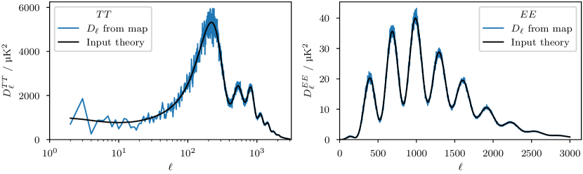
Figure 1: Comparison of taking a pure smooth theoretical CMB power spectrum, going to a map, and then computing the power spectrum once more. Note how the scatter increases for the lower multipoles and decreases at higher multipoles. This demonstrates the notion of “cosmic variance”, which is to say that we can only measure one sky, so the intrinsic variance on the lowest multipoles is large, since it can only be sampled a small number of times across the sky. A $TT$ example is shown on the left and $EE$ on the right.

6 The beam

When a CMB telescope points itself at the sky, it takes a fuzzy picture. We go from what is an infinite-resolution majesty down to a set of blurry blobs. This is the effect of the beam of the telescope, which averages the sky within its resolution element, with a shape that might be approximately Gaussian in the simplest case. This Gaussian will have some full-width-at-half-maximum (FWHM) size, often quoted as the telescope’s angular resolution. Real data processing can be much more complicated, with surveys like Planck having different beams for the different frequencies or even the different detectors, and with complicated scanning patterns. However, at its most basic level, the telescope’s optics consisted of a 2D Gaussian profile convolving our real sky. To emulate this when you are building a smoothed map, you should convolve the power spectrum with a Gaussian beam; HEALPix and healpy allow you to do this quite easily, with several Gaussian smoothing options, and options to smooth with a custom beam as well.

In the power spectrum the effect is to damp the power at the high $\ell$s; the smaller your beam the higher $\ell$ you retain good information on, and the bigger the beam the quicker you lose this information (see figs. 2 and 3).

To compute the spectrum profile $B_{\ell}$ of a Gaussian beam with standard deviation $\sigma$:

$$\mathrm{FWHM} =\sqrt{8\ln(2)}\sigma;$$ (11)

$$B_{\ell} =e^{-\frac{1}{2}\ell(\ell+1)\sigma^{2}};$$ (12)

$${}_{2}B_{\ell} =e^{-\frac{1}{2}\ell(\ell+1)\sigma^{2}}e^{2\sigma^{2}};$$ (13)

$$C_{\ell}^{\mathrm{obs}} =B_{\ell}^{2}C_{\ell}.$$ (14)

The factor of $e^{2\sigma^{2}}$ in eq. 13 is an approximation to go from the temperature or scalar field beam to the beam appropriate for the polarisation (or spin-2) fields (Challinor et al., 2000). This factor is typically small, e.g. for a beam with a FWHM of $5\text{\,}\mathrm{arcmin}$ it is $1+7.63\times 10^{-7}$. To simulate a real experiment, or to compare a real experiment to theory, it is important to include the beam in your considerations (either deconvolving the data with the beam or convolving the beam with your theory).

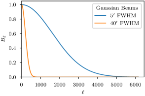
Figure 2: Comparison of beams of $5\text{\,}\mathrm{arcmin}$ and $40\text{\,}\mathrm{arcmin}$. The larger the FWHM the more quickly the higher modes are smoothed or damped out.

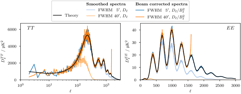
Figure 3: Comparison of power spectrum results from Gaussian-beam-smoothed maps for $TT$ and $EE$ power spectra. Dividing by the beam squared, in this case, returns a good approximation for the input theory. In more realistic cases, with noise for example, this division by the beam amplifies the noise at high $\ell$. It can also amplify numerical uncertainties at high $\ell$ when smoothing is more extreme, as seen in the spike around $\ell$ of 1500 in the deconvolved $\mathrm{FWHM}=$40\text{\,}\mathrm{arcmin}$$ case.

7 The pixel-window function

The pixel-window function is an often misunderstood step in the simulation process. What this does not do is model the pixelisation process performed by HEALpix. What it does do is model how observations on the sky are averaged into pixels. In a typical experiment, there will be many observations at many points on the sky and you will average these observations down into a single pixel. The pixel size is often chosen to have about 3 pixels per beam FWHM,. In any case, you must convolve with the pixel-window function to model this averaging step. Depending on the interest in higher multipoles, the size of the beam, and the pixelisation chosen, this will usually be less significant than the beam (but is still important!). Like the beam, this function can be arbitrarily complicated – since the telescope’s scanning pattern, the shape of the pixels, and the telescope’s beam may all come into play in the final averaging step. Nevertheless, it is often sufficient to use the pixel-window function provided by HEALPix and healpy to model this step (although it assumes that your beam is constant across the sky, the scanning pattern is uniform, and that the pixels are well and evenly sampled). You can see that the pixel window function is approximately a $\mathrm{sinc}$ function in the top panel of fig. 4:

$$P_{\ell}^{\mathrm{sinc}}=\mathrm{sinc}\left(\frac{\ell\theta_{\mathrm{r}}}{2\pi}\right)\,,$$ (15)

where $\theta_{\mathrm{r}}$ is the side length resolution of a pixel defined in eq. 1. The functions provided by HEALPix are more sophisticated, however, and should be used preferentially over the $\mathrm{sinc}$ approximation. The HEALPix window functions come from the actual spherical harmonic transform of an average HEALPix pixel for $N_{\mathrm{side}}$ less than 128, and extrapolated to higher $N_{\mathrm{side}}$ using a tophat approximation for the pixel (see Ref. Gorski et al. (1999)).

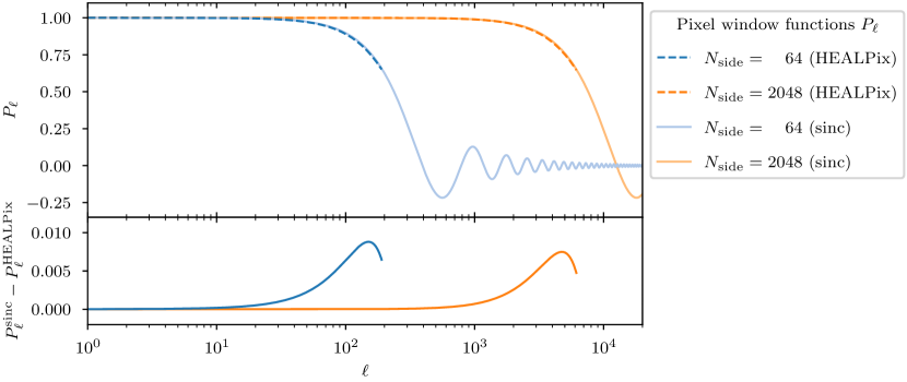
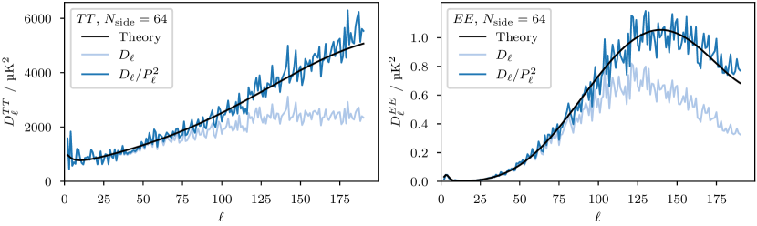
Figure 4: Effects of the pixel-window function. The top panel shows this function for different $N_{\mathrm{side}}$ values; the $N_{\mathrm{side}}=64$ map loses a significant amount of power by $\ell=150$, whereas for $N_{\mathrm{side}}=2048$ a similar amount of power is lost only by $\ell=5000$. The bottom panels show the resulting power spectra from a map convolved with the pixel window function at $N_{\mathrm{side}}=64$ and the deconvolved spectrum once divided by the pixel window function squared.

The beam and pixel-window functions are very similar in that each is an observation-driven effect, which reduces the observing power of a particular telescope at small scales (high-$\ell$ modes). Unlike the beam (which is driven entirely by the telescope’s specifications) the pixel window function has more flexibility. We focus on HEALPix for this paper, but many studies will choose to use Cartesian mapping and square pixels. What is important is that both the beam and the pixel-window function are well understood and accounted for in your analysis. Putting together the beam and the pixel effect, thus improving our model for a realistic sky, we now have

$$C_{\ell}^{\mathrm{obs}}=P_{\ell}^{2}B_{\ell}^{2}C_{\ell}\,.$$ (16)

8 Downgrading a map

It is common to downgrade the resolution of a CMB map; lower-resolution maps will have less noise per pixel, require fewer computing resources, and can be simpler to analyze. The cost is the loss of the higher resolution information (although this may be noise-dominated anyway). While it may be tempting to use the healpy or HEALPix function ud_grade, this will convolve your standard scalar CMB map (such as temperature, $E$ or $B$ maps) with the new pixel window function. It is, in essence, averaging all the information from the smaller pixels into the larger pixels and gives the appearance, mathematically, of convolving itself with the new pixel window function. This is an imperfect way to envisage this procedure, since the initial pixels may not very densely cover the final pixels, and if the initial map already had a beam or pixel window function applied to it then the final window function would need to account for all of those issues as well. This is perhaps argument enough that the ud_grade function should not be used to downgrade a typical CMB map. For the non-scalar maps, such as the $Q$ and $U$ polarisation maps, the ud_grade function should never be used, since it fails to correctly average the vectors in the $Q$ and $U$ maps, treating them as scalar values. Instead of using ud_grade when downgrading a map, one should first obtain the $a_{\ell m}$s of the map, and downgrade these in harmonic space. The functions used for HEALPix and healpy require that the highest $\ell$s of the input power spectrum are zero – for this reason, you must manually set these high $\ell$s to zero or risk there being excess power at small scales in your maps. Typically you want retain $\ell$ no higher than $\ell_{\mathrm{max}}=3N_{\mathrm{side}}-1$, or conservatively $\ell_{\mathrm{max}}=2N_{\mathrm{side}}$.

In fig. 5 we show the results from a simple map with no beam and no pixel window function downgraded from $N_{\mathrm{side}}=2048$ to $N_{\mathrm{side}}=64$. First, we downgrade using the ud_grade function, which results in low power at the highest $\ell$s due to the implicit convolution with the new pixel window function. This convolution cannot be fixed by simply deconvolving by the pixel-window function, since the initial map does not have very good coverage of the final pixels. Next, we take the same initial map and go to $a_{\ell m}$ space. From here we show the results of returning directly back to a lower resolution map, without nulling the high multipoles, and find that it leads to a large excess of power at the highest $\ell$s, in particular, this can be a substantial effect for the $EE$ power-spectrum. Lastly, we show the results after nulling $\ell$ modes above $3\,N_{\mathrm{side}}-1$ and above $2\,N_{\mathrm{side}}$ before returning to the lower resolution map. Both of these shows very good recovery of the input theory and map power spectrum.

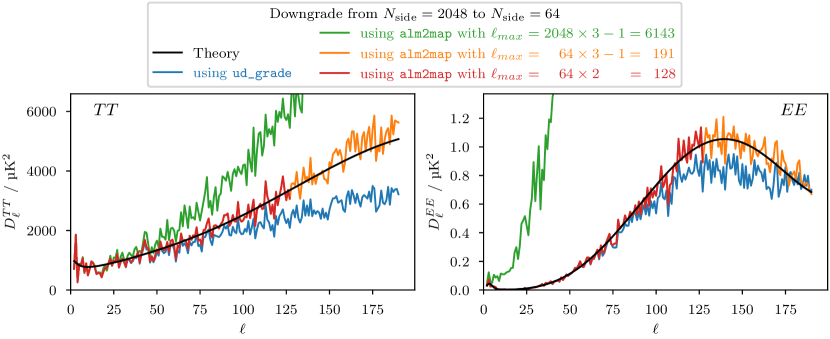
Figure 5: Results for different downgrading methods going from $N_{\mathrm{side}}=2048$ to $N_{\mathrm{side}}=64$. The correct downgrading method first takes the map to harmonic space ($a_{\ell m}$), zeros the high-$\ell$ components (above $3\,N_{\mathrm{side}}-1$, or conservatively above $2\,N_{\mathrm{side}}$) and finally converts to a map at a lower $N_{\mathrm{side}}$. In these panels, the orange and red lines show these scenarios. Using the healpy.ud_grade() function results in low power on small scales for the final maps, represented by the blue line. This averaging of the pixels has in effect convolved the map with some approximation of the new resolution’s pixel window function. The green line shows the results after failing to null the high $\ell$s, which leads to an overestimate of the power on the small scales – this can be quite extreme for the $E$ modes especially.

In realistic simulations your original map will have both a beam and a pixel window function; in this case, you must deconvolve with the original functions and reconvolve with the new pixel window function and beam:

$$a_{\ell m}^{\mathrm{new}}=\left.\frac{B_{\ell}^{\mathrm{new}}P_{\ell}^{\mathrm{new}}}{B_{\ell}^{\mathrm{old}}P_{\ell}^{\mathrm{old}}}a_{\ell m}^{\mathrm{old}}\right\rvert_{0}^{\ell_{\mathrm{max}}},$$ (17)

where $\ell_{\mathrm{max}}$ is the new maximum multipole for the lower $N_{\mathrm{side}}$. In the case where there are foreground contaminants that you plan to mask later in the analysis, it is a good idea to downgrade the mask similarly. The new mask can be reconverted to binary by choosing a threshold (typically 0.9) to reset the values lower than the threshold to zero, and higher to one. You can choose the threshold to ensure that any foreground contaminants that leak beyond the range of the original mask are still masked in the new downgraded mask. You should downgrade the map before masking as well, if at all possible, to ensure that no masking effects are introduced through this process.

9 White noise

The simplest noise properties to add to the data is white noise, which is flat in $C_{\ell}$ space. Additional complexities including the scanning pattern of the telescope, $1/f$ noise, foreground residuals and other details can be added with additional effort, but for the simplest case (as is often desired when troubleshooting code for example), white noise is a good starting point. Adding white noise is a simple procedure and may be done at the map level or the power spectrum level. White noise is a constant addition to each of the multipoles in the power spectrum (in effect simply increasing the standard deviation for each of the modes), or a random number with a mean of zero and a standard deviation at the level of the noise added to each of the pixels in a map. Given the noise $\epsilon$ in units of [inter-unit-product=${}\cdot{}$]′, the noise per multipole is the conversion from arcminutes to radians squared,

$$\epsilon_{\ell}=\epsilon^{2}\left(\frac{\pi}{60\times 180}\right)^{2},\qquad\text{with }[\epsilon_{\ell}] =\unit{\squared}$$

$$[\epsilon] =\unit[inter-unit-product={}\cdot{}]{\arcmin},$$ (18)

and the noise per pixel $\epsilon_{\mathrm{pix}}$ is the division by the side length resolution $\theta_{\mathrm{r}}$ in arcminutes,

$$\epsilon_{\mathrm{pix}}=\frac{\epsilon}{\theta_{\mathrm{r}}},\qquad\text{with }[\epsilon_{\mathrm{pix}}] =\unit{},$$ (19)

$$[\epsilon] =\unit[inter-unit-product={}\cdot{}]{\arcmin},$$ (20)

$$[\theta_{\mathrm{r}}] =\unit{\arcmin}.$$ (21)

As expected, the noise is lower for larger pixels and larger for smaller pixels and is flat in $\ell$ space. As an example, the noise in the Planck maps was around $2.3\text{\times}{10}^{-5}\text{\,}\mathrm{K}\text{\,}\mathrm{arcmin}$, so the noise per pixel in an $\epsilon_{\mathrm{side}}=2048$ map would be around $1.3\text{\times}{10}^{-5}\text{\,}\mathrm{K}$, since a pixel has a resolution of $1.72\text{\,}\mathrm{arcmin}$, and $\epsilon_{\ell}$ would be $4.5\text{\times}{10}^{-5}\text{\,}{\mathrm{\SIUnitSymbolMicro K}}^{2}$. Often the noise in the temperature maps will be a factor of $\sqrt{2}$ smaller than that in the $Q$ and $U$ maps, due to the way the data are split, with full data included in the temperature maps, and half the data included in each of the polarisation maps.

Depending on how your noise is defined, it generally should not be convolved with the beam and the pixel window function, since this would artificially damp the high-$\ell$ noise (for pure flat white noise). So we now have

$$C_{\ell}^{\mathrm{obs}}=P_{\ell}^{2}B_{\ell}^{2}C_{\ell}+\epsilon_{\ell}\,,$$ (22)

which accounts for the beam and pixel window functions applied to the sky, as well as the white noise. The noise will be a much smaller portion of the temperature power spectrum than for the $E$-mode power spectrum (see fig. 6).

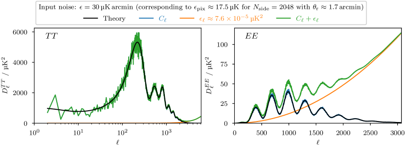
Figure 6: The effect of adding white noise added to the power spectrum. In this idealistic case, there is no beam or pixel window function and the noise has been added directly to the power spectrum, not the map. The noise level applied here was $\epsilon_{\ell}=$7.6\text{\times}{10}^{-5}\text{\,}{\mathrm{\SIUnitSymbolMicro K}}^{2}$$ or $\epsilon=$30\text{\,}\mathrm{\SIUnitSymbolMicro}\mathrm{K}\cdot\mathrm{arcmin}$$. In a more realistic scenario the noise levels for temperature and polarisation would be different, but for simplicity we are assuming the same noise here. Note that since we plot $D_{\ell}$, the otherwise constant noise spectrum $\epsilon_{\ell}$ increases with $\ell^{2}$.

10 The mask

Of the procedures described in these notes, masking is likely the most complicated topic that will be discussed. Put simply, the mask should null out areas of the sky that are heavily contaminated with residuals. For the CMB, this is usually the region along the Galactic plane where foregrounds are dominant, but could also involve masking areas of point sources outside the Galactic plane.

The simplest mask will consist of ones and zeros, but the sharp edges of the mask can lead to ringing in the final power spectrum, since you are effectively applying a 2D top hat filter to a sky, and then taking the spherical equivalent of a Fourier transform. One way to reduce the ringing is to soften the mask edges through ‘apodisation’. How you choose to apodise, and by how much, should be carefully considered and tested on any analysis you might perform. Additionally, the method you use to go from the map to the power spectrum and back should be done with care. For high $\ell$ it is preferable to use a pseudo-$C_{\ell}$ approach, such as the MASTER (Hivon et al., 2002) method used by codes like NaMaster (Alonso et al., 2023), while for the low $\ell$ it is better to use a quasi-maximum likelihood (QML) method, such as in Eclipse (Bilbao-Ahedo et al., 2021, 2023) and xQML (Vanneste et al., 2018). There are also methods such as PolSpice (Challinor et al., 2011) that use the correlation estimator in map space to estimate the power spectrum. I will not recommend the use of any one particular mask, apodisation technique or spherical harmonic decomposition technique, but rather aim to emphasize the complexities associated with masking.

To emphasize the effect of apodisation (of which pymaster, the Python wrapper of NaMaster, provides a few options), I analyse the impact of the mask on the power spectrum estimate for a range of map types. Specifically, I use the so-called “common” Planck mask, a pure Galactic-cut mask, along with a point source mask. All the masks are provided on the PLA in their un-apodised form and for $N_{\mathrm{side}}=2048$.

I have used the ‘C1’ apodisation provided by NaMaster on all of them with an apodisation length of $0.5\mathrm{°}$ and $5.0\mathrm{°}$, which smoothly interpolates over that length scale between the zero and one values of the binary masks. Figure 7 gives an overview of all these masks, and fig. 8 shows how apodisation improves the power spectrum estimation, greatly expanding the well recovered multipole range.

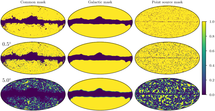
Figure 7: Masks compared in this analysis, top to bottom increasing in apodisation length, and left to right the “common” mask (for intensity, there is another common mask specifically for polarisation), the $20\text{\,}\mathrm{\char 37\relax}$ Galactic mask (leaving $80\text{\,}\mathrm{\char 37\relax}$ of the sky unmasked), and the point-source mask (for the Planck lower frequency channels). Yellow corresponds to unmasked regions whereas dark purple and gradient colours between are masked and apodised regions, respectively.

Depending on the technique used to estimate the $C_{\ell}$s, the mask will reduce the amplitude of the power spectrum, which can be corrected by multiplying the theory (or dividing the observation) by the fraction of the sky masked;

$$f_{\mathrm{sky}}=\frac{1}{N_{\mathrm{pix}}}\sum_{i=0}^{N_{\mathrm{pix}}}M_{i}^{2},$$ (23)

where $M_{i}=0$ if masked and $M_{i}=1$ if unmasked for the un-apodised mask, otherwise $M_{i}$ will be some value ranging from 0 to 1 for unmasked pixels. The effect of this $f_{\mathrm{sky}}$ correction is illustrated in fig. 8, where the light grey line corresponds to the healpy $C_{\ell}$ estimate before correction, and the dark grey line to the estimate after correction. Adding in the masking $f_{\mathrm{sky}}$ correction, we finally have

$$C_{\ell}^{\mathrm{obs}}=f_{\mathrm{sky}}\left(P_{\ell}^{2}B_{\ell}^{2}C_{\ell}+\epsilon_{\ell}\right)\,,$$ (24)

such that we have accounted for the beam, pixel window function, noise, and power reduction due to the mask.

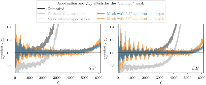
Figure 8: Mask apodisation effects. Applying a mask to a CMB map can lead to complicated coupling effects so obtaining the correct power spectrum from the map must be done with care. Here I show the estimated power $C_{\ell}^{\mathrm{masked}}$ from maps masked with the Planck “common” mask relative to the power spectrum $C_{\ell}$ from the unmasked map. The left panel shows the results for the temperature spectrum and the right panel the results for $E$-mode polarisation. Dividing the observed power by the unmasked sky fraction $f_{\mathrm{sky}}$ is an important step in correctly estimating the overall power, but this does not solve the issue that at small scales (high $\ell$) the power tends to be overestimated. Apodising a mask greatly extends the correctly estimated multipole range. However, too extreme an apodisation can eventually degrade the estimate again.

Apodisation and $f_{\mathrm{sky}}$ correction might not be enough, though. Some mask types come with unique challenges, e.g. the point source mask introduces heavy ringing in healpy’s power spectrum estimate, as demonstrated in fig. 9. This ringing effect can be mitigated by switching to pymaster (see fig. 10), but it comes at the cost of overall larger uncertainty of the estimate.

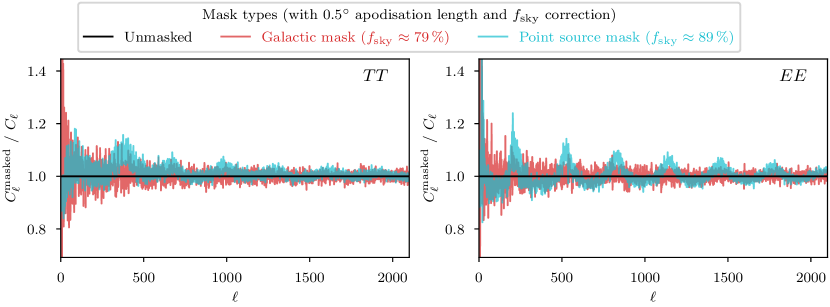
Figure 9: Same plot as in fig. 8, but now highlighting the effect of different mask types, specifically the difference between a Galactic mask in the form of a smooth belt around the equator and a point source mask in the form of many disconnected circular spots (see fig. 7 for a visual comparison). Both masks were apodised before power estimation, and both resulting $C_{\ell}^{\mathrm{masked}}$ estimates were corrected with the corresponding sky fraction. Overall the power estimates are close to the expected values, but there is a clear ringing effect in the results with the point source mask.

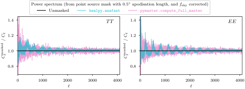
Figure 10: Same plot as in fig. 8, but now highlighting two different power spectrum estimation functions, one from healpy and the other from pymaster. The latter manages to recover the unmasked $C_{\ell}$ slightly better, and visibly reduces the ringing effect from the point source mask.

11 Final steps and summary

Let me summarise by listing the steps for generating a simple CMB map realisation with white noise.

1. Generate from CAMB or CLASS the desired power-spectrum $C_{\ell}$ (or download a pre-computed one, e.g. from the PLA).

2. Convolve the power spectrum with the beam $B_{\ell}$ and pixel window function $P_{\ell}$.

3. Add the desired noise spectrum $\epsilon_{\ell}$.

4. Generate the map (from the randomised $a_{\ell m}$s).

5. Mask the map (ensure that the mask is apodised for certain procedures).

From the map (before masking), there are a few possible procedures, such as downgrading the map resolution, which I now list.

1. Starting from the input map, obtain the $a_{\ell m}$ from the map and the mask.

2. Cut all the $\ell$s above $2$$N_{\mathrm{side}}$ (conservatively), or 3$N_{\mathrm{side}}$$-1$ (less conservatively).

3. Deconvolve by the beam and the pixel window function and reconvolve by the new beam and the new pixel window function.

4. Downgrade the mask in the same way as the map. The new mask will be extended to account for regions of the sky that were originally masked leaking into unmasked regions. Choose some threshold for this step and re-apodise the mask.

5. Generate the new map at the lower resolution, and apply the new downgraded mask.

Returning to the power spectrum, these are a few more steps.

1. From a masked map you should first remove the dipole and the monopole (these are generally masking effects and will alter the effectiveness of the final results).

2. Ensure the applied mask was apodised, or apply an apodised mask to the map.

3. Obtain the low-order $C_{\ell}$ using QML or anafast and the higher orders using a pseudo-$C_{\ell}$ method such as NaMaster to control for the effects of the mask. If anafast is used throughout then you must divide by the sky fraction to obtain the correct amplitude of the underlying $C_{\ell}$s.

4. Divide the $C_{\ell}$s by the beam and pixel window functions squared. The noise will dominate at the high $\ell$ compared to the signal.

To summarize, going from a CMB map to a power spectrum and back should be done with care, but following the correct procedures will introduce relatively few artefacts, and allow for the effective analysis of the data in either map space or harmonic space. Any steps taken should be well understood and tested, and any results should be robust against choices made, such as resolution, beams, masks used, and the methods used to go from the map to harmonic space and back again.

References

- Alonso et al. (2023) Alonso, D., Sanchez, J., Slosar, A., & LSST Dark Energy Science Collaboration. 2023, Astrophysics Source Code Library
- Bilbao-Ahedo et al. (2021) Bilbao-Ahedo, J. D., Barreiro, R. B., Vielva, P., Martínez-González, E., & Herranz, D. 2021, JCAP, 2021, 034, doi: 10.1088/1475-7516/2021/07/034
- Bilbao-Ahedo et al. (2023) —. 2023, Astrophysics Source Code Library
- Blas et al. (2011) Blas, D., Lesgourgues, J., & Tram, T. 2011, Journal of Cosmology and Astroparticle Physics, 2011, 034, doi: 10.1088/1475-7516/2011/07/034
- Challinor et al. (2011) Challinor, A., Chon, G., Colombi, S., et al. 2011, Astrophysics Source Code Library
- Challinor et al. (2000) Challinor, A., Fosalba, P., Mortlock, D., et al. 2000, Phys. Rev. D, 62, 123002, doi: 10.1103/PhysRevD.62.123002
- Górski et al. (2005) Górski, K. M., Hivon, E., Banday, A. J., et al. 2005, ApJ, 622, 759, doi: 10.1086/427976
- Gorski et al. (1999) Gorski, K. M., Wandelt, B. D., Hansen, F. K., Hivon, E., & Banday, A. J. 1999, arXiv e-prints, astro, doi: 10.48550/arXiv.astro-ph/9905275
- Grain et al. (2009) Grain, J., Tristram, M., & Stompor, R. 2009, Physical Review D, 79, 123515, doi: 10.1103/PhysRevD.79.123515
- Hivon et al. (2002) Hivon, E., Górski, K. M., Netterfield, C. B., et al. 2002, ApJ, 567, 2, doi: 10.1086/338126
- Hu & White (1997) Hu, W., & White, M. 1997, New A, 2, 323, doi: 10.1016/S1384-1076(97)00022-5
- Kamionkowski et al. (1997) Kamionkowski, M., Kosowsky, A., & Stebbins, A. 1997, Phys. Rev. D, 55, 7368, doi: 10.1103/PhysRevD.55.7368
- Kamionkowski & Loeb (1997) Kamionkowski, M., & Loeb, A. 1997, Phys. Rev. D, 56, 4511, doi: 10.1103/PhysRevD.56.4511
- Lesgourgues (2011a) Lesgourgues, J. 2011a, The Cosmic Linear Anisotropy Solving System (CLASS) I: Overview. https://arxiv.org/abs/1104.2932
- Lesgourgues (2011b) —. 2011b. https://arxiv.org/abs/1104.2934
- Lesgourgues & Tram (2011) Lesgourgues, J., & Tram, T. 2011, Journal of Cosmology and Astroparticle Physics, 2011, 032, doi: 10.1088/1475-7516/2011/09/032
- Lewis & Challinor (2011) Lewis, A., & Challinor, A. 2011, Astrophysics Source Code Library
- Lewis et al. (2000) Lewis, A., Challinor, A., & Lasenby, A. 2000, ApJ, 538, 473, doi: 10.1086/309179
- Mortlock et al. (2002) Mortlock, D. J., Challinor, A. D., & Hobson, M. P. 2002, MNRAS, 330, 405, doi: 10.1046/j.1365-8711.2002.05085.x
- Reinecke & Seljebotn (2013) Reinecke, M., & Seljebotn, D. S. 2013, A&A, 554, A112, doi: 10.1051/0004-6361/201321494
- Scott et al. (1994) Scott, D., Srednicki, M., & White, M. 1994, ApJ, 421, L5, doi: 10.1086/187173
- Tegmark (1997) Tegmark, M. 1997, Phys. Rev. D, 56, 4514, doi: 10.1103/PhysRevD.56.4514
- Vanneste et al. (2018) Vanneste, S., Henrot-Versillé, S., Louis, T., & Tristram, M. 2018, Phys. Rev. D, 98, 103526, doi: 10.1103/PhysRevD.98.103526
- Zonca et al. (2019) Zonca, A., Singer, L., Lenz, D., et al. 2019, Journal of Open Source Software, 4, 1298, doi: 10.21105/joss.01298