SoK: On Finding Common Ground in Loss Landscapes Using Deep Model Merging Techniques

Abstract

Understanding neural networks is crucial to creating reliable and trustworthy deep learning models. Most contemporary research in interpretability analyzes just one model at a time via causal intervention or activation analysis. Yet despite successes, these methods leave significant gaps in our understanding of the training behaviors of neural networks, how their inner representations emerge, and how we can predictably associate model components with task-specific behaviors. Seeking new insights from work in related fields, here we survey literature in the field of model merging, a field that aims to combine the abilities of various neural networks by merging their parameters and identifying task-specific model components in the process. We analyze the model merging literature through the lens of loss landscape geometry, an approach that enables us to connect observations from empirical studies on interpretability, security, model merging, and loss landscape analysis to phenomena that govern neural network training and the emergence of their inner representations. To systematize knowledge in this area, we present a novel taxonomy of model merging techniques organized by their core algorithmic principles. Additionally, we distill repeated empirical observations from the literature in these fields into characterizations of four major aspects of loss landscape geometry: mode convexity, determinism, directedness, and connectivity. We argue that by improving our understanding of the principles underlying model merging and loss landscape geometry, this work contributes to the goal of ensuring secure and trustworthy machine learning in practice.

I Introduction

Deep learning is now ubiquitous in various domains, from natural language processing [1] and computer vision [2] to time-series forecasting [3]. However, the sheer size and complexity of modern neural networks make it difficult to interpret the features they learn. This opacity poses issues for adoption in safety-critical applications such as healthcare [4], autonomous vehicles [5], and nuclear energy [6], where decision-making failures can be catastrophic. Moreover, deep learning practitioners, aware of the risks of harm associated with deploying neural networks, desire strategies to mitigate their potential misuse. Deep learning models are known to hallucinate faulty information [7], aid in creating inappropriate content [8], leak sensitive training data [9, 10, 11], and learn biased decision boundaries [12, 13]. Without a proper understanding of the inner mechanisms of neural networks, and specifically how neural network components relate to behaviors, we cannot develop effective solutions for the safe and ethical deployment of neural networks.

A subfield of deep-learning that extensively studies procedures for associating neural network components (e.g., layers, neurons, or weights) with specific behaviors is model merging. Model merging explores procedures for altering the weights of existing models to produce more performant and generalizable predictors. A common motivation is to reuse existing models, especially as the time, computing infrastructure, and energy required to train models grow. The model merging problem is presented as follows: Given the parameters of several sources models $\theta_{1},\theta_{2},\ldots,\theta_{n}$, we seek to develop a merging procedure $f(\theta_{1},\theta_{2},\ldots,\theta_{n}):\Theta^{n}\mapsto\Theta$ to produce a new merged model $\theta^{\star}$ that minimizes some loss $\mathcal{L}(\theta)$. In particular, the merging methods produce a single model from several previously trained models, in contrast to traditional ensemble methods (see Section IV)—precursors for model merging techniques—that require several models for inference incurring high latency costs. Thus, model merging can act as a cheaper alternative to ensembling. However, ensemble techniques need only combine models’ prediction logits, whereas model merging techniques must compress several networks into a single model, leading to more potential points of failure. Empirical evidence suggests that neural networks form highly compressed representations of their training data—even more so as they are overparameterized—resulting in sparse networks that can be pruned to a fraction of their original size [14, 15]. In principle, we should be able to exploit this sparsity to effectively merge neural networks trained on different tasks, but in practice, merging models trained on different tasks is challenging [16, 17, 18]. By contrast, ensemble methods are consistently successful in this endeavor. Moreover, simply training a monolithic multi-task model often outperforms both ensembling and merging—forming a practical upper bound in performance for both techniques.

Model merging is complicated by the permutation-invariant nature of neural networks (see Section III-B2), which prevents straightforward averaging between corresponding parameter values in each layer due to potential misalignment between layers of neurons without degrading performance [16, 19, 20]. Additionally, merging methods tend to degrade in performance as the training distributions of source models diverge from one another [19, 20, 21, 22]. This degradation is an issue in real-world scenarios—such as financial forecasting, meteorology, facial recognition, and medical prognosis tasks [23, 24]—that experience distributional shift over time. Merging methods also scale in cost with the number of parameters in each source model, making application to large models expensive. Some procedures also require further computation to produce additional artifacts—such as approximations to the Fisher matrix [25, 26]—that aid in weighting and aligning the parameters of source models. Moreover, in decentralized scenarios, such as federated learning [27], merging incurs communication costs proportional to model size and any intermediate artifacts used for merging, which may become a bottleneck for continuous training and merging procedures.

I-A Relevance to Safe and Trustworthy Machine Learning

Model merging techniques provide procedures for associating individual weights, neurons, or layers with specific behaviors. These procedures are analogous to circuit-discovery algorithms in interpretability that seek to isolate behaviors to particular neurons or layers by analyzing activations—for example, by identifying topic-specific attention heads in large language models (LLMs) [28]. Model merging algorithms also alter model behavior and knowledge by manipulating model parameters. These algorithms can be considered a parameter space analog to popular interpretability techniques, such as activation steering, which seek to bias model behavior in a particular direction by altering model activations [29]. Similarly, model merging techniques are relevant to efforts in machine unlearning and have already been applied successfully to reduce memorization in LLMs [30].

Many deep learning applications must defend against adversaries—malicious actors seeking to extract sensitive data, degrade model performance, or abuse models for inappropriate use cases. For example, in healthcare, the consequences of poor model performance in diagnostic and prognostic tasks can be life-threatening—these models must be robust to adversaries [31]. Healthcare providers may seek to accelerate medical research by using decentralized machine learning techniques, such as Federated Learning [32], to create robust models without directly sharing patient data between facilities [33]. Unfortunately, decentralized model updates may risk unintentionally leaking private data by sending parameters or gradient updates across a network [34] and allowing the introduction of adversarial examples that degrade overall model performance [33, 35, 36, 37]. The model merging literature can help explain the susceptibility of models to training data extraction attacks [9]. Additionally, many model merging techniques, such as RegMean (see Section V-C), present techniques to perform decentralized model merging without leaking data samples. Moreover, the literature on model merging sheds insight into how adversarial examples might be thwarted and how we can manipulate model parameters to obtain more robust, performant deep learning solutions [38, 39, 40].

I-B Contributions

In this work, we explore model merging techniques through the lens of loss landscape geometry (see Section III-B) to illuminate potential areas of interest for interpretability and security researchers. We make the following contributions:

1. We propose a taxonomy of model merging techniques focused on enumerating their core algorithmic principles.

2. We synthesize empirical data from many model merging studies to characterize phenomena that manifest on objective landscapes during training.

3. We draw meaningful connections between model merging and research in model interpretability and security.

This paper is organized as follows: Section III defines some relevant terminology and introduces prerequisite concepts from the study of loss landscapes; Sections IV, V, and VI survey model merging research covering ensemble, weight aggregation, and neuron alignment techniques for model merging, respectively; Section VII synthesizes the empirical observations from this survey into descriptions of loss landscape geometry to characterize commonly observed phenomena during model training; Section VIII discusses the implications of our analysis on model interpretability and security; and Section IX proposes directions for future investigation in light of our analysis.

II Related Surveys

While the model merging literature is extensive, we know of only a handful of other surveys in this area [41, 42, 43, 44]. Li et al. [41] and Yadav et al. [42] focus their discussion of model merging on two particular application areas, namely federated learning and mixture-of-experts regimes, and include techniques that do not attempt to manipulate weights directly, such as knowledge distillation. Meanwhile, Yang et al. [44] survey a range of merging techniques and taxonomize techniques according to when they are applied during the training pipeline, focusing on their relevance to application domains such as alignment, continual learning, and multimodal fusion. Li et al. [43] present a survey with a taxonomy similar to ours but focus on their application to federated learning, knowledge distillation, and fine-tuning.

By contrast, our work presents a taxonomy of model combination techniques organized into just three major categories: ensembling, weight aggregation, and neuron alignment (see Fig. 1). We do not include techniques that require full training runs, such as knowledge distillation. Our work focuses explicitly on extracting insights into how training proceeds under SGD, connecting the success of model merging techniques to the underlying structure of the loss landscape, and applying these ideas to model interpretability and security.

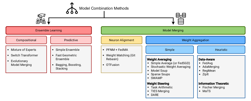
Figure 1: A taxonomy of model combination methods. Ensemble methods do not manipulate model parameters, but rather combine prediction logits or model components in novel ways. Neuron Alignment techniques attempt to resolve potential misalignment between model representations by using permutations of their units before computing some linear combination of source model parameters. Weight Aggregation methods compute a linear combination of model parameters.

III Background

Model merging is intimately connected to the study of loss landscapes and their geometry. Here, we introduce concepts from the loss landscape literature that inform contemporary approaches to model merging.

III-A Model Spaces

Deep learning literature deals with several “spaces” over which we can analyze models. For clarity, we define these spaces here. Parameter space or weight space refers to the space of all model parameters. This is generally the domain of model merging techniques, which seek to analyze the weights of models and alter behavior via interventions on weights. Activation space refers to the space of all model activations. That is, the set of possible activation values at each layer in a particular deep learning model. This is generally the domain of interpretability techniques that compute summary statistics describing the relationship between data and model activations to isolate model components of interest.

III-B Loss Landscapes

The loss landscape (also referred to as the objective landscape) of a deep learning architecture is the high-dimensional surface induced by the loss function when evaluated over the domain of all possible parameter values [45]. Loss landscape geometry refers to the geometric structure of the loss landscape, including the location of local minima and their relation to one another. A key concept is the idea of an objective mode—a particular local minimum of the loss landscape. An objective mode lies in an objective basin (or loss basin), which is comprised of the objective mode and the surrounding locally convex region of solutions. Model merging methods must account for the structure of the loss landscape to synthesize performant solutions from existing models. Therefore, studying model training behavior and loss landscape geometry is crucial to developing effective model merging techniques. Below, we review fundamental loss landscape concepts.

III-B1 Mode Connectivity

Consider a given path, $p(\theta_{a},\theta_{b},\lambda)$, between two models $\theta_{a}$ and $\theta_{b}$ parameterized by $\lambda\in[0,1]$. We will refer to $\theta_{a}$ and $\theta_{b}$ as the endpoints of the path. The loss barrier, defined below in Eq. (missing) 1, on the path $p$ is defined as the maximum increase in loss along $p$ over the average loss of both endpoints.

$$\mathcal{L}_{p}=\max_{\lambda\in[0,1]}\mathcal{L}(p(\theta_{a},\theta_{b},\lambda))-\frac{1}{2}(\mathcal{L}(\theta_{a})+\mathcal{L}(\theta_{b}))$$ (1)

Two models are said to exhibit Mode Connectivity if there exists a path $p$ between them where the loss barrier is approximately zero [46, 47, 19]. Linear Mode Connectivity (LMC) [48, 47] is a stronger condition asserting that two modes can be connected by a straight line—of special interest as linearly connected solutions may lie in the same convex basin. Mode-connecting paths reveal the structure of the loss landscape and allow us to find diverse but equally performant solutions between two known models [49].

In practice, we can discover paths of low loss between distinct neural networks via optimization (e.g., by parameterizing a Bézier curve) [50, 51, 46, 52, 53]. Surprisingly, solutions are often connected by simple curves, and even linear mode connectivity seems commonplace [50, 47]. Recent work has exploited this fact to ensemble networks that are close in the objective landscape, indicating that despite lying close together, sufficient diversity exists between these solutions to provide an advantage from ensembling [50]. Some empirical evidence suggests that geodesics between neural networks in the distribution space induced by the Fisher-Rao metric may correspond to paths between their parameters in objective space [52]. This finding links the notions of mode connectivity and interpolating between distributions. Additionally, it has been shown that linear interpolation between the parameters of two linearly connected models corresponds to linear interpolation between their activation maps [39]. This property holds even when the endpoints of interpolation are two networks fine-tuned on distinct tasks, provided that they stem from the same pre-trained checkpoint (see Section III-B3) [54].

III-B2 Permutation Symmetry

Neural networks inherently have components that are invariant to permutations. For example, in a single linear layer of neurons, any permutation in the order of neurons would still result in the same activations for that layer. Therefore, we can consider any neural network to be a member of an equivalence class of other neural networks whose units are permuted but whose activations are the same. This permutation-invariance property has led some to conjecture that all solutions to Stochastic Gradient Descent (SGD) can be linearly connected if the natural permutation invariance of neural networks is accounted for [16]. This conjecture has spurred further investigation into the permutation symmetries inherent in the layers of neural networks and attempts to resolve them to achieve LMC between different solutions.

Several theoretical results demonstrate that the objective landscapes of over-parameterized models are dominated by permutation-equivalent objective modes and that valleys in the loss landscape can be connected through permutation points [55, 56]. Additionally, many merging works provide substantial empirical evidence that aligning neurons by learning appropriate permutations in their order reveals linearly connected paths between models (see Section VI) [19, 20, 57, 51, 58]. This property holds even when models are trained on slightly differing data distributions [19, 20]. It has been observed that models trained on similar underlying distributions tend to have a similar distribution of singular values but may differ in their corresponding singular directions. This observation has led some to propose that the success of neuron alignment methods can be explained by the resulting alignment of dominant singular directions in the weight matrices by learned permutations of the order of neurons [59]. This observation suggests we can meaningfully associate task-specific performance with just a few singular directions in parameter space [59, 60].

III-B3 Training Trajectories

The position of a neural network in the objective landscape is determined by the interaction between loss landscape geometry and gradient descent. Therefore, understanding training trajectories is paramount in model merging. A training trajectory is a sequence of points, each representing the parameters of a neural network, that evolves under some optimization algorithm, such as SGD, during the training process. Numerous efforts have been made to characterize how training proceeds from distinct initialization points under SGD and how this relates to the underlying objective landscape. Empirically, researchers have observed that SGD is initially unstable but soon reaches a “stable point”. After this point, subsequent fine-tuning causes networks to converge to the same loss basin even under different forms of SGD noise (e.g., batch order) [61, 47]. Some work has also demonstrated the converse, that deep neural networks with different random initializations learn functions with distinct properties and lie in distinct regions [62]. These works all support the conclusion that neural networks that share a significant portion of their training trajectory tend to lie in the same linearly connected region of the objective landscape. Conversely, those that are initialized separately lie in distinct regions of the objective landscape. A corollary of this finding is that models in the same objective basin generally do not require any form of neuron alignment for merging [21].

IV Ensembling

Ensembling is the most widely applied and reliable method to combine knowledge between models [63]. Ensemble methods are precursors to modern model merging techniques. In this section, we review the origins of ensembling and several prominent ensembling methods to frame our subsequent discussion of model merging techniques.

IV-A Overview

Ensembling combines the predictions (as opposed to parameters) from several trained models to enhance accuracy at inference-time. Ensembles compute a weighted combination of output predictions from each model in the ensemble to form a prediction. The success of ensemble methods is often attributed to a reduction in model bias and variance that occurs when predictions are averaged from several statistical models [62, 63]. Ensembling is closely related to Bayesian Model Averaging techniques [64]. In classic Bayesian Model Averaging, the final prediction is a weighted average of the predictions of each of our models, weighted by the posterior probability of each model [65].

For neural networks, the posterior probabilities are calculated over different weight settings:

$$p\left(y\mid x,D\right)=\int p\left(y\mid x,\theta\right)\;p\left(\theta\mid D\right)\,d\theta$$ (2)

where $y$ is the data label, $x$ the input data, $D$ the training data, and $\theta$ the neural network parameters. Integrating over all weight settings for a neural network is intractable; however, many works observe that neural networks consistently converge to solutions lying in large, flat basins in the loss landscape [64, 66, 67, 68, 69]. One explanation for this behavior is that these flat areas occupy large volumes in parameter space, and thus, stochastic gradient descent is exponentially more likely to land in these regions [66]. From a Bayesian perspective, these large, flat areas in parameter space have high probability density, $p\left(\theta\mid D\right)$, in the integral above. Therefore, an ensemble where we take the average predictions of several trained neural networks [70] can be thought of as an approximation of a Bayesian calculation of the posterior probability of $y$, with the integral estimated by the normalized summation of a few high probability parameter settings.

IV-B Ensemble Techniques

Despite the reliability of ensemble methods, they can be impractical because they require training and deploying several deep neural networks simultaneously. Some methods attempt to reduce the cost of obtaining several models to be used as ensemble members. Snapshot Ensembles cycle through learning rates during training to produce several diverse models at various minima within a single training run [71]. Another approach is to exploit the local loss geometry around an existing model to discover useful ensemble members; for example, sampling new models from within the same objective basin as an existing model—as done in Fast Geometric Ensembling (FGE) [50]. This idea exploits the linear connectivity within an objective basin but has since been extended to exploit more complex forms of Mode Connectivity in the loss landscape. Benton et al. [72] develop a method that finds whole simplices of low loss in the objective landscape that connect several potential solutions. This method closely approximates a classic Bayesian model average where the posterior is uniformly distributed over a simplex.

In addition to algorithmic advancements, recent increases in the number of freely available models have also reduced the cost of constructing ensembles. More pressing is the issue of runtime and memory efficiency, each of which scales linearly with the number of models in the ensemble. Mixture-of-Experts (MoE) routines reduce the inference cost associated with ensembling to that of a single model [73]. Rather than averaging the predictions of each ensemble member, these methods learn to compose components—at the granularity of whole networks, layers, or individual neurons—from each model to compute the final output prediction. This amounts to learning how to construct a new neural network for each input presented. Evolutionary Model Merging is a similar technique that uses an evolutionary algorithm to compose layers from each ensemble member to construct a new network [74].

IV-C Limitations of Ensembling

Ensembles of several models have become much more straightforward to obtain thanks to advancements in our understanding of the loss landscape [50, 72, 71]. Still, ensemble techniques suffer from poor scaling in terms of runtime and memory costs, as we must use multiple models for inference. MoE methods are a boon for use cases where inference cost is a limiting factor. Unfortunately, MoE methods are not necessarily a universal solution. While the effective parameter count for a given input in a MoE model is lower, the total number of parameters in the mixture may be the same or even greater [75]. As individual “experts” in the mixture specialize in just a few prediction domains, we must train more parameters in total to achieve strong performance across all domains. Consequently, training and serving MoE models requires constantly exchanging large numbers of parameters from memory. This requires a significant investment in complex infrastructure to serve models of billions or trillions of parameters. MoE models also exhibit decreased sample efficiency during training; each parameter is not trained during every batch, increasing training costs. Though these methods offer exciting avenues for scaling and deploying ensemble models more efficiently, model merging offers the potential for equivalent performance at a significant cost reduction.

Figure 2: Mode Convexity: Within an objective basin, one can linearly interpolate between known solutions to discover equally performant models with diverse behaviors.

V Weight Aggregation

The fundamental technique underlying most model merging methods is weight aggregation. Given two or more models of the same architecture, one can compute an average or sum over the values for each corresponding parameter to obtain a set of new parameter values that comprise the merged model. These techniques are predicated on the principles of Bayesian Model Averaging, seeking to reduce estimation error from individual model bias and variance by combining several models for inference [76]. Though weight aggregation methods show promise compared to ensemble methods, they also introduce several challenges. Weight aggregation methods usually introduce additional hyperparameters that must be set via trial-and-error or by some heuristic method. Additionally, their failure modes are not fully understood. While some characterizations of their failure cases can be extrapolated from the literature (see Section VI below), more context on loss landscape geometry is necessary to fully understand their modes of failure. Below, we discuss several modes of weight aggregation, including simple averaging, weight steering via task arithmetic, and heuristic weighted averaging.

V-A Simple Averaging

The most straightforward method of merging model parameters is to take a simple average over each corresponding parameter between two or more models, see Eq. (missing) 3. This technique is also employed in federated settings as FedSGD [27]. However, simple averaging does not consider each model’s relevance to the task at hand. This method also consistently fails if the training distributions or the training trajectories between the two models have diverged [20, 21, 19]. Despite this limitation, simple averaging is particularly useful in the “pre-train and fine-tune” model deployment paradigm, where models naturally share an architecture and are predisposed towards similar representations through pre-training [39, 54, 77]. LLMs are a good example of this kind of deployment.

$$\theta^{\star}=\frac{1}{N}\sum_{i}\theta_{i}$$ (3)

A host of methods attempt to improve performance by using variations of simple averaging. Stochastic Weight Averaging (SWA) [64] averages checkpoints from a single model at different points in its training trajectory, demonstrating comparable performance to FGE [50]. Model Soups [78] are simple averages of fine-tuned models of the same architecture trained with different hyperparameters. Model soups often enhance Out-Of-Distribution (OOD) and zero-shot performance on downstream tasks. Sparse soups [79] reduce the inference costs associated with model soup methods by enforcing a sparsity constraint via an iterative prune-retrain fine-tuning technique similar to Iterative Magnitude Pruning (IMP) [80]. The similar SWAMP [81] method iteratively performs IMP and simple weight averaging between multiple fine-tuned models to produce a final sparse model. It has been observed that models closer to the center of a group of fine-tuned models stemming from the same pre-trained model display better OOD performance and robustness [82, 83].

Recent work has also demonstrated that several networks can be trained in tandem such that they form a linearly connected subspace of solutions. The midpoint of this subspace approaches the accuracy of an ensemble of independently trained models and demonstrates robustness to label noise [84]. Model Stock takes advantage of this observation by estimating a “central” network using only two fine-tuned models, significantly reducing the training effort required to construct model soups [83].

V-B Weight Steering

Task Arithmetic [85] is a technique for manipulating model weights to enhance task-specific and OOD performance. A task vector—defined as the difference between the pre-trained and fine-tuned model weights for a task, see Eq. (missing) 4—can be thought of as the direction in weight space that the pre-trained model must travel to achieve better accuracy on that task.

$$\Delta_{\text{task}}=\theta_{\text{task}}-\theta_{\text{pre}}$$ (4)

Interestingly, combining task vectors via simple arithmetic operations (addition and subtraction) provides predictable control over model behavior. For example, subtracting a task vector from the pre-trained weights reduces performance, while adding the same task vector improves performance on the corresponding task; adding two task vectors for distinct tasks to the pre-trained model weights enhances the resulting model’s performance on both tasks. This property is exploited by Model Breadcrumbs [86], a method that takes task vectors from several fine-tuned models, masks outlier directions, and combines them via addition into a single parameter update for the pre-trained checkpoint. Steering weights using task vectors has been observed to enable good performance in multiple tasks without degrading performance in individual tasks significantly, particularly for larger models [87]. TIES-merging [88] and DARE [89] improve upon Task Arithmetic by eliminating redundancies between task vectors, resulting in improved performance—particularly in the multi-task regime.

It is worth noting the connection between these methods and parameter-efficient fine-tuning schemes such as LoRA [90, 91, 92] and IA3 [93]. LoRA trains low-rank decompositions of weight matrices during fine-tuning that are added to the model weights for inference, while IA3 trains per-task scaling vectors in each layer that rescale the activations in that layer—equivalent to rescaling the weight matrix along corresponding directions in weight space. It is common to “swap” fine-tuning weights for different tasks by adding and subtracting out LoRA weights—a procedure analogous to how we use task vectors. LoReFT [94], inspired by LoRA, uses Distributed Alignment Search (DAS) [95, 96] to find task-specific directions in which to update low-rank fine-tuning weights.

The success of weight steering methods implies that, within a single objective basin, we can meaningfully assign semantic properties to directions in weight space. Furthermore, we can leverage the linearly connected nature of local minima to smoothly interpolate between task-optimal parameter settings within a basin—even for multiple tasks. This raises the question: can we improve the performance of model merging techniques by calibrating the contribution of task-specific parameters to the final merged model?

Figure 3: RegMean finds a new set of merged parameters that closely approximates the activation maps of the given source models in a manner analogous to least-squares regression.

V-C Heuristic Weightings

AdaMerging [97, 98] builds upon Task Arithmetic, learning merging coefficients for task vectors adaptively by minimizing prediction entropy over unlabeled test data. The idea of minimizing prediction entropy originates in test-time adaptation schemes [99, 100] and has been related to finding large, flat basins associated with enhanced generalization capacity [67]. AdaMerging demonstrates better multi-task performance than any other merging method in this section, approaching that of an ensemble. However, it still falls short of the accuracy of a monolithic multi-task model.

Other approaches analyze model activations to determine the importance of particular network components to the final merged model. RegMean [21] merges models trained on separate datasets by computing weight matrices that are the least squares fit to their activation patterns. That is, it attempts to find a weight matrix in each layer that, when presented with an input from the dataset $X_{i}$ corresponding to the source model $\theta_{i}$, produces activations with minimal $L^{2}$ distance from those of $\theta_{i}$. Rather than attempting to match activation maps, ZipIt! [101] seeks to merge only redundant model components whose activations are highly correlated and preserves task-specific components. Intuitively, this prevents destructive interference between task-specific parameters. ZipIt! demonstrates strong performance in multi-task settings—even when models are trained independently.

Some applications require the training of neural networks on data held by edge computing devices without moving data to other locations [102, 103, 104, 105]. A common paradigm for such contexts is Federated Learning (FL) where models are trained separately on edge devices and then merged at a central server using FedSGD [27], a simple average over model parameters. Federated Averaging (FedAvg) [27, 106] generalizes this technique to deal with non-IID data distributions, which degrade the efficacy of simple averaging. FedAvg weights the model parameters returned by each device by the number of training data samples used to update the model parameters, see Eq. (missing) 5. Empirically, this heuristic handles non-IID training well [27]. Additionally, under IID distributions, FedAvg is equivalent to FedSGD. FedAvg is defined formally as:

$$\theta_{t+1}^{\star}=\sum_{k=1}^{K}\frac{n_{k}}{n}\theta_{t}^{k}$$ (5)

where $K$ is the number of devices in the federated setting, $n_{k}$ is the number of data samples at device $k$, $n=\sum_{k}n_{k}$, $\theta_{t+1}^{k}$ is the parameters of device $k$ in training round $t$, and $\theta_{t+1}^{\star}$ is the updated global model which merges all the models locally-updated on the individual devices.

V-D Information Theoretic Weightings

Fisher Weighted Averaging [25] uses the Fisher information of model parameters as weights for a weighted average of parameters. Due to the massive size of the Fisher matrix for neural networks, they use a diagonal approximation to make this method tractable. MaTS [26] improves this method by producing a block-diagonal approximation of the Fisher matrix via Kronecker Factorization [107, 108, 109] and solving the resulting linear system of equations for the optimal merged parameter values using the Conjugate Gradient method [110].

V-E Limitations of Weight Aggregation

Weight aggregation methods have similar advantages to ensembles, such as enhanced generalization, but with a significantly reduced cost. However, they are only applicable and well-defined for merging models of the same architecture. This property precludes their use for more general forms of knowledge transfer than those studied in this section. Another drawback is that their performance degrades as models diverge in their training trajectory. The studies surveyed generally attempt to merge fine-tuned models from the same pre-trained checkpoint; attempts to perform weight aggregation naively on independently trained models are usually unsuccessful [22]. Similarly, weight aggregation between models trained on tasks with significantly different data distributions tends to be unsuccessful. An exception is ZipIt! [101], which gracefully handles divergence in training trajectory and merging between models with different layer sizes—this is because it only merges redundant neurons in each layer. ZipIt! also circumvents issues regarding neuron alignment between layers, as they do not naively merge neurons.

The tendency for weight aggregation methods to fail when training conditions differ may be explained by underlying permutation misalignment between neural networks [47, 55] or by significant differences in the underlying learned features [59, 22], which make it infeasible to directly combine corresponding parameters. Still, the constraints necessary for weight aggregation to succeed illustrate interesting properties of model training behavior. The ability to interpolate smoothly between fine-tuned models originating from the same checkpoint without increases in loss suggests that those models lie in the same linearly connected region. The predictable success of interpolating between fine-tuned models aligns with empirical data indicating that at a certain point in a model’s training trajectory, the final linearly connected objective basin to which they will converge is pre-determined—even if the training distribution is changed after this point in the trajectory [47].

A linear path between weights has also been shown to reflect a linear path between learned features in some scenarios [39], particularly under the pre-training and fine-tuning paradigm [111]. This result may explain why some aggregation procedures might succeed without accounting for permutation invariance. Moreover, the success of weight steering methods indicates that—at least within an objective basin—we can accurately assign directions in parameter space to task-specific behavior. This property has also been noted by Gueta et al. [82], who observe a clustering in parameter space for LLMs fine-tuned from the same pre-trained checkpoint on semantically similar tasks.

Figure 4: Mode Connectivity: Many objective basins are equivalent up to a permutation in neurons. Models in distinct objective basins can be “transported” close to one another by applying appropriate permutations to their units.

VI Neuron Alignment

As opposed to naive weight aggregation schemes, neuron alignment techniques reduce potential degradation in the resulting merged model by first aligning the neurons of each source model and then performing weight aggregation. This prevents weight aggregation from destroying important features from source models, which may occur if the source models are permuted relative to one another as described in Section III-B2. Neuron alignment schemes outperform naive weight aggregation when models are trained independently or otherwise lie in different regions of the objective landscape, often revealing linear paths between distinct modes.

VI-A Learning Permutation Matrices

Entezari et al. [16] conjecture that all objective modes are linearly connected if one accounts for permutation symmetries between modes. To this end, various neuron alignment techniques attempt to explicitly determine a permutation matrix that can align the neurons of one model to those of another. Ainsworth et al. [19] present two methods for aligning neurons via permutation matrices: activation matching and weight matching. Activation matching aligns each corresponding layer between two source models by finding a permutation matrix that minimizes the $L^{2}$ distance of their activation patterns. Weight matching finds a permutation matrix that attempts to maximize the Frobenius product between weight matrices. Intuitively, weight matching aligns weights that are similar to one another and produce similar activations as a result. These methods are set up as a sum-of-bilinear-assignments problem and solved using an iterative approximation algorithm. Both methods are competitive with their third proposed method, which is to learn a permutation matrix directly via a straight-through-estimator (STE). This method updates the weights of the second source model, $\theta_{b}$, to directly minimize the loss barrier (Eq. (missing) 1), projecting the result to the nearest realizable permutation of $\theta_{b}$’s parameters. Notably, all three methods observe that their performance degrades as model width decreases and similarly worsens for models in the initial stages of training.

Tatro et al. [51] relate the neuron alignment problem to the assignment problem [112] and optimal transport. They align neurons to maximize the correlation between their pre-activations and solve the resulting alignment problem using the Hungarian Algorithm [113]. They also provide theoretical results indicating that such alignment tightens the upper bound on the loss of interpolated models. Interestingly, they also report better performance with wider model architectures. Probabilistic Federated Neural Matching (PFNM) [114] seeks to align the parameters of edge models to a global model in the federated setting using a Bayesian nonparametric model. Federated Learning with Matched Averaging [58] takes inspiration from PFNM and FedAvg by using the Hungarian Algorithm to align corresponding layers, reducing the communication burden associated with merging in the federated setting.

VI-B Learning Alignment Maps

Some methods are not constrained to use permutation matrices but instead seek to learn unconstrained “soft” maps that enable neuron alignment for merging. Optimal Transport Fusion (OTFusion) [20] poses the model merging problem as an optimal transport problem and aligns neurons based on activation and weight similarities using an exact optimal transport solver, requiring only a single pass over all layers as opposed to other iterative neuron alignment methods (see Section VI-A). The optimal transport framework allows for merging between models with differing layer sizes. While previous methods explicitly constrain optimization to return permutation matrices, OTFusion imposes no such constraint. Instead, it finds a Wasserstein barycenter between the distributions encoded by each source model. This amounts to optimization over the Birkhoff polytope [115] in $n$ dimensions whose vertices are the traditional permutation matrices in $S_{n}$ (if the model layer sizes are equivalent). In this regard, OTFusion is a generalization of prior methods that relate neuron alignment to the discrete assignment problem. Once again, we observe that OTFusion’s performance improves with increased model width.

OTFusion has since been extended to handle transformer architectures [116]—specifically dealing with residual connections, multi-head attention, and layer normalization—as well as to align neurons across layers in heterogenous architectures (as opposed to only within corresponding layers) [117]. Despite their good performance, even aligned neural networks sometimes demonstrate high loss barriers on the path between them. Jordan et al. [118] attribute this problem to a reduction in the variance of hidden layer activations during interpolation and propose an intermediate scaling layer that improves the performance of merged models.

VI-C Limitations of Neuron Alignment

Merging procedures combined with neuron alignment seem to resolve issues raised by prior work associated with merging models from independent training trajectories. Permutation-based methods also empirically reinforce Entezari et al.’s conjecture [16] that many, if not all, objective modes are linearly connected if one accounts for permutation symmetries. One drawback of the current state-of-the-art for neuron alignment is that these methods are often forced to perform greedy layer-wise alignment for tractability when, in principle, permutation symmetries may exist across layers as well. Therefore, there may be a set of permutation invariances that these methods do not account for—as well as other yet undiscovered forms of misalignment between neurons.

Additionally, the issue of merging models trained on different tasks remains. STE [19] and AdaMerge [97] both show promise in this regard but require data samples and backpropagation—purely manipulating weight matrices seems insufficient. Yamada et al. [22] explore this problem empirically demonstrating that merging performance degrades as the training distributions of source models diverge. They conjecture that the growing differences in loss geometry that arise as datasets diverge require optimization over samples from a mixed-task dataset. They use Dataset Condensation [119] to cheaply construct mixed datasets and optimize merged parameters by using the STE method, with promising results (albeit only on MNIST and Fashion-MNIST, both known to be relatively “easy” datasets [47].

Ito et al. [59] investigate the success of neuron alignment methods further by analyzing the net effect of neuron alignment methods on the properties of weight matrices. Proponents of permutation-based methods often paint an intuitive picture of models being transported into the same convex objective basin, evoking an image of reduced $L^{2}$ distance between weights. However, their investigation shows a poor correlation between neuron alignment and $L^{2}$ distance. Rather, the benefit of neuron alignment seems to be predicated on the alignment of dominant singular directions in the weight matrices of each layer. They also show that models independently trained on similar tasks tend to show a similar distribution of singular values. This suggests that difficulties merging models trained independently on the same task may be explained by differences in their singular directions rather than by fundamental differences in learned features. Jin et al. [21] indicate the converse: that models stemming from the same pre-trained model (i.e., that lie in the same objective basin) show no evidence of permutation between weights. This implies that permutation-based procedures may only be necessary when source models are trained independently.

These studies further indicate that differences in learned features between models trained on different tasks may render procedures based purely on weight manipulation ineffective. Merging across tasks may require optimization via backpropagation or avoiding merging task-specific components altogether as in ZipIt! [101].

VII Insights into Training

The overlap between the literature on model merging and loss landscape geometry yields several insights into the nature of loss landscapes and the evolution of model representations during training. Here, we present insights from the model merging literature into the underlying geometric structure of the loss landscape and the effects of model architecture on learned representations.

VII-A Loss Landscape Macrophenomena

We outline macrophenomena consistently observed when model merging is performed. We study characterizations of these phenomena from investigations on loss landscapes and relate them to empirical data gathered through merging studies.

Mode Convexity: Objective basins are locally convex, permitting one to travel a short distance and still encounter a meaningful neural network solution with similar behavior. More importantly, models with roughly equivalent or lower loss but meaningfully different prediction behavior exist in proximity to any given solution. Fast Geometric Ensembling (FGE) [50] implicitly takes advantage of this phenomenon to rapidly discover quality ensemble members after training only a single model and Stochastic Weight Averaging (SWA) [64] exploits this phenomenon by averaging rather than ensembling several models from the same training trajectory. These studies suggest that local minima in the objective landscape contain models with sufficiently diverse behavior to gain a performance advantage by ensembling or merging them—despite their proximity in parameter space.

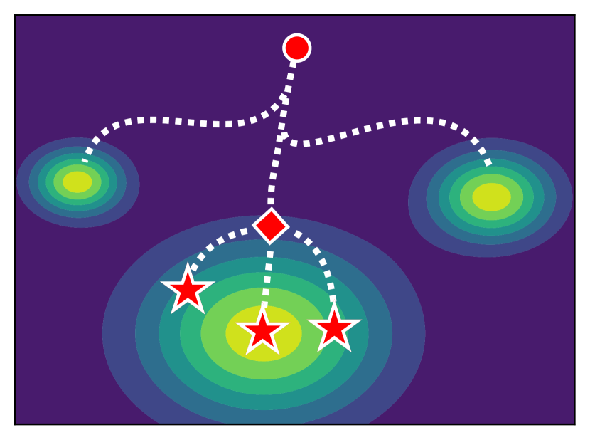
Figure 5: Mode Determinism: As a training trajectory proceeds from the initialization point (pictured as the red circle here) its path may diverge to various minima in the loss landscape due to SGD noise (e.g., batch order) or changes in the underlying data distribution, but after a certain number of steps the trajectory of a model reaches a stable point (pictured as the red diamond). Any further fine-tuning from this point onwards, even on slightly different data distributions, will result in models lying in the same convex objective basin (red stars).

Mode Determinism: The final linearly connected objective basin to which deep learning models converge is determined early in the training process. This assertion is supported by experiments on linear connectivity [47] and by visualizations of model clustering in parameter space [82]. SGD has been observed to occur in two phases: an initial period of instability, followed by a more stable, linear trajectory [47, 120, 121, 122, 123, 124]. Fort et al. [62] show that this behavior corresponds to the expected dynamics of the Neural Tangent Kernel. Weight aggregation techniques implicitly use mode determinism; otherwise, they could not merge models using linear combinations of their parameters. Instead, we would expect barriers of high loss between models that were independently fine-tuned. Linearly connected models also demonstrate linearity in their features—that is, linear interpolations between their parameters correspond to linear interpolations between their feature maps [39, 111]. This result implies that the nature of the representations that models will learn is also determined early in the training process. Damian et al. [121] explain the stability in the later part of the training trajectory for neural networks by the tendency of SGD to implicitly regularize the sharpness of the loss landscape. They demonstrate the explicit presence of such a regularization term in the Taylor expansion of the SGD update equation. This result suggests that the observed stability in the training trajectory is a property of SGD itself.

Mode Directedness: Within a given objective basin, we can meaningfully associate directions in parameter space with task-specific behavior. This “directedness” is best illustrated by the success of methods such as Task Arithmetic [85]. Follow-up work, such as TIES-merging [88] and DARE [89], demonstrate that removing redundancies and low-magnitude differences between task vectors improves merging performance. This implies that just a few principal directions can effectively account for task-specific behavior. Gueta et al. [82] demonstrate the clustering behavior of language models trained on similar tasks. They observe that models trained on the same dataset are tightly clustered in parameter space, whereas models trained on the same underlying task with different datasets form looser clusters. This notion of hierarchically organized task-specific areas in parameter space offers an explanation for the success of several standard routines in the contemporary deep learning landscape, including the pre-train fine-tune training paradigm and meta-learning procedures such as Model-Agnostic Meta-Learning [125]. These procedures may move parameters into regions of space where effective parameter configurations for more specialized sub-tasks are abundant. While the existence of meaningful task-specific regions in space has been proposed previously to motivate meta-learning approaches, the merging literature justifies these conjectures with empirical evidence showing that this kind of organization is present at multiple scales.

Mode Connectivity: Even solutions found in distinct objective modes can be connected by low-loss paths that are comprised of equally performant solutions. Moreover, this connectivity between solutions in separate modes is commonplace, as is LMC, i.e., the presence of linear paths of low loss between known solutions in objective space. There may even be entire manifolds of low loss connecting equally performant solutions [72]. An accumulation of evidence suggests that models trained on similar tasks, even with different initializations, can be connected by paths of low loss if one accounts for the inherent permutation invariance of neural networks by appropriately aligning their parameters after training [16, 19, 20, 47, 51]. Additionally, Li et al. [57] showcase how constraining training of a network to a subspace or pruning prior to training reduces the number of inherent permutation symmetries and leads to LMC between solutions without further post-training alignment. This result implies that constraining neuron misalignment from arising can enable the discovery of connected paths between modes more easily.

Several theoretical results suggest that the loss landscape of overparameterized models is dominated by subspaces of permutation-equivalent objective basins [55]. This observation suggests that model representations are generally quite similar—even under different forms of SGD noise or initializations, they tend to converge to similar solutions. This similarity may be even more prevalent as models are further over-parameterized, offering an explanation for why merging methods are often more successful as model size increases.

VII-B Implications for Model Training

The direct comparison of model representations in merging studies allows us to derive information about the effects of model architecture and pre-training objectives on learned representations. Here, we outline some of these findings.

Model Size: Neuron alignment procedures struggle as model width decreases. Ito et al. [59] investigate this phenomenon by studying the distribution of singular values in the weight matrices of source models. They conjecture that the effectiveness of neuron alignment techniques is predicated on their ability to align preferentially the singular directions corresponding to dominant singular values. They find that the proportion of dominant singular values decreases substantially as model width increases, suggesting that wider models are easier to align. Nguyen et al. [117] show empirical results suggesting that over-parameterized models propagate dominant principal components of their hidden representations at each layer. These results support the idea that a few dominant feature directions arise in over-parameterized models.

Aghajanyan et al. [15] measure the intrinsic dimensionality of language models and similarly conclude that LLMs form more compressed representations as they scale in size. These works suggest that larger models, despite their increased expressiveness, have fewer dominant directions in feature space. Some work has also attempted to clarify why over-parameterized models may display more amicable optimization behavior than smaller models. Huang et al. [66] and Li et al. [14] visualize the loss landscapes of models at various sizes and find that overparameterized models often converge to large, flat basins correlated with enhanced generalization capability [64, 66, 67, 68, 69, 126, 127] as opposed to small sharp minima. They explain this tendency by observing that such basins occupy far more volume in objective space as the dimensionality of a model increases. The increased volume of flat basins, coupled with the results presented by Simsek et al. [55] indicating that the number of permutation-equivalent basins increases exponentially as models grow in size, may explain the relative ease with which large models train: the volume of objective space corresponding to good solutions grows exponentially with model size.

Figure 6: Mode Directedness: Optimal parameter settings for related tasks lie clustered together in parameter space; clusters become looser as tasks diverge in similarity. This suggests a hierarchical organization of the objective landscape with respect to semantically similar tasks.

Pre-training Objective: Models with different pre-training objectives display different sensitivities to various merging techniques [21, 26]. For example, transformer models in the T5 family [128] perform well even with only simple averaging; meanwhile, DeBERTa models [129] consistently degrade in performance when merged, even when using state-of-the-art techniques [21]. This discrepancy points to an interplay between the pre-training objective and the success of model merging procedures. One possible explanation for this difference is the effect of pre-training objective on training dynamics. Some evidence suggests a strong link between a model’s pre-training objective and the final objective basin in which it lies—for example, contrastive pre-training has been observed to coerce models to lie in flatter objective basins associated with better generalization and robustness guarantees [38]. Certain pre-training procedures seem to predispose models toward representations that display linear connectivity and linear relationships between activations [21, 111]. Understanding this interaction is important for interpretability work that seeks to isolate task-specific behavior [130, 131, 132] or to disentangle and identify key directions in latent space [133]. Some work has explored the overlap between pre-training objective, loss landscape geometry, and adversarial robustness [38, 134]. Further work might consider the causal effects of pre-training objective on loss landscape geometry and relate it to resulting model robustness and performance in downstream tasks.

VIII Discussion

Model merging is closely tied to model interpretability. Techniques in interpretability research, such as activation steering, can control language style, reduce model toxicity, and edit factual associations post-training [135, 136]. Such methods involve altering model behavior via linear changes to the activation space [137]. Existing work on task arithmetic [85], TIES-merging [88], and AdaMerge [97] demonstrates the viability of this approach to model steering by showcasing the linear correspondence between changes in model activations and changes in model weights [39, 111]. Model merging techniques provide valuable insights into the mutable nature of hidden representations and their connection to model parameters. The linearity of feature representations implies that cheap interventions on model weights can replicate such procedures—circumventing the need to apply activation steering methods that require extensive tuning [135, 136].

Interpretability studies should focus on groups of models. Model merging literature highlights that machine learning practitioners have the tools to localize task-specific behaviors to specific model components (e.g., layers, neurons, weights). These localization tools can enable researchers to interpret how a model learns information. Conventionally, interpretability studies seek to understand the underlying mechanics of individual models [29, 96, 130, 131, 137, 138]; however, this paradigm is limiting.

We propose that studying groups of models, as done in the model merging literature, would more easily enable researchers to make substantial claims about how common behaviors (e.g., memorization) arise across families of models. Interpretability work can draw upon insights from the model merging literature, for instance: (i) models trained on similar tasks can be aligned to find common subsets of parameters for a given task [19, 20, 101]; (ii) models trained on different randomly chosen subsets of data or different hyperparameters when merged can help identify parts of the models that are relevant to the overall task invariant to the specific data or hyperparameters that was used to train the model [78, 79, 83, 101]; and (iii) models with similar underlying training distributions cluster together in parameter space [82].

For example, to study the behavior of memorization in LLMs, we argue that it is easier to glean insights into how a model learns that behavior by studying how (and if) it arises in a group of models with variations in their training recipes (as opposed to studying a single model exhibiting memorization). Methods such as ZipIt! [101] showcase how we can distinguish parameters associated with differences in behavior between models. We can also find new interventions on model parameters using notions of loss landscape geometry. For example, Barbulescu and Triantafillou [30] demonstrate how to use Task Arithmetic to unlearn memorized data. We can imagine similar interventions that also consider the mode-directedness of the objective landscape—perhaps identifying whole regions of parameter space that are more prone to degenerate behavior like memorization, and developing train-time mitigations to prevent their development.

The fundamental unit of analysis in neural networks. The discussion in this paper focuses predominantly on merging weights. However, much analysis of neural networks is done in activation space. What the correct unit of analysis is in neural networks is an open question. Neurons are the most natural choice for analysis due to their simplicity. However, rigorous examinations show that natural language explanations for neuron activation patterns systematically display poor precision and recall while also failing to behave as expected under causal interventions [139]. Elhage et al. [140] propose that neural networks represent concepts in “superposition.” That is, rather than having meaningful concepts axis-aligned in their hidden states, neural networks pack many almost orthogonal concepts into the high dimensional space defined by the neurons. This idea has led researchers to focus on analysis in linear directions [141], polytopes [142], and subspaces [143] in the activation space. Dictionary learning [144] and sparse autoencoders [133, 145] identify meaningful directions in the hidden states of neural networks in an unsupervised fashion—both methods learn compressed representations of hidden states by producing sparse reconstructions of them. Ideally, these representations would correspond to interpretable concepts. However, Chaudhary and Geiger [146] find that the features learned by sparse autoencoders perform worse than neuron-level features under causal interventions on a benchmark dataset.

Geiger et al. [95] propose Distributed Alignment Search, a supervised method that learns a rotation matrix that rotates the hidden states of a neural network so that the trained features are axis-aligned. Intuitively, this shows that meaningful features correspond to directions in the hidden state, but these features are not automatically aligned to the axes defined by the neurons. Each of these methods relies on the intuition that the structure of what a neural network has learned is encoded in the geometry of the activation space. Most activation steering work alters activations [29, 137] and relies on the intuition that directions in activation space are the fundamental unit of analysis of neural networks. The model merging literature suggests that directions in weight space may also be appropriate for model steering and analysis.

Advancements in model security depend on a rich understanding of loss landscape geometry. Mode determinism and mode directedness are implicitly or explicitly applied in various attacks on deep learning models. In black-box scenarios, it is common to train local substitute models of a similar architecture on training data for the same underlying task to develop adversarial samples [147, 148]. This assumption of similarity in learned representation and behavior is encapsulated by the concept of mode directedness and is supported by the model merging and loss landscape literature. Many attacks, such as data poisoning and membership inference, can be aided by training similar models on similar data distributions [9]. Mode determinism implies that such attacks may be especially effective when deployed against freely available pre-trained checkpoints, as fine-tuned models will likely be even closer in their representations [47, 82].

The study of model security is increasingly dependent on an understanding of loss landscape geometry [149, 40]. For example, the success of gradient obfuscation against gradient-based adversaries has been linked to how gradient obfuscation alters the local loss landscape geometry—making it difficult to ascend for adversaries. Conversely, this insight led to the development of a countermeasure that enables adversaries to effectively mitigate defenses based on gradient obfuscation by navigating an altered loss geometry [150]. Train-time defenses against adversarial examples frequently involve navigating towards robust local minima via the addition of an adversarial robustness term—one can even thwart subsequent fine-tuning success in restricted domains by appropriate engineering of the loss function [134]. This has been observed to bias models toward large, flat loss basins. Indeed, a strong correlation has been established between adversarial robustness and local loss curvature, indicating that solutions in large, flat basins are more robust to adversaries [149].

Furthermore, the locally convex, globally connected geometry of objective landscapes offers a framework from which defenses may arise. Gradient obfuscation and other schemes that sample model parameters from a distribution implicitly use local convexity in objective basins by sampling predictions from nearby models. Some works have even explicitly exploited mode connectivity to learn paths between vulnerable solutions that contain more robust models—outperforming fine-tuning in terms of model robustness and accuracy [149]. This underscores the advancements that a deep understanding of loss landscape geometry may yield in model security.

IX Conclusion & Future Work

We have surveyed a range of model merging techniques and extracted insights from their empirical observations to characterize several aspects of the underlying structure of loss landscapes—namely mode convexity, mode determinism, mode directedness, and mode connectivity. We discussed the intimate connections between these observations and model interpretability and security, offering analogs for traditional activation space analysis in weight space.

Future work exploring the intersection of these fields might focus on understanding the relationship between the objective geometry of hierarchically related tasks, with the goal of understanding why semantically similar tasks produce solutions close together in parameter space, even when their raw data distributions (over, say, tokens) might seem quite dissimilar in principle [82]. Such investigations would touch on the ability of neural networks to abstract and generalize across tasks in a meaningful way. One could also attempt to “orthogonalize” task-specific directions in weight space to obtain interpretable decompositions over directions in parameter space as an alternative to activation-based methods. Other extensions might further explore methods for continual learning, few-shot learning, or parameter-efficient fine-tuning through model merging techniques.

A concerning implication of our work is that, due to the principle of mode determinism, models fine-tuned from pre-trained checkpoints—particularly those fine-tuned on similar tasks—will have similar representations and lie close together in parameter space. Therefore, models stemming from freely available pre-trained checkpoints might be especially vulnerable to adversaries attempting to replicate model behavior [9, 147, 148]. This could lead to problems, given that the dominant paradigm for model deployment is currently predicated on extensive pre-training and domain-specific fine-tuning.

References

- Kalyan et al. [2021] K. S. Kalyan, A. Rajasekharan, and S. Sangeetha, “AMMUS: A survey of transformer-based pretrained models in natural language processing,” arXiv preprint arXiv:2108.05542, 2021.
- Liu et al. [2023] Y. Liu, Y. Zhang, Y. Wang, F. Hou, J. Yuan, J. Tian, Y. Zhang, Z. Shi, J. Fan, and Z. He, “A survey of visual transformers,” IEEE Transactions on Neural Networks and Learning Systems, 2023.
- Torres et al. [2021] J. F. Torres, D. Hadjout, A. Sebaa, F. Martínez-Álvarez, and A. Troncoso, “Deep learning for time series forecasting: A survey,” Big Data, vol. 9, no. 1, pp. 3–21, 2021.
- Ahmed et al. [2023] M. I. Ahmed, B. Spooner, J. Isherwood, M. Lane, E. Orrock, and A. Dennison, “A systematic review of the barriers to the implementation of artificial intelligence in healthcare,” Cureus, vol. 15, no. 10, 2023.
- Muhammad et al. [2020] K. Muhammad, A. Ullah, J. Lloret, J. Del Ser, and V. H. C. de Albuquerque, “Deep learning for safe autonomous driving: Current challenges and future directions,” IEEE Transactions on Intelligent Transportation Systems, vol. 22, no. 7, pp. 4316–4336, 2020.
- Hall and Agarwal [2024] A. Hall and V. Agarwal, “Barriers to adopting artificial intelligence and machine learning technologies in nuclear power,” Progress in Nuclear Energy, vol. 175, p. 105295, 2024.
- Ji et al. [2023] Z. Ji, N. Lee, R. Frieske, T. Yu, D. Su, Y. Xu, E. Ishii, Y. J. Bang, A. Madotto, and P. Fung, “Survey of hallucination in natural language generation,” ACM Computing Surveys, vol. 55, no. 12, pp. 1–38, 2023.
- Mirsky and Lee [2021] Y. Mirsky and W. Lee, “The creation and detection of deepfakes: A survey,” ACM computing surveys (CSUR), vol. 54, no. 1, pp. 1–41, 2021.
- Shokri et al. [2017] R. Shokri, M. Stronati, C. Song, and V. Shmatikov, “Membership inference attacks against machine learning models,” in IEEE Symposium on Security and Privacy. IEEE, 2017, pp. 3–18.
- Zhu et al. [2019] L. Zhu, Z. Liu, and S. Han, “Deep leakage from gradients,” Advances in neural information processing systems, vol. 32, 2019.
- Maini et al. [2023] P. Maini, M. C. Mozer, H. Sedghi, Z. C. Lipton, J. Z. Kolter, and C. Zhang, “Can neural network memorization be localized?” arXiv preprint arXiv:2307.09542, 2023.
- Shah and Sureja [2024] M. Shah and N. Sureja, “A comprehensive review of bias in deep learning models: Methods, impacts, and future directions,” Archives of Computational Methods in Engineering, pp. 1–13, 2024.
- Haim et al. [2024] A. Haim, A. Salinas, and J. Nyarko, “What’s in a name? Auditing large language models for race and gender bias,” arXiv preprint arXiv:2402.14875, 2024.
- Li et al. [2018a] C. Li, H. Farkhoor, R. Liu, and J. Yosinski, “Measuring the intrinsic dimension of objective landscapes,” arXiv preprint arXiv:1804.08838, 2018.
- Aghajanyan et al. [2020] A. Aghajanyan, L. Zettlemoyer, and S. Gupta, “Intrinsic dimensionality explains the effectiveness of language model fine-tuning,” arXiv preprint arXiv:2012.13255, 2020.
- Entezari et al. [2021] R. Entezari, H. Sedghi, O. Saukh, and B. Neyshabur, “The role of permutation invariance in linear mode connectivity of neural networks,” arXiv preprint arXiv:2110.06296, 2021.
- Arous et al. [2023] G. B. Arous, R. Gheissari, J. Huang, and A. Jagannath, “High-dimensional SGD aligns with emerging outlier eigenspaces,” arXiv preprint arXiv:2310.03010, 2023.
- Chaudhry et al. [2020] A. Chaudhry, N. Khan, P. Dokania, and P. Torr, “Continual learning in low-rank orthogonal subspaces,” Advances in Neural Information Processing Systems, vol. 33, pp. 9900–9911, 2020.
- Ainsworth et al. [2022] S. K. Ainsworth, J. Hayase, and S. Srinivasa, “Git Re-Basin: Merging models modulo permutation symmetries,” arXiv preprint arXiv:2209.04836, 2022.
- Singh and Jaggi [2020] S. P. Singh and M. Jaggi, “Model fusion via optimal transport,” Advances in Neural Information Processing Systems, vol. 33, pp. 22 045–22 055, 2020.
- Jin et al. [2022] X. Jin, X. Ren, D. Preotiuc-Pietro, and P. Cheng, “Dataless knowledge fusion by merging weights of language models,” arXiv preprint arXiv:2212.09849, 2022.
- Yamada et al. [2023] M. Yamada, T. Yamashita, S. Yamaguchi, and D. Chijiwa, “Revisiting permutation symmetry for merging models between different datasets,” arXiv preprint arXiv:2306.05641, 2023.
- Yao et al. [2022] H. Yao, C. Choi, B. Cao, Y. Lee, P. W. W. Koh, and C. Finn, “Wild-time: A benchmark of in-the-wild distribution shift over time,” Advances in Neural Information Processing Systems, vol. 35, pp. 10 309–10 324, 2022.
- Lin et al. [2024] V. Lin, K. J. Jang, S. Dutta, M. Caprio, O. Sokolsky, and I. Lee, “DC4L: Distribution shift recovery via data-driven control for deep learning models,” in 6th Annual Learning for Dynamics & Control Conference. PMLR, 2024, pp. 1526–1538.
- Matena and Raffel [2022] M. S. Matena and C. A. Raffel, “Merging models with Fisher-weighted averaging,” Advances in Neural Information Processing Systems, vol. 35, pp. 17 703–17 716, 2022.
- Tam et al. [2023] D. Tam, M. Bansal, and C. Raffel, “Merging by matching models in task subspaces,” arXiv preprint arXiv:2312.04339, 2023.
- McMahan et al. [2017] B. McMahan, E. Moore, D. Ramage, S. Hampson, and B. A. y Arcas, “Communication-efficient learning of deep networks from decentralized data,” in Artificial intelligence and statistics. PMLR, 2017, pp. 1273–1282.
- Clark et al. [2019] K. Clark, U. Khandelwal, O. Levy, and C. D. Manning, “What does BERT look at? an analysis of BERT’s attention,” arXiv preprint arXiv:1906.04341, 2019.
- Turner et al. [2023] A. M. Turner, L. Thiergart, G. Leech, D. Udell, J. J. Vazquez, U. Mini, and M. MacDiarmid, “Activation addition: Steering language models without optimization,” arXiv preprint arXiv:2308.10248, 2023.
- Barbulescu and Triantafillou [2024] G.-O. Barbulescu and P. Triantafillou, “To each (textual sequence) its own: Improving memorized-data unlearning in large language models,” arXiv preprint arXiv:2405.03097, 2024.
- Finlayson et al. [2019] S. G. Finlayson, J. D. Bowers, J. Ito, J. L. Zittrain, A. L. Beam, and I. S. Kohane, “Adversarial attacks on medical machine learning,” Science, vol. 363, no. 6433, pp. 1287–1289, 2019.
- Li et al. [2021] Q. Li, Z. Wen, Z. Wu, S. Hu, N. Wang, Y. Li, X. Liu, and B. He, “A survey on federated learning systems: Vision, hype and reality for data privacy and protection,” IEEE Transactions on Knowledge and Data Engineering, vol. 35, no. 4, pp. 3347–3366, 2021.
- Bogdanova et al. [2020] A. Bogdanova, N. Attoh-Okine, and T. Sakurai, “Risk and advantages of federated learning for health care data collaboration,” ASCE-ASME Journal of Risk and Uncertainty in Engineering Systems, Part A: Civil Engineering, vol. 6, no. 3, p. 04020031, 2020.
- Dimitrov et al. [2022] D. I. Dimitrov, M. Balunovic, N. Konstantinov, and M. Vechev, “Data leakage in federated averaging,” Transactions on Machine Learning Research, 2022.
- Kuo and Pham [2022] T.-T. Kuo and A. Pham, “Detecting model misconducts in decentralized healthcare federated learning,” International Journal of Medical Informatics, vol. 158, p. 104658, 2022.
- Darzi et al. [2023] E. Darzi, N. M. Sijtsema, and P. van Ooijen, “Fed-Safe: Securing federated learning in healthcare against adversarial attacks,” arXiv preprint arXiv:2310.08681, 2023.
- Zhang and Li [2019] J. Zhang and C. Li, “Adversarial examples: Opportunities and challenges,” IEEE transactions on neural networks and learning systems, vol. 31, no. 7, pp. 2578–2593, 2019.
- Fradkin et al. [2022] P. Fradkin, L. Atanackovic, and M. R. Zhang, “Robustness to adversarial gradients: A glimpse into the loss landscape of contrastive pre-training,” in First Workshop on Pre-training: Perspectives, Pitfalls, and Paths Forward at ICML 2022, 2022.
- Zhou et al. [2023] Z. Zhou, Y. Yang, X. Yang, J. Yan, and W. Hu, “Going beyond linear mode connectivity: The layerwise linear feature connectivity,” Advances in Neural Information Processing Systems, vol. 36, pp. 60 853–60 877, 2023.
- Xu et al. [2019] J. Xu, D. A. Yap, and V. U. Prabhu, “Understanding adversarial robustness through loss landscape geometries,” in Proc. of the International Conference on Machine Learning (ICML) Workshops, vol. 18, 2019.
- Li et al. [2024a] L. Li, J. Gou, B. Yu, L. Du, and Z. Y. D. Tao, “Federated distillation: A survey,” arXiv preprint arXiv:2404.08564, 2024.
- Yadav et al. [2024a] P. Yadav, C. Raffel, M. Muqeeth, L. Caccia, H. Liu, T. Chen, M. Bansal, L. Choshen, and A. Sordoni, “A survey on model MoErging: Recycling and routing among specialized experts for collaborative learning,” arXiv preprint arXiv:2408.07057, 2024.
- Li et al. [2023] W. Li, Y. Peng, M. Zhang, L. Ding, H. Hu, and L. Shen, “Deep model fusion: A survey,” arXiv preprint arXiv:2309.15698, 2023.
- Yang et al. [2024] E. Yang, L. Shen, G. Guo, X. Wang, X. Cao, J. Zhang, and D. Tao, “Model merging in LLMs, MLLMs, and beyond: Methods, theories, applications and opportunities,” arXiv preprint arXiv:2408.07666, 2024.
- Li et al. [2018b] H. Li, Z. Xu, G. Taylor, C. Studer, and T. Goldstein, “Visualizing the loss landscape of neural nets,” Advances in Neural Information Processing Systems, vol. 31, 2018.
- Draxler et al. [2018] F. Draxler, K. Veschgini, M. Salmhofer, and F. Hamprecht, “Essentially no barriers in neural network energy landscape,” in International Conference on Machine Learning. PMLR, 2018, pp. 1309–1318.
- Frankle et al. [2020] J. Frankle, G. K. Dziugaite, D. Roy, and M. Carbin, “Linear mode connectivity and the lottery ticket hypothesis,” in International Conference on Machine Learning. PMLR, 2020, pp. 3259–3269.
- Nagarajan and Kolter [2019] V. Nagarajan and J. Z. Kolter, “Uniform convergence may be unable to explain generalization in deep learning,” Advances in Neural Information Processing Systems, vol. 32, 2019.
- Juneja et al. [2022] J. Juneja, R. Bansal, K. Cho, J. Sedoc, and N. Saphra, “Linear connectivity reveals generalization strategies,” arXiv preprint arXiv:2205.12411, 2022.
- Garipov et al. [2018] T. Garipov, P. Izmailov, D. Podoprikhin, D. P. Vetrov, and A. G. Wilson, “Loss surfaces, mode connectivity, and fast ensembling of DNNs,” Advances in Neural Information Processing systems, vol. 31, 2018.
- Tatro et al. [2020] N. Tatro, P.-Y. Chen, P. Das, I. Melnyk, P. Sattigeri, and R. Lai, “Optimizing mode connectivity via neuron alignment,” Advances in Neural Information Processing Systems, vol. 33, pp. 15 300–15 311, 2020.
- Tan et al. [2023] C. Tan, T. Long, S. Zhao, and R. Laine, “Geodesic mode connectivity,” arXiv preprint arXiv:2308.12666, 2023.
- Qin et al. [2022] Y. Qin, C. Qian, J. Yi, W. Chen, Y. Lin, X. Han, Z. Liu, M. Sun, and J. Zhou, “Exploring mode connectivity for pre-trained language models,” arXiv preprint arXiv:2210.14102, 2022.
- Zhou et al. [2024a] Z. Zhou, Z. Chen, Y. Chen, B. Zhang, and J. Yan, “On the emergence of cross-task linearity in pretraining-finetuning paradigm,” in Forty-first International Conference on Machine Learning, 2024. [Online]. Available: https://openreview.net/forum?id=qg6AlnpEQH
- Simsek et al. [2021] B. Simsek, F. Ged, A. Jacot, F. Spadaro, C. Hongler, W. Gerstner, and J. Brea, “Geometry of the loss landscape in overparameterized neural networks: Symmetries and invariances,” in International Conference on Machine Learning. PMLR, 2021, pp. 9722–9732.
- Brea et al. [2019] J. Brea, B. Simsek, B. Illing, and W. Gerstner, “Weight-space symmetry in deep networks gives rise to permutation saddles, connected by equal-loss valleys across the loss landscape,” arXiv preprint arXiv:1907.02911, 2019.
- Li et al. [2024b] Z. Li, Z. Li, J. Lin, T. Shen, T. Lin, and C. Wu, “Training-time neuron alignment through permutation subspace for improving linear mode connectivity and model fusion,” arXiv preprint arXiv:2402.01342, 2024.
- Wang et al. [2020a] H. Wang, M. Yurochkin, Y. Sun, D. Papailiopoulos, and Y. Khazaeni, “Federated learning with matched averaging,” arXiv preprint arXiv:2002.06440, 2020.
- Ito et al. [2024] A. Ito, M. Yamada, and A. Kumagai, “Analysis of linear mode connectivity via permutation-based weight matching,” arXiv preprint arXiv:2402.04051, 2024.
- Vergara-Browne et al. [2024] T. Vergara-Browne, Á. Soto, and A. Aizawa, “Eigenpruning,” arXiv preprint arXiv:2404.03147, 2024.
- Nakhodnov et al. [2022] M. S. Nakhodnov, M. S. Kodryan, E. M. Lobacheva, and D. S. Vetrov, “Loss function dynamics and landscape for deep neural networks trained with quadratic loss,” in Doklady Mathematics, vol. 106, no. Suppl 1. Springer, 2022, pp. S43–S62.
- Fort et al. [2020] S. Fort, G. K. Dziugaite, M. Paul, S. Kharaghani, D. M. Roy, and S. Ganguli, “Deep learning versus kernel learning: An empirical study of loss landscape geometry and the time evolution of the neural tangent kernel,” Advances in Neural Information Processing Systems, vol. 33, pp. 5850–5861, 2020.
- Mienye and Sun [2022] I. D. Mienye and Y. Sun, “A survey of ensemble learning: Concepts, algorithms, applications, and prospects,” IEEE Access, vol. 10, pp. 99 129–99 149, 2022.
- Izmailov et al. [2018] P. Izmailov, D. Podoprikhin, T. Garipov, D. Vetrov, and A. G. Wilson, “Averaging weights leads to wider optima and better generalization,” arXiv preprint arXiv:1803.05407, 2018.
- Hoeting [1999] J. A. Hoeting, “Bayesian model averaging: A tutorial,” Statistical Science, vol. 14, no. 4, pp. 382–417, 1999.
- Huang et al. [2020] W. R. Huang, Z. Emam, M. Goldblum, L. Fowl, J. K. Terry, F. Huang, and T. Goldstein, “Understanding generalization through visualizations,” Proceedings of Machine Learning Research, 2020.
- Chaudhari et al. [2019] P. Chaudhari, A. Choromanska, S. Soatto, Y. LeCun, C. Baldassi, C. Borgs, J. Chayes, L. Sagun, and R. Zecchina, “Entropy-SGD: Biasing gradient descent into wide valleys,” Journal of Statistical Mechanics: Theory and Experiment, vol. 2019, no. 12, p. 124018, 2019.
- Hochreiter and Schmidhuber [1997] S. Hochreiter and J. Schmidhuber, “Flat minima,” Neural computation, vol. 9, no. 1, pp. 1–42, 1997.
- Keskar et al. [2016] N. S. Keskar, D. Mudigere, J. Nocedal, M. Smelyanskiy, and P. T. P. Tang, “On large-batch training for deep learning: Generalization gap and sharp minima,” arXiv preprint arXiv:1609.04836, 2016.
- Lakshminarayanan et al. [2017] B. Lakshminarayanan, A. Pritzel, and C. Blundell, “Simple and scalable predictive uncertainty estimation using deep ensembles,” Advances in Neural Information Processing Systems, vol. 30, 2017.
- Huang et al. [2017] G. Huang, Y. Li, G. Pleiss, Z. Liu, J. E. Hopcroft, and K. Q. Weinberger, “Snapshot ensembles: Train 1, get m for free,” arXiv preprint arXiv:1704.00109, 2017.
- Benton et al. [2021] G. Benton, W. Maddox, S. Lotfi, and A. G. G. Wilson, “Loss surface simplexes for mode connecting volumes and fast ensembling,” in International Conference on Machine Learning. PMLR, 2021, pp. 769–779.
- Masoudnia and Ebrahimpour [2014] S. Masoudnia and R. Ebrahimpour, “Mixture of experts: A literature survey,” Artificial Intelligence Review, vol. 42, pp. 275–293, 2014.
- Akiba et al. [2024] T. Akiba, M. Shing, Y. Tang, Q. Sun, and D. Ha, “Evolutionary optimization of model merging recipes,” arXiv preprint arXiv:2403.13187, 2024.
- Pan et al. [2024] B. Pan, Y. Shen, H. Liu, M. Mishra, G. Zhang, A. Oliva, C. Raffel, and R. Panda, “Dense training, sparse inference: Rethinking training of mixture-of-experts language models,” arXiv preprint arXiv:2404.05567, 2024.
- Hinne et al. [2020] M. Hinne, Q. F. Gronau, D. van den Bergh, and E.-J. Wagenmakers, “A conceptual introduction to Bayesian model averaging,” Advances in Methods and Practices in Psychological Science, vol. 3, no. 2, pp. 200–215, 2020.
- Erhan et al. [2010] D. Erhan, A. Courville, Y. Bengio, and P. Vincent, “Why does unsupervised pre-training help deep learning?” in 13th International Conference on Artificial Intelligence and Statistics. JMLR Workshop and Conference Proceedings, 2010, pp. 201–208.
- Wortsman et al. [2022] M. Wortsman, G. Ilharco, S. Y. Gadre, R. Roelofs, R. Gontijo-Lopes, A. S. Morcos, H. Namkoong, A. Farhadi, Y. Carmon, S. Kornblith, and L. Schmidt, “Model soups: Averaging weights of multiple fine-tuned models improves accuracy without increasing inference time,” in International Conference on Machine Learning. PMLR, 2022, pp. 23 965–23 998.
- Zimmer et al. [2023] M. Zimmer, C. Spiegel, and S. Pokutta, “Sparse model soups: A recipe for improved pruning via model averaging,” arXiv preprint arXiv:2306.16788, 2023.
- Tanaka et al. [2020] H. Tanaka, D. Kunin, D. L. Yamins, and S. Ganguli, “Pruning neural networks without any data by iteratively conserving synaptic flow,” Advances in neural information processing systems, vol. 33, pp. 6377–6389, 2020.
- Choi et al. [2023] M. Choi, H. Lee, G. Nam, and J. Lee, “SWAMP: Sparse weight averaging with multiple particles for iterative magnitude pruning.” CoRR, 2023.
- Gueta et al. [2023] A. Gueta, E. Venezian, C. Raffel, N. Slonim, Y. Katz, and L. Choshen, “Knowledge is a region in weight space for fine-tuned language models,” arXiv preprint arXiv:2302.04863, 2023.
- Jang et al. [2024] D.-H. Jang, S. Yun, and D. Han, “Model stock: All we need is just a few fine-tuned models,” arXiv preprint arXiv:2403.19522, 2024.
- Wortsman et al. [2021] M. Wortsman, M. C. Horton, C. Guestrin, A. Farhadi, and M. Rastegari, “Learning neural network subspaces,” in International Conference on Machine Learning. PMLR, 2021, pp. 11 217–11 227.
- Ilharco et al. [2022a] G. Ilharco, M. T. Ribeiro, M. Wortsman, S. Gururangan, L. Schmidt, H. Hajishirzi, and A. Farhadi, “Editing models with task arithmetic,” arXiv preprint arXiv:2212.04089, 2022.
- Davari and Belilovsky [2023] M. Davari and E. Belilovsky, “Model breadcrumbs: Scaling multi-task model merging with sparse masks,” arXiv preprint arXiv:2312.06795, 2023.
- Ilharco et al. [2022b] G. Ilharco, M. Wortsman, S. Y. Gadre, S. Song, H. Hajishirzi, S. Kornblith, A. Farhadi, and L. Schmidt, “Patching open-vocabulary models by interpolating weights,” Advances in Neural Information Processing Systems, vol. 35, pp. 29 262–29 277, 2022.
- Yadav et al. [2024b] P. Yadav, D. Tam, L. Choshen, C. A. Raffel, and M. Bansal, “Ties-Merging: Resolving interference when merging models,” Advances in Neural Information Processing Systems, vol. 36, 2024.
- Yu et al. [2024] L. Yu, B. Yu, H. Yu, F. Huang, and Y. Li, “Language models are Super Mario: Absorbing abilities from homologous models as a free lunch,” in Forty-first International Conference on Machine Learning, 2024.
- Hu et al. [2021] E. J. Hu, Y. Shen, P. Wallis, Z. Allen-Zhu, Y. Li, S. Wang, L. Wang, and W. Chen, “LoRA: Low-rank adaptation of large language models,” arXiv preprint arXiv:2106.09685, 2021.
- Hayou et al. [2024] S. Hayou, N. Ghosh, and B. Yu, “LoRA+: Efficient low rank adaptation of large models,” arXiv preprint arXiv:2402.12354, 2024.
- Liu et al. [2024] S.-Y. Liu, C.-Y. Wang, H. Yin, P. Molchanov, Y.-C. F. Wang, K.-T. Cheng, and M.-H. Chen, “DoRA: Weight-decomposed low-rank adaptation,” arXiv preprint arXiv:2402.09353, 2024.
- Liu et al. [2022] H. Liu, D. Tam, M. Muqeeth, J. Mohta, T. Huang, M. Bansal, and C. A. Raffel, “Few-shot parameter-efficient fine-tuning is better and cheaper than in-context learning,” Advances in Neural Information Processing Systems, vol. 35, pp. 1950–1965, 2022.
- Wu et al. [2024a] Z. Wu, A. Arora, Z. Wang, A. Geiger, D. Jurafsky, C. D. Manning, and C. Potts, “ReFT: Representation finetuning for language models,” arXiv preprint arXiv:2404.03592, 2024.
- Geiger et al. [2024] A. Geiger, Z. Wu, C. Potts, T. Icard, and N. Goodman, “Finding alignments between interpretable causal variables and distributed neural representations,” in Causal Learning and Reasoning. PMLR, 2024, pp. 160–187.
- Wu et al. [2024b] Z. Wu, A. Geiger, T. Icard, C. Potts, and N. Goodman, “Interpretability at scale: Identifying causal mechanisms in alpaca,” Advances in Neural Information Processing Systems, vol. 36, 2024.
- Yang et al. [2023] E. Yang, Z. Wang, L. Shen, S. Liu, G. Guo, X. Wang, and D. Tao, “AdaMerging: Adaptive model merging for multi-task learning,” arXiv preprint arXiv:2310.02575, 2023.
- Zhao et al. [2024] Y. Zhao, W. Zhang, H. Wang, K. Kawaguchi, and L. Bing, “AdaMergeX: Cross-lingual transfer with large language models via adaptive adapter merging,” arXiv preprint arXiv:2402.18913, 2024.
- Wang et al. [2020b] D. Wang, E. Shelhamer, S. Liu, B. Olshausen, and T. Darrell, “Tent: Fully test-time adaptation by entropy minimization,” arXiv preprint arXiv:2006.10726, 2020.
- Liang et al. [2024] J. Liang, R. He, and T. Tan, “A comprehensive survey on test-time adaptation under distribution shifts,” International Journal of Computer Vision, pp. 1–34, 2024.
- Stoica et al. [2023] G. Stoica, D. Bolya, J. Bjorner, P. Ramesh, T. Hearn, and J. Hoffman, “ZipIt! Merging models from different tasks without training,” arXiv preprint arXiv:2305.03053, 2023.
- Xu et al. [2021] J. Xu, B. S. Glicksberg, C. Su, P. Walker, J. Bian, and F. Wang, “Federated learning for healthcare informatics,” Journal of healthcare informatics research, vol. 5, pp. 1–19, 2021.
- Hudson et al. [2022] N. Hudson, P. Oza, H. Khamfroush, and T. Chantem, “Smart edge-enabled traffic light control: Improving reward-communication trade-offs with federated reinforcement learning,” in IEEE International Conference on Smart Computing. IEEE, 2022, pp. 40–47.
- Hudson et al. [2021] N. Hudson, M. J. Hossain, M. Hosseinzadeh, H. Khamfroush, M. Rahnamay-Naeini, and N. Ghani, “A framework for edge intelligent smart distribution grids via federated learning,” in International Conference on Computer Communications and Networks. IEEE, 2021, pp. 1–9.
- Devaraj et al. [2024] H. Devaraj, S. Sohail, B. Li, N. Hudson, M. Baughman, K. Chard, R. Chard, E. Casella, I. Foster, and O. Rana, “RuralAI in tomato farming: Integrated sensor system, distributed computing and hierarchical federated learning for crop health monitoring,” IEEE Sensors Letters, 2024.
- Sun et al. [2022] T. Sun, D. Li, and B. Wang, “Decentralized federated averaging,” IEEE Transactions on Pattern Analysis and Machine Intelligence, vol. 45, no. 4, pp. 4289–4301, 2022.
- Martens and Grosse [2015] J. Martens and R. Grosse, “Optimizing neural networks with Kronecker-factored approximate curvature,” in International Conference on Machine Learning. PMLR, 2015, pp. 2408–2417.
- Grosse and Martens [2016] R. Grosse and J. Martens, “A Kronecker-factored approximate Fisher matrix for convolution layers,” in International Conference on Machine Learning. PMLR, 2016, pp. 573–582.
- Ba et al. [2017] J. Ba, R. B. Grosse, and J. Martens, “Distributed second-order optimization using kronecker-factored approximations.” in ICLR (Poster), 2017.
- Hestenes and Stiefel [1952] M. R. Hestenes and E. Stiefel, “Methods of conjugate gradients for solving linear systems,” Journal of Research of the National Bureau of Standards, vol. 49, no. 6, 1952.
- Zhou et al. [2024b] Z. Zhou, Z. Chen, Y. Chen, B. Zhang, and J. Yan, “Cross-task linearity emerges in the pretraining-finetuning paradigm,” arXiv preprint arXiv:2402.03660, 2024.
- Burkard and Cela [1999] R. E. Burkard and E. Cela, “Linear assignment problems and extensions,” in Handbook of combinatorial optimization: Supplement volume A. Springer, 1999, pp. 75–149.
- Kuhn [1955] H. W. Kuhn, “The Hungarian method for the assignment problem,” Naval research logistics quarterly, vol. 2, no. 1-2, pp. 83–97, 1955.
- Yurochkin et al. [2019] M. Yurochkin, M. Agarwal, S. Ghosh, K. Greenewald, N. Hoang, and Y. Khazaeni, “Bayesian nonparametric federated learning of neural networks,” in International Conference on Machine Learning. PMLR, 2019, pp. 7252–7261.
- Ziegler [2012] G. M. Ziegler, Lectures on polytopes. Springer Science & Business Media, 2012, vol. 152.
- Imfeld et al. [2023] M. Imfeld, J. Graldi, M. Giordano, T. Hofmann, S. Anagnostidis, and S. P. Singh, “Transformer fusion with optimal transport,” arXiv preprint arXiv:2310.05719, 2023.
- Nguyen et al. [2023] D. Nguyen, T. Nguyen, K. Nguyen, D. Phung, H. Bui, and N. Ho, “On cross-layer alignment for model fusion of heterogeneous neural networks,” in IEEE International Conference on Acoustics, Speech and Signal Processing. IEEE, 2023, pp. 1–5.
- Jordan et al. [2022] K. Jordan, H. Sedghi, O. Saukh, R. Entezari, and B. Neyshabur, “Repair: Renormalizing permuted activations for interpolation repair,” arXiv preprint arXiv:2211.08403, 2022.
- Zhao et al. [2020a] B. Zhao, K. R. Mopuri, and H. Bilen, “Dataset condensation with gradient matching,” arXiv preprint arXiv:2006.05929, 2020.
- Frankle and Carbin [2018] J. Frankle and M. Carbin, “The lottery ticket hypothesis: Finding sparse, trainable neural networks,” arXiv preprint arXiv:1803.03635, 2018.
- Damian et al. [2022] A. Damian, E. Nichani, and J. D. Lee, “Self-stabilization: The implicit bias of gradient descent at the edge of stability,” arXiv preprint arXiv:2209.15594, 2022.
- Fort et al. [2019] S. Fort, H. Hu, and B. Lakshminarayanan, “Deep ensembles: A loss landscape perspective,” arXiv preprint arXiv:1912.02757, 2019.
- Ma et al. [2022] C. Ma, D. Kunin, L. Wu, and L. Ying, “Beyond the quadratic approximation: The multiscale structure of neural network loss landscapes,” arXiv preprint arXiv:2204.11326, 2022.
- Cohen et al. [2021] J. Cohen, S. Kaur, Y. Li, J. Z. Kolter, and A. Talwalkar, “Gradient descent on neural networks typically occurs at the edge of stability,” in International Conference on Learning Representations, 2021.
- Finn et al. [2017] C. Finn, P. Abbeel, and S. Levine, “Model-agnostic meta-learning for fast adaptation of deep networks,” in International Conference on Machine Learning. PMLR, 2017, pp. 1126–1135.
- Dziugaite and Roy [2017] G. K. Dziugaite and D. M. Roy, “Computing nonvacuous generalization bounds for deep (stochastic) neural networks with many more parameters than training data,” arXiv preprint arXiv:1703.11008, 2017.
- Li et al. [2020] X. Li, Q. Gu, Y. Zhou, T. Chen, and A. Banerjee, “Hessian based analysis of SGD for deep nets: Dynamics and generalization,” in SIAM International Conference on Data Mining. SIAM, 2020, pp. 190–198.
- Raffel et al. [2020] C. Raffel, N. Shazeer, A. Roberts, K. Lee, S. Narang, M. Matena, Y. Zhou, W. Li, and P. J. Liu, “Exploring the limits of transfer learning with a unified text-to-text transformer,” Journal of Machine Learning Research, vol. 21, no. 140, pp. 1–67, 2020.
- He et al. [2020] P. He, X. Liu, J. Gao, and W. Chen, “DeBERTa: Decoding-enhanced BERT with disentangled attention,” arXiv preprint arXiv:2006.03654, 2020.
- Meng et al. [2022a] K. Meng, D. Bau, A. Andonian, and Y. Belinkov, “Locating and editing factual associations in GPT,” Advances in Neural Information Processing Systems, vol. 35, pp. 17 359–17 372, 2022.
- Meng et al. [2022b] K. Meng, A. S. Sharma, A. Andonian, Y. Belinkov, and D. Bau, “Mass-editing memory in a transformer,” arXiv preprint arXiv:2210.07229, 2022.
- Wortsman et al. [2019] M. Wortsman, A. Farhadi, and M. Rastegari, “Discovering neural wirings,” Advances in Neural Information Processing Systems, vol. 32, 2019.
- Bricken et al. [2023] T. Bricken, A. Templeton, J. Batson, B. Chen, A. Jermyn, T. Conerly, N. Turner, C. Anil, C. Denison, A. Askell, R. Lasenby, Y. Wu, S. Kravec, N. Schiefer, T. Maxwell, N. Joseph, A. Tamkin, K. Nguyen, B. McLean, J. E. Burke, T. Hume, S. Carter, T. Henighan, and C. Olah, “Towards monosemanticity: Decomposing language models with dictionary learning,” Transformer Circuits Thread, vol. 2, 2023.
- Deng et al. [2024] J. Deng, S. Pang, Y. Chen, L. Xia, Y. Bai, H. Weng, and W. Xu, “SOPHON: Non-fine-tunable learning to restrain task transferability for pre-trained models,” arXiv preprint arXiv:2404.12699, 2024.
- Konen et al. [2024] K. Konen, S. Jentzsch, D. Diallo, P. Schütt, O. Bensch, R. E. Baff, D. Opitz, and T. Hecking, “Style vectors for steering generative large language model,” arXiv preprint arXiv:2402.01618, 2024.
- Li et al. [2024c] Y. Li, Z. Wei, H. Jiang, and C. Gong, “DESTEIN: Navigating detoxification of language models via universal steering pairs and head-wise activation fusion,” arXiv preprint arXiv:2404.10464, 2024.
- Wang et al. [2024] T. Wang, X. Jiao, Y. He, Z. Chen, Y. Zhu, X. Chu, J. Gao, Y. Wang, and L. Ma, “Adaptive activation steering: A tuning-free LLM truthfulness improvement method for diverse hallucinations categories,” arXiv preprint arXiv:2406.00034, 2024.
- Conmy et al. [2023] A. Conmy, A. Mavor-Parker, A. Lynch, S. Heimersheim, and A. Garriga-Alonso, “Towards automated circuit discovery for mechanistic interpretability,” Advances in Neural Information Processing Systems, vol. 36, pp. 16 318–16 352, 2023.
- Huang et al. [2023] J. Huang, A. Geiger, K. D’Oosterlinck, Z. Wu, and C. Potts, “Rigorously assessing natural language explanations of neurons,” arXiv preprint arXiv:2309.10312, 2023.
- Elhage et al. [2022] N. Elhage, T. Hume, C. Olsson, N. Schiefer, T. Henighan, S. Kravec, Z. Hatfield-Dodds, R. Lasenby, D. Drain, C. Chen, R. Grosse, S. McCandlish, J. Kaplan, D. Amodei, M. Wattenberg, and C. Olah, “Toy models of superposition,” arXiv preprint arXiv:2209.10652, 2022.
- Park et al. [2023] K. Park, Y. J. Choe, and V. Veitch, “The linear representation hypothesis and the geometry of large language models,” arXiv preprint arXiv:2311.03658, 2023.
- Park et al. [2024] K. Park, Y. J. Choe, Y. Jiang, and V. Veitch, “The geometry of categorical and hierarchical concepts in large language models,” arXiv preprint arXiv:2406.01506, 2024.
- Engels et al. [2024] J. Engels, I. Liao, E. J. Michaud, W. Gurnee, and M. Tegmark, “Not all language model features are linear,” arXiv preprint arXiv:2405.14860, 2024.
- Olshausen and Field [1997] B. A. Olshausen and D. J. Field, “Sparse coding with an overcomplete basis set: A strategy employed by V1?” Vision research, vol. 37, no. 23, pp. 3311–3325, 1997.
- Huben et al. [2023] R. Huben, H. Cunningham, L. R. Smith, A. Ewart, and L. Sharkey, “Sparse autoencoders find highly interpretable features in language models,” in 12th International Conference on Learning Representations, 2023.
- Chaudhary and Geiger [2024] M. Chaudhary and A. Geiger, “Evaluating open-source sparse autoencoders on disentangling factual knowledge in GPT-2 small,” arXiv preprint arXiv:2409.04478, 2024.
- Papernot et al. [2017] N. Papernot, P. McDaniel, I. Goodfellow, S. Jha, Z. B. Celik, and A. Swami, “Practical black-box attacks against machine learning,” in Proceedings of the 2017 ACM on Asia conference on computer and communications security, 2017, pp. 506–519.
- Bhambri et al. [2019] S. Bhambri, S. Muku, A. Tulasi, and A. B. Buduru, “A survey of black-box adversarial attacks on computer vision models,” arXiv preprint arXiv:1912.01667, 2019.
- Zhao et al. [2020b] P. Zhao, P.-Y. Chen, P. Das, K. N. Ramamurthy, and X. Lin, “Bridging mode connectivity in loss landscapes and adversarial robustness,” arXiv preprint arXiv:2005.00060, 2020.
- Eustratiadis et al. [2022] P. Eustratiadis, H. Gouk, D. Li, and T. Hospedales, “Attacking adversarial defences by smoothing the loss landscape,” arXiv preprint arXiv:2208.00862, 2022.