Resonant Capture of Stars by Black Hole Binaries: Extreme Eccentricity Excitation
Abstract
Massive black hole (MBH) binaries in galactic nuclei are one of the leading sources of mHz gravitational waves (GWs) for future missions such as LISA. However, the poor sky localization of GW interferometers will make it challenging to identify the host galaxy of MBH mergers absent an electromagnetic counterpart. One such counterpart is the tidal disruption of a star that has been captured into mean motion resonance with the inspiraling binary. Here we investigate the production of tidal disruption events (TDEs) through capture into, and subsequent evolution in, orbital resonance. We examine the full nonlinear evolution of planar autoresonance for stars that lock in to autoresonance with a shrinking MBH binary. Capture into the 2:1 resonance is guaranteed for any realistic astrophysical parameters (given a relatively small MBH binary mass ratio), and the captured star eventually attains an eccentricity , leading to a TDE. Stellar disks can be produced around MBHs following an active galactic nucleus episode, and we estimate the TDE rates from resonant capture produced when a secondary MBH begins inspiralling through such a disk. In some cases, the last resonant TDE can occur within a decade of the eventual LISA signal, helping to localize the GW event.
keywords:
keyword1 – keyword2 – keyword31 Introduction
Astrophysical black holes are divided into three main categories – stellar mass black holes, intermediate mass black holes (IMBHs), and supermassive black holes (SMBHs). While there is extensive evidence for stellar mass black holes and SMBHs, the existence of IMBHs is still considered controversial, though there is growing observational evidence for them (e.g. Greene et al. 2020). IMBH candidates are most commonly claimed in dense star systems, either globular clusters or nuclear star clusters, and the search for them is a major challenge in high energy astrophysics, as their mass distribution would encode long-standing questions on the origins of SMBHs (Volonteri, 2010; Inayoshi et al., 2020).
One way to detect massive black holes (MBHs, a catchall term we will use to referr ot both IMBHs and SMBHs), is from electromagnetic flares generated by strong encounters with nearby stars. Near a MBH in a galactic nucleus, a star can be torn apart by tidal forces, producing a tidal disruption event (TDE). TDEs were first proposed theoretically decades ago (Hills, 1975; Rees, 1988), and since then have been observed, both in X-rays (Komossa & Bade, 1999; Komossa & Greiner, 1999) and in UV and visible light (Gezari et al., 2006, 2008; van Velzen et al., 2011)). Their radiation is very bright, characterized by a high-temperature quasi-thermal spectrum, which lasts for months (Arcavi et al., 2014; Hung et al., 2017; van Velzen et al., 2021) to years (van Velzen et al., 2019). TDEs are of astrophysical interest for a number of reasons; for example, they can be used as tools to measure black hole mass and spin (Mockler et al., 2019; Wen et al., 2020; Ryu et al., 2020; Wen et al., 2021); they may be the source of the highest-energy neutrinos seen by neutrino astrophysicists (Stein et al., 2021; Reusch et al., 2022); and lastly, they may be responsible for the growth of IMBHs and SMBHs (Milosavljević et al., 2006; Stone et al., 2017).
A related transient phenomena that occurs in galactic nuclei are EMRIs: extreme mass ratio in-spirals. When a small compact object orbits a massive one (say, a stellar black hole around a SMBH), it emits gravitational waves (GWs), causing its orbit to decay (Ryan, 1995; Sigurdsson & Rees, 1997). By measuring the GWs emitted during an EMRI, one can perform precision tests of general relativity (Amaro-Seoane, 2018), although this is ultimately a goal for the future, since the mHz GWs produced by EMRIs are too low in frequency to be seen by current ground-based detectors. However, in the near future, space-based laser interferometers such as LISA (Amaro-Seoane et al., 2022) and Taiji/TianQin (Luo et al., 2016; Ruan et al., 2020) will observe these GW signals. EMRI rates are highly uncertain, with current error bars on theoretical rate estimates spanning at least three orders of magnitude (Babak et al., 2017). The dynamical processes that produce EMRIs are varied, with multiple possible formation channels (Hopman & Alexander, 2005; Miller et al., 2005; Pan & Yang, 2021), but in general EMRIs are much less common than TDEs (Broggi et al., 2022).
In order for either a star to become a TDE or a compact object to become an EMRI, it needs to move into a highly eccentric orbit. In normal galaxies, this process is caused by an ensemble of weak 2-body scatterings from nearby stars, which leads to a random walk in orbital angular momentum (Frank & Rees, 1976; Cohn & Kulsrud, 1978). The rates of both TDEs and EMRIs, in this picture, are set by diffusion through phase space. The characteristic time length for this diffusion is quite long – in typical galaxies, TDEs are expected once every (Wang & Merritt, 2004; Stone & Metzger, 2016; van Velzen, 2018). Orbital diffusion to produce EMRIs has additional dynamical complexities (Bar-Or & Alexander, 2016; Qunbar & Stone, 2023), but is still a slow process. However, when the nucleus of a galaxy undergoes severe dynamical disturbances, the TDE rate can be elevated dramatically; one such example of a disturbance is the formation of a MBH binary.
MBH binaries most typically inspiral and merge in galactic nuclei. The canonical example of this occurs in the aftermath of a galaxy merger, when two MBHs sink to the center of the merged galaxy under the influence of dynamical friction (Begelman et al., 1980). Once the MBH binary becomes “hard,” i.e. the binary circular speed exceeds the local stellar velocity dispersion, dynamical friction becomes ineffective and the binary stalls for an extended period of time. As this happens for binary semimajor axes , this stalling is known as the “final parsec problem” (Begelman et al., 1980; Merritt & Milosavljević, 2005), and is only resolved once external forces reduce to scales of , where the (circular) GW inspiral time (Peters, 1964) is less than a Hubble time. Possible solutions to the final parsec problem include three-body scatterings with stars (Quinlan, 1996; Milosavljević & Merritt, 2001), which achieve high efficiency if the global potential of the galaxy is triaxial (Merritt & Poon, 2004; Vasiliev et al., 2015); secular or chaotic interactions with a tertiary MBH brought in by a subsequent galaxy merger (Hoffman & Loeb, 2007; Ryu et al., 2018; Sayeb et al., 2024); or hydrodynamic torques from a circumbinary accretion disk (Gould & Rix, 2000; Hayasaki et al., 2007; Cuadra et al., 2009) during an episode of active galactic nucleus (AGN) activity.
All of these solutions to the final parsec problem will ultimately produce a compact MBH binary, where each MBH is orbited by a remnant of its original bound cloud of stars. As the MBH binary inspirals under gravitational radiation reaction, many of these stars will be captured into mean motion resonance, and may evolve to higher eccentricity orbits as we have studied. However, this scenario is not immediately describable with the formalism we will develop below, as the nuclear star clusters surrounding MBHs are quasi-spherical (Neumayer et al., 2020), adding extra degrees of freedom to the 2D, planar autoresonance dynamics that we will quantify111Of course, a very small number of stars from the quasi-spherical nuclear star cluster will be chance lie in the orbital plane of the MBH binary, and their orbital evolution can be described by our formalism.. A more promising way for classic MBH binaries to produce a large population of coplanar stars is in the framework of hydrodynamic solutions to the final parsec problem. In order for a circumbinary gas disk to harden an MBH binary to GW scales, the disk itself must be so massive as to be self-gravitating, which will likely lead to substantial star formation (Lodato et al., 2009).
Self-gravitating disks are generally Toomre unstable (Toomre, 1964), meaning that small density fluctuations will run away and produce compact, gravitationally bound fragments. In the context of AGN gas disks, analytic arguments (Sirko & Goodman, 2003; Thompson et al., 2005), numerical hydrodynamic simulations (Nayakshin et al., 2007), and observations of our own Galactic Center (Levin & Beloborodov, 2003; Paumard et al., 2006) all strongly indicate that the outcome of this process is the formation of a disk of stars, possibly with a top-heavy initial mass function (Bartko et al., 2010; Lu et al., 2013). Star formation in the circumbinary disk will produce a population of exterior stars that cannot be captured into autoresonance, but star formation in circumprimary disks (fed by the circumbinary disk) will produce planar stellar disks whose components can be captured into resonance as the MBH binary shrinks, as in our scenario above.
A second way to produce an MBH binary in a galactic nucleus begins with a Toomre unstable AGN disk around a single MBH. Individual stars in such an environment may grow to a supermassive size, terminating their lives as IMBHs (Goodman & Tan, 2004a) that can undergo subsequent migration inwards towards the central MBH. IMBHs may also be assembled through repeated mergers of stellar mass black holes in AGN disks (McKernan et al., 2012a; Secunda et al., 2020). Other stars that exist at smaller radii in such a disk may then be captured into resonance. Unlike in the first scenario, this one is unlikely to feature stellar disks around both MBHs, but only around the primary. In both scenarios, the vacuum dynamics of autoresonance we have studied here will only apply once the AGN gas has dissipated.
Afterwards, we are left with a disc of stars, and perhaps an IMBH. If an IMBH exists in one of these stellar disk, it can in-spiral inwards, due to gravitational wave emission or dynamical friction (Amaro-Seoane, 2018). This in-spiralling may cause capture into resonance of nearby stars, due to the mechanism of autoresonance – similar to what happened in to Plutinos in the early Solar system, due to Neptune’s changing orbit (Friedland, 2001; Yu & Tremaine, 2001a). Autoresonance has been proposed to bring some stars closer to SMBH-IMBH pairs during their in-spiral (Seto & Muto, 2010, 2011), but the problem has not previously been investigated systematically222The related phenomenon of resonance capture in the more complicated early (i.e. gas-rich) stages of an AGN disk has recently been examined numerically by Secunda et al. (2019); Peng & Chen (2023)..
In this paper, we will study the problem of capturing into mean motion resonance a star by two co-orbiting black holes: a supermassive, and an intermediate mass one. In Sec. 2, we will begin by examining the phenomena qualitatively, by looking at orbital simulations. In Sec. 3, we will develop an analytical theory for the capture into resonance of the system, and validate our results by comparing them to numerical simulation. In Sec. 4, we will study the problem at the developed stage, after the capture into resonance. Lastly, in Sec. 5, we will look at the astrophysical consequences of the theory.
2 Autoresonance in Orbital Simulations
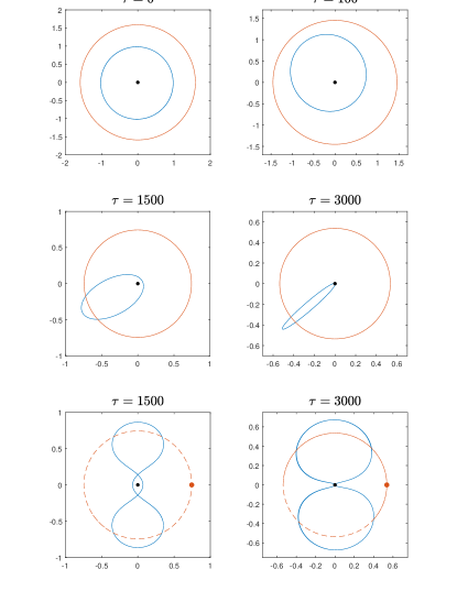
Consider the planar hierarchical restricted three-body problem: a test mass (a star) affected by two dominant masses (a BH binary), co-rotating unperturbed by the test mass on circular orbits around their center of mass, as illustrated in figure 1. Assume that the dominant masses slowly loose their energy, and therefore spiral inwards. The Hamiltonian of this system can be written as
| (1) |
where and are the distances from the dominant masses, , is the rotation angle of , and . We will consider the case in which the test mass starts on a circular orbit of radius at the angular frequency . Note that in equation (1), is replaced by unity. This can be done by using dimensionless time , dimensionless distances and , and dimensionless momenta: and , where . As mentioned above, we will assume that is a slow function of time, i.e. , where . We will also assume that the mass ratio is a small parameter (), as some aspects of our theoretical modeling will break down as . At the most basic level, resonance overlap begins to severely destabilize individual mean motion resonances for large values. Both analytic resonance overlap criteria (Wisdom, 1980) and numerical orbit integrations (Holman & Wiegert, 1999; Mudryk & Wu, 2006) show that when , the 2:1 mean motion resonance becomes unstable, and stars that are temporarily placed in it will quickly escape due to chaotic orbital evolution.

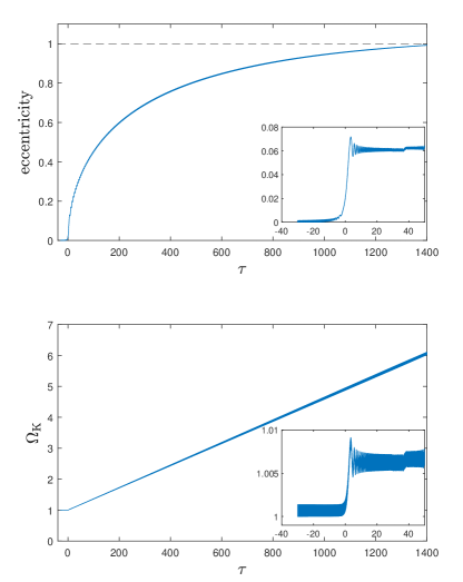
We illustrate the process of resonant capture of the test mass into resonance and continuing autoresonance in this system in numerical examples in figures 2 and 3 for the case of , chirped rotation frequency and constant chirp rate . The resonance passage in this example takes place at and four upper panels in Fig. 2 show the orbits of the three masses at different times (the slow time is used in the figures). One observes that the eccentricity of the test mass increases continuously reaching near unity at . The lower two panels in Fig. 2 show the trajectories in the co-rotating plane and illustrate that the test mass closely approaches, but never collides with the secondary mass . Additional simulation results are presented in Fig. 3 for larger showing the eccentricity of the test mass and its Keplerian frequency as functions of the slow time . One can see that again the eccentricity of the mass approaches unity, while the Keplerian frequency closely follows in time constituting the continuing autoresonance in the system. Nevertheless, for even larger chirp rate, (inner panels in Fig. 3) the resonance is destroyed close to and the eccentricity remains small. We find that this loss of autoresonance in our system takes place if exceeds some threshold value scaling as and discuss this phenomenon next.
3 Capture into Autoresonance and the Threshold Phenomenon
In analysing our system, we expand and in equation (1) to first order in and rewrite , where
| (2) |
is the unperturbed Hamiltonian and
| (3) |
with and . The following analysis is similar to that in Friedland (2001) for the problem of formation of Plutinos in the early stages of evolution of the solar system, but in contrast to Plutinos we consider the case of inner resonances, i.e. .
We can rewrite equation (3) as an expansion in harmonics of :
| (4) |
where are expressed in terms of the Laplace’s coefficients (Tremaine, 2023):
| (5) |
The next step is to transform the problem to the action-angle (AA) variables of the unperturbed Hamiltonian (see Appendix A for details): , and to use single resonance approximation (Chirikov, 1979) (see Appendix C). This yields the approximate resonant Hamiltonian for the resonance of the form
| (6) |
where
| (7) |
and is the resonant angle mismatch ( was subtracted for convenience as explained below). The unperturbed Hamiltonian yields the Kepler frequency of the unperturbed test mass
| (8) |
Note that the vicinity of resonance means that
| (9) |
i.e., in resonance, the mismatch angle is a slow variable.
In this section we will focus on the initial stage of the resonant capture, i.e. the case of small eccentricities (small . As shown in Appendix B for this case, the resonant perturbing potential assumes the following approximate form
| (10) |
where for the first three resonances , , and . Then, equation (6) yields the following evolution equations
| (11) | |||||
| (12) | |||||
| (13) |
The first two of these equations give the conservation law (using the initial values , and )
| (14) |
Therefore, the whole system can be described by and only.
We will focus on passage through resonance at , i.e., write , where is the local driving frequency chirp rate at the. Furthermore, assuming small , one can use Eqs. (8) and (14) to approximate . Then equation (13) becomes
| (15) |
and at negative times prior passage through resonance when is sufficiently small,
| (16) |
It is the singularity at in the last term in this equation which yields efficient phase-locking in the system near the fixed point , at negative times. After the passage through resonance, automatically adjusts in time to stay in the continuing resonance Friedland (2001), while remains small and oscillates around 0 (this was the reason for subtracting in the definition of above).
Equations (11) and (15) comprise a standard set describing the autoresonance phenomenon (Friedland, 2009), which can be conveniently simplified by defining , the slow time , and . With these definitions, Eqs. (11) and (15) yield a single parameter system
| (17) | |||||
| (18) |
This system can be rewritten as a single complex nonlinear Schrodinger-type equation by defining :
| (19) |
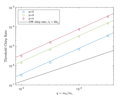
One finds that by starting with at negative times (Friedland, 2009), this equation yields a sharp threshold phenomena: above a critical value , the system is excited to large amplitudes at positive times, while remains small. In contrast, below this threshold, remains small while diverges. Therefore, the test mass in our problem is captured into autoresonance if , or
| (20) |
where , , and . The transition from above to below the threshold is seen in the example in figure 3. One also observes a good agreement between the theoretical and numerical thresholds for different and as illustrated in figure 4.
Since we consider chirp rates caused by gravitational waves, we have (Peters, 1964)
| (21) |
where the factor was added to make dimensionless. By equating Eqs. (20) and (21), one gets the condition for capture into resonance
| (22) |
where is the gravitational radius of . When the capture into resonance occurs, . Therefore, after some algebra one gets
| (23) |
which means that the capture into resonance is almost always guaranteed, as the right hand side of this inequality is always , and realistic IMBH-SMBH inspirals begin with .
Note that as the phase locking (autoresonance) in the system continues, the resulting growth of and the decrease of yield a continuing growth of the orbital eccentricity
| (24) |
Most importantly, this phase-locking and the growth of the eccentricity towards continue beyond the small regime, as will be shown in the next section.
4 Developed Autoresonance Stage and Stability
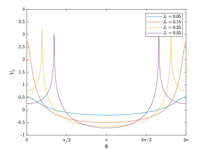
The analysis of the developed autoresonance stage proceeds from the extension of the resonant potential in equation (6) from equation (10) for small to larger values of (larger eccentricities). This generalization is developed in Appendix C using action-angle variables. Unfortunately, doesn’t have a simple analytic form for large , but can be found numerically. Figure 5 shows this perturbing potential for and several values of . The potential still has its minimum at , but a more complex form. In particular, one observes two sharp spikes, starting at . We find that these peaks appear as the orbits of the test mass and the secondary BH cross. The value of for the first such crossing can be found by equating the radius of the outer black hole in autoresonance
where , to the apoapsis distance of the test mass, given by
| (25) |
where is the eccentricity (see Eq. (24)). This comparison and use of the conservation law (14) (the same as for small eccentricities, see below) yields at the crossing of the trajectories
| (26) |
Now, similar to the small case, we write the equations of motion:
| (27) | |||||
| (28) | |||||
| (29) |
yielding the same conservation law
| (30) |
Assuming that following the initial phase-locking stage, the system stays at small values of mismatch , we expand the perturbing potential to second order in , i.e., write
| (31) |
which after substitution into Eqs. (27) and (29), yields
| (32) | |||||
| (33) |
At this stage, we neglect the last term in equation (33). The reason for this approximation will be explained at the end of this section. We seek solutions of the resulting system in the form and where and are small and rapidly oscillating components, while and are slow monotonic averages, which do not vary significantly during a single oscillation of and . By separating the oscillating and monotonic parts in Eqs. (32), (33), we get
| (34) | |||||
| (35) |
and
| (36) | |||||
| (37) |
The analysis of these systems proceeds from Eqs. (36) and (37). We differentiate equation (37) and substitute equation (36) to get
| (38) |
The approximate solution of this equation is obtained by neglecting the LHS, yielding
| (39) |
The smallness and slowness of this solution is guaranteed if which is assumed in the following. Now we can also neglect the LHS in (37) to write
| (40) |
which constitutes the continuing resonance (autoresonance) condition. Finally, we proceed to the oscillating components and of the solution described by (34) and (35). We observe that this is a linear oscillatory Hamiltonian system governed by Hamiltonian
| (41) |
where the slow time dependence enters via coefficients involving . For a frozen slow time the trajectory of this system in phase space is an ellipse
| (42) |
where
| (43) |
Because of the slow time dependence of the parameters and we can use the adiabatic theory (Landau & Lifshitz, 1969) yielding the adiabatic invariant – the action – , where is the area of the ellipse. Thus,
| (44) |
where
| (45) |
is the frequency of the (autoresonant) oscillations. One can write , where and are the amplitudes of oscillations of and respectively. Therefore, given the adiabatic invariant (by initial conditions), we find the time evolution of the amplitudes:
| (46) |
and . Note that both and remain small for sufficiently small , meaning that the stability of the autoresonant system is guaranteed. Finally, we write the adiabaticity condition in our problem
| (47) |
Here equation (40) yields , while . Therefore, condition guaranties the adiabaticity. Note that this is the same condition used above when studying the evolution of the slow system (36) and (37). Finally, note that the RHS in equation (33) evolves as i.e. scales as , which justifies our neglect of term in the right hand side of equation (33) at the beginning of our analysis.
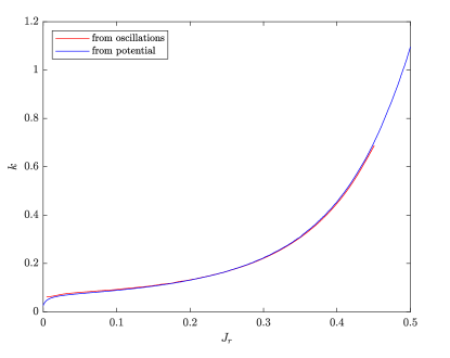
For testing this theory we performed full numerical simulations to find the autoresonant oscillations frequency, which on using equation (45), yields . The latter can be compared with the values obtained from the expansion of the perturbing potential in . This comparison is presented in Fig. 6 showing a good agreement.
.
Lastly, note that the eccentricity of the test mass’ orbit approaches 1 as and the test mass approaches the vicinity of the SMBH. In this case, from equation (30), and from equation (8), we have . Then, using the resonance condition (9), we find the limiting driving frequency for reaching the vicinity of the SMBH.
5 Astrophysical Implications
The theory developed in prior sections will be most applicable to dynamically cold disks of stars surrounding a SMBH in a galactic nucleus. As mentioned in Sec. 1, such disks arise naturally in the aftermath of AGN episodes: after the gas is accreted or blown away, young, thin disks of stars on quasi-circular orbits are left behind (Levin & Beloborodov, 2003), and may also naturally host IMBHs (Goodman & Tan, 2004a).
While analytic and semi-analytic models exist to estimate the surface number density of stars formed by Toomre instability in AGN disks (Thompson et al., 2005; Gilbaum & Stone, 2022), these distributions may be sculpted by stellar migration within the disk due to hydrodynamic interactions, which carries significant uncertainties (Grishin et al., 2023). may be further modified by capture (due to hydrodynamic drag) of stars from the pre-existing nuclear star cluster, from initially inclined orbits (Syer et al., 1991). Despite these substantial uncertainties, we can build an explicit model for by assuming (i) a Shakura-Sunyaev structure (Shakura & Sunyaev, 1973) for the inner regions of the AGN disk; (ii) a steady-state inward flux of migrating stars, , which is a fixed fraction of the inward gas accretion rate (i.e. ); (iii) migration rates that are a combination of “Type I” torques (Goldreich & Tremaine, 1980) and GW torques (Peters, 1964), producing a total (specific) migratory torque , where
| (48) |
Here we consider the migration of stars with individual masses and mass ratios with respect to the central MBH. The Type I torques produced by the hydrodynamic response of the gas disk to stellar gravity depend on the disk’s gas surface mass density and aspect ratio , hydrodynamic variables for the Shakura-Sunyaev disk model that we define in Appendix D. We assume in this section that the orbital frequency is Keplerian, . The dimensionless prefactor can be approximated as (Paardekooper et al., 2011):
| (49) |
where and are the local power-law slopes of the gas temperature and surface density profiles, respectively.
Likewise, the specific migratory torque
| (50) |
results in a GW inspiral time
| (51) |
for circular orbits. We only specify torques (and not dissipation rates) because orbital migration quickly damps out eccentricity, producing quasi-circular inspirals.
Our three underlying assumptions listed above become less accurate as one moves to large radii , where the gas disk structure will be heavily modified by Toomre instability and feedback (Thompson et al., 2005; Gilbaum & Stone, 2022), where stellar fluxes are unlikely to be in a steady state (Gilbaum & Stone, 2022), and where additional types of migratory torques may become relevant (Grishin et al., 2023). However, as we shall see, it is the smaller radii that produce the most directly observable signatures of resonance capture, in the form of elevated TDE rates, motivating these assumptions.
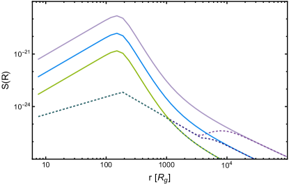
In Fig. 7, we plot example distributions as functions of cylindrical radius in a thin stellar disk. We show two families of such distributions: first, a naive one, in which a constant inwards flux of stars is computed in the continuum limit and determined by the steady state condition:
| (52) |
where . These naive distributions are strongly peaked at small radii, near the radius where radiation pressure gives way to gas pressure in the progenitor gas disk.
After the gas dissipates, the “left-behind” disk of stars will cease its hydrodynamic migration, but will continue to evolve due to (i) GW inspiral, and (ii) direct physical collisions between stars, which rapidly deplete the disk population on scales . As star-star collision times are far shorter than GW inspiral times for distant IMBHs, we assume that shortly after the AGN episode ends, stars at semimajor axis will be radially separated by roughly their own Hill sphere distance, . An alternative possibility is that the stars may assemble into a resonant chain (Secunda et al., 2019), which could have a higher or lower surface density depending on the value of . Under our assumption of Hill sphere separations, we wind up with a 2D surface number density
| (53) |
In practice, we take as a realistic stellar disk surface density.
If an IMBH has formed at larger regions in the AGN disk (Goodman & Tan, 2004b; McKernan et al., 2012b; Secunda et al., 2020), its inward migration during the AGN episode may be heavily slowed by opening a gap (Kanagawa et al., 2018), allowing it to survive until the gas has dissipated. Its subsequent GW-driven inspiral will capture populations of disk stars into autoresonance; as we have shown above, the capture probability will be for the resonance and initially circular orbits. The growth of stellar eccentricity following resonant capture will lead the individual stars to tidally disrupt, at a rate set predictably by Eq. (51). We plot the resulting TDE rate in Fig. 9, showing how different models produce very high TDE rates in the decades and centuries prior to merger, but when a more realistic stellar profile is used, we obtain TDE rates in the final decade before the SMBH merger.
We note that even the eroded stellar densities of may overestimate the true population of stars at small radii if a long enough period of time has passed, so that the stars themselves undergo a GW-driven inspiral (possibly terminating their lives as some type of quasi-periodic eruption, e.g. Metzger et al. 2022; Linial & Sari 2023). For a post-AGN stellar disk of age , we compute the critical semimajor axis that an object of mass needs to survive:
| (54) |
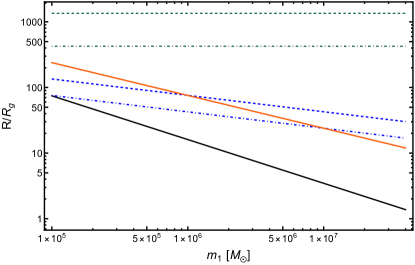
By setting and , we compute , the semimajor axis of the IMBH one decade prior to merger. We then find the system age that gives ; this critical system age . Finally, we use this system age to compute , the maximum initial semimajor axis of the IMBH at the end of the AGN episode; IMBHs that begin at larger radii will not have enough time to migrate into the 2:1 resonance before the left-behind stars are depleted by GW inspiral. The simple result of this is that
| (55) |
This is a sufficiently large radius to be a plausible site for either IMBH formation (in e.g. a migration trap) or for the IMBH to have stalled hydrodynamically due to gap opening (Grishin et al., 2023). The relevant radial scales are shown in Fig. 8 for a red dwarf. We see that there is little parameter space for autoresonant capture when , but the process is feasible for supermassive MBH primaries.
Although the model presented above gives us a simple way to estimate surface densities of disk stars left behind after a major AGN episode, and the TDE rates that result from resonant capture by an inward migrating IMBH, it contains a number of significant assumptions, which we summarize here:
-
•
Migration of stars (and compact objects) through the gas disk is due purely to Type I hydrodynamic torques and GW dissipation. This model neglects the Type II (Kanagawa et al., 2018) migration regime (which is unlikely to be triggered in much of the AGN parameter space; Gilbaum & Stone 2022) and the substantially more uncertain thermal torques. Importantly, we assume that no migration traps (i.e. regions where exist in the disk, as these would make a steady-state stellar inflow solution of our type impossible to achieve. The existence of migration traps in AGN disks has been predicted in the past (Bellovary et al., 2016), but the most recent calibrations of Type I torques (Jiménez & Masset, 2017) are incompatible with such traps on the small scales relevant for us (Grishin et al., 2023).
-
•
Stars move through the disk on quasi-circular, prograde orbits. This is likely a good assumption for stars that form in situ (Stone et al., 2017), or those that capture into the disk on prograde orbits (and circularize/align). However, we neglect stars that capture on retrograde orbits, as (i) these will not possess orbital resonances with the outer MBH binary, and (ii) they may be quickly destroyed due to eccentricity excitation from gas dynamical friction (Secunda et al., 2021).
-
•
A steady state solution is established, where the flux of stars through the inner disk, , equals some quasi-steady rate of star formation and capture in the outer disk. Such a steady state could be complicated by vigorous accretion feedback from embedded compact objects (Chen et al., 2023), but that is beyond the scope of this work.
-
•
The gas dissipates fairly quickly throughout the entire AGN disk, so that the steady-state inflow solution “freezes in” as the AGN episode ends. To the extent that this assumption is violated, it will cause deviations from our profiles in regions with the shortest migration times ; these are generally regions with smaller densities and (as we shall see) lower contributions to the TDE rate.
In summary, the final few decades of SMBH-IMBH inspiral through the disk of stars left behind after an AGN episode will see TDE rates rise several orders of magnitude above their values in normal galactic nuclei (where ; Stone & Metzger 2016; Yao et al. 2023). These rates are high enough that a significant percentage of LISA-band mergers (tens of percent) from such systems will see an individual TDE flare in the final decade before LISA detection. This type of electromagnetic counterpart opens the door to host galaxy identification, the implications of which we will discuss in the final section.
6 Conclusions
We have studied the resonant dynamics of stars in the vicinity of a hierarchical massive black hole binary and discussed the resulting TDE rate into the central SMBH in the binary. Our fiducial calculations were motivated by disks of stars that form from Toomre instability in AGN episodes (Levin & Beloborodov, 2003; Levin, 2007; Gilbaum & Stone, 2022), as well as IMBHs that may also arise (Goodman & Tan, 2004b; McKernan et al., 2012a) in these disks. The simple geometry of this scenario allowed us to use the planar restricted three-body limit to analyze the capture of stars into resonance as the MBH binary decays from gravitational wave losses. For stars that (i) are well interior to the binary orbit and (ii) are initially on nearly circular orbits, capture into the 2:1 resonance is guaranteed if the chirp rate of the Keplerian frequency of the secondary BH is below a threshold that is always satisfied for astrophysical inspirals. After the capture into resonance, the stars stay in resonance continuously and increase their orbital eccentricity towards unity (Yu & Tremaine, 2001b). The drop in the test particle’s pericenter distance eventually leads to a TDE, provoking a bright electromagnetic outburst accompanying the MBH binary inspiral (Seto & Muto, 2010, 2011). This precursor TDE can serve as an electromagnetic counterpart distinct from postcursor TDEs which may be expected due to GW recoil after the MBH merger (Stone & Loeb, 2011; Akiba & Madigan, 2021)
This autoresonant process is similar to that in the formation of Plutinos in the Kuiper Belt in early evolution of the Solar system (Friedland, 2001). However, in contrast to the Plutinos, which capture into outer mean motion resonances, the capture of stars into autoresonance by MBH binaries involves inner resonances (Yu & Tremaine, 2001b). The TDEs produced by autoresonance have a very different dynamical origin than the classical “loss cone” picture, in which weak, diffusive star-star scatterings cause a slow random walk in stellar orbits up to high eccentricity. Since this novel channel of TDEs occurs on the time scale of the MBH inspiral and involves a large number of stars in autoresonance, we predict much higher rates of disruptions than the classical channel. The peak rates we find in the final decade of an SMBH-IMBH inspiral can be as high as , far greater than the predicted by loss cone theory (Stone & Metzger, 2016) or the even lower found by current optical surveys of TDEs. The elevated rate suggests that some galactic nuclei may exhibit multiple TDEs, creating a possible tracer of the binary MBH population. This channel will also give rise to multi-messenger observations: an electromagnetic flare from the TDEs that accompanies or precedes the mHz gravitational wave signal from an inspiraling SMBH-IMBH binary. If such a multimessenger signal could be detected, it would be of extreme astrophysical value: LISA sky error regions are too large to permit host galaxy localization, but if the host can be identified, the luminosity distance measurement from GWs could be combined with an electromagnetic redshift to enable “standard siren” cosmological measurements (Schutz, 1986).
In our analysis we have made several simplifying assumptions. The first and most obvious one is the planarity of the problem – we have studied a system in which both the MBHs, and the test stars, all orbit in a single plane. While this assumption is well-motivated for the “left-behind” stellar disks following AGN episodes, many other MBH binaries form in quasi-spherical nuclear star clusters (Milosavljević & Merritt, 2001; Merritt & Milosavljević, 2005). In a quasi-spherical system, generic stellar orbits will initially be both misaligned and eccentric, a more complicated problem that can be explored by numerical integration (Namouni & Morais, 2015). A second assumption concerning system parameters is that of an extreme mass ratio () between the primary SMBH and the secondary IMBH. While, again, this is reasonably well motivated for IMBHs that form in AGN disks, such extreme mass ratios will be uncommon for MBH binaries produced by galaxy mergers, as the dynamical friction time for a very low-mass satellite can exceed the age of the Universe (Taffoni et al., 2003). As increases, non-linear effects may destabilize autoresonant capture, and it is likely that capture probabilities will need to be assessed by numerical simulations.
Other assumptions we have made concern the underlying physics rather than the parameters of the problem. For example, we treat gravity as being purely Newtonian for the test particle (though of course it is relativistic radiation reaction that powers the MBH inspiral). The leading order impact of general relativity is to induce apsidal precession, which may affect the stability of resonances as eccentricity increases. We have also considered single star dynamics only, disregarding star-star scattering events. Stellar scattering may reduce TDE rates by knocking stars out of autoresonance; on the other hand, if relativistic apsidal precession causes a high-eccentricity exit from resonance, a very small amount of star-star scattering may cause these stars to random walk into a TDE. Finally, we have neglected the population of higher order resonances (e.g. 3:1 or 4:1) that stars will encounter before the 2:1 resonance. However, capture into these resonances at mass ratios studied here is probabilistic rather than deterministic, so we expect that an fraction of disk stars will pass through higher order resonances without a major impact on their orbit before encountering the 2:1 resonance.
In summary, autoresonant capture of stars by inspiraling MBH binaries is capable of producing bursts of TDEs during the final stages of MBH mergers. While this first investigation shows that these TDE bursts have potential as electromagnetic counterparts to LISA-band signals, their overall relevance must be quantified by further analytic and numerical studies relaxing some of the assumptions listed above.
References
- Akiba & Madigan (2021) Akiba T., Madigan A.-M., 2021, ApJ, 921, L12
- Amaro-Seoane (2018) Amaro-Seoane P., 2018, Living Reviews in Relativity, 21, 4
- Amaro-Seoane et al. (2022) Amaro-Seoane P., et al., 2022, arXiv e-prints, p. arXiv:2203.06016
- Arcavi et al. (2014) Arcavi I., et al., 2014, ApJ, 793, 38
- Babak et al. (2017) Babak S., et al., 2017, Phys. Rev. D, 95, 103012
- Bar-Or & Alexander (2016) Bar-Or B., Alexander T., 2016, ApJ, 820, 129
- Bartko et al. (2010) Bartko H., et al., 2010, ApJ, 708, 834
- Begelman et al. (1980) Begelman M. C., Blandford R. D., Rees M. J., 1980, Nature, 287, 307
- Bellovary et al. (2016) Bellovary J. M., Mac Low M.-M., McKernan B., Ford K. E. S., 2016, ApJ, 819, L17
- Broggi et al. (2022) Broggi L., Bortolas E., Bonetti M., Sesana A., Dotti M., 2022, MNRAS, 514, 3270
- Chen et al. (2023) Chen K., Ren J., Dai Z.-G., 2023, ApJ, 948, 136
- Chirikov (1979) Chirikov B. V., 1979, Phys. Rep., 52, 275
- Cohn & Kulsrud (1978) Cohn H., Kulsrud R. M., 1978, ApJ, 226, 1087
- Cuadra et al. (2009) Cuadra J., Armitage P. J., Alexander R. D., Begelman M. C., 2009, MNRAS, 393, 1423
- Frank & Rees (1976) Frank J., Rees M. J., 1976, MNRAS, 176, 633
- Friedland (2001) Friedland L., 2001, ApJ, 547, L75
- Friedland (2009) Friedland L., 2009, Scholarpedia, 4, 5473
- Gezari et al. (2006) Gezari S., et al., 2006, ApJ, 653, L25
- Gezari et al. (2008) Gezari S., et al., 2008, ApJ, 676, 944
- Gilbaum & Stone (2022) Gilbaum S., Stone N. C., 2022, ApJ, 928, 191
- Goldreich & Tremaine (1980) Goldreich P., Tremaine S., 1980, ApJ, 241, 425
- Goodman & Tan (2004a) Goodman J., Tan J. C., 2004a, ApJ, 608, 108
- Goodman & Tan (2004b) Goodman J., Tan J. C., 2004b, ApJ, 608, 108
- Gould & Rix (2000) Gould A., Rix H.-W., 2000, ApJ, 532, L29
- Greene et al. (2020) Greene J. E., Strader J., Ho L. C., 2020, ARA&A, 58, 257
- Grishin et al. (2023) Grishin E., Gilbaum S., Stone N. C., 2023, arXiv e-prints, p. arXiv:2307.07546
- Hayasaki et al. (2007) Hayasaki K., Mineshige S., Sudou H., 2007, PASJ, 59, 427
- Hills (1975) Hills J. G., 1975, Nature, 254, 295
- Hoffman & Loeb (2007) Hoffman L., Loeb A., 2007, MNRAS, 377, 957
- Holman & Wiegert (1999) Holman M. J., Wiegert P. A., 1999, AJ, 117, 621
- Hopman & Alexander (2005) Hopman C., Alexander T., 2005, ApJ, 629, 362
- Hung et al. (2017) Hung T., et al., 2017, ApJ, 842, 29
- Inayoshi et al. (2020) Inayoshi K., Visbal E., Haiman Z., 2020, ARA&A, 58, 27
- Jiménez & Masset (2017) Jiménez M. A., Masset F. S., 2017, MNRAS, 471, 4917
- Kanagawa et al. (2018) Kanagawa K. D., Tanaka H., Szuszkiewicz E., 2018, ApJ, 861, 140
- Komossa & Bade (1999) Komossa S., Bade N., 1999, A&A, 343, 775
- Komossa & Greiner (1999) Komossa S., Greiner J., 1999, A&A, 349, L45
- Landau & Lifshitz (1969) Landau L. D., Lifshitz E. M., 1969, Mechanics
- Levin (2007) Levin Y., 2007, MNRAS, 374, 515
- Levin & Beloborodov (2003) Levin Y., Beloborodov A. M., 2003, ApJ, 590, L33
- Linial & Sari (2023) Linial I., Sari R., 2023, ApJ, 945, 86
- Lodato et al. (2009) Lodato G., Nayakshin S., King A. R., Pringle J. E., 2009, MNRAS, 398, 1392
- Lu et al. (2013) Lu J. R., Do T., Ghez A. M., Morris M. R., Yelda S., Matthews K., 2013, ApJ, 764, 155
- Luo et al. (2016) Luo J., et al., 2016, Classical and Quantum Gravity, 33, 035010
- McKernan et al. (2012a) McKernan B., Ford K. E. S., Lyra W., Perets H. B., 2012a, MNRAS, 425, 460
- McKernan et al. (2012b) McKernan B., Ford K. E. S., Lyra W., Perets H. B., 2012b, MNRAS, 425, 460
- Merritt & Milosavljević (2005) Merritt D., Milosavljević M., 2005, Living Reviews in Relativity, 8, 8
- Merritt & Poon (2004) Merritt D., Poon M. Y., 2004, ApJ, 606, 788
- Metzger et al. (2022) Metzger B. D., Stone N. C., Gilbaum S., 2022, ApJ, 926, 101
- Miller et al. (2005) Miller M. C., Freitag M., Hamilton D. P., Lauburg V. M., 2005, ApJ, 631, L117
- Milosavljević & Merritt (2001) Milosavljević M., Merritt D., 2001, ApJ, 563, 34
- Milosavljević et al. (2006) Milosavljević M., Merritt D., Ho L. C., 2006, ApJ, 652, 120
- Mockler et al. (2019) Mockler B., Guillochon J., Ramirez-Ruiz E., 2019, ApJ, 872, 151
- Mudryk & Wu (2006) Mudryk L. R., Wu Y., 2006, ApJ, 639, 423
- Namouni & Morais (2015) Namouni F., Morais M. H. M., 2015, MNRAS, 446, 1998
- Nayakshin et al. (2007) Nayakshin S., Cuadra J., Springel V., 2007, MNRAS, 379, 21
- Neumayer et al. (2020) Neumayer N., Seth A., Böker T., 2020, A&ARv, 28, 4
- Paardekooper et al. (2011) Paardekooper S. J., Baruteau C., Kley W., 2011, MNRAS, 410, 293
- Pan & Yang (2021) Pan Z., Yang H., 2021, Phys. Rev. D, 103, 103018
- Paumard et al. (2006) Paumard T., et al., 2006, ApJ, 643, 1011
- Peng & Chen (2023) Peng P., Chen X., 2023, ApJ, 950, 3
- Peters (1964) Peters P. C., 1964, Physical Review, 136, 1224
- Quinlan (1996) Quinlan G. D., 1996, New Astron., 1, 35
- Qunbar & Stone (2023) Qunbar I., Stone N. C., 2023, arXiv e-prints, p. arXiv:2304.13062
- Rees (1988) Rees M. J., 1988, Nature, 333, 523
- Reusch et al. (2022) Reusch S., et al., 2022, Phys. Rev. Lett., 128, 221101
- Ruan et al. (2020) Ruan W.-H., Guo Z.-K., Cai R.-G., Zhang Y.-Z., 2020, International Journal of Modern Physics A, 35, 2050075
- Ryan (1995) Ryan F. D., 1995, Phys. Rev. D, 52, 5707
- Ryu et al. (2018) Ryu T., Perna R., Haiman Z., Ostriker J. P., Stone N. C., 2018, MNRAS, 473, 3410
- Ryu et al. (2020) Ryu T., Krolik J., Piran T., 2020, ApJ, 904, 73
- Sayeb et al. (2024) Sayeb M., Blecha L., Kelley L. Z., 2024, MNRAS, 527, 7424
- Schutz (1986) Schutz B. F., 1986, Nature, 323, 310
- Secunda et al. (2019) Secunda A., Bellovary J., Mac Low M.-M., Ford K. E. S., McKernan B., Leigh N. W. C., Lyra W., Sándor Z., 2019, ApJ, 878, 85
- Secunda et al. (2020) Secunda A., et al., 2020, ApJ, 903, 133
- Secunda et al. (2021) Secunda A., Hernandez B., Goodman J., Leigh N. W. C., McKernan B., Ford K. E. S., Adorno J. I., 2021, ApJ, 908, L27
- Seto & Muto (2010) Seto N., Muto T., 2010, Phys. Rev. D, 81, 103004
- Seto & Muto (2011) Seto N., Muto T., 2011, MNRAS, 415, 3824
- Shakura & Sunyaev (1973) Shakura N. I., Sunyaev R. A., 1973, A&A, 24, 337
- Sigurdsson & Rees (1997) Sigurdsson S., Rees M. J., 1997, MNRAS, 284, 318
- Sirko & Goodman (2003) Sirko E., Goodman J., 2003, MNRAS, 341, 501
- Stein et al. (2021) Stein R., et al., 2021, Nature Astronomy, 5, 510
- Stone & Loeb (2011) Stone N., Loeb A., 2011, MNRAS, 412, 75
- Stone & Metzger (2016) Stone N. C., Metzger B. D., 2016, MNRAS, 455, 859
- Stone et al. (2017) Stone N. C., Küpper A. H. W., Ostriker J. P., 2017, MNRAS, 467, 4180
- Syer et al. (1991) Syer D., Clarke C. J., Rees M. J., 1991, MNRAS, 250, 505
- Taffoni et al. (2003) Taffoni G., Mayer L., Colpi M., Governato F., 2003, MNRAS, 341, 434
- Thompson et al. (2005) Thompson T. A., Quataert E., Murray N., 2005, ApJ, 630, 167
- Toomre (1964) Toomre A., 1964, ApJ, 139, 1217
- Tremaine (2023) Tremaine S., 2023, Dynamics of Planetary Systems
- Vasiliev et al. (2015) Vasiliev E., Antonini F., Merritt D., 2015, ApJ, 810, 49
- Volonteri (2010) Volonteri M., 2010, A&ARv, 18, 279
- Wang & Merritt (2004) Wang J., Merritt D., 2004, ApJ, 600, 149
- Wen et al. (2020) Wen S., Jonker P. G., Stone N. C., Zabludoff A. I., Psaltis D., 2020, ApJ, 897, 80
- Wen et al. (2021) Wen S., Jonker P. G., Stone N. C., Zabludoff A. I., 2021, ApJ, 918, 46
- Wisdom (1980) Wisdom J., 1980, AJ, 85, 1122
- Yao et al. (2023) Yao Y., et al., 2023, ApJ, 955, L6
- Yu & Tremaine (2001a) Yu Q., Tremaine S., 2001a, AJ, 121, 1736
- Yu & Tremaine (2001b) Yu Q., Tremaine S., 2001b, AJ, 121, 1736
- van Velzen (2018) van Velzen S., 2018, ApJ, 852, 72
- van Velzen et al. (2011) van Velzen S., et al., 2011, ApJ, 741, 73
- van Velzen et al. (2019) van Velzen S., Stone N. C., Metzger B. D., Gezari S., Brown T. M., Fruchter A. S., 2019, ApJ, 878, 82
- van Velzen et al. (2021) van Velzen S., et al., 2021, ApJ, 908, 4
Appendix A Action-Angle Variables
Here, for completeness, we summarize the developments yielding the transformation to AA variables in our problem. The planar elliptical Keplerian motion conserves the energy and is periodic in both and , such that in it conserves the angular momentum , while the motion in can be viewed as an oscillation in the one-dimensional potential well . This suggests to define the following azimuthal and radial action variables (Landau & Lifshitz, 1969).
| (56) |
and
| (57) |
The last equation yields relation of the Hamiltonian to the actions
| (58) |
It can be also shown that in the elliptical orbit equation
| (59) |
parameter and eccentricity are simply related to the two actions (Landau & Lifshitz, 1969):
| (60) |
which also yields relations of the major and minor semi axis and to the actions. Finally, we complete the canonical transformation to AA variables by defining the generating function
| (61) |
where . This function gives the required four transformation equations
| (62) | |||||
where
| (63) |
The first two equations in this set are natural connections to the radial and azimuthal momenta, while the last two equations define the canonical angles . Finally, note that since the Hamiltonian does not depend on the angle variables both actions remain constant, while Hamilton equations for the canonical angles are
| (64) |
where – the Keplerian frequency – is defined as
| (65) |
We complete this appendix by discussing the limit of small oscillations around the initially circular orbit of unit radius, i.e., , with angular velocity equal to unity. These are linear oscillations in the potential well mentioned above, and for small action can be expressed as , where the amplitude of the oscillations, as for all linear oscillators, is related to the action via . In addition, for small oscillations, since is the velocity in the potential well,
| (66) |
and thus
| (67) |
This result will be used in Appendix B.
Appendix B Effective potential for Small Eccentricities
In this appendix, we will focus on the case of small eccentricities. In this case, using the single resonance approximation (Chirikov, 1979), we leave a single -th harmonic term in the perturbing potential (4), i.e.
| (68) |
Here we write (see the end of A) , where . Then, by expanding to first order in , we get
| (69) |
where initially, and . Next, we substitute equation (67) into and to get
| (70) |
where and . Here we use equation (66) for , to obtain
| (71) |
Alternatively,
| (72) |
Finally, we leave the only resonant (last) term in this equation, to obtain
| (73) |
where and . The first three coefficients in are , , and .
Appendix C Derivation of the resonant perturbing Potential
Here, we derive the resonant perturbing potential in our problem for arbitrary radial action . We proceed from equation (4) and substitute (62):
| (74) |
This can be rewritten as
| (75) |
where and . The goal is to extract the resonant part in for arbitrary , similar to the development in B for small . We’ll again focus on resonance (), i.e. assume that the system continuously preserves
| (76) |
or equivalently, the phase mismatch remains nearly stationary for all during the autoresonant evolution. Then, we expand and in Fourier series
| (77) |
allowing to write the perturbing potential as
| (78) |
where
| (79) |
Alternatively,
| (80) |
where and . In seeking the resonant contribution, we choose in equation (80) because the coefficients fall rapidly and leave the first cosine term only to get the resonant perturbing potential
| (81) |
The coefficients can be found by using the Fourier series:
| (82) | |||||
| (83) |
yielding
| (84) |
We calculate these coefficients by defining the function
| (85) |
By using Eqs. (85) and (63), to write a system of ODEs
| (86) | |||||
| (87) |
where is given by (65), , by the conservation law derived at equation (30), and is given by the orbit (60) with replaced by
| (88) |
Numerical solution of this system with from to yields coefficients in the resonant perturbing potential . In the case of small eccentricities (see appendix B), we found that coefficients decrease rapidly with allowing to use only single component with in (81). For larger eccentricities, decrease slower and we include additional terms in (81) for convergence.
Appendix D Astrophysical Disk Model
The stellar disks whose component stars are the subject of this paper are ultimately produced as leftovers of AGN episodes, where an axisymmetric disk of gas and plasma orbits a central MBH. Although the precise details of the gas disk turn out not to matter too much for the distribution of stars far after the end of the AGN episode (see §5), we include the relevant equations for the structure of the gas disk here, as they are needed to reach this conclusion.
For simplicity, we treat the AGN disk structure in the standard Shakura-Sunyaev way: as an axisymmetric, geometrically thin disk orbiting in the nearly Newtonian potential of a MBH with mass , with hydrodynamics in a steady state inflow-equilibrium (Shakura & Sunyaev, 1973). The disk is assumed to be sub-Eddington, with no outflows, and the microphysics (opacity, equation of state) are treated in an approximate manner. The disk profile is defined by a 1D surface mass density . At each cylindrical radius there is a disk scale height , a midplane temperature , a pressure , a photon optical depth , a midplane opacity , a midplane gas sound speed , and a midplane 3D mass density . Although such a 1D treatment of hydrodynamics is formally laminar, there is also an effective kinematic viscosity which parametrizes the transport of angular momentum by small-scale turbulent motions. The system of algebraic equations governing the disk structure is
| (89) | ||||
| (90) | ||||
| (91) | ||||
| (92) | ||||
| (93) | ||||
| (94) | ||||
| (95) | ||||
| (96) | ||||
| (97) |
In these equations, we assume nearly Keplerian gas motion at a frequency . The total opacity is the sum of electron scattering opacity and the Kramers parametrization of bound-free opacity, , where we assume that the hydrogen, helium, and metal mass fractions have Solar-like values of , , and , respectively. We note that is the radiation constant, the Stefan-Boltzmann constant, the Boltzmann constant, the gas adiabatic index (which varies between and according to Eq. 92), is the proton mass, and is the mean molecular weight. The dimensionless function arises from assuming zero hydrodynamical stress at the inner boundary , and the dimensionless Shakura-Sunyaev viscosity parameter is set equal to 0.1. These 9 equations are combined numerically into a single equation which is solved numerically by root-finding to yield disk profiles such as , , etc.