Flexible and Efficient Estimation of Causal Effects with Error-Prone Exposures: A Control Variates Approach for Measurement Error

Abstract

Exposure measurement error is a ubiquitous but often overlooked challenge in causal inference with observational data. Existing methods accounting for exposure measurement error largely rely on restrictive parametric assumptions, while emerging data-adaptive estimation approaches allow for less restrictive assumptions but at the cost of flexibility, as they are typically tailored towards rigidly-defined statistical quantities. There remains a critical need for assumption-lean estimation methods that are both flexible and possess desirable theoretical properties across a variety of study designs. In this paper, we introduce a general framework for estimation of causal quantities in the presence of exposure measurement error, adapted from the control variates approach of Yang and Ding (2019). Our method can be implemented in various two-phase sampling study designs, where one obtains gold-standard exposure measurements for a small subset of the full study sample, called the validation data. The control variates framework leverages both the error-prone and error-free exposure measurements by augmenting an initial consistent estimator from the validation data with a variance reduction term formed from the full data. We show that our method inherits double-robustness properties under standard causal assumptions. Simulation studies show that our approach performs favorably compared to leading methods under various two-phase sampling schemes. We illustrate our method with observational electronic health record data on HIV outcomes from the Vanderbilt Comprehensive Care Clinic.

Keywords— Causal inference, Control variates, Doubly-robust, HIV, Measurement error, Validation data

1 Introduction

Measurement error poses a significant challenge in public health applications ranging from environmental health to nutritional epidemiology. Examples include area-level air pollution measurements extrapolated from sensors in fixed locations, self-reported dietary consumption patterns deviating considerably from true consumption patterns, and reported adherence to daily-regimen treatments like pre-exposure prophylaxis, which are often biased. These three scenarios are just a few examples of an overarching problem in observational and experimental studies – the exposure of interest is often difficult and/or expensive to measure correctly. In these scenarios, researchers often resort to using error-prone measurements as proxies of the true exposure. In the context of parametric models, it is well-understood that measurement error in an exposure of interest, if ignored, can lead to severely biased inferences (Carroll et al. 2006).

While a rich literature exists on statistical methods for analyzing error-prone data (Carroll et al. 2006), measurement error methods have only recently been situated within a formal causal inference framework. In the causal inference context, methods are generally designed specifically to address measurement error in either the exposure variable, the outcome variable, or the confounding variables (Valeri 2021). Much of the focus has been on parametric, propensity score-based causal analyses with binary exposures (Braun et al. 2017), though recent work has extended methods to continuous (Josey et al. 2023) and categorical error-prone exposures (Wu et al. 2019). While in this work we focus on exposure measurement error and misclassification, there have been related developments in the causal inference literature for addressing differential measurement error in the outcome variable (Ackerman et al. 2021; Kallus and Mao 2020), as well as measurement error in confounding variables. In particular, measurement error in confounding variables has been extensively studied; Webb-Vargas et al. (2017) consider multiple imputation-based methods, Kyle et al. (2016) extend the simulation extrapolation (SIMEX) method to account for measurement error in time-varying confounders in marginal structural models, and Hong et al. (2017) consider Bayesian approaches to addressing confounder measurement error.

To date, much of the literature at the intersection of causal inference and measurement error has considered methods that rely on parametric models for the measurement error mechanism, the treatment assignment, and the outcome. This trend stems mainly from the long-established measurement error literature, which has primarily focused on bias corrections in parametric models (Wang 2021). In turn, much of the work in causal inference has ostensibly borrowed from developments in the measurement error literature with the focus directed on inference in the context of parametric data-generating processes. While parametric modeling has played a key role in the development of causal methods, the disproportionate number of methods based on parametric modeling in measurement error applications is largely out of step with recent developments in the causal inference literature that emphasize targeting explicitly defined estimands without the reliance on assumption-heavy models.

The causal inference community has recognized this shortcoming, and in recent years encouraging progress has been made towards the development of robust methods that make fewer assumptions about the underlying data generating process in measurement error problems. In particular, recent developments have been spurred by approaches that recast measurement error as a missing data problem, allowing one to implement existing tools and theory to derive improved estimators (Keogh and Bartlett 2021). As an example of the modern robust missing data methods that could be adapted to address measurement error problems, Kennedy (2020) proposed efficient, doubly robust methods for estimating average treatment effects under partially missing exposure information. Their method is readily adaptable to scenarios where error prone observations are treated as missing data. In a similar spirit, but in the context of partially missing outcomes, Kallus and Mao (2020) developed semi-parametric efficient estimators for estimating average treatment effects that can be leveraged in scenarios where the outcome of interest is measured with error. While these methods have attractive theoretical properties, their adoption into applied research has been slow, largely due to a lack of flexibility. By construction these methods highly are specific, meaning that small tweaks to the estimation problem often yield a vastly different estimator. In turn, there is a need for methods that possess the attractive properties typical of doubly-robust estimators, while accommodating numerous study designs and potential sources of bias in a general manner that facilitates their uptake.

Despite the recent progress in methods for causal inference with measurement error, there remains a critical need for methods that are easy to implement in a broad range of measurement error problems and study designs. In this paper, we address these needs by proposing a general framework for estimation of causal quantities in the presence of exposure measurement error through adaptations of the control variates framework developed by Yang and Ding (2019). The control variates framework leverages a subset of validated exposure measurements to identify and correct for biases due to measurement error and to quantify the correlation between the gold-standard and error-prone effect estimates, which is used in combination with the information from the full sample to achieve an estimator with reduced variance. We show that these estimators perform competitively with existing estimators under common two-phase sampling schemes, with capability to account for simultaneous outcome measurement error. Simulation studies show that our method performs similarly to commonly-used methods for addressing measurement error, while additionally possessing the ability to handle study designs for which the current leading approaches are not well-suited. Moreover, our method is straightforward to implement, only requiring small augmentations to existing popular software tools for conducting causal inference research.

The remainder of this paper is structured as follows. In Section 2, we define the problem setting, causal estimands of interest and relevant assumptions. Section 3.1 introduces our proposed control variates method under a simplified scenario where the validation data are randomly sampled through a two-phase sampling scheme. Section 4 presents the results of a simulation study comparing the control variates method to existing popular measurement error correction approaches. In Section 6, we assess the performance of our proposed method in real-world settings by applying it to data from the Vanderbilt Comprehensive Care Clinic (VCCC). Section 5 discusses extensions to the control variates method that address settings where the validation data is not a random subset of the main data. Finally, Section 7 concludes with a discussion of our findings and avenues for future research.

2 Problem Setting

2.1 Data and Notation

Suppose a researcher obtains independent samples $\bm{O}_{i}=(Y_{i},A_{i},A_{i}^{*},\bm{X}_{i},S_{i}),\ i\in\{1,\ldots,n\}$, from a target population of interest. $A_{i}^{*}$ is an error-prone measurement of the true binary exposure indicator $A_{i}$. We assume access to an internal validation sample for which gold-standard measurements of the true exposure $A_{i}$ are available. Selection into the internal validation sample is denoted by the binary variable $S_{i}$, and accordingly $A_{i}$ is observed when $S_{i}=1$ and missing otherwise. $Y_{i}$ denotes the outcome of interest, and $\bm{X}_{i}$ vector of covariates, which are both initially assumed to be measured without error. Throughout, we adopt the Rubin potential outcomes framework (Rubin 1974), letting $Y_{i}(a)$ denote the outcome subject $i$ would have experienced had they received treatment $A_{i}=a,\ a\in\{0,1\}$. Importantly, we define potential outcomes in terms of the true treatment value, not their error-prone measurements.
While the availability of a validation dataset—joint observations of error-prone and error-free measurements of an exposure—may seem relatively uncommon, there are numerous instances of such data structures in applied research. Consider two-phase sampling schemes (Carroll et al. 2006), which are often employed when measurement of key variables is difficult. In these schemes, a large dataset is initially sampled from a target population. Then for a subset of the original sample, gold-standard measurements of the difficult-to-measure variables are obtained. Moreover, this structure is often seen in studies where subjects with error-prone measurements from a main dataset can be linked to gold-standard measurements from an external source. One common example occurs within medical claims data, when investigators can link patients with error-prone medical claims data to external data sources with more detailed information. For numerous examples of studies that have made use of validation data to address measurement error, see Web Appendix Table 3 in the Supplementary Materials.

We assume that the true and error-prone exposure measurements are related by a particular variant of a classical, differential measurement error model. Such models 1) assume that the true exposure value is a direct cause of the error-prone measurement and 2) allow for possible correlation between the severity of the measurement errors and the observed outcomes $Y$. Critically, and contrary to much of the measurement error literature, we make no a priori assumptions on the functional form of the measurement error mechanism that relates $A$ to $A^{*}$. As will be discussed in Section 3.1, our proposed approach circumvents the modeling of this process by leveraging the correlation between the true and error-prone variables.

2.2 Causal Estimand

While our proposed methodology is applicable to general functions of counterfactual means, for clarity we fix our interests in estimating the target average treatment effect (TATE):

$$\tau_{\text{TATE}}\overset{\text{def}}{=}\mathbb{E}[Y(1)-Y(0)],$$

the average treatment effect of the exposure on the outcome within the population from which the main data is sampled. The distinction placed on the target population is necessary because, even if the full sample is a random sample of the target population, it may not be the case that the validation sample is. Recall that $A_{i}$ is partially unobserved in the main study data. Since we wish to avoid assumptions about the structure of the measurement error, we begin by discussing the conditions needed to identify $\tau_{\text{TATE}}$ using only the validation data, where $A_{i}$ is observed.

Assumption 1 (SUTVA)

$Y_{i}=Y_{i}(A_{i})$ for all study units. Further, the potential outcomes of any fixed unit are not a function of the treatment status of any other unit: $Y_{i}(a)\perp\!\!\!\perp A_{j}$ for all $i\neq j$.

Assumption 2 (Positivity)

$\mathbb{P}(A=1|\bm{X}=\bm{x})>0$ for all $\bm{x}$ with positive support.

Assumption 3 (Unconfoundedness)

$(Y(1),Y(0))\perp\!\!\!\perp A|\bm{X}$.

When Assumptions 2-3 additionally hold for all subjects with $S=1$, the treatment effect corresponding to the population of the validation data distribution, $\tau_{\text{val}}\overset{\text{def}}{=}\mathbb{E}(Y(1)-Y(0)|S=1)$, can be identified as

$$\tau_{\text{val}}=\mathbb{E}_{\bm{X}|S=1}[\mathbb{E}(Y|\bm{X},S=1,A=1)-\mathbb{E}(Y|\bm{X},S=1,A=0)].$$ (1)

The manner in which the validation data is obtained dictates whether $\tau_{\text{val}}=\tau_{\text{TATE}}$. In particular, one common study design is to obtain a simple random sample from the main dataset to validate. Such study designs are consistent with an assumption that validation data is available completely at random:

Assumption 4 (Validation completely at random)

$(Y(1),Y(0),\bm{X},A,A^{*})\perp\!\!\!\perp S$.

Under Assumption 4, we have $\tau_{\text{TATE}}=\tau_{\text{val}}$, implying that when Assumptions 1-3 also hold, one can consistently estimate $\tau_{\text{TATE}}$ using only observations from the validation data. While often employed in practice simple random validation samples are not always feasible. Instead, it is often the case that the availability of validation data is a function of observed, and potentially unobserved, baseline factors. To accommodate such settings, we consider scenarios where the following assumptions hold in place of Assumption 4:

Assumption 5.a (Validation selection exchangeability)

$Y\perp\!\!\!\perp S|\bm{X},A$.

Assumption 5.b (Positivity of validation selection)

$0<P(S=1|\bm{X}=\bm{x})<1$ for all $\bm{x}$ with positive support.

(a) Selection into the validation data occurs completely at random.

(b) Selection into the validation data is random conditional on baseline covariates.

Figure 1: Comparison of two scenarios involving classical, possibly differential measurement error. Dashed arrows indicate causal dependencies that can be present or absent.

hese two sets of independence assumptions are expressed through the DAGs in Figure 1(a) and 1(b). Note that under either set of independence assumptions, $\tau_{\text{TATE}}$ can be identified by the G-computation functional

$$\tau_{\text{TATE}}=\mathbb{E}_{\bm{X}}[\mathbb{E}(Y|\bm{X},S=1,A=1)-\mathbb{E}(Y|\bm{X},S=1,A=0)].$$ (2)

Assumption 5.a guarantees that the conditional average treatment effect (CATE) function $\mathbb{E}(Y|\bm{X},A=a)=\mathbb{E}(Y|\bm{X},A=a,S=1)$, where the right-hand side is identifiable. One can then identify $\tau_{\text{TATE}}$ by computing a weighted-average of the estimated CATEs according to the distribution of the target population.

3 Methods

3.1 General Framework

Originally developed by Yang and Ding (2019) to address situations with unmeasured confounding in observational studies, the approach later termed the control variates method in Guo et al. (2021) borrows variance reduction tools from the Monte Carlo sampling literature (Rubinstein and Marcus 1985) and is applicable to scenarios where one has access to numerous sources of data, yet the causal quantity of interest is only identifiable in a subset of those sources. We primarily focus on the setting where there are two sources, the validation data and the main data. While previous applications have used the control variates approach to address partially missing confounders and selection bias, the method has not yet been adapted or evaluated in the context of error-prone exposure measurements, or measurement error in general. Further, existing applications of the control variates method predominantly operate under the more restrictive independence Assumption 4, rather than allowing for the more general Assumption 5.a to hold. We extend the existing framework to account for both of these scenarios.

The control variates method is motivated by two key observations related to the estimation of $\tau_{\text{TATE}}$. First, notice that we can use the validated exposure measurements to construct an estimator $\hat{\tau}_{\text{val}}$ of $\tau_{\text{TATE}}$ through the G-computation functional (2). The resulting estimator, however, will likely be inefficient due to its heavy reliance on the typically small subset of observations with gold-standard exposure measurements. Second, consider an analogous G-computation functional that replaces $A$ with $A^{*}$,

$$\mathbb{E}_{\bm{X}}(\mathbb{E}(Y|\bm{X},A^{*}=a,S=1))=\mathbb{E}_{\bm{X}}(\mathbb{E}(Y|\bm{X},A^{*}=a)),\ a\in\{0,1\}.$$ (3)

Notice that both sides of Equation (3) are identified since $A^{*}$ is available for all subjects and equality holds by Assumptions 5.a-5.b. While neither quantity represents a causal effect of interest, suppose we can construct consistent estimators for the left- and right-hand sides of the above functionals, denoted $\hat{\tau}_{\text{val}}^{\text{e.p.}}$ and $\hat{\tau}_{\text{main}}^{\text{e.p.}}$ to emphasize that these are error-prone estimators of $\tau_{\text{TATE}}$, instead converging to some non-causal quantity $\tau^{\text{e.p.}}$. Then notice that we will have $\hat{\tau}_{\text{val}}^{\text{e.p.}}-\hat{\tau}_{\text{main}}^{\text{e.p.}}\overset{p}{\rightarrow}0$, where both estimators will in general be correlated with $\hat{\tau}_{\text{val}}$. If we further suppose that these estimators satisfy

$$\sqrt{n}\begin{pmatrix}\hat{\tau}_{\text{val}}-\tau_{\text{TATE}}\\ \hat{\tau}^{\text{e.p.}}_{\text{val}}-\hat{\tau}^{\text{e.p.}}_{\text{main}}\end{pmatrix}\overset{D}{\rightarrow}N\left(\bm{0},\bm{\Sigma}\right),\ \ \ \bm{\Sigma}=\begin{pmatrix}v&\Gamma^{\top}\\ \Gamma&V\end{pmatrix},$$ (4)

then we can consider a class of estimators for $\tau_{\text{TATE}}$ of the form $\hat{\tau}_{\text{CV}}=\hat{\tau}_{\text{val}}-b(\hat{\tau}_{\text{val}}^{\text{e.p.}}-\hat{\tau}_{\text{main}}^{\text{e.p.}})$, where $b\in\mathbb{R}$. Setting $b=\Gamma^{\top}V^{-1}$ maximizes variance reduction and ensures that $\text{Var}(\hat{\tau}_{\text{CV}})\leq\text{Var}(\hat{\tau}_{\text{val}})$. Replacing $\Gamma$ and $V$ with their estimated values, for which we provide estimation details in Theorem 1, yields the proposed control variates estimator

$$\hat{\tau}_{\text{CV}}=\hat{\tau}_{\text{val}}-\hat{\Gamma}\hat{V}^{-1}(\hat{\tau}_{\text{val}}^{\text{e.p.}}-\hat{\tau}_{\text{main}}^{\text{e.p.}}).$$ (5)

The intuition behind the control variates method is to augment the initial consistent but inefficient estimator $\hat{\tau}_{\text{val}}$ with an asymptotically mean zero variance reduction term, called the control variate and defined as $\hat{\tau}_{\text{val}}^{\text{e.p.}}-\hat{\tau}_{\text{main}}^{\text{e.p.}}$. Rather than directly model the measurement error mechanism, the control variates method leverages the correlation between these unbiased and error-prone estimators to yield an estimator with improved efficiency. While we focus on the scenario where the control variate is a scalar, in general the control variate can be multidimensional and based on estimators of other quantities so long as it is mean zero. We consider one such example of a multidimensional control variate in Section 5.

In the remainder of this Section, we provide specific details on how to estimate each component comprising $\hat{\tau}_{\text{CV}}$, with Figure 2 providing visual intuition. Throughout, we restrict our attention to implementations of the control variates method that make use of regular asymptotically linear (RAL) estimators, defined below.

Definition 1: An estimator $\hat{\tau}$ for a quantity $\tau$ is said to be regular asymptotically linear (RAL) if

$$\sqrt{n}(\hat{\tau}-\tau)=\frac{1}{\sqrt{n}}\sum_{i=1}^{n}\varphi(\bm{X}_{i})+o_{\mathbb{P}}(1),$$

where $\varphi(\bm{X})$, which has zero mean and finite variance, is referred to as the influence function for $\hat{\tau}$. See Van der Vaart (2000) for additional conditions ensuring regularity.

Two factors motivate this restriction: 1) many commonly-used causal effect estimators, such as augmented inverse probability weighting (AIPW) estimators, are RAL under modest conditions; and 2) the asymptotic distributions of RAL estimators tend to be more tractable than those of their non-RAL counterparts, making inference less cumbersome.

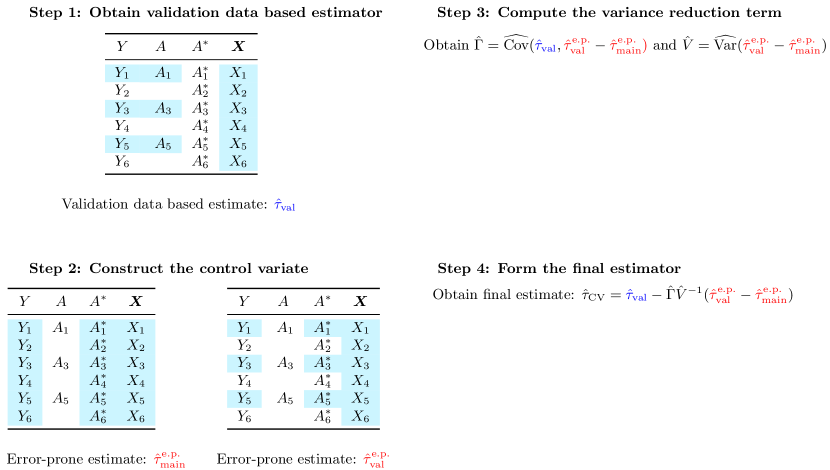
Figure 2: Illustration of the control variates method.

3.2 Obtaining the Components of the Control Variates Estimator

To consistently estimate $\tau_{\text{TATE}}$ in this setting, we propose the use of doubly-robust estimators developed in the generalizability and transportability literature that leverage semiparametric efficiency theory. Specifically, we explore the efficient generalization estimators initially proposed by Dahabreh et al. (2019). These estimators leverage the observation that under Assumptions 1-3 and Assumptions 5.a-5.b, $\tau_{\text{TATE}}$ can be identified by the G-computation functional outlined in Equation (2). The aforementioned references have demonstrated the application of the efficient influence function derived from the functional displayed in Equation (2), implying the doubly-robust estimator

$${\hat{\tau}_{\text{val}}=\frac{1}{n}\sum_{i=1}^{n}\left[\frac{I(A_{i}=1,S_{i}=1)(Y_{i}-\hat{\mu}_{1}(\bm{X}_{i}))}{\hat{\kappa}(\bm{X}_{i})\hat{\pi}(\bm{X}_{i})}-\frac{I(A_{i}=0,S_{i}=1)(Y_{i}-\hat{\mu}_{0}(\bm{X}_{i}))}{\hat{\kappa}(\bm{X}_{i})(1-\hat{\pi}(\bm{X}_{i}))}+\hat{\mu}_{1}(\bm{X}_{i})-\hat{\mu}_{0}(\bm{X}_{i})\right]},$$ (6)

where $\mu_{a}(x)\overset{\text{def}}{=}\mathbb{E}(Y|\bm{X}=x,A=a,S=1)$ and $\pi(x)\overset{\text{def}}{=}\mathbb{P}(A=1|\bm{X}=\bm{x},S=1)$ are estimated with the validation data, and $\kappa(x)\overset{\text{def}}{=}\mathbb{P}(S=1|\bm{X}=\bm{x})$ is estimated over the full sample. When the two-phase sampling probabilities $\kappa(\bm{X})$ are controlled by the researcher, one can either substitute in its true values or estimate it for further efficiency gains. Notably, this approach does not require knowledge of the underlying measurement error model, and accommodates both Assumption 4 and 5.a.

Similar to the construction of $\hat{\tau}_{\text{val}}$, one can make an analogous adjustment to $\hat{\tau}_{\text{val}}^{\text{e.p.}}$ to ensure the control variate is consistent for 0, by recalling equality of the two functionals displayed in Equation (3). Recall that the key requirement for the control variate is not that this functional represents a causal effect, but rather that we can construct estimators in both the main and validation data that are both consistent for the same fixed quantity. Notice that the left-hand side of Equation (3) can be consistently estimated using the same efficient generalization strategy described above with

$${\hat{\tau}_{\text{val}}^{\text{e.p.}}=\frac{1}{n}\sum_{i=1}^{n}\left[\frac{I(A_{i}^{*}=1,S_{i}=1)(Y_{i}-\hat{\mu}^{\text{e.p.}}_{1}(\bm{X}_{i}))}{\hat{\kappa}(\bm{X}_{i})\hat{\pi}^{\text{e.p.}}(\bm{X}_{i})}-\frac{I(A_{i}^{*}=0,S_{i}=1)(Y_{i}-\hat{\mu}^{\text{e.p.}}_{0}(\bm{X}_{i}))}{\hat{\kappa}(\bm{X}_{i})(1-\hat{\pi}^{\text{e.p.}}(\bm{X}_{i}))}+\hat{\mu}^{\text{e.p.}}_{1}(\bm{X}_{i})-\hat{\mu}^{\text{e.p.}}_{0}(\bm{X}_{i})\right]},$$ (7)

where $\mu^{\text{e.p.}}_{a}(x)\overset{\text{def}}{=}\hat{\mathbb{E}}(Y|\bm{X}=x,A^{*}=a,S=1)$ and $\pi^{\text{e.p.}}(\bm{x})\overset{\text{def}}{=}\hat{\mathbb{P}}(A^{*}=1|\bm{X}=\bm{x},S=1)$ are the error-prone CATE and propensity score models. The right-hand side of (3) can be consistently estimated using the main data with the standard AIPW estimator

$${\hat{\tau}_{\text{main}}^{\text{e.p.}}=\frac{1}{n}\sum_{i=1}^{n}\left[\frac{I(A_{i}^{*}=1)(Y_{i}-\hat{m}^{\text{e.p.}}_{1}(\bm{X}_{i}))}{\hat{g}^{\text{e.p.}}(\bm{X}_{i})}-\frac{I(A_{i}=0)(Y_{i}-\hat{m}^{\text{e.p.}}_{0}(\bm{X}_{i}))}{1-\hat{g}^{\text{e.p.}}(\bm{X}_{i})}+\hat{m}^{\text{e.p.}}_{1}(\bm{X}_{i})-\hat{m}^{\text{e.p.}}_{0}(\bm{X}_{i})\right]},$$ (8)

where $m^{\text{e.p.}}_{a}(\bm{X})\overset{\text{def}}{=}\mathbb{E}[Y|A^{*}=a,\bm{X}]$ and $g^{\text{e.p.}}(\bm{X})\overset{\text{def}}{=}\mathbb{P}(A^{*}=1|\bm{X})$ are error-prone analogues of the full-data CATE and propensity score functions $m_{a}(\bm{X})$ and $g(\bm{X})$ that do not condition on $S=1$. Importantly, we have not made any functional assumptions about the measurement error process.

3.3 Theoretical Results

Given a means for constructing each component of $\hat{\tau}_{\text{CV}}$, we can turn our attention to inference. The following Theorem, whose proof is provided in the Supplementary Materials, characterizes the asymptotic distribution of the control variates estimator (restricting consideration to RAL estimators) under Assumptions 1-3 and 5.a-5.b:

Theorem 1

Let $\hat{\tau}_{\text{val}}$, $\hat{\tau}_{\text{val}}^{\text{e.p.}}$ and $\hat{\tau}_{\text{main}}^{\text{e.p.}}$ be RAL estimators satisfying (4) with corresponding influence functions $\varphi^{*}(A,\bm{X},Y),\phi^{*}(A^{*},\bm{X},Y)$ and $\phi(A^{*},\bm{X},Y)$, respectively. For suitable estimators, under Assumptions 1-3 and Assumptions 5.a-5.b we have that $\sqrt{n}(\hat{\tau}_{\text{CV}}-\tau_{\text{TATE}})\overset{D}{\rightarrow}N(0,v-\Gamma^{2}/V)$ where

$$(1)\ v=\text{Var}(\varphi^{*}(A,\bm{X},Y)),$$

$$(2)\ V=\text{Var}(\phi^{*}(A^{*},\bm{X},Y)-\phi(A^{*},\bm{X},Y)),\text{ and }$$

$$(3)\ \Gamma=\text{Cov}(\varphi^{*}(A,\bm{X},Y),\phi^{*}(A^{*},\bm{X},Y)-\phi(A^{*},\bm{X},Y)).$$

There are multiple immediate consequences resulting from Theorem 1. First, notice that for a given set of RAL estimators used to construct $\hat{\tau}_{\text{CV}}$, $v,\Gamma$ and $V$ can be consistently estimated by their sample analogues, substituting in estimated values for the influence functions $\varphi^{*}(A,\bm{X},Y),\phi^{*}(A^{*},\bm{X},Y)$ and $\phi(A^{*},\bm{X},Y)$. We additionally provide a bootstrap procedure, similar to the one developed by Guo et al. (2021), in the Supplementary Materials. Second, the asymptotic normality of $\hat{\tau}_{\text{CV}}$ enables straightforward inference and means for constructing confidence intervals, while also analytically quantifying the efficiency gain enjoyed from implementing the control variates method.

A more subtle property of our proposed procedure is that when $\hat{\tau}_{\text{val}},\hat{\tau}_{\text{val}}^{\text{e.p.}}$ and $\hat{\tau}_{\text{main}}^{\text{e.p.}}$ are all obtained through doubly-robust estimators, such as the ones outlined in Section 3.2, then $\hat{\tau}_{\text{CV}}$ will inherit the double robustness properties of its component estimators. Specifically, $\hat{\tau}_{\text{CV}}$ will enjoy the consistency and, in our view more crucially, rate robustness conditions of its underlying components. This implies that if one wishes to make minimal assumptions about the underlying data-generating model and estimate all nuisance functions with flexible data-adaptive methods that themselves have slower rates of convergence, then the resulting control variates estimator can still achieve parametric $\sqrt{n}$ rates of convergence. We provide additional information on the precise robustness conditions of $\hat{\tau}_{\text{CV}}$ in the Supplementary Materials.

3.4 Complex Validation Data Sampling Schemes

When researchers have control over which subjects to sample into the validation data, one may choose to adopt complex sampling rules that depend not only on the baseline covariates, but also the error-prone exposures $A^{*}$ and the observed outcomes $Y$. Biased sampling schemes have a long history in two-phase sampling designs (Breslow and Chatterjee 1999; Neyman 1938), and can allow for efficiency gains by over-sampling observations that contribute higher degrees of information about the target estimand, particularly in scenarios where the exposure or outcome of interest is rare. Figure 3 displays a causal diagram consistent with such a biased sampling scheme.

Figure 3: Selection into the validation data is random conditional on all initially observed data.

For study designs where the researcher has control over the sampling mechanism into the validation data, the control variates method can be extended to accommodate biased sampling schemes. Specifically, suppose selection into the validation data is determined according to a known sampling function $\kappa(\bm{X},A^{*},Y)\overset{\text{def}}{=}\mathbb{P}(S=1|\bm{X},A^{*},Y)$, and Assumptions 1-3 hold. Notably, this sampling strategy implies $A\perp\!\!\!\perp S|\bm{X},A^{*},Y$. To construct $\hat{\tau}_{\text{val}}$ and $\hat{\tau}_{\text{val}}^{\text{e.p.}}$, we propose the use of estimators based on weighted uncentered influence functions developed in the two-phase sampling literature (Rose and van der Laan 2011)

$$\hat{\varphi}^{\text{IPSW}}(\bm{Z},A,S) =\frac{S}{\kappa(\bm{Z})}\left\{\hat{m}_{1}(\bm{X})-\hat{m}_{0}(\bm{X})+\left(\frac{A}{\hat{g}(\bm{X})}-\frac{1-A}{1-\hat{g}(\bm{X})}\right)\hat{m}_{A}(\bm{X})\right\}$$

$$\hat{\phi}^{\text{IPSW,e.p.}}(\bm{Z},S) =\frac{S}{\kappa(\bm{Z})}\left\{\hat{m}^{\text{e.p.}}_{1}(\bm{X})-\hat{m}^{\text{e.p.}}_{0}(\bm{X})+\left(\frac{A^{*}}{\hat{g}^{\text{e.p.}}(\bm{X})}-\frac{1-A^{*}}{1-\hat{g}^{\text{e.p.}}(\bm{X})}\right)\hat{m}^{\text{e.p.}}_{A^{*}}(\bm{X})\right\},$$

where $\bm{Z}=(\bm{X},A^{*},Y)$. The above full-data nuisance functions $m_{a},m_{a}^{\text{e.p.}},g$ and $g^{\text{e.p.}}$, defined in Section 3.2, can be estimated through regression methods by adding weights $S/\kappa(\bm{Z})$ to the underlying loss function (Rose and van der Laan 2011). Let $\hat{\tau}_{\text{val}}^{\text{IPSW}}=\frac{1}{n}\sum_{i=1}^{n}\hat{\varphi}^{\text{IPSW}}(\bm{Z}_{i},A_{i},S_{i})$ and $\hat{\tau}_{\text{val}}^{\text{IPSW,e.p.}}=\frac{1}{n}\sum_{i=1}^{n}\hat{\phi}^{\text{IPSW,e.p.}}(\bm{Z}_{i},S_{i})$, and let $\phi^{\text{e.p.}}(\bm{Z})$ denote the un-weighted analogue of $\phi^{\text{IPSW,e.p.}}(\bm{Z}_{i},S_{i})$. The following Theorem summarizes how these two estimators can be used to construct a control variates estimator in this setting.

Theorem 2

Suppose the sampling probabilities $\kappa(\bm{Z})$ are known and Assumptions 1-3 hold. Then, under regularity conditions outlined in the Supplementary Materials, we have that

1. $\hat{\tau}_{\text{val}}^{\text{IPSW}}$ is asymptotically linear for $\tau_{\text{TATE}}$, with influence function $\varphi^{\text{IPSW}}(\bm{Z},A,S)-\tau_{\text{TATE}}$, and

2. $\hat{\tau}_{\text{val}}^{\text{IPSW,e.p.}}$ is asymptotically linear for $\tau^{\text{e.p.}}$, with influence function $\phi^{\text{IPSW}}(\bm{Z},S)-\tau^{\text{e.p.}}$.

3. When $\hat{\tau}_{\text{main}}^{\text{e.p.}}$ is obtained as in (8), we have that

   $$\sqrt{n}\begin{pmatrix}\hat{\tau}_{\text{val}}^{\text{IPSW}}-\tau_{\text{TATE}}\\ \hat{\tau}^{\text{IPSW,e.p.}}_{\text{val}}-\hat{\tau}^{\text{e.p.}}_{\text{main}}\end{pmatrix}\overset{D}{\rightarrow}N\left(\bm{0},\bm{\Sigma}\right),\ \ \ \bm{\Sigma}=\begin{pmatrix}v^{\text{IPSW}}&\Gamma^{\text{IPSW}}\\ \Gamma^{\text{IPSW}}&V^{\text{IPSW}}\end{pmatrix},$$ (9)

$$\Gamma^{\text{IPSW}} =\text{Cov}\left([S/\kappa(\bm{Z})-1]\phi^{\text{e.p.}}(\bm{Z},S),\varphi^{\text{IPSW}}(\bm{Z},A,S)\right);$$

$$V^{\text{IPSW}} =\text{Var}\left([S/\kappa(\bm{Z})-1]\phi^{\text{e.p.}}(\bm{Z},S)\right).$$

The proof of Theorem 2 is provided in the Supplementary Materials. Our result extends findings in Yang and Ding (2019) by relaxing the requirement that the true CATE and propensity score functions lay in parametric modeling classes. An immediate corollary of Theorem 2 is that control variates estimators of the form $\hat{\tau}_{\text{CV}}=\hat{\tau}_{\text{val}}^{\text{IPSW}}-\hat{\Gamma}^{\text{IPSW}}/\hat{V}^{\text{IPSW}}(\hat{\tau}_{\text{val}}^{\text{IPSW,e.p.}}-\hat{\tau}_{\text{main}}^{\text{e.p.}}),$ where $\hat{\tau}_{\text{main}}^{\text{e.p.}}$ is obtained as in (8), will be consistent for $\tau_{\text{TATE}}$. Further, the asymptotic linearity of all three component estimators implies one can estimate $\Gamma^{\text{IPSW}}$ and $V^{\text{IPSW}}$ through the influence functions of each estimator.

4 Simulation Study

4.1 Setting

To investigate the performance of the control variates method in finite-sample settings, we conducted an extensive simulation exercise. We implemented the control variates method with the doubly-robust component estimators for $\hat{\tau}_{\text{val}},\hat{\tau}_{\text{val}}^{\text{e.p.}}$ and $\hat{\tau}_{\text{main}}^{\text{e.p.}}$ outlined in Section 3.2. We compared the control variates estimator to an oracle (best case) AIPW estimator where one has access to the true $A$ for every observation, a naïve AIPW estimator that ignores measurement error and uses $A^{*}$ in place of $A$, the generalization estimator outlined in (6), a validation data only AIPW estimator and multiple imputation for measurement error (denoted MIME), the current standard approach taken for addressing measurement error with validation data (Webb-Vargas et al. 2017; Josey et al. 2023). We emphasize that the generalization estimator (6) $\hat{\tau}_{\text{val}}$ is the initial consistent estimator used in forming the control variates estimator, whose variance is reduced by the inclusion of the control variate term. For each estimator, we estimated all underlying nuisance models with a Super Learner (Van der Laan et al. 2007). Full details are provided in the Supplementary Materials.

We consider two general scenarios: 1) the validation samples are selected completely at random, and 2) the validation samples are selected conditionally as a function, which we treat as unknown, of the measured covariates $\bm{X}$. Within each scenario, we examined how the competing estimators perform under varying levels of measurement error severity and by altering the relative sizes of the validation data, $\rho\overset{\text{def}}{=}\mathbb{P}(S=1)$. We generated $5{,}000$ datasets of $n=5{,}000$ observations through the following process:

$$\bm{X}_{i} \sim N(\bm{1},\bm{\Sigma}_{\bm{X}}) (\text{Covariates});$$

$$A_{i}|\bm{X}_{i} \sim\text{Bernoulli}(\pi(\bm{X}_{i})),\enskip\pi(\bm{X}_{i})=\text{expit}(\alpha_{0}+\bm{X}_{i}^{\top}\bm{\alpha}) (\text{Exposure});$$

$$A_{i}^{*}|A_{i} \sim\text{Bernoulli}(p_{i}),\ p_{i}=A_{i}\delta+(1-A_{i})\zeta (\text{Measurement});$$

$$S_{i}|\bm{X}_{i} \sim\text{Bernoulli}(\kappa(\bm{X}_{i})),\enskip\kappa(\bm{X}_{i})=\frac{\rho\cdot\text{expit}(\eta_{0}+\bm{X}_{i}^{\top}\bm{\eta})}{\frac{1}{n}\sum_{k=1}^{n}\text{expit}(\eta_{0}+\bm{X}_{k}^{\top}\bm{\eta})} (\text{Val. data selection});$$

$$Y_{i}|A_{i},\bm{X}_{i} \sim N(\mu(\bm{X}_{i}),\varepsilon),\enskip\mu(\bm{X}_{i})=\beta_{0}+\tau A_{i}+\bm{X}_{i}^{\top}\bm{\beta}+A_{i}\bm{X}_{i}^{\top}\bm{\gamma} (\text{Outcome}).$$

We performed multiple imputation using the mice package in R (Van Buuren and Groothuis-Oudshoorn 2011), generating $10$ imputed datasets through predictive mean matching (Little 1988) and implementing Rubin’s combining rules to obtain our final treatment effect and variance estimates. Predictive mean matching is the default imputation model option in mice, and has been demonstrated to flexibly account for complex missing data patterns (Kleinke 2017). We implement the control variates method with the controlVariatesME R package, which we developed to facilitate use of our proposed methods. In implementing the control variates method, we use the asymptotic expressions from Theorem 1 to estimate $\Gamma$ and $V$. Full details on the simulation design and replication code are included in the Supplementary Material.

4.2 Results

Figures 4 and 5 display results from the simulation in settings where the validation data is obtained completely at random and conditionally at random given $\bm{X}$, respectively. We report the percent bias, 95% confidence interval coverage rate, and root mean square error (RMSE) of each estimator under both sampling scenarios, against varying sensitivity levels $\delta$—a measure of measurement error severity —and relative sizes of the validation data.

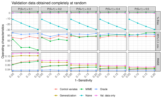
Figure 4: Percent bias, 95% CI coverage and RMSE of each method by sensitivity, relative size of validation data to main data. Validation data is obtained completely at random. RMSE is only displayed for estimators that are not severely biased, to avoid distorting the scale. Simulation results are averaged over $5000$ iterations, fixing $n_{\text{main}}=5000$.

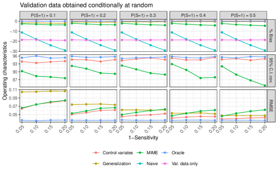
Figure 5: Percent bias, 95% CI coverage and RMSE of each method by sensitivity and relative size of validation data to main data. Validation data is obtained conditionally on $\bm{X}$, inducing covariate shift between the main and validation data. RMSE is only displayed for estimators that are not severely biased, to avoid distorting the scale. Simulation results are averaged over $5000$ iterations, fixing $n_{\text{main}}=5000$.

Beginning with Figure 4, there are three key takeaways. First, we see that in all settings, the naïve estimator is considerably biased, highlighting the general need to account for exposure measurement error. Second, we see that multiple imputation and the control variates method both offer substantial RMSE reduction relative to the validation data only estimator across increasingly severe measurement error, regardless of the validation data size, but particularly as smaller portions of the main sample are included in the validation sample. Finally, due to a minor mis-specification in the predictive mean matching imputation model, multiple imputation is slightly biased, leading to undercoverage of the nominal 95% confidence level.
In Figure 5, where the validation data is obtained at random but inclusion occurs conditionally on the covariates, there are again three key takeaways. First, naïvely using a validation data only estimator, which ignores covariate shift between the main and validation data, leads to substantial bias. Second, multiple imputation exhibits minor degrees of bias that hampers its coverage rates. Intuitively, the introduction of covariate shift further complicates the underlying true—but unknown—imputation model, with the resulting misspecification of a predictive mean matching approach propagating into the final estimate. Finally, we see that the control variates estimator is again unbiased but in this scenario it outperforms MIME in terms of RMSE due to the misspecification bias of the latter estimator under this validation sampling scenario.

5 Extension: Surrogate Outcome Measurements

So far, we have restricted our focus to applications involving an error-prone exposure. The control variates approach can also be used to accommodate measurement error in the outcome of interest. More generally, the control variates method can be adapted for scenarios where there are multiple surrogate outcomes available for the entire dataset, with the true outcome of interest only being available for a subset of observations. Surrogate outcome problems commonly arise in scenarios where the primary outcome of interest is expensive to measure and hence available for only a subset of all subjects, while inexpensive proxies are available for all subjects. Surrogate outcome problems have been extensively studied in causal inference applications (see, e.g. Kallus and Mao 2020 and Athey et al. 2016).

For simplicity, we consider the scenario where data are collected from a single source from which there are $K$ surrogate outcomes available for the entire dataset, with the true outcome only available for a subset of the data that is selected completely at random and the true exposure measurements available for every observation. Adapting the procedure to simultaneously accommodate exposure measurement error is a straightforward extension of the earlier methods. Let $Z_{1},\dots,Z_{K}$ denote the $K$ surrogate outcomes, and let the ATE of the exposure on the $k$-th surrogate outcome be defined as $\psi_{k}\overset{\text{def}}{=}\mathbb{E}(Z_{k}(1)-Z_{k}(0))$ recalling that interest lies in the ATE of the exposure $A$ on the outcome of interest $Y$, $\tau_{\text{TATE}}\overset{\text{def}}{=}\mathbb{E}(Y(1)-Y(0))$. As noted in Kallus and Mao (2020), outcome measurement error can be viewed as a special case of the surrogate outcome problem, where $K=1$ and $Z_{1}$ denotes error-prone measurements of the true outcome of interest $Y$.

As there are $K$ surrogates, one can construct a $K$-dimensional control variate, where each component of the control variate can be constructed as follows: 1) Using only the subset of data with primary outcome measurements, obtain an estimate of $\tau_{\text{TATE}}$, denoted $\hat{\tau}$, 2) With the entire sample, obtain an estimate of $\tau_{k}$, denoted $\hat{\tau}_{k,\text{main}}$, and 3) Form the $k$-th control variate by taking the difference $\hat{\tau}_{k,\text{main}}-\hat{\tau}_{k\text{val}}$. The resulting control variates estimator has the asymptotic distribution

$$\sqrt{n}\begin{pmatrix}\hat{\tau}_{\text{val}}-\tau_{\text{TATE}}\\ \hat{\tau}_{1,\text{val}}-\hat{\tau}_{1,\text{main}}\\ \vdots\\ \hat{\tau}_{K,\text{val}}-\hat{\tau}_{K,\text{main}}\end{pmatrix}\overset{D}{\rightarrow}N\left(\bm{0},\bm{\Sigma}\right),\ \ \ \bm{\Sigma}=\begin{pmatrix}v&\Gamma^{\top}\\ \Gamma&V\end{pmatrix},$$

and the final estimator of $\tau_{\text{TATE}}$ takes the form

$$\hat{\tau}_{\text{CV}}\overset{\text{def}}{=}\hat{\tau}_{\text{val}}-\hat{\Gamma}^{\top}\hat{V}^{-1}[\hat{\tau}_{1,\text{val}}-\hat{\tau}_{1,\text{main}},\ \dots\ ,\hat{\tau}_{K,\text{val}}-\hat{\tau}_{K,\text{main}}].$$

The availability of multiple surrogate outcomes allows for additional opportunities to reduce the variance of the validation data estimator.

6 Data Example

We applied the control variates method to electronic health record (EHR) data from the Vanderbilt Comprehensive Care Clinic (VCCC), an outpatient facility serving people living with HIV. The VCCC data has been featured in several works focusing on measurement error-correction methods, including Oh et al. (2021); Giganti et al. (2020) and Amorim et al. (2021). Data were collected on numerous baseline characteristics at each patient’s initial visit, as well as clinical data at all follow-up visits. Continuous characteristics, denoted $\bm{C}_{i}$, included age at first visit, while discrete characteristics $\bm{X}_{i}$ included risk factors such as injection drug use, and demographic characteristics including sex, race and ethnicity. See Web Appendix Table 2 for additional information on all relevant variables.

The VCCC validated error-prone records for all 4,217 patients, resulting in an initial unvalidated dataset and a corresponding fully-validated dataset while revealing considerable error in numerous EHR-derived variables. Among the severely error-prone variables was the occurrence of an AIDS-defining event (ADE) prior to first visit, an indicator of severely delayed initiation of treatment. Access to the complete set of both validated and error-prone ADE measurements provides an ideal scenario for examining the real-world performance of the control variates method relative to naïve and validation-data only estimators.

To evaluate the control variates method, we emulate a scenario in which a researcher seeks to estimate the average causal effect of having suffered an ADE at baseline ($A$), which possesses initial error-prone measurements $A^{*}$, on the 5-year post-baseline risk of death ($Y$) among patients with no history of antiretroviral therapy (ART) use prior to initiating care with the VCCC. Using the validated ART data to exclude patients who initiated ART prior to enrollment at the VCCC—a common exclusion criterion in HIV studies—1,907 patients remained. The misclassification rate of ADE among these 1,907 patients was 0.096, where much of this misclassification was due to false positives. Notably, the error-prone ADE indicator exhibited a false positive rate of 0.420, with a more modest false negative rate of 0.031. Given that pre-baseline ADEs were relatively infrequent in the validated data, with a prevalence of 0.123, this suggests that naïvely using the error-prone ADE indicators can result in substantial bias.

With access to validated ADE indicators for every patient, we can examine the performance of the control variates estimator under different relative sizes of the validation data by artificially ignoring varying proportions of validation data, pretending we do not have access to the remaining validated ADE indicators. To do this, we considered the same set of relative sizes as in the simulation exercise. At each validation size, we created 1,000 hypothetical internal validation datasets via simple random sampling without replacement from the original, full validation dataset. To ensure we know the true underlying causal parameter, we simulated a synthetic 5-year survival outcome by (1) fitting a logistic regression model

$$\mathbb{E}[Y_{i}|A_{i},\bm{X}_{i},\bm{C}_{i}]=\text{expit}(\alpha A_{i}+A_{i}\bm{X}_{i}^{\top}\bm{\gamma}+\bm{C}_{i}^{\top}\bm{\beta})$$ (10)

using the validated ADE measurements and (2) at each simulation iteration, used the fitted model (10) to a generate a new realization of the synthetic outcome so that each of the 1,000 simulated internal validation datasets has an accompanying synthetic survival outcome. We implemented the control variates method using each of the hypothetical validation datasets, with $\hat{\tau}_{\text{val}}$, $\hat{\tau}_{\text{val}}^{\text{e.p.}}$ and $\hat{\tau}_{\text{main}}^{\text{e.p.}}$ estimated via the methods outlined in Section 3.1. We compare the control variates estimator to the generalization estimator $\hat{\tau}_{\text{val}}$, as well as the same naïve and oracle AIPW estimators outlined in Section 4. All nuisance models were estimated with a Super Learner that adjusts for the baseline factors $\bm{X}_{i}$ and $\bm{C}_{i}$. See the Supplementary Materials for further details on our implementation and Super Learner libraries.

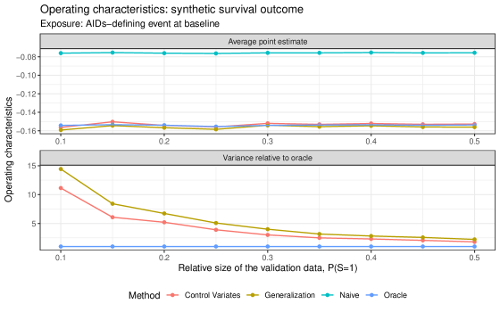
Figure 6: Results from the VCCC data application.

The results of our analysis are displayed in Figure 6. We present the average point estimate of each method and their relative efficiency compared to the oracle estimator at each value of $\rho$ considered. Similar to the findings from the simulation study, we see that ignoring measurement error generates substantial bias—on the order of 50% in this example—while the generalization and control variates estimators are unbiased by design. We also observe that the control variates estimator provides considerable variance reduction relative to the validation data based estimator, improving the efficiency of the validation data based estimator by roughly 20% across all validation sizes considered. This reduction in variance is notable since exposure measurement validation will tend to be costly in practice. Our results suggests that by applying our proposed methods, one can attain efficiency levels that would otherwise require additional expensive data validation.

7 Discussion

Research at the intersection of measurement error and causal inference is a relatively new endeavour. Nevertheless, there is a growing need for flexible, modern methods for the estimation of causal effects that can accommodate various study designs while addressing measurement error. In this paper, we make contributions to this area of research by introducing the control variates estimator as a means for addressing exposure measurement error, under two-phase sampling data collection processes. Theory and our simulation studies show that relative to multiple imputation, our proposed method is more robust to model misspecification, as multiple imputation requires consistent estimation of the exposure imputation model while the control variates method does not require one to specify an imputation model. We also demonstrate the flexibility of our proposed approach, showing its ability to address related problems including multiple surrogate outcomes, and complex validation data sampling schemes. Using recent developments from the generalizability and transportability literature, we extended earlier work by Yang and Ding (2019), deriving the asymptotic distribution of a generic control variates estimator that makes use of efficient generalization and transportation estimation procedures. Theory, our simulation study and data application all demonstrate that the control variates method can substantially reduce the number of validation samples required to achieve a desired level of efficiency.

There are many avenues for future study mentioned intermittently throughout this article. While the simulation study provides preliminary insights into the performance of the control variates estimator relative to common approaches to measurement error correction, it would be valuable to consider more complicated data-generating processes and, in particular, a more exhaustive set of measurement error mechanisms. Further, while the focus of this paper is on measurement error in the exposure of interest, the control variates method naturally extends to scenarios where there is measurement error in the outcome, or scenarios where the outcome is partially missing with full information on surrogate outcomes. Considerations of this extension, while highlighted briefly in Section 5, and comparison with methods like multiple imputation and the method described in Kallus and Mao (2020), would be valuable for scientists trying to discern the best method for their analytical challenges.

Acknowledgements

This work was funded by the National Institute of Health (NIH) grants T32AI007358, K01ES032458, R37AI131771 and P30AI110527.

Supplementary Material for “Flexible and Efficient Estimation of Causal Effects with Error-Prone Exposures: A Control Variates Approach for Measurement Error”
by K. Barnatchez, R. Nethery, B. Shepherd, G. Parmigiani, and K. Josey

Web Appendix A: Proofs

Proof of Theorem 1

Since $\hat{\tau}_{\text{val}},\hat{\tau}_{\text{val}}^{\text{e.p.}}$ and $\hat{\tau}_{\text{main}}^{\text{e.p.}}$ are all RAL, we have

$$\sqrt{n}(\hat{\tau}_{\text{val}}-\tau_{\text{TATE}}) =\frac{1}{\sqrt{n}}\sum_{i=1}^{n}\varphi^{*}(A_{i},\bm{X}_{i},Y_{i},S_{i})+o_{\mathbb{P}}(1);$$

$$\sqrt{n}(\hat{\tau}^{\text{e.p.}}_{\text{main}}-\tau_{\text{e.p.}}) =\frac{1}{\sqrt{n}}\sum_{i=1}^{n}\phi(A_{i}^{*},\bm{X}_{i},Y_{i})+o_{\mathbb{P}}(1);$$

$$\sqrt{n}(\hat{\tau}^{\text{e.p.}}_{\text{val}}-\tau_{\text{e.p.}}) =\frac{1}{\sqrt{n}}\sum_{i=1}^{n}\phi^{*}(A_{i}^{*},\bm{X}_{i},Y_{i},S_{i})+o_{\mathbb{P}}(1).$$

This implies

$$\sqrt{n}(\hat{\tau}^{\text{e.p.}}_{\text{val}}-\hat{\tau}^{\text{e.p.}}_{\text{main}}) =\frac{1}{\sqrt{n}}\sum_{i=1}^{n}\left[\phi^{*}(A_{i}^{*},\bm{X}_{i},Y_{i})-\phi(A_{i}^{*},\bm{X}_{i},Y_{i})\right].$$

Since all observations are i.i.d. we have that

$$\text{Var}\left(\frac{1}{\sqrt{n}}\sum_{i=1}^{n}\phi^{*}(A_{i}^{*},\bm{X}_{i},Y_{i})\right) =\text{Var}(\phi^{*}(A^{*},\bm{X},Y))=v,\text{ and}$$

$$\text{Var}\left(\frac{1}{\sqrt{n}}\sum_{i=1}^{n}\left[\phi^{*}(A_{i}^{*},\bm{X}_{i},Y_{i})-\phi(A_{i}^{*},\bm{X}_{i},Y_{i})\right]\right) =\text{Var}(\phi^{*}(A^{*},\bm{X},Y)-\phi(A^{*},\bm{X},Y))=V,$$

Through similar reasoning,

$$\text{Cov}\left(\sqrt{n}(\hat{\tau}_{\text{val}}-\tau_{\text{TATE}}),\sqrt{n}(\hat{\tau}_{\text{val}}^{\text{e.p.}}-\hat{\tau}^{\text{e.p.}}_{\text{main}})\right) =\text{Cov}(\varphi^{*}(A_{i},\bm{X}_{i},Y_{i},S_{i}),\phi^{*}(A^{*},\bm{X},Y)-\phi(A^{*},\bm{X},Y))$$

$$=\Gamma$$

Let $\Gamma$ and $v$ be estimated by their sample analogues. Recalling $\hat{\tau}_{\text{CV}}=\hat{\tau}_{\text{val}}-\hat{\Gamma}/\hat{V}(\hat{\tau}_{\text{val}}^{\text{e.p.}}-\hat{\tau}_{\text{main}}^{\text{e.p.}})$, and that all 3 component estimators are RAL, asymptotic normality directly follows by Slutsky’s Theorem. To establish the asymptotic variance of $\hat{\tau}_{\text{CV}}$, notice that asymptotically

$$\text{Var}(\hat{\tau}_{\text{CV}}) =\text{Var}(\hat{\tau}_{\text{val}})+(\Gamma/V)^{2}\text{Var}(\hat{\tau}_{\text{val}}^{\text{e.p.}}-\hat{\tau}_{\text{main}}^{\text{e.p.}})-2\Gamma/V\text{Cov}(\hat{\tau}_{\text{val}},(\hat{\tau}_{\text{val}}^{\text{e.p.}}-\hat{\tau}_{\text{main}}^{\text{e.p.}}))$$

$$=\text{Var}(\hat{\tau}_{\text{val}})+\frac{1}{n}\Gamma^{2}/V-\frac{1}{n}2\Gamma^{2}/V$$

$$=\frac{1}{n}\left(v-\Gamma^{2}/V\right).$$

Proof of Theorem 2

Asymptotic Linearity of $\hat{\tau}_{\text{val}}^{\text{IPSW}}$ and $\hat{\tau}_{\text{val}}^{\text{IPSW,e.p.}}$

Without loss of generality, we will focus our attention on $\hat{\tau}_{\text{val}}$. Analogous reasoning will establish all results for $\hat{\tau}_{\text{val}}^{\text{e.p.}}$. First, suppose the following regularity conditions hold:

1. $||\hat{m}_{a}-m_{a}||=o_{\mathbb{P}}(n^{-1/4})$

2. $||\hat{g}-g||=o_{\mathbb{P}}(n^{-1/4})$

3. $||\hat{m}_{a}^{\text{e.p.}}-m_{a}^{\text{e.p.}}||=o_{\mathbb{P}}(n^{-1/4})$

4. $||\hat{g}^{\text{e.p.}}-g^{\text{e.p.}}||=o_{\mathbb{P}}(n^{-1/4})$

To satisfy empirical process conditions we additionally assume that all nuisance models are fit in a separate held-out sample (Kennedy 2020). One can implement cross-fitting methods (Zivich and Breskin 2021) to recover full efficiency of the resulting estimators.

We aim to show that $\hat{\tau}_{\text{val}}^{\text{IPSW}}$ is asymptotically linear for $\tau_{\text{TATE}}$. Recall that

$$\hat{\varphi}^{\text{IPSW}}(Y,A,\bm{X},S)=\frac{S}{\kappa(\bm{X},A,Y,S)}\left\{\hat{m}_{1}(\bm{X})-\hat{m}_{0}(\bm{X})+\left(\frac{A}{\hat{g}(\bm{X})}-\frac{1-A}{1-\hat{g}(\bm{X})}\right)\hat{m}_{A}(\bm{X})\right\}.$$

Let

$$\hat{\phi}(Y,A,\bm{X},S)=\hat{m}_{1}(\bm{X})-\hat{m}_{0}(\bm{X})+\left(\frac{A}{\hat{g}(\bm{X})}-\frac{1-A}{1-\hat{g}(\bm{X})}\right)\hat{m}_{A}(\bm{X}),$$

denote the uncentered efficient influence curve of the ATE functional $\psi=\mathbb{E}[\mathbb{E}(Y|A=1,\bm{X})-\mathbb{E}(Y|A=0,\bm{X})]$ under the full data structure. Then, the efficient influence curve under the observed data structure, denoted $\chi(\bm{O})$, can be written as a function of the underlying full-data influence function (Rose and van der Laan 2011; Levis et al. 2022):

$$\chi(\bm{O}) =\frac{S}{\kappa(\bm{X},A^{*},Y)}\phi(Y,A,\bm{X},S)-\left(\frac{S}{\kappa(\bm{X},A^{*},Y)}-1\right)\mathbb{E}[\phi(Y,A,\bm{X},S)|\bm{X},A^{*},Y]-\psi$$

$$=\varphi^{\text{IPSW}}(Y,A,A^{*},\bm{X},S)-\left(\frac{S}{\kappa(\bm{X},A^{*},Y)}-1\right)\mathbb{E}[\phi(Y,A,\bm{X},S)|\bm{X},A^{*},Y]-\psi.$$

Consider the estimator

$$\hat{\psi}=\frac{1}{n}\sum_{i=1}^{n}\left(\hat{\varphi}^{\text{IPSW}}(Y_{i},A_{i},A_{i}^{*},\bm{X}_{i},S_{i})-\left(\frac{S_{i}}{\kappa(\bm{X}_{i},A_{i}^{*},Y_{i})}-1\right)\hat{\mathbb{E}}[\phi(Y_{i},A_{i},\bm{X}_{i},S_{i})|\bm{X}_{i},A_{i}^{*},Y_{i}]\right),$$

and further define

$$\Phi(\bm{X},A^{*},Y)=\mathbb{E}[\phi(Y,A,\bm{X},S)|\bm{X},A^{*},Y].$$ (A1)

Through Proposition 5 of Levis et al. (2022), it has been shown that two-stage sampling estimators of this form have the following bias structure:

$$\mathbb{E}[\hat{\psi}-\tau_{\text{TATE}}]=O_{\mathbb{P}}\left(\frac{1}{\sqrt{n}}+||\hat{m}-m||\cdot||\hat{g}-g||+||\hat{\kappa}-\kappa||\cdot||\hat{\Phi}-\Phi||\right).$$ (A2)

Crucially, (A2) implies that under the earlier regularity conditions 1 and 2, $\hat{\psi}$ is asymptotically linear with influence function $\chi(\bm{O})$, since $\kappa$ is known. Similar to the finding in Rose and van der Laan (2011), note that since the sampling probabilities are known in our setting, notice that for any estimated $\hat{\Phi}(Y,A,\bm{X},S)$,

$$\mathbb{E}\left[\left(\frac{S}{\kappa(\bm{X},A^{*},Y)}-1\right)\hat{\Phi}(\bm{X},A^{*},Y)\right]=0.$$ (A3)

Notice that $\hat{\tau}_{\text{val}}^{\text{IPSW}}$ can be viewed as a special case of $\hat{\psi}$ which sets $\Phi(\bm{X},A^{*},Y)=0$. (A3) then implies that $\hat{\tau}_{\text{val}}=\frac{1}{n}\sum_{i=1}^{n}\hat{\varphi}^{\text{IPSW}}(Y_{i},A_{i},A_{i}^{*},\bm{X}_{i},S_{i})$ is asympotically linear for $\tau_{\text{TATE}}$ with influence function $\varphi^{\text{IPSW}}(Y,A,A^{*},\bm{X},S)-\tau_{\text{TATE}}$. Analogous reasoning establishes the asymptotic linearity of $\hat{\tau}_{\text{val}}^{\text{IPSW,e.p.}}$ for $\tau^{\text{e.p.}}$.

With the conditions for asymptotic linearity of both estimators established, we briefly comment on the conditions under which each estimator is consistent for $\tau_{\text{TATE}}$ and $\tau^{\text{e.p.}}$. Given the form in (A2), notice that $\hat{\tau}_{\text{val}}^{\text{IPSW}}$ will be consistent if either of $\hat{m}$ or $\hat{g}$ are correctly specified, which is the “double-robustness” property expected of the AIPW estimator in standard non-missing data settings. An analogous property holds for $\hat{\tau}_{\text{val}}^{\text{IPSW,e.p.}}$.

Asymptotic Result

We have demonstrated that $\hat{\tau}_{\text{val}}^{\text{IPSW}}$ and $\hat{\tau}_{\text{val}}^{\text{IPSW,e.p.}}$ are both asymptotically linear with influence functions $\varphi^{\text{IPSW}}(Y,A,A^{*},\bm{X},S)-\tau_{\text{TATE}}$ and $\phi^{\text{IPSW,e.p.}}(Y,A^{*},\bm{X},S)-\tau^{\text{e.p.}}$, respectively. Under regularity conditions 3 and 4, we also have that when $\hat{\tau}_{\text{main}}^{\text{e.p.}}$ is obtained as in (8), it is asymptotically linear with influence function $\phi^{\text{e.p.}}(Y,A^{*},\bm{X})-\tau^{\text{e.p.}}$. By the asymptotic linearity of $\hat{\tau}_{\text{main}}^{\text{e.p.}}$ and $\hat{\tau}_{\text{val}}^{\text{IPSW,e.p.}}$, notice that

$$\hat{\tau}_{\text{val}}^{\text{IPSW,e.p.}}-\hat{\tau}_{\text{main}}^{\text{e.p.}} =\frac{1}{n}\sum_{i=1}^{n}(\phi^{\text{IPSW,e.p.}}(Y_{i},A_{i}^{*},\bm{X}_{i},S_{i})-\phi^{\text{e.p.}}(Y_{i},A_{i}^{*},\bm{X}_{i}))+o_{\mathbb{P}}(1)$$

$$=\frac{1}{n}\sum_{i=1}^{n}\left(\frac{S_{i}}{\kappa(\bm{X}_{i},A_{i}^{*},Y_{i})}\phi^{\text{e.p.}}(Y_{i},A_{i}^{*},\bm{X}_{i})-\phi^{\text{e.p.}}(Y_{i},A_{i}^{*},\bm{X}_{i})\right)+o_{\mathbb{P}}(1)$$

$$=\frac{1}{n}\sum_{i=1}^{n}\left(\frac{S_{i}}{\kappa(\bm{X}_{i},A_{i}^{*},Y_{i})}-1\right)\phi^{\text{e.p.}}(Y_{i},A_{i}^{*},\bm{X}_{i})+o_{\mathbb{P}}(1).$$

The joint asymptotic distribution of $\hat{\tau}_{\text{val}}^{\text{IPSW}}-\tau_{\text{TATE}}$ and $\hat{\tau}_{\text{val}}^{\text{IPSW,e.p.}}-\hat{\tau}_{\text{main}}^{\text{e.p.}}$ immediately follows by noting from the asymptotic linearity of $\hat{\tau}_{\text{val}}^{\text{IPSW}}$,

$$\hat{\tau}_{\text{val}}^{\text{IPSW}}=\frac{1}{n}\sum_{i=1}^{n}(\varphi^{\text{IPSW}}(Y_{i},A_{i},A_{i}^{*},\bm{X}_{i},S_{i})-\tau_{\text{TATE}})+o_{\mathbb{P}}(1).$$

Web Appendix B: Bootstrap Variance Estimation Details

Here, we outline the general procedure for obtaining bootstrap estimates of $v$, $\Gamma$ and $V$. The procedure we propose is similar to the ones presented in Guo et al. (2021) and Yang and Ding (2019). Our procedure differs in that, rather than sampling with replacement from both the validation and main datasets, we only sample with replacement from the main dataset. The bootstrap procedure can be repeatedly applying the following two steps for $b\in\{1,\ldots,B\}$, where $B$ is the total number of iterations selected by the researcher:

1. Sample $n$ subjects with replacement from the full sample, denoting the bootstrap sample by $\mathcal{S}^{(b)}$

2. Given the bootstrap sample $\mathcal{S}^{(b)}$, obtain estimates $\hat{\tau}_{\text{val}}^{(b)}$, $\hat{\tau}_{\text{val}}^{\text{e.p.},(b)}$ and $\hat{\tau}_{\text{main}}^{\text{e.p.},(b)}$ using the same estimation procedure taken to obtain the original point estimates

After repeating the above two steps $B$ total times, estimates can be obtained as

$$\hat{v} =\frac{1}{B-1}\sum_{b=1}^{B}(\hat{\tau}_{\text{val}}^{(b)}-\hat{\tau}_{\text{val}})^{2}$$

$$\hat{\Gamma} =\frac{1}{B-1}\sum_{b=1}^{B}(\hat{\tau}_{\text{val}}^{(b)}-\hat{\tau}_{\text{val}})(\hat{\tau}_{\text{val}}^{\text{e.p.},(b)}-\hat{\tau}_{\text{main}}^{\text{e.p.},(b)}-(\hat{\tau}_{\text{val}}^{\text{e.p.}}-\hat{\tau}_{\text{main}}^{\text{e.p.}}))$$

$$\hat{V} =\frac{1}{B-1}\sum_{b=1}^{B}(\hat{\tau}_{\text{val}}^{\text{e.p.},(b)}-\hat{\tau}_{\text{main}}^{\text{e.p.},(b)}-(\hat{\tau}_{\text{val}}^{\text{e.p.}}-\hat{\tau}_{\text{main}}^{\text{e.p.}}))^{2}$$

As demonstrated by Guo et al. (2021), so long as $\hat{\tau}_{\text{val}},\hat{\tau}_{\text{val}}^{\text{e.p.}}$ and $\hat{\tau}_{\text{main}}^{\text{e.p.}}$ are RAL, the bootstrap procedure yields consistent estimators of $\Gamma$ and $V$.

Web Appendix C: Robustness Conditions for $\hat{\tau}_{\text{CV}}$

Consistency

When $\hat{\tau}_{\text{CV}}$ is constructed so that $\hat{\tau}_{\text{val}}$, $\hat{\tau}_{\text{val}}^{\text{e.p.}}$ are based on the efficient generalization estimators (6) and (7), and $\hat{\tau}_{\text{main}}^{\text{e.p.}}$ is based on the AIPW estimator (8), $\hat{\tau}_{\text{CV}}$ will inherit the robustness properties of its component estimators. Analogous to the proof of Theorem 2, we assume that all nuisance components are estimated from a separate held-out sample to simplify the asymptotic analysis of $\hat{\tau}_{\text{CV}}$.

Focusing on $\hat{\tau}_{\text{val}}$, conditions developed in Zeng et al. (2023) imply that

$$\hat{\tau}_{\text{val}}-\tau_{\text{TATE}}=O_{\mathbb{P}}\left(\frac{1}{\sqrt{n}}+||\hat{\mu}_{a}-\mu_{a}||\cdot||\hat{\pi}-\pi||+||\hat{\mu}_{a}-\mu_{a}||\cdot||\hat{\kappa}-\kappa||\right),$$

with an analogous condition holding for $\hat{\tau}_{\text{val}}^{\text{e.p.}}$:

$$\hat{\tau}_{\text{val}}^{\text{e.p.}}-\tau^{\text{e.p.}}=O_{\mathbb{P}}\left(\frac{1}{\sqrt{n}}+||\hat{\mu}_{a}^{\text{e.p.}}-\mu_{a}^{\text{e.p.}}||\cdot||\hat{\pi}^{\text{e.p.}}-\pi^{\text{e.p.}}||+||\hat{\mu}_{a}^{\text{e.p.}}-\mu_{a}^{\text{e.p.}}||\cdot||\hat{\kappa}-\kappa||\right).$$

Similarly, as $\hat{\tau}_{\text{main}}^{\text{e.p.}}$ is an AIPW estimator, it is well-established that

$$\hat{\tau}_{\text{main}}^{\text{e.p.}}-\tau^{\text{e.p.}}=O_{\mathbb{P}}\left(\frac{1}{\sqrt{n}}+||\hat{m}_{a}^{\text{e.p.}}-m_{a}^{\text{e.p.}}||\cdot||\hat{g}^{\text{e.p.}}-g^{\text{e.p.}}||\right)$$

Critically, these conditions imply that $\hat{\tau}_{\text{val}}$ will be consistent so long as either

1. $\hat{\mu}_{a}$ is correctly specified, or

2. $\hat{\mu}_{a}$ is incorrectly specified, but $\hat{\pi}$ and $\hat{\kappa}$ are correctly specified,

with an analogous condition holding for $\hat{\tau}_{\text{val}}^{\text{e.p.}}.$ Similarly, $\hat{\tau}_{\text{main}}^{\text{e.p.}}$ will be consistent so long as one of $m_{a}^{\text{e.p.}}$ or $g^{\text{e.p.}}$ are correctly specified. These collective conditions imply one only needs to get a subset of all nuisance models involved in constructing the control variates estimator correct.

Rate Robustness

The bounds above also allow one to quantify the rates at which all nuisance models need to be estimated in order to obtain parametric $\sqrt{n}$ rates of consistency and asymptotic normality. Particularly when there is insufficient subject matter knowledge to justify the choice of pre-defined parametric model classes for all nuisance functions, fitting all nuisance components with flexible machine learning methods can mitigate the risk of model misspecification. Notice that $\hat{\tau}_{\text{val}}$ will be $\sqrt{n}$ consistent and asymptotically normal if

1. $||\hat{\mu}_{a}-\mu_{a}||\cdot||\hat{\pi}-\pi||=o_{\mathbb{P}}(1/\sqrt{n})$

2. $||\hat{\mu}_{a}-\mu_{a}||\cdot||\hat{\kappa}-\kappa||=o_{\mathbb{P}}(1/\sqrt{n})$

Both conditions will hold if, for instance, $||\hat{\mu}_{a}-\mu_{a}||=o_{\mathbb{P}}(n^{-1/4})$, $||\hat{\pi}-\pi||=o_{\mathbb{P}}(n^{-1/4})$, and $||\hat{\kappa}-\kappa||=o_{\mathbb{P}}(n^{-1/4})$. Such rates are attainable for a wide range of flexible machine learning algorithms, such as the highly adaptive LASSO developed in Benkeser and Van Der Laan (2016), and in two-phase sampling settings the validation probabilities $\kappa$ are often known by design. An analogous condition holds for $\hat{\tau}_{\text{val}}^{\text{e.p.}}$, and through similar logic notice $\hat{\tau}_{\text{main}}^{\text{e.p.}}$ will be $\sqrt{n}$ consistent and asymptotically normal if both $||\hat{m}_{a}^{\text{e.p.}}-m_{a}^{\text{e.p.}}||=o_{\mathbb{P}}(n^{-1/4})$ and $||\hat{g}_{a}^{\text{e.p.}}-g_{a}^{\text{e.p.}}||=o_{\mathbb{P}}(n^{-1/4})$. We again emphasize such rates are attainable for a large class of flexible machine learning methods.

Web Appendix D: Simulation Details

All code needed to replicate the simulation results can be found at
https://github.com/keithbarnatchez/Control-Variates-ME. The associated R package can be found at https://github.com/keithbarnatchez/controlVariatesME.

Parameter	Description	Value(s)
$(\alpha_{0},\bm{\alpha})$	Treatment model coefficients	$(0.1,-0.5,0.3,0.85)$
$\zeta$	Specificity	$0.95$
$\tau$	Baseline treatment effect	1
$(\beta_{0},\bm{\beta})$	Outcome model coefficients	$(0,1,-3,0.5)$
$\bm{\gamma}$	Interaction effects	$(0.2,0.4,-0.6)$
$\varepsilon$	Outcome cond. variance	1
$\bm{\Sigma}_{\bm{X}}$	Covariance matrix	$\begin{pmatrix}1&0.25&0.5\\ 0.25&1&-0.4\\ 0.5&-0.4&1\end{pmatrix}$
$(\eta_{0},\bm{\eta})$	Selection model coefficients	$(0,0.1,-0.2,0.6)$ or $\bm{0}$
$\rho$	Relative size of validation data	$0.1,0.2,0.3,0.4,0.5$
$\delta$	Sensitivity	$0.95,0.90,0.85,0.80$

Table Web Appendix Table 1: Web Appendix Table 1: Simulation parameter values. $\eta_{0},\bm{\eta}$, $\rho$ and $\delta$ vary across simulation scenarios, other parameters remain fixed.

Multiple Imputation

The multiple imputation procedure is implemented using the mice package. To allow for robustness to outliers/flexibility in the imputation procedure, we use predictive mean matching (implemented with the pmm option).

Treatment effect estimators

For all five methods considered and implemented in the simulation study (including the construction of error-prone treatment effect estimators comprising the control variates) we use AIPW, implemented via the AIPW package, to estimate treatment effects. Nuisance functions are modeled via ensemble learning, implemented with the SuperLearner package and the following libraries: SL.mean, SL.glm, SL.glm.interaction. For more complex data-generating processes, we could extend this library to include more data-driven algorithms that make few if any assumptions about true nuisance function, such as SL.ranger and SL.xgboost, though we do not explore this here.

Control Variates Method

In the variance reduction step, we estimate $\Gamma$ and $V$ using the empirical estimates of the asympototic formulae presented in Theorem 1.

Web Appendix E: Data Application Details

In this section, we detail the implementation of our data application with the VCCC database.

Generation of Semi-Synthetic Analysis Datasets

We considered validation data sizes ranging from 10% up to 50%, in increments of 5%. At each validation data size, we generated 1,000 analysis datasets according to the process outlined below. For each fixed sampling probability $\rho\in\{0.1,\ldots,0.5\}$, we repeat the following 1,000 times

1. We obtained a simple random sample of validated exposure measurements by generating a random variable $S\sim\text{Bernoulli}(\rho)$. Observations with $S=1$ are treated as validated, while for those with $S=0$ we proceed as if we do not have access to the true validated exposure measurements.

2. To ensure variation in the outcome of interest, and allow for a benchmark to compare our estimator to, we generated synthetic 5-year survival outcomes $\tilde{Y}$ such that $\tilde{Y}|\bm{X},\bm{C},A\sim\text{Bernoulli}(\text{expit}(\alpha A_{i}+A_{i}\bm{X}_{i}^{\top}\bm{\gamma}+\bm{C}_{i}^{\top}\bm{\beta}))$. The model $\text{expit}(\alpha A_{i}+A_{i}\bm{X}_{i}^{\top}\bm{\gamma}+\bm{C}_{i}^{\top}\bm{\beta})$ is fit once before generating any of the 1,000 datasets by using the validated dataset. To address issues with censoring, we restrict the sample used to fit this initial model to only include subjects who initiated care at the VCCC up to and including 2006. Since the data were formed in 2011, any patients who first visit the VCCC later than 2006, but survive past 2011, would have a censored 5-year survival outcome by contruction. To make use of the otherwise complete data, we simulate synthetic outcomes for all patients, including those with an initial visit later than 2006.

For each $\rho$, this procedure yields us 1,000 analysis datasets where (1) the set of validated exposure measurements we treat as available varies across the 1,000 datasets, (2) the synthetic outcome $\tilde{Y}$ varies across datasets, and (3) the covariates $(\bm{C},\bm{X})$ are fixed across datasets.

We include the following variables in our data application

Variable	Component
5-year survival	Outcome, $Y$
AIDS-defining event (ADE) at baseline	Exposure, $A$
Sex	Discrete covariate, $\bm{X}$
Man who has sex with men (MSM) indicator	Discrete covariate, $\bm{X}$
Injection drug use	Discrete covariate, $\bm{X}$
Race	Discrete covariate, $\bm{X}$
Ethnicity	Discrete covariate, $\bm{X}$
Initiated ART within 1 month of first visit	Discrete covariate, $\bm{X}$
Age at first visit (years)	Continuous covariate, $\bm{C}$

Table Web Appendix Table 2: Web Appendix Table 2: VCCC data variables

Implementation

For each $\rho$ and each of the 1,000 semi-synthetic analysis datasets, we implemented the control variates estimator with the method outline in Section 3.2. Specifically, we obtained $\hat{\tau}_{\text{val}}$ and $\hat{\tau}_{\text{val}}^{\text{e.p.}}$ with the generalization estimators outlined in Section 3.2, with the only difference being that $\hat{\tau}_{\text{val}}$ uses the validated exposure measurements and $\hat{\tau}_{\text{val}}^{\text{e.p.}}$ the error prone ones. $\hat{\tau}_{\text{main}}^{\text{e.p.}}$ is obtained through AIPW, using the error-prone exposures. All nuisance functions are estimated with a Super Learner, using the libaries SL.mean, SL.glm and SL.glm.interaction. $\Gamma$ and $V$ are estimated by using the influence functions of all component estimators, as outlined in Section 3.3.

Web Appendix F: Additional Information

Paper	Relationship of interest	Measurement error variable	Validation data source
Josey et al. (2023)	PM2.5 and adverse health outcomes	Grid-level PM2.5 concentrations	PM2.5 measurements in grids containing ground monitors
Spiegelman et al. (1997)	Breast cancer incidence and vitamin A intake	Self-reported vitamin A intake	Subsample of respondents whose responses were validated
Braun et al. (2017)	Resection vs biopsy on brain cancer survival	Resection indicator	SEER-Medicare validation data
Lyles et al. (2011)	Bacterial vaginosis and various risk factors	Clinical bacterial vaginosis diagnoses	Lab-based diagnoses (considered gold-standard)
Lyles et al. (2007)	SIDS and maternal antibiotic use during pregnancy	Self-reported maternal antibiotic use	Medical records
Magaret (2008)	HIV infection risk and various covariates	HIV acquisition (single screening)	Patients with multiple screening tests conducted
Lim et al. (2015)	Physical activity and various outcomes	Reported physical activity	Subsample of patients provided accelerometers
Shepherd et al. (2023)	Maternal weight gain and childhood obesity	All variables in EHR database	Manual chart review
Amorim et al. (2024)	Interaction between contraception and ART on pregnancies	ART regimen, contraceptions, pregnancy	Chart review and phone interviews

Table Web Appendix Table 3: Web Appendix Table 3: Example set of papers making use of validation data sources to correct for measurement error in a main sample.

References

- Ackerman et al. (2021) Ackerman, B., Siddique, J., and Stuart, E. A. (2021). Calibrating validation samples when accounting for measurement error in intervention studies. Statistical Methods in Medical Research 30, 1235–1248.
- Amorim et al. (2024) Amorim, G., Tao, R., Lotspeich, S., Shaw, P. A., Lumley, T., Patel, R. C., and Shepherd, B. E. (2024). Three-phase generalized raking and multiple imputation estimators to address error-prone data. Statistics in Medicine 43, 379–394.
- Amorim et al. (2021) Amorim, G., Tao, R., Lotspeich, S., Shaw, P. A., Lumley, T., and Shepherd, B. E. (2021). Two-phase sampling designs for data validation in settings with covariate measurement error and continuous outcome. Journal of the Royal Statistical Society Series A: Statistics in Society 184, 1368–1389.
- Athey et al. (2016) Athey, S., Chetty, R., Imbens, G., and Kang, H. (2016). Estimating treatment effects using multiple surrogates: The role of the surrogate score and the surrogate index. arXiv preprint arXiv:1603.09326 .
- Benkeser and Van Der Laan (2016) Benkeser, D. and Van Der Laan, M. (2016). The highly adaptive lasso estimator. In 2016 IEEE international conference on data science and advanced analytics (DSAA), pages 689–696. IEEE.
- Braun et al. (2017) Braun, D., Gorfine, M., Parmigiani, G., Arvold, N. D., Dominici, F., and Zigler, C. (2017). Propensity scores with misclassified treatment assignment: a likelihood-based adjustment. Biostatistics 18, 695–710.
- Breslow and Chatterjee (1999) Breslow, N. E. and Chatterjee, N. (1999). Design and analysis of two-phase studies with binary outcome applied to wilms tumour prognosis. Journal of the Royal Statistical Society: Series C (Applied Statistics) 48, 457–468.
- Carroll et al. (2006) Carroll, R. J., Ruppert, D., Stefanski, L. A., and Crainiceanu, C. M. (2006). Measurement error in nonlinear models: a modern perspective. Chapman and Hall/CRC.
- Dahabreh et al. (2019) Dahabreh, I. J., Robertson, S. E., Tchetgen, E. J., Stuart, E. A., and Hernán, M. A. (2019). Generalizing causal inferences from individuals in randomized trials to all trial-eligible individuals. Biometrics 75, 685–694.
- Giganti et al. (2020) Giganti, M. J., Shaw, P. A., Chen, G., Bebawy, S. S., Turner, M. M., Sterling, T. R., and Shepherd, B. E. (2020). Accounting for dependent errors in predictors and time-to-event outcomes using electronic health records, validation samples, and multiple imputation. The annals of applied statistics 14, 1045.
- Guo et al. (2021) Guo, W., Wang, S., Ding, P., Wang, Y., and Jordan, M. I. (2021). Multi-source causal inference using control variates. arXiv preprint arXiv:2103.16689 .
- Hong et al. (2017) Hong, H., Rudolph, K. E., and Stuart, E. A. (2017). Bayesian approach for addressing differential covariate measurement error in propensity score methods. Psychometrika 82, 1078–1096.
- Josey et al. (2023) Josey, K. P., DeSouza, P., Wu, X., Braun, D., and Nethery, R. (2023). Estimating a causal exposure response function with a continuous error-prone exposure: a study of fine particulate matter and all-cause mortality. Journal of Agricultural, Biological and Environmental Statistics 28, 20–41.
- Kallus and Mao (2020) Kallus, N. and Mao, X. (2020). On the role of surrogates in the efficient estimation of treatment effects with limited outcome data. arXiv preprint arXiv:2003.12408 .
- Kennedy (2020) Kennedy, E. H. (2020). Efficient nonparametric causal inference with missing exposure information. The international journal of biostatistics 16,.
- Keogh and Bartlett (2021) Keogh, R. H. and Bartlett, J. W. (2021). Measurement error as a missing data problem. In Handbook of Measurement Error Models, pages 429–452. Chapman and Hall/CRC.
- Kleinke (2017) Kleinke, K. (2017). Multiple imputation under violated distributional assumptions: A systematic evaluation of the assumed robustness of predictive mean matching. Journal of Educational and Behavioral Statistics 42, 371–404.
- Kyle et al. (2016) Kyle, R. P., Moodie, E. E., Klein, M. B., and Abrahamowicz, M. (2016). Correcting for measurement error in time-varying covariates in marginal structural models. American journal of epidemiology 184, 249–258.
- Levis et al. (2022) Levis, A. W., Mukherjee, R., Wang, R., and Haneuse, S. (2022). Double sampling and semiparametric methods for informatively missing data. arXiv preprint arXiv:2204.02432 .
- Lim et al. (2015) Lim, S., Wyker, B., Bartley, K., and Eisenhower, D. (2015). Measurement error of self-reported physical activity levels in new york city: assessment and correction. American journal of epidemiology 181, 648–655.
- Little (1988) Little, R. J. (1988). Missing-data adjustments in large surveys. Journal of Business & Economic Statistics 6, 287–296.
- Lyles et al. (2011) Lyles, R. H., Tang, L., Superak, H. M., King, C. C., Celentano, D. D., Lo, Y., and Sobel, J. D. (2011). Validation data-based adjustments for outcome misclassification in logistic regression: an illustration. Epidemiology (Cambridge, Mass.) 22, 589.
- Lyles et al. (2007) Lyles, R. H., Zhang, F., and Drews-Botsch, C. (2007). Combining internal and external validation data to correct for exposure misclassification: a case study. Epidemiology pages 321–328.
- Magaret (2008) Magaret, A. S. (2008). Incorporating validation subsets into discrete proportional hazards models for mismeasured outcomes. Statistics in Medicine 27, 5456–5470.
- Neyman (1938) Neyman, J. (1938). Contribution to the theory of sampling human populations. Journal of the American Statistical Association 33, 101–116.
- Oh et al. (2021) Oh, E. J., Shepherd, B. E., Lumley, T., and Shaw, P. A. (2021). Raking and regression calibration: Methods to address bias from correlated covariate and time-to-event error. Statistics in Medicine 40, 631–649.
- Rose and van der Laan (2011) Rose, S. and van der Laan, M. J. (2011). A targeted maximum likelihood estimator for two-stage designs. The international journal of biostatistics 7, 0000102202155746791217.
- Rubin (1974) Rubin, D. B. (1974). Estimating causal effects of treatments in randomized and nonrandomized studies. Journal of educational Psychology 66, 688.
- Rubinstein and Marcus (1985) Rubinstein, R. Y. and Marcus, R. (1985). Efficiency of multivariate control variates in monte carlo simulation. Operations Research 33, 661–677.
- Shepherd et al. (2023) Shepherd, B. E., Han, K., Chen, T., Bian, A., Pugh, S., Duda, S. N., Lumley, T., Heerman, W. J., and Shaw, P. A. (2023). Multiwave validation sampling for error-prone electronic health records. Biometrics 79, 2649–2663.
- Spiegelman et al. (1997) Spiegelman, D., McDermott, A., and Rosner, B. (1997). Regression calibration method for correcting measurement-error bias in nutritional epidemiology. The American journal of clinical nutrition 65, 1179S–1186S.
- Valeri (2021) Valeri, L. (2021). Measurement error in causal inference. In Handbook of Measurement Error Models, pages 453–480. Chapman and Hall/CRC.
- Van Buuren and Groothuis-Oudshoorn (2011) Van Buuren, S. and Groothuis-Oudshoorn, K. (2011). mice: Multivariate imputation by chained equations in r. Journal of statistical software 45, 1–67.
- Van der Laan et al. (2007) Van der Laan, M. J., Polley, E. C., and Hubbard, A. E. (2007). Super learner. Statistical applications in genetics and molecular biology 6,.
- Van der Vaart (2000) Van der Vaart, A. W. (2000). Asymptotic statistics, volume 3. Cambridge university press.
- Wang (2021) Wang, L. (2021). Identifiability in measurement error models. In Handbook of Measurement Error Models, pages 55–70. Chapman and Hall/CRC.
- Webb-Vargas et al. (2017) Webb-Vargas, Y., Rudolph, K. E., Lenis, D., Murakami, P., and Stuart, E. A. (2017). An imputation-based solution to using mismeasured covariates in propensity score analysis. Statistical methods in medical research 26, 1824–1837.
- Wu et al. (2019) Wu, X., Braun, D., Kioumourtzoglou, M.-A., Choirat, C., Di, Q., and Dominici, F. (2019). Causal inference in the context of an error prone exposure: air pollution and mortality. The annals of applied statistics 13, 520.
- Yang and Ding (2019) Yang, S. and Ding, P. (2019). Combining multiple observational data sources to estimate causal effects. Journal of the American Statistical Association .
- Zeng et al. (2023) Zeng, Z., Kennedy, E. H., Bodnar, L. M., and Naimi, A. I. (2023). Efficient generalization and transportation. arXiv preprint arXiv:2302.00092 .
- Zivich and Breskin (2021) Zivich, P. N. and Breskin, A. (2021). Machine learning for causal inference: on the use of cross-fit estimators. Epidemiology 32, 393–401.