Falcon: Pinpointing and Mitigating Stragglers for Large-Scale Hybrid-Parallel Training

Abstract

Fail-slows, or stragglers, are common but largely unheeded problems in large-scale hybrid-parallel training that spans thousands of GPU servers and runs for weeks to months. Yet, these problems are not well studied, nor can they be quickly detected and effectively mitigated. In this paper, we first present a characterization study on a shared production cluster with over 10,000 GPUs. We find that fail-slows are caused by various CPU/GPU computation and cross-node networking issues, lasting from tens of seconds to nearly ten hours, and collectively delaying the average job completion time by $1.34\times$. The current practice is to manually detect these fail-slows and simply treat them as fail-stops using a checkpoint-and-restart failover approach, which are labor-intensive and time-consuming. In this paper, we propose Falcon, a framework that rapidly identifies fail-slowed GPUs and/or communication links, and effectively tackles them with a novel multi-level mitigation mechanism, all without human intervention. We have applied Falcon to detect human-labeled fail-slows in a production cluster with over 99% accuracy. Cluster deployment further demonstrates that Falcon effectively handles manually injected fail-slows, mitigating the training slowdown by 60.1%.

1 Introduction

Large deep learning models have taken the industry by storm [47, 43, 52, 32, 1, 44, 34]. These large models boast unprecedented sizes, containing billions to trillions of parameters, and are trained over massive datasets in a large cluster. A typical training job often runs on tens of thousands of GPUs for weeks or even several months [8, 1, 52]. At this hyperscale, failures become a norm rather than an exception. Therefore, developing runtime mechanisms that rapidly detect failures and efficiently tackle them is crucial to achieving high reliability in large model training.

Many of these mechanisms are developed to handle fail-stop failures that result in a complete halt of training [28, 16, 48, 23], e.g., GPU hangs and runtime crashes. However, fail-stop alone does not cover the full spectrum of failure issues encountered in hyperscale training. Many system components, including CPUs, GPUs, and communication links, may still function but experience occasional performance degradation due to resource contention, thermal throttling, power supply, and network congestion. These failures, known as fail-slows, do not cause a crash stoppage but significantly slow down the training progress [18, 8], as state-of-the-art large model training requires synchronization at each iteration boundary to achieve optimal model quality [42]. Despite their prevalence, fail-slow failures are hard to detect and have not been well studied. Although briefly mentioned in recent reports [8, 18], the overall characteristics of fail-slow failures in hyperscale training remain not well understood.

To shed light on this, in this paper, we first conducted a comprehensive characterization study (§3) on a shared production cluster comprising over 10,000 GPUs and 4,000 nodes interconnected through a RoCE network with up to 400 Gbps NIC capacity. Our study reveals that fail-slows manifest as transient failures in both computation and communication. Specifically, computation fail-slows primarily result from CPU contention and GPU performance degradation due to thermal throttling or other issues (§3.2). These fail-slows occur occasionally: among 392 sampling jobs in our benchmarking experiments, 6 experienced slow computation, with a mean duration of 10 minutes. In comparison, communication fail-slows, mainly caused by network congestion on a communication link, are more frequent and persistent. Among 107 sampling jobs, 43 experienced slow communication, with a mean duration of 24 minutes. When it comes to hyperscale distributed training, computation and communication fail-slows become even more prevalent, collectively causing more damage than on a single node or a few links. We manually inspected large training jobs submitted in July 2024, each requiring 512 to 1024 GPUs. Among all 27 jobs, 16 experienced fail-slow failures, with a mean duration of 72 minutes. These fail-slows delay the job completion time by an average of $1.34\times$. Figure 1 depicts the main results of our characterization study.

Compared to fail-stops, fail-slow failures are more elusive to detect and locate [8, 18], especially when advanced hybrid parallelism techniques are employed [42, 29], which combine tensor, data, pipeline, and possibly context and expert parallelism to expedite the training process [22, 9]. Current practice relies mostly on manual inspection, which is time-consuming and labor-intensive. Although state-of-the-art validation tools and benchmarks exist [49, 55], using them to locate the degraded component requires stopping and restarting the entire training job, which is prohibitively expensive. Furthermore, the availability of multiple training frameworks [29, 3] and the rapid evolution of model architectures [8, 34, 22, 40] necessitate that the detection mechanism be both framework- and model-agnostic. Additionally, pinpointing the onset of a fail-slow event and differentiating it from occasional performance fluctuations add to the challenges.

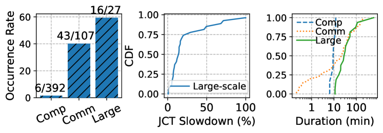
Figure 1: Left: Occurrence rate of fail-slows on computation and communication at node or link level and in large-scale training. Center: Impact of fail-slows on job completion time (JCT). Right: CDF of fail-slow duration.

In this paper, we propose Falcon, a system that rapidly identifies and reacts to computation and communication fail-slows without human intervention. Falcon achieves this through two subsystems, Falcon-Detect and Falcon-Mitigate. Falcon-Detect employs a non-intrusive, framework-agnostic mechanism for fail-slow detection. It keeps track of the training iteration time on each worker and identifies prolonged iterations using the Bayesian Online Change-point Detection (BOCD) algorithm [2]. It then initiates lightweight profiling on each worker to obtain a fine-grained execution profile for each parallelization group, without interrupting the ongoing training job. By analyzing these execution profiles, it narrows the search space to a few suspicious worker groups where fail-slows may reside. To pinpoint their exact locations within these groups, Falcon-Detect briefly pauses the training job and runs benchmarking tests to validate the GPU computation and link communication performance on each worker. Slow GPUs and links are then flagged as computation and communication fail-slows. Compared to full-job validation that involves benchmarking all GPUs and communication links, this design offers a lightweight solution.

Once fail-slows are detected, Falcon reacts with Falcon-Mitigate, using an efficient mitigation mechanism. As fail-slows are usually transient  (e.g., due to network congestion or CPU contention), simply handling them as fail-stops using checkpoint-and-restart is an overkill. In general, fail-slows can be tackled using four strategies: (S1) doing nothing, (S2) redistributing micro-batches across data parallel groups to alleviate the load on slow GPUs, (S3) adjusting the parallelization topology to move congested links to light-traffic groups, and (S4) treating fail-slows as fail-stops using checkpoint-and-restart. As we move from S1 to S4, the mitigation effectiveness improves, but the cost also increases. Therefore, the choice of optimal strategy depends on the duration (and severity) of the ongoing fail-slows, which cannot be known a priori. This problem resembles the classical ski-rental problem [19]. Drawing inspirations from its solution, we propose an effective ski-rental-like heuristic that starts with a low-cost strategy (S1) and progressively switches to a more effective, yet costly one if fail-slow persists and the current strategy proves ineffective. The mechanism falls back to checkpoint-and-restart as a last resort.

We have implemented Falcon with Falcon-Detect as a framework-independent detection system and Falcon-Mitigate as a plugin for Megatron-LM [42]. We use Falcon-Detect as the primary tool in our characterization study to identify computation and communication fail-slows for 499 sampling jobs submitted to the production cluster. Cross validation with human inspection shows that Falcon-Detect correctly diagnoses 498 jobs (99.8% accuracy), with less than 1% overhead. We further evaluate Falcon-Mitigate with manually injected fail-slows. Falcon-Mitigate reduces the slowdown from computation fail-slows by up to 82.9% and from communication fail-slows by up to 61.5%. Large-scale experiments involving a training job on 64 H800 GPUs demonstrate that Falcon mitigates the slowdown of fail-slows by 60.1%. Our contributions are summarized as follows:

1. We present the first comprehensive characterization study in a production cluster to understand the overall characteristics and performance impacts of fail-slow failures in hyperscale LM training.

2. We propose Falcon-Detect, a non-intrusive, framework-agnostic detection system that identifies computation and communication fail-slows at runtime.

3. We propose Falcon-Mitigate, a system that effectively addresses fail-slow failures through a novel multi-level straggler mitigation mechanism.

2 Background and Motivation

Hyperscale training can require thousands of petaFLOP/s of compute power, necessitating the use of high-performance computing (HPC) clusters [18, 8, 36, 29]. These HPC clusters typically consist of tens of thousands of GPUs interconnected through high-speed fabrics such as InfiniBand [35] and RoCE [20]. In this section, we briefly introduce the distributed training strategies on large HPC clusters and the inherent reliability issues during the training process.

Parallelism for Distributed Training. To efficiently train large models on HPC clusters, various parallelism strategies have been developed to partition and distribute models across GPUs and nodes.

1) Tensor Parallelism (TP). Tensor parallelism is a technique that partitions the computation of specific operators, such as MatMul or Attention, along non-batch axes [53, 42, 21]. This enables parallel computation of each partition across multiple devices. However, TP can incur significant communication costs due to the need for synchronization of each operator. Therefore, it is often confined to a single node to minimize latency and maximize throughput  [29, 18].

2) Data Parallelism (DP). Data parallelism involves creating multiple model replicas and distributing them across multiple GPUs [38, 42, 29]. In each iteration, the global data batch is split into mini-batches, allowing each model replica to handle a portion of the data concurrently. After each iteration, the gradients from all replicas are synchronized. Compared to TP, DP communication involves a moderate data transfer volume, which can occur either within a single node (intra-node) or across multiple nodes (inter-node).

3) Pipeline parallelism (PP). Pipeline parallelism partitions the model by placing different groups of layers, called stages, on separate GPUs [15, 53, 29]. It also divides the mini-batch into micro-batches, allowing for pipelined forward and backward passes across different nodes. PP incurs the smallest communication overhead among all three strategies. Therefore, PP stages are usually assigned to different nodes.

4) Hybrid parallelism. To maximize training efficiency, different parallelism strategies can be combined, allowing the model to be partitioned in multiple dimensions [29, 8, 18]. This technique, known as hybrid parallelism, have demonstrated the ability to train models with over a trillion parameters across thousands of GPUs, achieving high memory efficiency and near-linear scaling in terms of throughput as the cluster size expands [29, 18, 8].

Reliability Issues. Given the complex nature of distributed training and the sheer scale of resources involved, large model training presents significant reliability challenges, manifested as crash stoppage (fail-stop) and still-functioning but slow stragglers (fail-slow). Both types of failures stem from software or hardware problems, and their impacts are magnified in large-scale setup: a single failure component can crash or slow down the entire training process due to the frequent synchronization required in distributed training.

1) Fail-stop. Recent studies have focused on addressing fail-stop failures through effective fault tolerance mechanisms to minimize job downtime. These mechanisms either reduce the time spent on dumping and restoring model checkpoints [28, 48, 23] or perform redundant computations to minimize the need for costly checkpointing [45].

2) Fail-slow. Fail-slow, or straggler, is another a common problem in large-scale training. It can be caused by degraded hardware (such as network links or GPUs), buggy software, or contention from colocated jobs in a shared cluster. Compared to fail-stop issues, fail-slow problems are hard to detect [8], necessitating sophisticated performance analysis tools [18, 49]. Despite brief reports from recent studies [49, 8, 18], the overall characteristics of fail-slows remains largely unknown, which motivates our characterization study.

3 Characterization Study

In this section, we intend to answer the question, how do fail-slows manifest in large model training? We present a characterization study in a shared production cluster.

3.1 Cluster Setup and Methodology

Cluster Setup. Our production cluster consists of over 4,000 nodes and more than 10,000 heterogeneous GPUs, including approximately 1,800 NVIDIA H800 GPUs and 2,600 A100 GPUs. These nodes are connected through a high-performance network employing the popular spine-leaf architecture [36]. The network offers up to $4\times 200/400$ Gbps RoCE bandwidth for A100/H800 nodes. Within a node, GPUs are interconnected using NVSwitch [30]. The cluster runs diverse workloads, including:(1) large-scale model training jobs utilizing over 1,000 GPUs, (2) inference jobs encompassing both online inference and offline batch inference, (3) jobs for recommendation models, such as training embedding tables, and (4) short-running spot jobs for model debugging.

Methodology. As we are not allowed to directly instrument production workloads, we use two approaches to characterize fail-slows. (1) Online probing with repeated sampling. We repeatedly submitted identical small training jobs as spot workloads, which were randomly scheduled on available nodes across the cluster, often colocated with other production jobs. These training jobs are specially designed to act as probes, collecting key performance metrics and identifying computation and communication fail-slows at runtime using techniques developed in §4. By submitting a large number of these jobs, we can cover a sufficient number of nodes, effectively sampling the cluster for individual fail-slow events. (2) Offline inspection with collected traces. In addition to online probing, we collected a one-month trace containing numerous large-scale training jobs, each utilizing at least 512 GPUs. We manually inspected the trace to identify fail-slows.

3.2 How Computation Fail-Slows Manifest?

Sampling jobs. We start to characterize computation fail-slows occurred on individual nodes. We submitted 400 single-node training jobs to our cluster, of which 392 successfully completed without fail-stop errors. Each job trained a GPT2-11B model on one node using 4 H800 GPUs with a hybrid parallelism strategy of (2TP, 1DP, 2PP) to fully utilize GPU memory. The training framework used is Megatron-LM. Each job ran 10,000 iterations, taking 70 to 90 minutes. These sampling jobs were scheduled to run on approximately 500 out of 1,800 H800 GPUs in our cluster.

Frequency and impacts. As summarized in Table 1, six out of 392 sampling jobs experienced computation fail-slows. Of these, four jobs were slowed down due to CPU contention, and two due to GPU performance degradation. On average, these computation fail-slows persist for about 10 minutes, extending the job completion time (JCT) by 11.79%. To better understand the root causes of these issues, we next provide two case studies.

Category	Online Probing		Offline Inspection
	1-Node	4-Node	At Scale ($\geq 512$ GPUs)
No fail-slow	386	64	11
CPU Contention	4	1	0
GPU Degradation	2	0	0
Network Congestion	0	42	13
Multiple Issues	0	0	3
Total # Jobs	392	107	27
Avg. JCT Slowdown	11.79%	15.45%	34.59%

Table 1: Root causes and JCT slowdown of fail-slow issues in our characterization study.

Case-1: CPU contention. As shown in Figure 2 (upper-left), the job under study experienced two fail-slows at 22 and 55 minutes, resulting in a maximum performance drop of 21.6%. Correspondingly, the job measured simultaneous declines in SM utilization across all four GPUs during fail-slow periods (upper-right), suggesting GPU slowdown. To validate this, we paused the job and conducted a matrix computation to assess GPU performance upon fail-slow detection, but found no performance degradation. Further investigation revealed a surge in the number of high-CPU jobs coinciding with the fail-slow occurrence (bottom-left), leading to a decreased CPU satisfaction rate (bottom-right), increased CPU time, and ultimately, a reduction in throughput.

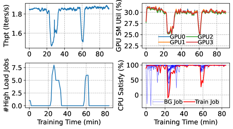
Figure 2: A case of a fail-slow job due to CPU contention. Upper-left: Training throughput. Upper-right: GPU SM utilization of the four GPUs used by this job. Bottom-left: The number of high-CPU jobs running on the same node. Bottom-right: CPU satisfaction rate of the training job (red) and other colocated jobs (blue).

Case-2: GPU performance degradation. Computation fail-slows can also be attributed to GPU performance degradation, often linked to frequency reduction due to thermal throttling. Figure 3 illustrates a case where the job under study experienced slowdown in the first 10 minutes (upper-left), resulting in under-utilization of all four GPUs (upper-right). Our profiling indicated that GPU0 was $20\%$ slower than others (bottom-left) and recorded an unusually high temperature of nearly $70^{\circ}C$. Notably, rising temperatures do not always lead to performance issues; this may indicate a hardware problem, with an occurrence rate of about 0.5%, consistent with ByteDance’s report [18].

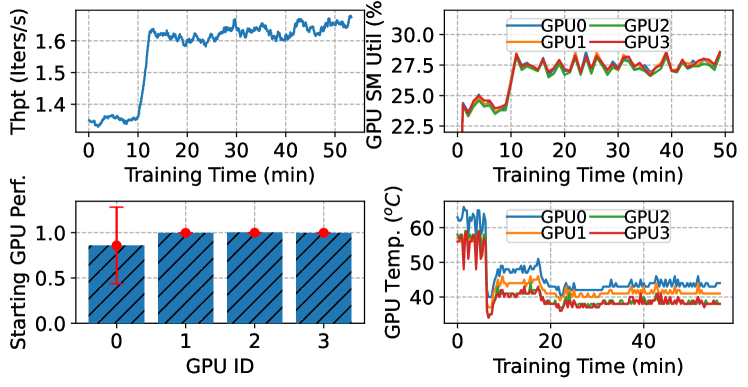
Figure 3: A case of a fail-slow job due to GPU performance degradation. Upper-left: Throughput of the training job. Upper-right: GPU SM utilization of the four GPUs used. Bottom-left: Normalized GPU performance during fail-slow. Bottom-right: Reported GPU temperature.

3.3 How Communication Fail-Slows Manifest?

Sampling jobs. To explore communication fail-slows, we submitted 120 four-node training jobs, of which 107 successfully completed without fail-stop. Each job utilized 8 A100 GPUs across 4 nodes to train a GPT2-7B model. The parallelism strategy employed was (2TP, 4DP, 1PP), where TP communications occurred intra-node via NVSwitch, and DP communications were inter-node through a 400 Gbps RoCE link. Each job executed 10,000 iterations, taking approximately 5 hours. These jobs were distributed among about 690 out of 2,600 A100 GPUs in our cluster.

Frequency and impacts. As detailed in Table 1, 43 out of 107 jobs experienced fail-slows. Among them, one job was slowed due to CPU contention, while the remaining 42 encountered network congestion. The average duration of these slowdowns was about 24 minutes, extending the average JCT by 15.45%.

Network congestion. Compared to computation slowdowns, network congestion emerges as a more significant factor contributing to performance degradation in multi-node training [37, 8], with a notably higher frequency. Figure 4 presents a case study on a sampling job that experienced two communication fail-slows at t=90 and t=265 minutes. The initial fail-slow resulted in throughput dipping from 0.57 to 0.41 iterations/s; shortly thereafter, at t=265, the second slowdown further reduced throughput to merely 0.31 iterations/s (Figure 4 (left)). We observed that the SM utilization across all 8 GPUs dropped simultaneously upon the onset of the fail-slow (right), despite the GPUs remaining healthy. Further investigation revealed a strong correlation between the surge of congestion notification packets (CNPs) reported by the NICs and the training slowdown (center).

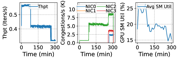
Figure 4: A case of fail-slow jobs caused by network congestion. Left: Training throughput. Center: The number of congestion notification packets ($\times 1000$) sent by NICs. Right: Average GPU SM utilization of the 8 GPUs used by the job.

Performance variation in communication. We further benchmarked communication performance variance among key components involved in training, including intra-GPU copies, inter-GPU communication via NVLink/NVSwitch (NVL), PCIe switch (PIX), and inter-node RDMA links. To evaluate their stability, we calculated the coefficient of variation (CoV) of their communication latency across these sampling jobs. As summarized in Table 2, both intra-GPU and NVL communication are stable, with CoVs below 0.02. In comparison, PIX shows more variability with a CoV of 0.09. Notably, inter-node RDMA exhibits the highest performance variance, with a CoV of 0.29, making it the least stable and most prone to fail-slow incidents.

Comm. Type	Intra-GPU		Intra-Node		Inter-Node
	A100	H800	NVL	PIX	RDMA
CoV	0.01	0.01	0.02	0.09	0.29

Table 2: Performance variation of key communication components. A higher CoV indicates less stability.

3.4 How Do Fail-Slows Manifest at Scale?

Limited by the small scale of each sampling job, online probing can only identify fail-slows occurred on individual nodes or links (§3.2 and §3.3). In large-scale training, a single slow GPU or congested link can delay the entire job, magnifying the impact of stragglers. To characterize fail-slows at a larger scale, we collected and manually examined a one-month trace containing 27 large-scale training jobs submitted to our cluster in July 2024, each utilizing 512 to 1024 GPUs.

Frequency and impacts. Among 27 jobs, 16 encountered fail-slows, delaying the average JCT by 34.59%. In particular, 20% of these jobs were delayed more than 50% (Figure 1, left). The mean fail-slow duration is 72 minutes, significantly longer than that measured in the small sampling jobs (Figure 1, right). Table 1 details the root causes of the encountered fail-slows, where 13 slow jobs were due to network congestion, while the remaining were attributed to both network and GPU degradation. We observed no CPU contention for these jobs as they ran exclusively on the training nodes.

Deep dive. Figure 5 illustrates the throughput of two 1024-GPU jobs, one for LLM training and the other for MoE model training. Both jobs experienced severe network congestion, leading to considerable throughput fluctuations, one at the initial stage (left) and the other throughout the training process (right). Worse still, at this scale, communication and computation fail-slows often compound, causing more damage to training. Figure 6 illustrates a case study. Throughout the training process, the observed throughput closely aligns with the GPU SM utilization. The first severe network congestion arose at t=62 minutes, slashing the training throughput by 80%. This degradation was further exacerbated by a GPU thermal throttling event occurred at around t=80 while the network congestion remains unabated, further reducing the throughput to just 10% of the normal performance. Subsequently, from t=120 onward, another severe network congestion persisted for about two hours, cutting the throughput by 85% again. This case highlights the compounding effects of multiple performance issues in large-scale training scenarios, which significantly undermines training efficiency.

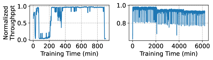
Figure 5: Two 1024-GPU jobs that failed slow due to network congestion. Left: An LLM training job. Right: An MoE training job with high variance and ladder-shaped fail-slow.

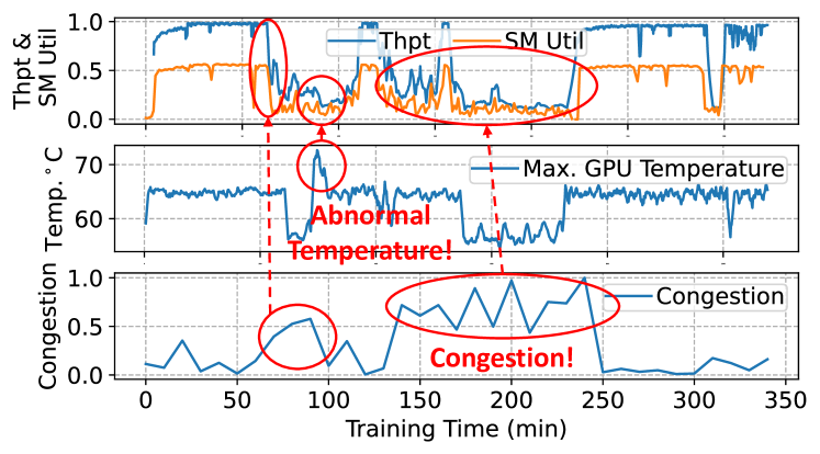
Figure 6: Case study of a 1024-GPU training job experiencing multiple performance issues, where fail-slow is caused by a compound of high GPU temperature and congested network.

Evidence from other companies. In addition to our study, straggler issues have been reported in Meta’s Llama training [8] and ByteDance’s MegaScale [18]. Our contacts with engineers from other companies bring attention to the similar fail-slow problems in LLM training, even on a single-tenant cluster with over 10,000 GPUs. The general consensus, as noted in [8, 18], is that fail-slows are hard to detect at scale.

3.5 Takeaways

Takeaway #1. Fail-slows are usually transient, primarily caused by degradation in computation and communication; the former typically stem from slow GPUs or CPU contention, while the latter are mainly due to network congestion.

Takeaway #2. Computation fail-slows tend to be short-lived and less frequent, leading to relatively minor performance degradation. In contrast, cross-node communication fail-slows are more common and tend to last longer, resulting in more significant training slowdowns.

Takeaway #3. As training scales up, the likelihood of simultaneously encountering multiple performance issues increases. The compounding effects of these issues can lead to significant training slowdowns, potentially exceeding 90%.

4 Falcon-Detect

Manually identifying fail-slows at scale, as we did in §3.4, is a daunting task. In this section, we design Falcon-Detect, a distributed monitoring and detection system for large-scale training that identifies performance issues in computation and communication at runtime. Falcon-Detect is designed to meet the following requirements.

R1: Non-intrusive and framework-independent. The detection system should not be bound to a specific training framework or require any modifications to the framework.

R2: Rapid and accurate. The system should rapidly identify the onset and resolution of fail-slow degradation while accurately locating the slow GPUs or communication links.

R3: Automated. The detection system should be fully automated, without human intervention.

R4: Lightweight. The system should introduce minimal inspection overhead to training, without costly full-job validations that typically require checkpoints and restarts.

4.1 System Overview

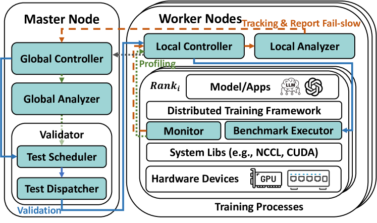
Figure 7: Architecture overview of Falcon-Detect.

Falcon-Detect is a distributed performance monitoring system deployed together with a large model training framework, such as DeepSpeed [39, 38] or Megatron-LM [42]. Figure 7 provides an architecture overview, with components introduced by Falcon-Detect highlighted in cyan. Falcon-Detect employs a master-worker architecture. On each worker node, multiple worker agents are co-deployed with the framework processes to monitor the training performance and report potential degradation to the master for further analysis and handling. Specifically, Falcon-Detect identifies fail-slows through a three-phase workflow: tracking, profiling, and validation.

1) Tracking. In this phase, each worker keeps track of the training iteration time for all training processes, called ranks, and detects slow iterations that indicate the onset of fail-slows. The worker reports these issues to the GlobalController, which transitions the system to the profiling phase.

2) Profiling. During this phase, the GlobalController instructs each worker to collect the detailed execution profiles of the ongoing training job. These log profiles are sent to the GlobalAnalyzer, which identifies suspicious worker groups that may contain fail-slows. The GlobalController then transitions the system to the validation phase.

3) Validation. In this final phase, the system initiates fail-slow validations within the suspicious worker groups to precisely locate slow GPUs or congested network links.

We next describe the detailed designs in the three phases.

4.2 Tracking

Falcon-Detect enters the tracking phase upon the execution of a training job, continuously monitoring its performance on each worker node. To maintain transparency to the training framework (R1), Falcon-Detect inserts a shim monitoring and benchmarking layer between the framework and the underlying system libraries, such as NCCL and CUDA (Figure 7). In this shim layer, a Monitor intercepts communication operations (i.e., NCCL function calls) from the training framework and logs their types and timestamps. This is done by hooking to NCCL functions using Linux’s LD_PRELOAD environment variable. The communication call logs, maintained in shared memory, are then retrieved by the node’s LocalAnalyzer, which infers the iteration time and detects slow iterations using two time series analysis techniques as follows.

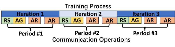
Figure 8: In iterative training, communication operations exhibit a clear periodic pattern, leading to recurring periods.

Iteration time analysis. Throughout iterations, various collective communication functions, such as ReduceScatter (RS), AllGather (AG), and AllReduce (AR), are invoked periodically. Figure 8 illustrates an example, where a training process exhibits a recurring period containing four communication calls. In practice, the number of communication calls involved in a recurring period and their patterns vary depending on the framework and the training model, which cannot be known due to the framework-agnostic requirement (R1).

To identify the recurring period from a call sequence, we employ a time series analysis approach based on auto-correlation function (ACF) [4]. Formally, given a call sequence $X=\{x_{1},x_{2},\ldots\}$, let $X_{t}$ be subsequence of $X$ containing $L$ elements starting from $x_{t}$. Let $k$ be the lag, which is a positive integer ranging from 1 to a predefined maximum. We evaluate the likelihood of $k$ being the recurring period of $X$ by calculating the corresponding ACF defined as follows:

$$\textstyle ACF(X)_{k}=\frac{Cov(X_{t},X_{t+k})}{Var(X_{t})}=\frac{\sum_{t=1}^{L-k}(X_{t}-\mu)(X_{t+k}-\mu)}{\sum_{t=1}^{L}(X_{t}-\mu)^{2}},\\$$

where $\mu$ is the mean of $X$. A higher value of $ACF(X)_{k}$ indicates a greater likelihood that $k$ is the recurring period of $X$. Thus, we can determine the recurring period of $X$ by identifying the first $k$ for which $ACF(X)_{k}$ exceeds a predefined threshold $M$ (set to 0.95 in our experiments), i.e.,

$$\textstyle\text{Period}=\text{arg}\min_{k}(ACF(X)_{k}\geq M).$$

Once the recurring period is identified, the iteration time derives by calculating the time difference between a communication operation and its occurrence in the previous period.

Slow iteration detection. To reliably identify slow iterations at runtime (R2), we propose to use the Bayesian online change-point detection (BOCD) algorithm [2] followed by a verification checking to differentiate between real fail-slow issues and normal performance jitters.

1) The BOCD algorithm. Bayesian online change-point detection is an efficient time series algorithm that finds change-points online in a dynamic sequence with linear time complexity. Feeding the algorithm the dynamic iteration time sequence, the identified change points usually correspond to the onset or relief of slow iterations. Specifically, the algorithm defines a run-length $r_{t}$ for each timestamp $t$ as follows:

$$r_{t}=\left\{\begin{array}[]{ll}0,&\text{if change-point at $t$,}\\ r_{t-1}+1,&\text{otherwise.}\\ \end{array}\right.$$

It then applies Bayesian inference to calculate the likelihood of $r_{t}=0$ (i.e., $t$ is a change-point) for each timestamp, and reports $t$ as a change-point if the likelihood exceeds a certain threshold (set to 0.9 in our experiments).

2) Change-point verification. While the BOCD algorithm identifies potential change-points, applying it directly to fail-slow detection results in numerous false positives, as many performance jitters may be misclassified as fail-slow incidents. To improve the detection accuracy (R2), we propose an additional verification step that compares the average iteration time before and after each identified change-point, treating it as a jitter if the performance difference is less than 10%.

In summary, the ACF-based iteration time analysis, combined with BOCD plus change-point verification, detects slow iterations reliably and rapidly (in linear time), thereby meeting requirement R2. Once slow iterations are detected on a worker node, the LocalAnalyzer reports to the master for further analysis and handling.

4.3 Profiling and Validation

Profiling. Experiencing slow iteration is a clear indicator of stragglers, which must be located rapidly. To avoid validating all components in distributed training (R4), which is prohibitively expensive at scale, Falcon-Detect narrows the search space by first identifying suspicious worker groups through a lightweight profiling process. Specifically, on each worker node, the LocalController instructs the Monitor to inject CUDA Events into each NCCL call to measure the execution time of each communication group. The results are then aggregated in the GlobalAnalyzer to identify degraded groups: a communication group that spent prolonged time in data transfer is likely experiencing fail-slow degradation, while groups that eagerly wait for data (i.e., idling) suggest healthy performance. In our implementation, communication groups with data transfer time longer than $1.1\times$ median value are classified as suspicious.

Lightweight training suspension. The profiling-identified suspicious groups need further validation to locate the precise degradation. As this requires running benchmark tests, the training job must be temporarily suspended. To avoid expensive checkpoint-and-restart (R4), we devise a lightweight training suspension mechanism. Since the Monitor hooks NCCL calls, it can pause the training by simultaneously “trapping” those calls into a wait loop and give control back to training processes once validation is done. This design enables validation to be performed in real time.

Validation. Upon training suspension, computation and communication benchmark tests are dispatched automatically to the suspicious worker groups to precisely locate the degraded components (R2 and R3).

1) Computation validation. To benchmark computation performance within a group, the TestDispatcher dispatches standard GEMM [31] tests to all GPUs in parallel to identify slow stragglers, if any.

2) Communication validation. Compared to slow GPUs, identifying the degraded network link is more challenging due to the complexity of collective communications performed with ring or tree topologies. To address this, we propose an automatic validation algorithm (R3) that divides the collective topology into non-overlapping peer-to-peer (P2P) operations. These operations can be executed efficiently in $O(1)$ time, regardless of the group size (R2), as illustrated in Figure 9.

Specifically, for a ring topology, the algorithm differentiates between even-rank and odd-rank rings. It divides even-rank rings into P2P send-receive operations that can be covered in two passes. In the first pass, data is transferred from even to adjacent odd ranks simultaneously (i.e., $0\rightarrow 1,2\rightarrow 3,\ldots$), while the second pass sends data from odd ranks to adjacent even ranks (Figure 9, left). For odd-rank rings, an additional pass is needed to accommodate the remaining link (Figure 9, center). For tree topology, the validation requires four passes (Figure 9, right). The first pass sends from left-child ranks at even levels to their parents, while the second pass sends from right-child ranks at even levels. The third and fourth passes reverse the roles of the senders, starting from odd levels. Since the transmission sizes are identical, slows link measures longer communication times and can be easily identified.

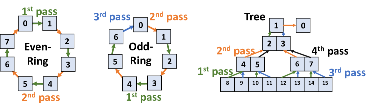
Figure 9: $O(1)$ validation of Ring and Tree communicators. Each cell is a rank, and the lines represent network links.

5 Falcon-Mitigate

In this section, we present Falcon-Mitigate, a system that effectively addresses fail-slows with a novel adaptive multi-level mitigation mechanism.

5.1 Design Space

Simply treating transient fail-slows as fail-stops by means of checkpoint-and-restart can do more harm than good, as dumping and restoring checkpoints for large models is time-consuming. In fact, dumping a GPT2-100B model takes nearly 100 minutes [48], even longer than the mean fail-slow duration in our cluster (§3). We explore the solution space and identify four strategies to address fail-slows.

(S1) Do nothing. This approach simply ignores fail-slow problems in the hope that the straggler components will soon be self-recovered. Many existing systems choose to do so due to the lack of an effective detection tool.

(S2) Adjust micro-batch distribution. This strategy is efficient in addressing computation fail-slows, which result in uneven processing speed among model replicas (i.e., DP groups). The strategy reacts by redistributing micro-batches across DP groups based on their processing speed, alleviating the load on slow GPUs and rebalancing the computation (§5.3).

(S3) Adjust parallelism topology. This strategy effectively mitigates both computation and communication stragglers by: 1) reassigning heavy-traffic communications to less congested links, thereby mitigating network congestion; and 2) consolidating multiple stragglers into the minimal number of PP stages, thus reducing their overall impact (§5.3).

(S4) Checkpoint-and-restart. As a last resort, the system performs checkpointing and restarts training on healthy nodes. While this approach effectively eliminates all fail-slows by replacing slow components, it incurs the highest overhead and may require significant human intervention.

We compare the four strategies in Table 3. As we move from S1 to S4, the mitigation effectiveness improves, but the action overhead also increases. Therefore, the optimal strategy varies depending on the severity and the duration of fail-slows. While the severity can be measured, the duration exhibits a large dynamic range, from tens of seconds to several hours (Figure 1, right), and cannot be predicted accurately.

Strategy	Effectiveness		Action Overhead
	Slow Comp.	Slow Comm.
S1: Ignore	No Effect	No Effect	No
S2: Adjust Microbatch	Mitigate	No Effect	Low
S3: Adjust Topology	Mitigate	Mitigate	Medium
S4: Ckpt-N-Restart	Eliminate	Eliminate	High

Table 3: Comparison of mitigation strategies in terms of effectiveness and overhead.

5.2 Adaptive Multi-Level Mitigation

We find that the mitigation planning problem resembles the classical ski-rental problem [19], which also involves balancing recurring ski-rental costs (akin to experiencing fail-slows) against a one-off ski-buying investment to avoid those costs (akin to taking mitigation action), all without prior knowledge of duration. The key insight from ski-rental is that it is optimal to initially rent a ski with the recurring rental cost and later fallback to ski buying when the accumulated rental cost equals the one-off investment.

Inspired by this, we design an adaptive multi-level fail-slow mitigation mechanism. It begins with a low-cost strategy (S1) and progressively switches to more effective—and hence more costly—strategies (S2 to S4) if fail-slow persists and the current approach proves ineffective. To determine the switch timing, the algorithm tracks the number of iterations affected by fail-slow and the resulting slowdowns to calculate an accumulated impact. It switches to the next strategy when this accumulated slowdown equals the action overhead of that strategy. Algorithm 1 formally describes this mechanism.

Algorithm 1 Adaptive Multi-level Fail-Slow Mitigation

1:function MitigationPlanner(event)

2:Input: The fail-slow event to handle.

3:    $\triangleright$ Find available strategies to mitigate this event.

4:    candidates $\leftarrow$ FindStrategies(event.root_cause)

5:    $\triangleright$ Sort the strategies by their overhead.

6:    candidates.sort(key=strategy.overhead)

7:    id $\leftarrow$ 0  $\triangleright$ Current mitigation strategy ID.

8:    while event.persist() do

9:        $\triangleright$ Get number of iterations that fails slow.

10:        slow_iters $\leftarrow$ event.get_slow_iters()

11:        $\triangleright$ Calculate the impact of fail-slow.

12:        slow_impact $\leftarrow$ slow_iters * ($t_{\text{slow}}-t_{\text{healthy}}$)

13:        $\triangleright$ Apply the current strategy and move forward.

14:        if slow_impact $\geq$ candidates[id].overhead then

15:           candidate_strategies[id].apply()

16:           id $\leftarrow$ id + 1

17:        end if

18:    end while

19:end function

5.3 Micro-batch and Parallelism Adjustment

We now describe the detailed design of the four strategies employed in the multi-level mitigation scheme. Since S1 and S4 are straightforward, we focus specifically on parallelism adjustment strategies S2 and S3.

Adjust micro-batch distribution. This strategy dynamically adjusts the number of micro-batches allocated to DP groups according to their computation performance, effectively mitigating computation fail-slows at a low cost. Specifically, DP partitions a large global batch into multiple micro-batches and distributes them evenly among all groups (i.e., model replicas) at initial. When a particular group experiences computation fail-slow, we rebalance the workload by reducing the number of micro-batches allocated to this group.

As shown in Equation (1), let $M$ represent the total number of micro-batches in a global batch, with $m_{i}$ micro-batches allocated to DP group $i$. The processing time for a micro-batch in DP group $i$ is denoted as $t_{i}$, which is profiled by Falcon-Detect (§4.3). Our goal is to minimize the processing time of the slowest DP group for all its micro-batches, which can be formulated as a quadratic programming problem that minimizes the variance in processing times across all DP groups:

$$\min\max_{i=1,\ldots,D}m_{i}t_{i}\Leftrightarrow\textstyle\min\sum_{i=1}^{D}(m_{i}t_{i}-\bar{m_{i}t_{i}})^{2},$$ (1)

$$\text{Subject to\quad}\textstyle m_{i}\in\mathbb{N}^{+}\text{ and }\sum_{i=1}^{D}m_{i}=M.$$

After this adjustment, although the workload may not be evenly distributed, the training loss can remain consistent by utilizing a weighted gradient aggregation method [5].

Overhead. The overhead from this adjustment mainly stems from the quadratic programming solver, such as cvxpy [7], and is typically low, lasting only a few seconds. Once the distribution is calculated, the adjustments can be applied immediately in the next iteration.

Adjust Topology. This strategy adjusts the network topology to reduce congestion and minimize PP stages affected by stragglers. This approach more effectively mitigates communication and computation fail-slow with moderate overhead.

Reassign congested links to light-traffic groups. In hybrid-parallel training, communication can be heavy between DP groups or light between adjacent PP stages [42, 29]. To mitigate fail-slow from network congestion, we can reassign congested links to light-traffic PP groups. For example, as shown in Figure 10, suppose the link between nodes 3 and 4 is congested and originally used for DP communication. By rearranging nodes 2 and 3, we can redirect the traffic from node 3 to 4 into light-traffic PP communication, effectively alleviating the impact of network congestion.

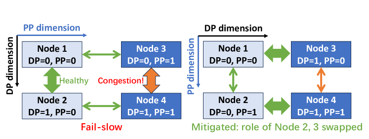
Figure 10: Topology adjustment to mitigate network congestion. After swapping Nodes 2 and 3, the congested link shifts from a heavy-traffic DP group to a lighter-traffic PP group.

Straggler consolidation. When multiple stragglers are present, consolidating them into one PP stage mitigates slowdown. Since workers within the same PP stage operates synchronously, the performance is determined by the slowest straggler, irrespective of the number of stragglers within this stage. In contrast, as shown in Figure 11, having stragglers scatter across multiple PP stages is sub-optimal. Therefore, in case of multiple stragglers, our topology adjustment aims to consolidate them into the minimal PP stages. To achieve this, we calculate the minimal number of PP stages needed to contain stragglers by $\lceil\#\text{Stragglers}/\text{\# GPUs per PP stage}\rceil$ and consolidate the stragglers accordingly. We also prefer to shift them to interior stages, as the first and last stages typically endure a higher load due to the pre- and post-processing modules (e.g., embedding layers) allocated to them.

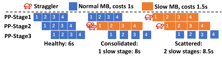
Figure 11: The number of straggling PP stages determines iteration time. With consolidated two stragglers in one stage, the iteration time is 8s, while it increases to 8.5s if the two stragglers are scattered across two stages.

Overhead. We perform topology adjustment in four steps: pausing ongoing training, temporally dumping parameters to swap into main memory, swapping parameters via RDMA, and restoring training. This process incurs moderate overhead, typically within one minute.

6 Implementation

We have implemented Falcon-Detect in approximately 5.5k LOC. The Monitor and BenchmarkExecutor are developed in C++ and CUDA, hooking NCCL functions via LD_PRELOAD. Other components are written in Python, which communicate with the C++ modules through shared memory and Redis [41] for intra-node and inter-node communications, respectively. Additionally, Falcon-Mitigate is implemented in 1.5k LOC, including a planner module and several strategy modules. The planner receives slow component IDs from Redis and generates adjustment plans. These plans are then executed by the strategy modules, which are implemented as lightweight plugins for Megatron [42].

7 Evaluation

In this section, we evaluate Falcon-Detect and Falcon-Mitigate to answer the following questions:

1. How accurately does Falcon-Detect estimate iteration time and identify fail-slow incidents across various models and parallelism configurations? (§7.2)

2. Is Falcon-Mitigate effective in alleviating various fail-slow conditions across different root causes and parallelism configurations? (§7.3)

3. What is the overhead associated with Falcon-Detect and the various mitigation strategies implemented in Falcon-Mitigate? (§7.4)

4. How effective is Falcon in enhancing training efficiency and mitigating the impact of fail-slow incidents in large-scale real-world training scenarios? (§7.5)

7.1 Experiment Setup

Testbed configuration. We conduct our evaluation on a high-performance cluster comprising 55 nodes, each equipped with 8 NVIDIA H800 GPUs connected via NVSwitch. The nodes are interconnected through a 400Gbps InfiniBand network in a spine-leaf topology, ensuring symmetric inter-node bandwidth. Our tests utilize Megatron-LM [42], a large-scale distributed training framework built on PyTorch [3], to train a set of GPT-2 models in various sizes and parallel strategies. The testbed runs CUDA version 12.2 and NCCL version 2.18.1.

Fail-slow injection. Since fail-slow incidents occur unpredictably, we evaluate the effectiveness of our mitigation system using deterministic manually injected fail-slows. To simulate computational fail-slows, we employ the nvidia-smi -lgc command to lock the GPU SM frequency, mimicking the GPU performance degradation. To inject communication fail-slows, we initiate side-channel communication jobs that create network bandwidth contention, thereby reducing the available bandwidths on specific network links.

7.2 How Accurate Is Detection?

Iteration time estimation. We first evaluate how accurately Falcon-Detect estimates the iteration time across various hybrid-parallel strategies, as an accurate estimation is the foundation of fail-slow detection. We deploy GPT2-7B training jobs using different parallel strategies on 1, 2, and 4 nodes. As illustrated in Figure 12, in single-node experiments with 4 GPUs, the relative error remains below 1.2% compared to the ground truth iteration time, regardless of the parallel strategies employed. In a 2-node experiment with a (2TP, 2DP, 2PP) configuration, the error is 0.7%, while in a 4-node test with a (2TP, 4DP) setup, it remains highly accurate at just 0.1% relative error. These experiments highlight the accuracy of our ACF-based iteration time estimation.

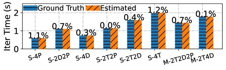
Figure 12: Accuracy of iteration time estimation in single-node ($S$) and multi-node ($M$) settings. The notation $xTyDzP$ specifies the TP size $x$, DP size $y$, and PP size $z$.

Fail-slow detection. We assess the effectiveness of our BOCD plus verification algorithm (BOCD+V) in detecting computation and communication fail-slows. The baseline methods are slide-window and classical BOCD; the former reports a fail-slow if there’s a >10% performance change in the sliding window from the current median, while the latter lacks verification. Using traces from our characterization study, we assess their accuracy against human-labeled ground truth. As shown in Table 4, BOCD+V achieves perfect 100% accuracy with 0% False-Positive Rate (FPR) and 0% False-Negative Rate (FNR) in detecting computation fail-slow. In the case of communication fail-slow (as illustrated in Table 5), BOCD+V attains 99.1% accuracy, 0% FPR, and only 2.3% FNR. The FNR primarily dues to a rare case containing consecutive <10% degradations. The original BOCD has a lower FNR by reporting all suspicious change-points but suffers from a high FPR. Similarly, the slide-window method is less accurate, as it misses many fail-slow cases and shows a higher FNR.

Algorithm	Accuracy$\uparrow$ (%)	FPR$\downarrow$ (%)	FNR$\downarrow$ (%)
SlideWindow	99.5(390/392)	0.0(0/386)	25.0(2/8)
BOCD	77.8(305/392)	18.39(87/473)	0.0(0/6)
BOCD+V	100.0(392/392)	0.0(0/386)	0.0(0/6)

Table 4: Comparison across detection algorithms for computation fail-slows.

Algorithm	Accuracy$\uparrow$ (%)	FPR$\downarrow$ (%)	FNR$\downarrow$ (%)
SlideWindow	93.5(100/107)	1.5(1/65)	12.2(6/49)
BOCD	69.2(74/107)	34.0(33/97)	0.00(0/43)
BOCD+V	99.1(106/107)	0.00(0/64)	2.3(1/44)

Table 5: Comparison across detection algorithms for communication fail-slows.

7.3 How Effective Is Mitigation?

Effectiveness of micro-batch distribution adjustment (S2). To evaluate the effectiveness of strategy S2 in mitigating computation fail-slows, we deploy a single-node training with 8 GPUs. We inject weak (W), medium (M), and severe (S) computation fail-slows to a single GPU into single-node training jobs with 2, 4, and 8 DP groups, as illustrated in Figure 13. Our approach reduces the slowdown by 55.3%, 77.8%, and 64.9% for 2, 4, and 8 DP groups, achieving reductions of up to 82.9%. This strategy proves effective across various setups and fail-slow severity since it consistently ensures a dynamic load balance across all DP groups.

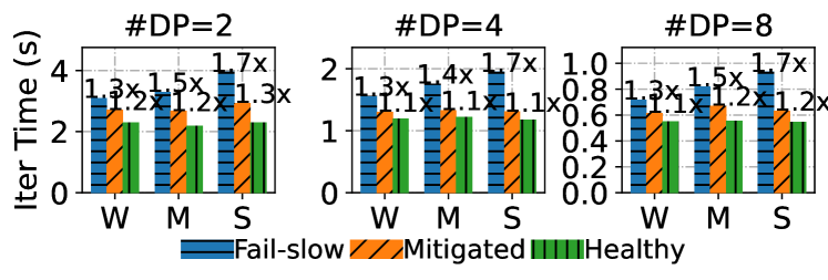
Figure 13: Effectiveness of micro-batch adjustment strategy of mitigating various fail-slow severities and DP settings.

As shown in Figure 14, we evaluate S2’s effectiveness when multiple DP groups experience fail-slow. In a 4-DP training job, we inject slow computation into 0 to 4 of these groups. S2 achieves its best performance with only one slow DP group, reducing slowdown by 79.7% ($1.9\times$ to $1.2\times$). Our findings reveal that while multiple slow DP groups do not further increase iteration time, the room for mitigation decreases as the number of degraded DP groups rises. This occurs because when multiple DP groups are affected, total computational power decreases, limiting adjustment flexibility, and there is no room for adjustment if all four groups are degraded.

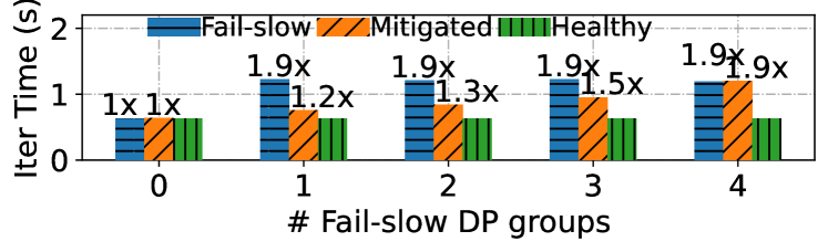
Figure 14: Effectiveness of micro-batch adjustment strategy of mitigating various number of fail-slow DP groups.

Effectiveness of topology adjustment (S3). We evaluate the effectiveness of strategy S3 by a 2-node experiment with 16 GPUs. As shown in Figure 15, we inject communication fail-slow into training jobs with 4 or 8 PP stages. The results reveal a reduction in the average slowdown by 53.7% and 24.8% for 4 and 8 PP stages, respectively, with a maximum of 61.5% (PP=4, weak congestion). The strategy is more effective with 4-stage PP due to the increased bubble rate and longer idle times associated with the longer pipeline in the 8-stage setup, which ultimately understates the effectiveness.

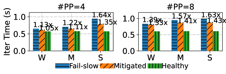
Figure 15: Effectiveness of topology adjustment strategy of mitigating various fail-slow severity and PP settings.

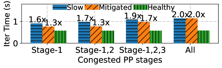
Figure 16: Effectiveness of straggler consolidation of mitigating multiple fail-slow PP stages.

To evaluate the effectiveness of straggler consolidation in topology adjustment, we conduct an experiment with 16 GPUs using (4DP, 4PP) setup. As shown in Figure 16, congestion in one link affecting a pair of GPUs in PP stage-1 raises iteration time to $1.6\times$, which can be mitigated to $1.3\times$. Injecting two slow links affecting two stages slows down iteration time to $1.7\times$, but can also be mitigated to $1.3\times$ through consolidation into only one PP stage. With three congested links affecting 6 GPUs, mitigation reduces iteration time from $1.9\times$ to $1.7\times$, since one stage contains only four GPUs and six stragglers must occur across two PP stages. If all links are slow, there is no room for adjustment.

Case study: compound of slow comp. and comm. We evaluate Falcon-Mitigate in a more complex scenario involving a combination of slow computation and communication, mirroring the case presented in our characterization (§ 3.4). As shown in Figure 17, throughput drops from 1.7 to 1.0 iterations/s due to slow communication at t=30. After applying topology adjustments, throughput improves to 1.3 iterations/s. Within this period, the computation performance of one GPU degrades at t=200, causing throughput to further decline to 0.5 iterations/s, which is subsequently mitigated to 0.9 iterations/s. By t=450, the impact of the fail-slow surpasses the restart threshold, triggering a checkpoint-restart, with training resuming at 1.7 iterations/s. This experiment demonstrates the effectiveness of Falcon-Mitigate’s multi-level mitigation algorithm in handling fail-slow issues arising from mixed performance issues.

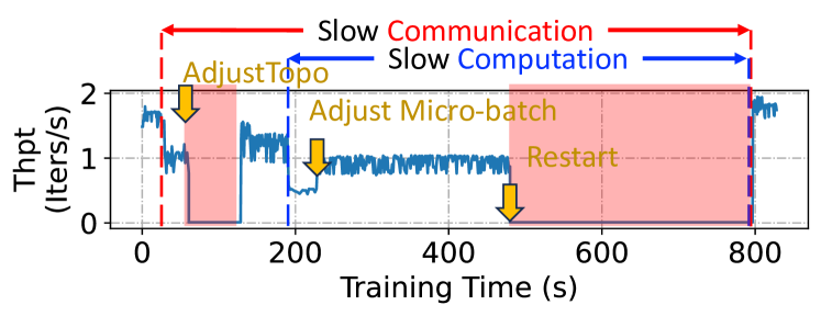
Figure 17: Effectiveness of Falcon-Mitigate in a case of both computation and communication fail slow.

7.4 How Large Is the Overhead?

In this section, we evaluate the detection and mitigation overhead introduced by Falcon.

Detector overhead. To assess the overhead introduced by Falcon-Detect, we conducted training under the same hybrid-parallel settings as in § 7.2. As shown in Figure 18, the average overhead is only 0.39%, with a maximum of 1.1% compared to training without the detector. In some instances, the iteration time with the detector is even lower than without it—reflecting training variability, as indicated by the 0.0% in green. These results demonstrate that the overhead of Falcon-Detect is negligible.

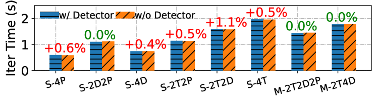
Figure 18: Overhead introduced by Falcon-Detect across various parallel strategies.

Micro-batch adjustment overhead. We evaluate the overhead for adjusting the micro-batch distribution, which primarily arises from solving Equation 1. As shown in Table 6, although this overhead increases exponentially with the number of DP groups, it remains around 30 seconds even with 512 DP groups, showing its efficiency for hyperscale training.

# DPs	16	32	64	128	256	512
Time(s)	0.01	0.01	0.01	0.11	6.78	35.93

Table 6: Time to find the optimal micro-batch distribution.

Topology adjustment overhead. We evaluate the topology adjustment overhead across various GPU memory utilization levels. As shown in Figure 19, this memory-based approach reduces pause time by up to $6.72\times$ compared to the disk-based baseline, primarily by eliminating checkpoint dumping and loading times. The performance gains are more pronounced with higher GPU memory utilization, as the disk operation times increase significantly for large I/O sizes.

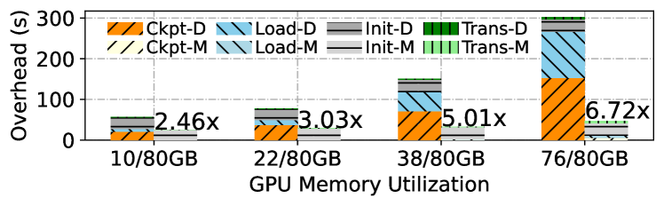
Figure 19: Breakdown of topology adjustment overhead. M denotes memory dump and load (our method), while D represents disk-based as the baseline method.

7.5 How Does Falcon Perform at Scale?

To evaluate Falcon’s performance in large-scale training, we conduct a hybrid-parallel training of GPT2-13B on 64 GPUs using a (16DP, 4PP) configuration. We manually inject two communication and eight computation fail-slows of varying severity, as illustrated in Figure 20, bottom. This training job is executed twice with the same fail-slow trace: once with Falcon and once without it for comparison.

As shown in the top of Figure 20, when the computation stragglers are present, training throughput without Falcon drops significantly throughout the slow periods, while it is quickly recovered to near-optimal levels with Falcon in place, showing the effectiveness of our micro-batch adjustment strategy. During communication slowdowns, we initiate brief pauses (at t=600 and t=2100) for topology adjustments, each lasting under a minute, much faster than a typical checkpoint-and-restart that takes tens of minutes. Notably, the compound of computation and communication issues could reduce performance by nearly 50%, but with Falcon, this decline is mitigated to only 25%.

We present the average performance from both runs in Table 7. Without fail-slows, the average training throughput is about 17.1 iterations/min. When fail-slows are introduced but not mitigated, the average throughput drops to 14.8 iterations/min. However, integrating Falcon allows throughput to recover to 16.2 iterations/min under the same conditions. These results demonstrate that Falcon reduces slowdown by 60.1%, improving end-to-end job completion time from $1.15\times$ optimal to $1.05\times$ optimal.

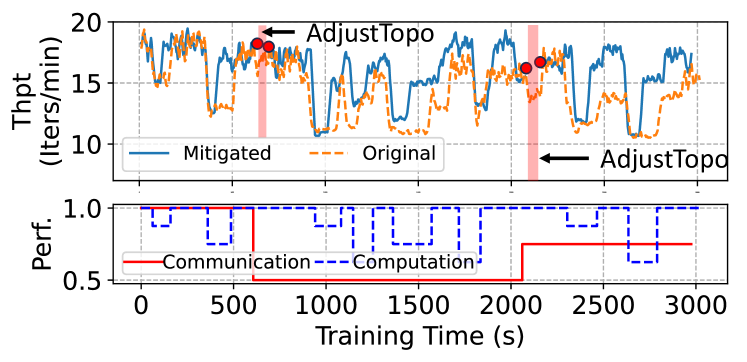
Figure 20: Evaluation of Falcon for a 64-GPU training with mixed computation and communication fail-slows.

Healthy Thpt.	Fail-slow Thpt.	Mitigated Thpt.	Slowdown
17.1 Iters/min	14.8 Iters/min	16.2 Iters/min	-60.1%

Table 7: Effectiveness of Falcon, which reduces the impact of fail-slow by 60.1%.

8 Related Work

Reliability issues in training. Several studies address the fail-stop issue using checkpoint-based methods [28, 48, 23], re-computation approaches [45], and elastic frameworks [16, 54]. In contrast, while fail-slow have been acknowledged in various reports [8, 18], the only existing detection solution, SuperBench [49], requires checkpoint-and-restart for benchmarking, leading to prohibitively high overhead. Additionally, to the best of our knowledge, there are no fail-slow mitigation systems available currently.

Fail-slow in other fields. The fail-slow issue also exists in cloud services [14, 6, 10, 11, 13, 24], operating systems [51], and storage [12, 25], but presents unique challenges in large-scale training. In cloud and OS, the main issue is identifying the source of gradually propagating fail-slow [10, 11]. In contrast, large-scale training is synchronous, one slow component can immediately propagate to the entire cluster. Handling storage fail-slow is simpler since disks operate independently [25]. Additionally, replacing degraded components in these fields is often inexpensive and doesn’t impact the entire system.

Heterogeneous DL training. Several researches focus on efficient parallel training on heterogeneous hardware with various performance [46, 17, 5, 50, 33, 27, 53, 26]. However, mitigating fail-slow presents distinct challenges. Heterogeneous training is static, where performance does not fluctuate over time, thus allowing for higher-cost parallel strategy searches at initial [46, 53]. In contrast, fail-slow handling must be dynamic, precluding those high-cost searches.

9 Conclusion

In this paper, we systematically studied the fail-slow issue in large-scale hybrid-parallel training through comprehensive characterization. Building on these insights, we propose Falcon, a framework that swiftly identifies fail-slowed compute or communication components and effectively mitigates them using a novel multi-level mechanism, all without human intervention. Falcon achieves over 99% accuracy in detecting fail-slows and reduces slowdown by 60.1% in large-scale training.

Appendix

9.1 Formulation of BOCD Algorithm

The run-length (RL) $r_{t}$ indicates if there is a change-point at time $t$, which is defined as

$$r_{t}=\begin{cases}0,\quad\text{if change-point at time t,},\\ r_{t-1}+1,\quad\text{otherwise.}\end{cases}$$ (2)

Given a time series $X=\{x_{i}\}_{i=1}^{T}$, the probability of $x_{t+1}$ given $x_{1:t}$ is

$$\Pr(x_{t+1}|x_{1:t}) =\sum_{r_{t}}\Pr(r_{t},x_{t+1}|x_{1:t})$$ (3)

$$=\sum_{r_{t}}\Pr(x_{t+1}|r_{t},x_{l})\Pr(r_{t}|x_{1:t})$$

$$=\sum_{l=0}^{t}\Pr(x_{t+1}|r_{t}=l,x_{t-l:t})\Pr(r_{t}=l|x_{1:t}),$$

where $x_{l}$ is to denote all observations associated with $r_{t}=l$. The first term $\Pr(x_{t+1}|r_{t},x_{l})$ is called Underlying Probabilistic Model (UPM) predictive, while $\Pr(r_{t}|x_{1:t})$ is called RL posterior.

The RL posterior can be calculated by

$$\Pr(r_{t}|x_{1:t})=\frac{\Pr(r_{t},x_{1:t})}{\sum_{r_{t}^{\prime}}\Pr(r_{t}^{\prime},x_{1:t})}.$$ (4)

Therefore, the joint probability $\Pr(r_{t},x_{1:t})$ is

$$\Pr(r_{t},x_{1:t}) =\sum_{r_{t-1}}\Pr(r_{t},r_{t-1},x_{1:t-1},x_{t})$$ (5)

$$=\sum_{r_{t-1}}\Pr(r_{t},x_{t}|r_{t-1},x_{1:t-1})\Pr(r_{t-1},x_{1:t-1})$$

$$=\sum_{r_{t-1}}\Pr(x_{t}|r_{t},x_{l})\Pr(r_{t}|r_{t-1})\Pr(r_{t-1},x_{1:t-1}),$$

where $\Pr(x_{t}|r_{t},x_{l})$ is the UPM predictive, $\Pr(r_{t}|r_{t-1})$ is called change-point prior reflecting the prior knowledge of change-points (e.g., expectation of fail-slow interval), and $\Pr(r_{t-1},x_{1:t-1})$ is recursively computed in the previous step.

9.2 Communication Volumes in Hybrid-Parallel Training

Parameter size of transformer models. Suppose the model has $L$ layers, hidden size is $h$, number of heads is $n_{h}$, attention head dimension $d$, vocabulary size is $v$, max context length is $n_{ctx}$. Then the number of parameters $N$ of the model is

$$N =N_{we}+N_{pe}+N_{attn}+N_{ffn}$$ (6)

$$=vh+n_{ctx}h+4hn_{h}dL+L(8h^{2}+5h)$$

$$=h\left(v+n_{ctx}+L\left(4dn_{h}+8h+5\right)\right)\approx 12Lh^{2}.$$

Communication volumes. Suppose the model is distributed to $T$ TP groups, $D$ DP groups, and $P$ PP stages, then the number of parameters per GPU is

$$N_{GPU}=\frac{N}{TP}.$$ (7)

Assume the input micro-batch size is $b$, with $m$ micro-batches, then communication volume for tensor parallel per iteration is

$$Comm_{TP}=8bmn_{ctx}h\frac{L(T-1)}{PT}.$$ (8)

, which has the largest volume, but it is usually intra-node communication.

The communication volume per iteration for data parallel is the total size of gradients, which is proportional to number of parameters per GPU

$$Comm_{DP}=kN_{GPU}\approx\frac{12kLh^{2}}{PT}.$$ (9)

The communication of pipeline parallelism is the activation of each stage, hence its volume per iteration is

$$Comm_{PP}=mbn_{ctx}h.$$ (10)

Therefore, $Comm_{DP}\gg Comm_{PP}$ in training since $Comm_{DP}$ is $\Theta(h^{2})$, while $Comm_{PP}$ is $\Theta(h)$, with $h$ as the dominant factor. Therefore, adjusting topology can significantly reduce communication volume on congested network links.

References

- [1] Josh Achiam, Steven Adler, Sandhini Agarwal, Lama Ahmad, Ilge Akkaya, Florencia Leoni Aleman, Diogo Almeida, Janko Altenschmidt, Sam Altman, Shyamal Anadkat, et al. Gpt-4 technical report. arXiv preprint arXiv:2303.08774, 2023.
- [2] Diego Agudelo-España, Sebastian Gomez-Gonzalez, Stefan Bauer, Bernhard Schölkopf, and Jan Peters. Bayesian online prediction of change points. In Conference on Uncertainty in Artificial Intelligence, pages 320–329. PMLR, 2020.
- [3] Jason Ansel, Edward Yang, Horace He, Natalia Gimelshein, Animesh Jain, Michael Voznesensky, Bin Bao, Peter Bell, David Berard, Evgeni Burovski, et al. Pytorch 2: Faster machine learning through dynamic python bytecode transformation and graph compilation. In Proceedings of the 29th ACM International Conference on Architectural Support for Programming Languages and Operating Systems, Volume 2, pages 929–947, 2024.
- [4] Christopher Chatfield. The analysis of time series: theory and practice. Springer, 2013.
- [5] Chen Chen, Qizhen Weng, Wei Wang, Baochun Li, and Bo Li. Semi-dynamic load balancing: Efficient distributed learning in non-dedicated environments. In Proceedings of the 11th ACM Symposium on Cloud Computing, pages 431–446, 2020.
- [6] Mike Chow, Yang Wang, William Wang, Ayichew Hailu, Rohan Bopardikar, Bin Zhang, Jialiang Qu, David Meisner, Santosh Sonawane, Yunqi Zhang, et al. ServiceLab: Preventing tiny performance regressions at hyperscale through Pre-Production testing. In 18th USENIX Symposium on Operating Systems Design and Implementation (OSDI 24), pages 545–562, 2024.
- [7] Steven Diamond and Stephen Boyd. CVXPY: A Python-embedded modeling language for convex optimization. Journal of Machine Learning Research, 17(83):1–5, 2016.
- [8] Abhimanyu Dubey, Abhinav Jauhri, Abhinav Pandey, Abhishek Kadian, Ahmad Al-Dahle, Aiesha Letman, Akhil Mathur, Alan Schelten, Amy Yang, Angela Fan, et al. The llama 3 herd of models. arXiv preprint arXiv:2407.21783, 2024.
- [9] William Fedus, Barret Zoph, and Noam Shazeer. Switch transformers: Scaling to trillion parameter models with simple and efficient sparsity. Journal of Machine Learning Research, 23(120):1–39, 2022.
- [10] Yu Gan, Mingyu Liang, Sundar Dev, David Lo, and Christina Delimitrou. Sage: Leveraging ml to diagnose unpredictable performance in cloud microservices. arXiv preprint arXiv:2112.06263, 2021.
- [11] Yu Gan, Yanqi Zhang, Kelvin Hu, Dailun Cheng, Yuan He, Meghna Pancholi, and Christina Delimitrou. Seer: Leveraging big data to navigate the complexity of performance debugging in cloud microservices. In Proceedings of the twenty-fourth international conference on architectural support for programming languages and operating systems, pages 19–33, 2019.
- [12] Haryadi S Gunawi, Riza O Suminto, Russell Sears, Casey Golliher, Swaminathan Sundararaman, Xing Lin, Tim Emami, Weiguang Sheng, Nematollah Bidokhti, Caitie McCaffrey, et al. Fail-slow at scale: Evidence of hardware performance faults in large production systems. ACM Transactions on Storage (TOS), 14(3):1–26, 2018.
- [13] Peng Huang, Chuanxiong Guo, Jacob R Lorch, Lidong Zhou, and Yingnong Dang. Capturing and enhancing in situ system observability for failure detection. In 13th USENIX Symposium on Operating Systems Design and Implementation (OSDI 18), pages 1–16, 2018.
- [14] Peng Huang, Chuanxiong Guo, Lidong Zhou, Jacob R Lorch, Yingnong Dang, Murali Chintalapati, and Randolph Yao. Gray failure: The achilles’ heel of cloud-scale systems. In Proceedings of the 16th Workshop on Hot Topics in Operating Systems, pages 150–155, 2017.
- [15] Yanping Huang, Youlong Cheng, Ankur Bapna, Orhan Firat, Dehao Chen, Mia Chen, HyoukJoong Lee, Jiquan Ngiam, Quoc V Le, Yonghui Wu, et al. Gpipe: Efficient training of giant neural networks using pipeline parallelism. In NeurIPS, 2019.
- [16] Insu Jang, Zhenning Yang, Zhen Zhang, Xin Jin, and Mosharaf Chowdhury. Oobleck: Resilient distributed training of large models using pipeline templates. In Proceedings of the 29th Symposium on Operating Systems Principles, pages 382–395, 2023.
- [17] Xianyan Jia, Le Jiang, Ang Wang, Wencong Xiao, Ziji Shi, Jie Zhang, Xinyuan Li, Langshi Chen, Yong Li, Zhen Zheng, et al. Whale: Efficient giant model training over heterogeneous GPUs. In 2022 USENIX Annual Technical Conference (USENIX ATC 22), pages 673–688, 2022.
- [18] Ziheng Jiang, Haibin Lin, Yinmin Zhong, Qi Huang, Yangrui Chen, Zhi Zhang, Yanghua Peng, Xiang Li, Cong Xie, Shibiao Nong, et al. MegaScale: Scaling large language model training to more than 10,000 GPUs. In 21st USENIX Symposium on Networked Systems Design and Implementation (NSDI 24), pages 745–760, 2024.
- [19] Anna R Karlin, Claire Kenyon, and Dana Randall. Dynamic tcp acknowledgement and other stories about e/(e-1). In Proceedings of the thirty-third annual ACM symposium on Theory of computing, pages 502–509, 2001.
- [20] Gurkirat Kaur and Manju Bala. Rdma over converged ethernet: A review. International Journal of Advances in Engineering & Technology, 6(4):1890, 2013.
- [21] Vijay Anand Korthikanti, Jared Casper, Sangkug Lym, Lawrence McAfee, Michael Andersch, Mohammad Shoeybi, and Bryan Catanzaro. Reducing activation recomputation in large transformer models. In MLSys, 2023.
- [22] Dmitry Lepikhin, HyoukJoong Lee, Yuanzhong Xu, Dehao Chen, Orhan Firat, Yanping Huang, Maxim Krikun, Noam Shazeer, and Zhifeng Chen. Gshard: Scaling giant models with conditional computation and automatic sharding. arXiv preprint arXiv:2006.16668, 2020.
- [23] Yuanhao Li, Tianyuan Wu, Guancheng Li, Yanjie Song, and Shu Yin. Portus: Efficient dnn checkpointing to persistent memory with zero-copy. In 2024 IEEE 44th International Conference on Distributed Computing Systems (ICDCS), pages 59–70. IEEE, 2024.
- [24] Chang Lou, Peng Huang, and Scott Smith. Understanding, detecting and localizing partial failures in large system software. In 17th USENIX Symposium on Networked Systems Design and Implementation (NSDI 20), pages 559–574, 2020.
- [25] Ruiming Lu, Erci Xu, Yiming Zhang, Fengyi Zhu, Zhaosheng Zhu, Mengtian Wang, Zongpeng Zhu, Guangtao Xue, Jiwu Shu, Minglu Li, et al. Perseus: A Fail-Slow detection framework for cloud storage systems. In 21st USENIX Conference on File and Storage Technologies (FAST 23), pages 49–64, 2023.
- [26] Yixuan Mei, Yonghao Zhuang, Xupeng Miao, Juncheng Yang, Zhihao Jia, and Rashmi Vinayak. Helix: Distributed serving of large language models via max-flow on heterogeneous gpus. arXiv preprint arXiv:2406.01566, 2024.
- [27] Xupeng Miao, Yining Shi, Zhi Yang, Bin Cui, and Zhihao Jia. Sdpipe: A semi-decentralized framework for heterogeneity-aware pipeline-parallel training. Proceedings of the VLDB Endowment, 16(9):2354–2363, 2023.
- [28] Jayashree Mohan, Amar Phanishayee, and Vijay Chidambaram. CheckFreq: Frequent,Fine-GrainedDNN checkpointing. In 19th USENIX Conference on File and Storage Technologies (FAST 21), pages 203–216, 2021.
- [29] Deepak Narayanan, Mohammad Shoeybi, Jared Casper, Patrick LeGresley, Mostofa Patwary, Vijay Korthikanti, Dmitri Vainbrand, Prethvi Kashinkunti, Julie Bernauer, Bryan Catanzaro, et al. Efficient large-scale language model training on gpu clusters using megatron-lm. In Proceedings of the International Conference for High Performance Computing, Networking, Storage and Analysis, pages 1–15, 2021.
- [30] NVIDIA Corporation. Fabric manager for nvidia nvswitch systems, 2023. Accessed: 2024-09-04.
- [31] NVIDIA Corporation. Matrix multiplication background user’s guide, 2024. Accessed: 2024-09-17.
- [32] OpenAI. Openai sora, 2024. Accessed: 2024-09-13.
- [33] Jay H Park, Gyeongchan Yun, M Yi Chang, Nguyen T Nguyen, Seungmin Lee, Jaesik Choi, Sam H Noh, and Young-ri Choi. HetPipe: Enabling large DNN training on (whimpy) heterogeneous GPU clusters through integration of pipelined model parallelism and data parallelism. In 2020 USENIX Annual Technical Conference (USENIX ATC 20), pages 307–321, 2020.
- [34] William Peebles and Saining Xie. Scalable diffusion models with transformers. In Proceedings of the IEEE/CVF International Conference on Computer Vision, pages 4195–4205, 2023.
- [35] Gregory F Pfister. An introduction to the infiniband architecture. High performance mass storage and parallel I/O, 42(617-632):10, 2001.
- [36] Kun Qian, Yongqing Xi, Jiamin Cao, Jiaqi Gao, Yichi Xu, Yu Guan, Binzhang Fu, Xuemei Shi, Fangbo Zhu, Rui Miao, et al. Alibaba hpn: A data center network for large language model training. In Proceedings of the ACM SIGCOMM 2024 Conference, pages 691–706, 2024.
- [37] Sudarsanan Rajasekaran, Manya Ghobadi, and Aditya Akella. CASSINI:Network-Aware job scheduling in machine learning clusters. In 21st USENIX Symposium on Networked Systems Design and Implementation (NSDI 24), pages 1403–1420, 2024.
- [38] Samyam Rajbhandari, Jeff Rasley, Olatunji Ruwase, and Yuxiong He. Zero: Memory optimizations toward training trillion parameter models. In IEEE/ACM SC, 2020.
- [39] Jeff Rasley, Samyam Rajbhandari, Olatunji Ruwase, and Yuxiong He. Deepspeed: System optimizations enable training deep learning models with over 100 billion parameters. In Proceedings of the 26th ACM SIGKDD International Conference on Knowledge Discovery & Data Mining, pages 3505–3506, 2020.
- [40] Robin Rombach, Andreas Blattmann, Dominik Lorenz, Patrick Esser, and Björn Ommer. High-resolution image synthesis with latent diffusion models. In Proceedings of the IEEE/CVF conference on computer vision and pattern recognition, pages 10684–10695, 2022.
- [41] Salvatore Sanfilippo. Redis - the real-time data platform, 2009. Accessed: 2024-09-08.
- [42] Mohammad Shoeybi, Mostofa Patwary, Raul Puri, Patrick LeGresley, Jared Casper, and Bryan Catanzaro. Megatron-lm: Training multi-billion parameter language models using model parallelism. arXiv preprint arXiv:1909.08053, 2019.
- [43] Shaden Smith, Mostofa Patwary, Brandon Norick, Patrick LeGresley, Samyam Rajbhandari, Jared Casper, Zhun Liu, Shrimai Prabhumoye, George Zerveas, Vijay Korthikanti, et al. Using deepspeed and megatron to train megatron-turing nlg 530b, a large-scale generative language model. arXiv preprint arXiv:2201.11990, 2022.
- [44] Gemini Team, Rohan Anil, Sebastian Borgeaud, Yonghui Wu, Jean-Baptiste Alayrac, Jiahui Yu, Radu Soricut, Johan Schalkwyk, Andrew M Dai, Anja Hauth, et al. Gemini: a family of highly capable multimodal models. arXiv preprint arXiv:2312.11805, 2023.
- [45] John Thorpe, Pengzhan Zhao, Jonathan Eyolfson, Yifan Qiao, Zhihao Jia, Minjia Zhang, Ravi Netravali, and Guoqing Harry Xu. Bamboo: Making preemptible instances resilient for affordable training of large DNNs. In 20th USENIX Symposium on Networked Systems Design and Implementation (NSDI 23), pages 497–513, 2023.
- [46] Taegeon Um, Byungsoo Oh, Minyoung Kang, Woo-Yeon Lee, Goeun Kim, Dongseob Kim, Youngtaek Kim, Mohd Muzzammil, and Myeongjae Jeon. Metis: Fast automatic distributed training on heterogeneous GPUs. In 2024 USENIX Annual Technical Conference (USENIX ATC 24), pages 563–578, 2024.
- [47] Pablo Villalobos, Jaime Sevilla, Tamay Besiroglu, Lennart Heim, Anson Ho, and Marius Hobbhahn. Machine learning model sizes and the parameter gap. arXiv preprint arXiv:2207.02852, 2022.
- [48] Zhuang Wang, Zhen Jia, Shuai Zheng, Zhen Zhang, Xinwei Fu, TS Eugene Ng, and Yida Wang. Gemini: Fast failure recovery in distributed training with in-memory checkpoints. In Proceedings of the 29th Symposium on Operating Systems Principles, pages 364–381, 2023.
- [49] Yifan Xiong, Yuting Jiang, Ziyue Yang, Lei Qu, Guoshuai Zhao, Shuguang Liu, Dong Zhong, Boris Pinzur, Jie Zhang, Yang Wang, et al. SuperBench: Improving cloud AI infrastructure reliability with proactive validation. In 2024 USENIX Annual Technical Conference (USENIX ATC 24), pages 835–850, 2024.
- [50] Xiaodong Yi, Shiwei Zhang, Ziyue Luo, Guoping Long, Lansong Diao, Chuan Wu, Zhen Zheng, Jun Yang, and Wei Lin. Optimizing distributed training deployment in heterogeneous gpu clusters. In Proceedings of the 16th International Conference on emerging Networking EXperiments and Technologies, pages 93–107, 2020.
- [51] Shenglin Zhang, Yongxin Zhao, Xiao Xiong, Yongqian Sun, Xiaohui Nie, Jiacheng Zhang, Fenglai Wang, Xian Zheng, Yuzhi Zhang, and Dan Pei. Illuminating the gray zone: Non-intrusive gray failure localization in server operating systems. In Companion Proceedings of the 32nd ACM International Conference on the Foundations of Software Engineering, pages 126–137, 2024.
- [52] Susan Zhang, Stephen Roller, Naman Goyal, Mikel Artetxe, Moya Chen, Shuohui Chen, Christopher Dewan, Mona Diab, Xian Li, Xi Victoria Lin, et al. Opt: Open pre-trained transformer language models. arXiv preprint arXiv:2205.01068, 2022.
- [53] Lianmin Zheng, Zhuohan Li, Hao Zhang, Yonghao Zhuang, Zhifeng Chen, Yanping Huang, Yida Wang, Yuanzhong Xu, Danyang Zhuo, Eric P Xing, et al. Alpa: Automating inter-and Intra-Operator parallelism for distributed deep learning. In 16th USENIX Symposium on Operating Systems Design and Implementation (OSDI 22), pages 559–578, 2022.
- [54] Yuchen Zhong, Guangming Sheng, Juncheng Liu, Jinhui Yuan, and Chuan Wu. Swift: Expedited failure recovery for large-scale dnn training. In Proceedings of the 28th ACM SIGPLAN Annual Symposium on Principles and Practice of Parallel Programming, pages 447–449, 2023.
- [55] Keren Zhou, Yueming Hao, John Mellor-Crummey, Xiaozhu Meng, and Xu Liu. Gvprof: A value profiler for gpu-based clusters. In SC20: International Conference for High Performance Computing, Networking, Storage and Analysis, pages 1–16. IEEE, 2020.