Abstract

Traditional molecule generation methods often rely on sequence or graph-based representations, which can limit their expressive power or require complex permutation-equivariant architectures. This paper introduces a novel paradigm for learning molecule generative models based on functional representations. Specifically, we propose Molecular Implicit Neural Generation (MING), a diffusion-based model that learns molecular distributions in function space. Unlike standard diffusion processes in data space, MING employs a novel functional denoising probabilistic process, which jointly denoises the information in both the function’s input and output spaces by leveraging an expectation-maximization procedure for latent implicit neural representations of data. This approach allows for a simple yet effective model design that accurately captures underlying function distributions. Experimental results on molecule-related datasets demonstrate MING’s superior performance and ability to generate plausible molecular samples, surpassing state-of-the-art data-space methods while offering a more streamlined architecture and significantly faster generation times.

1 INTRODUCTION

Finding novel effective molecules has been a long-standing problem in drug designs. A data-driven approach of solving this problem is to learn a generative model that can capture the underlying distributions of molecules and generate new compounds from the learned distributions. This approach necessitates an underlying structure of molecules, which typically takes either sequence-based [Kusner et al., 2017, Gómez-Bombarelli et al., 2018] or graph-based representations [Shi et al., 2020, Luo et al., 2021, Jo et al., 2022]. These representations have been adapted in many generative scenarios. However, these models either yield a lacklustre performance, or require sophisticated equivariant architectures, and do not efficiently scale with molecule sizes.

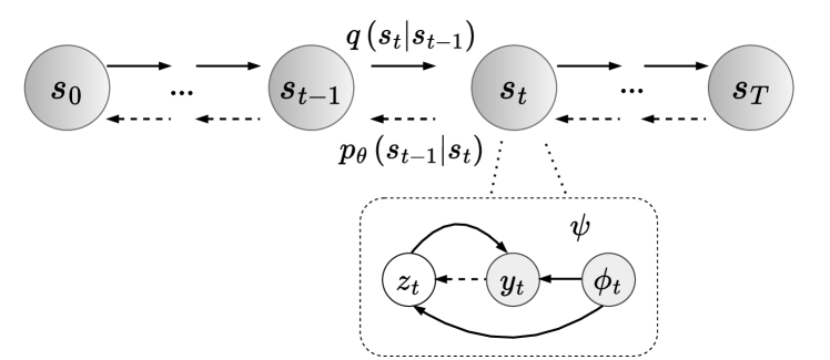
Figure 1: MING Graphical Model. (Top) A forward process $q(s_{t}|s_{t-1})$ defines a noise schedule on function’s output space. We introduce an INR-based denoising network $\theta$ that learns to estimate reverse diffusion processes on function space. (Bottom) A noisy signal $y_{t}$ is a function of trainable latent $z_{t}$ and coordinate-wise inputs $\phi_{t}$. We parameterize the dependency by an another INR-based network $\psi$. The unobserved latent input $z_{t}$ can be obtained from the noisy output $y_{t}$ via gradient-descent optimization.

Representing data as continuous, differentiable functions has become of surging interest for various learning problems [Park et al., 2019, Zhong et al., 2019, Mehta et al., 2021, Dupont et al., 2022]. Intuitively, we represent data as functions that map from some coordinate inputs to signals at the corresponding locations relating to specific data points. A growing area of research explores using neural networks, known as implicit neural representations (INRs), to approximate these functions. These approaches offer some practical advantages for conventional data modalities. First, the network input is element-wise for each coordinate, which allows these networks to represent data at a much higher resolution without intensive memory usage. Second, INRs depend primarily on the choice of coordinate systems, thus a single architecture can be adapted to model various data modalities. Their applications have been explored for the representation tasks of many continuous signals on certain data domains such as images [Sitzmann et al., 2020], 3D shapes [Park et al., 2019], and manifolds [Grattarola and Vandergheynst, 2022].

Recently, an emerging research direction studies generative models over function space. The idea is to learn the distributions of functions that represent data on a continuous space. Several methods, including hyper-networks [Dupont et al., 2021, Du et al., 2021, Koyuncu et al., 2023], latent modulations [Dupont et al., 2022], diffusion probabilistic fields [Zhuang et al., 2023], have addressed some challenging issues when learning functional generative models on regular domains such as images, and spheres. On the other hand, functional generative problems on irregular domains like graphs and manifolds still receive less attention. In a few works, [Elhag et al., 2024, Wang et al., 2024] showed these tasks are feasible. They represent a data function on manifolds by concatenating its signal with coordinate inputs derived from the eigenvectors of graph Laplacians. The graph structure underlying these Laplacians is sampled from the manifold itself. They then apply the standard denoising diffusion probabilistic models [Ho et al., 2020] to learn function distributions, and leverage a modality-agnostic transformer [Jaegle et al., 2021] as denoiser. While these approaches present some promising results, their training regimes rely on this particular architecture, which is computationally expensive and memory-inefficient for the continuous representation objectives.

To the best of our knowledge, we propose the first generative model that learns molecule distributions and generates both bond- and atom- types by exploring their representations in function space. We achieve this by first introducing a new approach to parameterize both molecular-edge- and node- coordinate systems via graph-spectral embeddings. We then propose Molecular Implicit Neural Generation (MING), a novel generative model that applies denoising diffusion probabilistic models on the function space of molecules. Our method presents a new functional denoising objective, which we derive by utilizing an expectation-maximization process to latent implicit neural representations, we thus dub it as the expectation-maximization denoising process. By operating on function space, we are able to simplify the model design, and introduce an INR-based architecture as denoiser. Our model not only benefits from the advantages of INRs but also overcomes the constraints imposed by graph-permutation symmetry, resulting in a model complexity that is less dependent on molecular size. MING effectively captures molecule distributions by generating novel molecules with chemical and structural properties that are closer to test distributions than those generated by other generative models applied to data space. Additionally, MING significantly reduces the number of diffusion/sampling steps required.

2 REPRESENTING MOLECULES AS FUNCTIONS

In this section, we present our approach to parameterize molecules in function space. We first introduce a standard method to represent data as functions by implicit neural representations (INRs). We then showcase how to enable an efficient network parameter sharing between molecules, and eventually to represent data functions on irregular domains such as molecular graph structures.

2.1 Molecule Functions via Conditional INRs

Given a graph denoted by $\mathcal{G}\triangleq\left(X,W\right)$, $X$ and $W$ correspond to the node and edge feature matrices, respectively. We assume for each graph $\mathcal{G}$ there exists a topological space $\mathcal{T}$, and signals $\mathcal{Y}$ living on the topology. For molecular graphs, these signals will be the atom- and bond- types of molecules. We can, thus, represent the structure $\mathcal{G}$ as a mapping or function that maps from the topological space $\mathcal{T}\subset\mathbb{R}^{d}$ to its own signal space $\mathcal{Y}\subset\mathbb{R}^{f}$. A common approach to parameterizing such functions is to use implicit neural representations (INRs) by a neural network ${\theta}:\mathcal{T}\mapsto\mathcal{Y}$.

However, this approach is often costly when one needs to optimize a different set of parameters $\theta^{i}$ for each molecule $\mathcal{G}^{i}\triangleq\left(\mathcal{T}^{i},\mathcal{Y}^{i}\right)$. To enable an efficient parameter sharing between molecules, we leverage the conditional INR networks [Mehta et al., 2021] that introduce a trainable latent-input vector specific to each data point. These INRs define a novel function input space, which is the product of two subspaces $\mathcal{T}\times\mathcal{Z}$ with $\mathcal{Z}\subset\mathbb{R}^{k}$ is a latent unknown manifold. In this way, we can use the shared network $\theta$ and only need to optimize a different latent input for each specific molecule function.

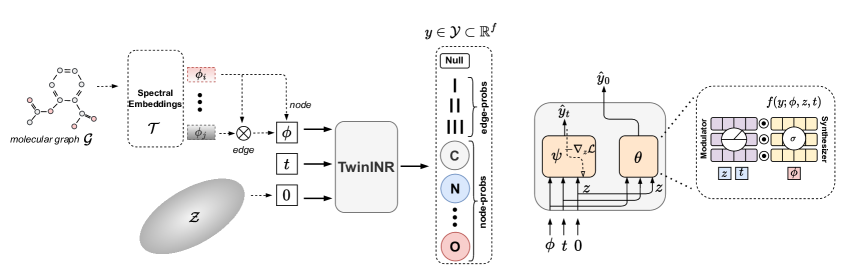
Figure 2: TwinINR Operational Flows. (Left) TwinINR predicts a multi-dimension vector that encodes atom-type, bond-type, and a null token probabilities. While the node-coordinate system $\mathcal{T}$ bases on the eigenvector space of molecular graph Laplacian, we introduce the edge-coordinate system by taking the product of node-coordinate spaces $\mathcal{T}\times\mathcal{T}$. (Right) The TwinINR’s internal architecture composes of two identical (twin) conditional INR networks $\psi$ and $\theta$. The latent network $\psi$ estimates the latent-input representation $z$ of the diffused signal $y_{t}$ at the diffusion step $t$ by maximizing the latent model likelihood. The denoising network $\theta$ predicts the clean signal $y_{0}$ from the noisy latent input $z$. We adapt the latent-modulation strategy [Mehta et al., 2021] for each network.

2.2 Parameterization on Irregular Domains

INRs typically require a coordinate system to define the mapping between domain and signal spaces. These coordinate systems can be easily chosen for data on regular domains such images or spheres. However, it is not clear how to define such coordinate systems for data existing on irregular non-Euclidean ones such as graph structures. In a relevant work [Grattarola and Vandergheynst, 2022] proposed using graph spectral embeddings as the coordinate systems of INRs, where they compute eigenvectors of graph Laplacians and use them as node coordinate inputs. In this work, we further extend this approach to work on edge coordinate systems that will enable functional generative methods to model molecular edge types as well.

For a given graph $\mathcal{G}$, we denote its weighted graph Laplacian by $L_{w}=D-W$, where $D=\text{diag}\left(\text{sum}(W_{c:})\right)$ with $c$ is a column index. Its topological space $\mathcal{T}$ becomes the space of $L_{w}$’s eigenvectors, which we use as node coordinate inputs to INRs, $\phi_{n}\in\mathcal{T}$. In addition, we denote a molecule signal $y\in\mathcal{Y}$, a trainable latent vector $z\in\mathcal{Z}$, and an INR network $\theta$. While modeling node-related information, we have an implicit neural representation, $y={\theta}\left(z,\phi_{n}\right)$ and $y$ encodes atom types, modeling edge information between two nodes $\{i,j\}$, we replace the node coordinate by an edge coordinate as $y={\theta}\left(z,\phi_{n_{i}}\odot\phi_{n_{j}}\right)$ where $y$ encodes edge types and $\odot$ is the Hadamard product. We thus define an edge-coordinate input by directly taking the element-wise product between corresponding node-coordinate inputs, $\phi_{e}\triangleq\phi_{n_{i}}\odot\phi_{n_{j}}$ and $\phi_{n_{i}},\phi_{n_{j}}\in\mathcal{T}$. As the explicit representation of functions is not accessible, we instead represent each function evaluation using a triplet that includes the function’s input and output. Specially, for given a topology input $\phi$, we evaluate its corresponding function output $y$, and define the function evaluation as $s\triangleq(\phi,z,y)$. Here, $\phi$ can be either a node- or edge-coordinate input, $y$ is the associated molecular signal type, and $z$ is a latent input facilitating the parametric representation of functions. We now present functional denoising probabilistic models for molecules.

3 MOLECULAR IMPLICIT NEURAL GENERATION

In this section, we introduce diffusion posteriors within the functional context. Building on this, we propose an expectation-maximization denoising process serving as a core optimization algorithm for functional denoising probabilistic models. We then present a novel INR-based architecture, TwinINR, tailored for denoising tasks. Our generative model focuses on molecule generation problems, to which we refer as molecular implicit neural generation (MING).

3.1 Functional Probabilistic Posteriors

The goal is to train a probabilistic denoising model that maximizes the model likelihood $p_{\theta}\left(s_{0}\right)=\int p_{\theta}\left(s_{0:T}\right)ds_{1:T}$ under the reverse diffusion process $p_{\theta}\left(s_{0:T}\right)$. Following the relevant works [Sohl-Dickstein et al., 2015, Ho et al., 2020], we show that this objective is equivalent to minimizing the Kullback-Leibler divergence between the conditional forward posterior $q(s_{t-1}|s_{t},s_{0})$ and the denoising model posterior $p_{\theta}(s_{t-1}|s_{t})$, where $s_{t}\triangleq(\phi_{t},z_{t},y_{t})$ represents a function evaluation on noisy molecule $\mathcal{G}_{t}$.

A key challenge working on function space is to define noise schedule on forward diffusion process, and learn reverse diffusion process within the space. For the former, since a function maps domain inputs to signal outputs, in this study, we simplify the problem by only diffusing noises on the output space to get noisy functions. Concretely, given a molecular graph $\mathcal{G}_{0}$, which function evaluation on a topology $\phi_{0}$ is $s_{0}\triangleq\left(\phi_{0},z_{0},y_{0}\right)$, we make the following mild assumption:

Assumption 3.1.

The topological information $\phi_{0}$ remains subtly variant throughout the diffusion process, however, the clean signal output, $y_{0}$, which resides on the topological location, undergoes diffusion and converges to a normal prior. This process generates a series of noisy molecular function evaluations $s_{t}\triangleq\left(\phi_{0},z_{t},y_{t}\right)$, where $z_{t}$ is the noisy latent input evolving in response to the diffused signal $y_{t}$.

3.1.1 Conditional Forward Posterior

In the forward process, we apply noise exclusively to the signal component while keeping the topology-input part unchanged. As a result, the posterior satisfies $\phi_{t}\simeq\phi_{0}$ throughout the diffusion process. By expressing the function evaluation in terms of the triplet-based representation, the posterior becomes:

$$q(s_{t-1}|s_{t},s_{0}) =q(\phi_{t-1},z_{t-1},y_{t-1}|\phi_{t},z_{t},y_{t},\phi_{0},z_{0},y_{0})$$

$$=q(z_{t-1},y_{t-1}|z_{t},y_{t},\phi_{0},z_{0},y_{0})$$

$$=q(z_{t-1}|y_{t-1},\phi_{0})q(y_{t-1}|y_{t},y_{0})$$ (1)

The detailed derivation is in Appendix A.1. In the third equality, we apply Bayes’ rule. For the first term, we assume temporal conditional independence between the current latent input $z_{t-1}$ and the function-input $z_{t}$ and output variables $y_{t}$ at other diffusion steps. We formalize this temporal conditional independence by another mild assumption below:

Assumption 3.2.

The latent input variable $z_{t}$ can be reconstructed from its corresponding noisy signal output $y_{t}$ at the same diffusion step and along with the fixed topology input $\phi_{0}$, which is independent to function’s input and output variables evaluated at other diffusion steps.

For the second term, we employ the standard denoising diffusion probabilistic process [Ho et al., 2020] over the signal space $\mathcal{Y}$, which defines its noise kernel and conditional forward posterior as follows:

$$q(y_{t}|y_{0}) =\mathcal{N}(\mu_{y_{t}|y_{0}},\sigma_{y_{t}|y_{0}}^{2}\mathbf{I})$$

$$\mu_{y_{t}|y_{0}}=c_{0}(t)y_{0}$$

$$\sigma_{y_{t}|y_{0}}=c_{1}(t)$$

$$q(y_{t-1}|y_{t},y_{0}) =\mathcal{N}(\mu_{y_{t-1}|y_{t},y_{0}},\sigma_{y_{t-1}|y_{t},y_{0}}^{2}\mathbf{I})$$

$$\mu_{y_{t-1}|y_{t},y_{0}}=c_{2}(t)y_{0}+c_{3}(t)y_{t}$$

$$\sigma_{y_{t-1}|y_{t},y_{0}}=c_{4}(t)$$ (2)

where $c_{i}(t)$s are the diffusion coefficients depending on the diffusion step $t$, as introduced in [Ho et al., 2020].

3.1.2 Denoising Model Posterior

We substitute the triplet-based representation of function evaluation into the denoising model posterior:

$$p_{\theta}(s_{t-1}|s_{t}) =p_{\theta}(z_{t-1},\phi_{t-1},y_{t-1}|z_{t},\phi_{t},y_{t})$$

$$=p_{\theta}(z_{t-1},y_{t-1}|z_{t},\phi_{0},y_{t})$$

$$=p_{\theta}(z_{t-1}|\phi_{0},y_{t-1})p_{\theta}(y_{t-1}|z_{t},\phi_{0},y_{t})$$ (3)

where we apply the topology-input invariance assumption throughout diffusion process to the first equality and the latent temporal conditional independence assumption to the second equality. We visualize the MING’s graphical model in Figure 1.

3.2 Functional Denoising Process

The objective is to minimize the Kullback-Leibler divergence between the functional posteriors at every diffusion step, $\mathcal{L}_{t-1}=D_{KL}(q(s_{t-1}|s_{t},s_{0})\|p_{\theta}(s_{t-1}|s_{t}))$. We prove that the divergence can be simplified into two KL terms optimized directly on the signal and latent spaces by the following proposition:

Proposition 3.1.

For a triplet-based representation of molecule function evaluation $s_{t}\triangleq(\phi_{t},z_{t},y_{t})$, by assuming the topological invariance $\phi_{t}\simeq\phi_{0}$ and the temporal conditional independence of latent posterior $q(z_{t}|\phi_{0},y_{t})$, the KL divergence between two functional posteriors $D_{KL}(q(s_{t-1}|s_{t},s_{0})\|p_{\theta}(s_{t-1}|s_{t}))$ splits into the sum of two KL divergences on the spaces $\mathcal{Z}$ and $\mathcal{Y}$:

$$\mathcal{L}_{t-1} =\mathcal{L}_{t-1}^{\mathcal{Z}}+\mathcal{L}_{t-1}^{\mathcal{Y}}$$

$$=\mathbb{E}_{q(y_{t-1}|y_{t},y_{0})} \left(D_{KL}\left(q(z_{t-1}|y_{t-1},\phi_{0})\|p_{\theta}(z_{t-1}|y_{t-1},\phi_{0})\right)\right)$$

$$+D_{KL}\left(q(y_{t-1}|y_{t},y_{0})\|p_{\theta}(y_{t-1}|z_{t},\phi_{0},y_{t})\right)$$ (4)

We give the proof in Appendix A.3. The first term, $\mathcal{L}_{t-1}^{\mathcal{Z}}$, represents the KL divergence computed over the latent-input space $\mathcal{Z}$, which then takes the expectation w.r.t the conditional forward posterior on the signal space $\mathcal{Y}$. The second term, $\mathcal{L}_{t-1}^{\mathcal{Y}}$, quantifies the KL divergence between two posteriors on $\mathcal{Y}$. Below, we will analyse the KL minimization problem on each space.

3.2.1 Gradient Origin $z$-based Optimization

We now analyse the KL term $\mathcal{L}_{t-1}^{\mathcal{Z}}$ on the latent-input space $\mathcal{Z}$. However, there are no closed-form solutions for the posteriors of latent variable $z_{t-1}$. We thus approach this task as a likelihood-maximization problem given a noisy observed signal $y_{t-1}$, an observed topology $\phi_{0}$, and an unobserved latent input $z_{t-1}$. To achieve this, we introduce a latent model $p_{\psi}(z_{t-1},y_{t-1},\phi_{0})$ parameterized by an auxiliary INR network $\psi$ that learns the mapping between noisy function’s output and inputs, ${\psi}:\phi_{0}\times z_{t-1}\mapsto y_{t-1}$. We can show that the KL term $\mathcal{L}_{t-1}^{\mathcal{Z}}$ converges to zeros by the next proposition:

Proposition 3.2.

For the likelihood optimization problem involving the latent model $p_{\psi}(z_{t-1},y_{t-1},\phi_{0})$ shared across both the denoising-model, $p_{\theta}(z_{t-1}|y_{t-1},\phi_{0})$, and conditional forward, $q(z_{t-1}|y_{t-1},\phi_{0})$, posteriors on $\mathcal{Z}$, the KL divergence $\mathcal{L}_{t-1}^{\mathcal{Z}}$ between the two posteriors converges to zeros as they have the same empirical distribution at each reverse diffusion step, or $\mathcal{L}_{t-1}^{\mathcal{Z}}\rightarrow 0$.

Proof: We remark that these two latent posteriors are conditioned on the same factors, namely $\phi_{0}$ and $y_{t-1}\sim q(y_{t-1}|y_{0},y_{t})$. By employing the same latent model $p_{\psi}(z_{t-1},y_{t-1},\phi_{0})$ applied to both the denoising-model and conditional forward posteriors, we observe that these posteriors exhibit similar latent distributions in $\mathcal{Z}$. A more detailed proof is in Appendix A.4.

However, we still need to estimate the noisy-latent input $z_{t}$ for the denoising process. Inspired by similar work [Bond-Taylor and Willcocks, 2021], we first initialize the latent-input variable $z_{t}$ at the origin of an unknown manifold $\mathcal{Z}$ and iteratively optimize $z_{t}$ and $\psi$ by gradient descent to maximize the latent model log likelihood $p_{\psi}(z_{t},y_{t},\phi_{0})$, which is equivalent to minimize the reconstruction loss in the signal space $\mathcal{Y}$:

$$\mathcal{L}_{out}(\psi)=\int\mathcal{L}\left(y_{t},{\psi}\left(\phi_{0},\underbrace{-\nabla_{z_{t}}\int\mathcal{L}\left(y_{t},{\psi}(\phi_{0},z_{t})\right)d\phi_{0}}_{\mathcal{L}_{in}(z_{t})}\right)\right)d\phi_{0}$$ (5)

where $\mathcal{L}$ denotes the mean-squared error loss, and both integrals are evaluated over the topological space $\mathcal{T}$. The main objective consists of two loss components. The first term, referred as the inner loss $\mathcal{L}_{in}(z_{t})$, involves fixing the network parameters $\psi$ while optimizing $z_{t}$, which is initially set at the origin. The second term, known as the outer loss $\mathcal{L}_{out}(\psi)$, involves optimizing the network parameters $\psi$ using the $z_{t}$ derived from the inner-optimization step. These two steps are analogous to performing the expectation-maximization (EM) optimization over the latent model $p_{\psi}(z_{t},y_{t},\phi_{0})$. Below, we introduce a novel training objective for diffusion models applied in function space.

3.2.2 E-M Denoising Objective

Algorithm 1 Molecular Implicit Neural Generation.

  Input: denoiser $\theta$, latent model $\psi$, $T$ diffusion steps, training set $\mathcal{D}_{train}$. /* Training */

  for $(\phi_{0}=\phi_{n}[,\phi_{e}],y_{0})\in\mathcal{T}^{i}\left[\times\mathcal{T}^{i}\right]\times\mathcal{Y}^{i}\sim\mathcal{D}_{train}$:

      $t\sim\mathcal{U}_{[0,T]}$

      $y_{t}\sim\mathcal{N}\left(\mu_{y_{t}|y_{0}},\sigma_{y_{t}|y_{0}}^{2}\mathbf{I}\right)$

      $z_{t}\leftarrow 0$

      for # iterations:

         $\hat{y}_{t}\leftarrow{\psi}\left(z_{t},\phi_{0}\right)$

         $\mathcal{L}_{e}\leftarrow\|\hat{y}_{t}-y_{t}\|^{2}$

         $z_{t}\leftarrow\text{gradient\_descent}\left(\nabla_{z_{t}}\mathcal{L}_{e}\right)$ {E-step}

      $\hat{y}_{0},\hat{y}_{t}\leftarrow{\theta}\left(z_{t},\phi_{0}\right),{\psi}\left(z_{t},\phi_{0}\right)$

      $\mathcal{L}_{m}\leftarrow\|\hat{y}_{t}-y_{t}\|^{2}+\|\hat{y}_{0}-y_{0}\|^{2}$

      $\theta,\psi\leftarrow\text{adam}\left(\nabla_{\theta,\psi}\mathcal{L}_{m}\right)$ {M-step} /* Sampling */

  $y_{T}\sim\mathcal{N}\left(0,I\right)$

  $\phi_{0}=\phi_{n}[,\phi_{e}]\in\mathcal{T}^{i}\left[\times\mathcal{T}^{i}\right]\sim\mathcal{D}_{train}$

  for t $\rightarrow$ $[T,0)$:

      $z_{t}\leftarrow 0$

      for # iterations:

         $\hat{y}_{t}\leftarrow{\psi}\left(z_{t},\phi_{0}\right)$

         $z_{t}\leftarrow\text{gradient\_descent}\left(\nabla_{z_{t}}\|\hat{y}_{t}-y_{t}\|^{2}\right)$

      $y_{t-1}\leftarrow\mathcal{N}(\mu_{y_{t-1}|z_{t},\phi_{0},y_{t}},\sigma_{y_{t-1}|z_{t},\phi_{0},y_{t}}^{2}\mathbf{I})$

  return: $y_{0}$

By substituting the previous result, $\mathcal{L}_{t-1}^{\mathcal{Z}}\rightarrow 0$, into the KL divergence in Equation 3.2, we now only need to minimize the KL divergence term on $\mathcal{Y}$: $\displaystyle\mathcal{L}_{t-1}=\mathcal{L}_{t-1}^{\mathcal{Y}}=D_{KL}\left(q(y_{t-1}|y_{t},y_{0})\|p_{\theta}(y_{t-1}|z_{t},\phi_{0},y_{t})\right)$ (6) The conditional forward posterior $q(y_{t-1}|y_{t},y_{0})$ is given in Equation 3.1.1, which we utilize to parameterize the denoising model posterior on the signal space:

$$p_{\theta}(y_{t-1} |z_{t},\phi_{0},y_{t})=\mathcal{N}(\mu_{y_{t-1}|z_{t},\phi_{0},y_{t}},\sigma_{y_{t-1}|z_{t},\phi_{0},y_{t}}^{2})$$

$$\mu_{y_{t-1}|z_{t},\phi_{0},y_{t}}=c_{2}(t)\hat{y}_{0}+c_{3}(t)y_{t}$$

$$\qquad\qquad\quad\,\,=c_{2}(t){\theta}(\phi_{0},z_{t})+c_{3}(t)y_{t}$$

$$\sigma_{y_{t-1}|z_{t},\phi_{0},y_{t}}=c_{4}(t)$$ (7)

Here, the INR denoiser $\theta$ predicts the clean signal $y_{0}$ from the noisy latent input $z_{t}$ and the coordinate input $\phi_{0}$. Similar to the approach in [Ho et al., 2020], we can derive the denoising objective on $\mathcal{Y}$ as $\mathcal{L}_{t-1}=\|{\theta}(\phi_{0},z_{t})-y_{0}\|^{2}$, with $z_{t}$ optimized from the E-M process on the latent model $p_{\psi}(z_{t},y_{t},\phi_{0})$ in Equation 5. We thus refer the overall optimization as the expectation maximization denoising process. At every diffusion step, we solve two sub-optimization problems:

Expectation Step

We optimize the noisy latent input value $z_{t}$, initially set to the origin, by minimizing the inner loss $\mathcal{L}_{in}(z_{t})$ with gradient descent, the expectation loss $\mathcal{L}_{e}$ is equal to the inner loss $\mathcal{L}_{e}=\mathcal{L}_{in}(z_{t})$.

Maximization Step

We jointly optimize the parameters of denoiser $\theta$ using the denoising objective loss $\mathcal{L}_{t-1}$, while simultaneously optimizing the latent model parameters $\psi$ to maximize the latent model likelihood, given the obtained representation $z_{t}$, through $\mathcal{L}_{out}(\psi)$; we get the maximization loss as $\mathcal{L}_{m}=\mathcal{L}_{t-1}+\mathcal{L}_{out}(\psi)$.

3.3 Training and Sampling

In training, we use the node coordinates $\phi_{0}=\phi_{n}$, edge coordinates $\phi_{0}=\phi_{e}$, and their corresponding signals $y_{0}$ of molecular graphs $\mathcal{G}^{i}\triangleq\left(\mathcal{T}^{i},\mathcal{Y}^{i}\right)$, which we sample from a training set $\mathcal{D}_{train}$. At each diffusion step, with $t$ uniformly distributed, $\mathcal{U}_{[0,T]}$, we initialize the latent input variable $z_{t}$ with a zero-valued vector and optimize the expectation maximisation denoising objective.

To generate novel molecules, we first sample node and edge coordinate inputs from the training set $\phi_{0}=\phi_{n}[,\phi_{e}]\in\mathcal{T}^{i}\left[\times\mathcal{T}^{i}\right]\sim\mathcal{D}_{train}$, and then initialize their signals from the normal prior $y_{T}\sim\mathcal{N}\left(0,I\right)$. We apply the reverse functional diffusion process, in which we only optimize the expectation objective at each reverse step to get the final generated signals, $y_{t=0}$. We summarize MING in Algorithm 1.

3.4 TwinINR as Denoiser Architecture

We design the denoising architecture using implicit-neural-representations (INRs), which consist of a stack of MLP layers combined with nonlinear activation functions. The architecture includes two identical INRs, namely TwinINR. The first module is the latent model network $\mathcal{\psi}$ that represents the noisy molecule function evaluations $s_{t}\triangleq(\phi_{0},z_{t},y_{t})$. The second module often refers as the denoising network $\theta$ that predicts the clean signal $y_{0}$ from the perturbed latent input $z_{t}$ and the coordinate input $\phi_{0}$. We adopt the modulated conditional INR architecture [Mehta et al., 2021] that allows for the efficient parameter sharing between molecule samples. Moreover, we extend the existing architecture to work on arbitrary domains, moving beyond regular vertex spaces like image or sphere domains, by using coordinates computed from graph spectral embeddings.

The two components $\psi$ and $\theta$ share the same architecture design, with each containing a synthesis network and a modulation one. The synthesis network generates the signal output $y$ from the corresponding coordinate $\phi_{0}$, each layer is an MLP equipped with a nonlinear activation function:

$$h_{i}=\alpha_{i}\odot\sigma(w_{i}h_{i-1}+b_{i})$$ (8)

where $h_{i}$ is the hidden feature at the $i$-th layer and $h_{0}=\phi_{0}$, $w_{i}$ and $b_{i}$ are the learnable weights and biases for the $i$-th MLP layer, $\sigma$ is a nonlinear activation, and $\alpha_{i}$ is the modulation vector that modulates the hidden feature output using the pointwise multiplication. We model the hidden modulation features using the modulation network, which is an another MLP stack with the activation ReLU:

$$\alpha_{0} =\text{ReLU}\left(w_{0}^{{}^{\prime}}z+b_{0}^{{}^{\prime}}\right)$$

$$\alpha_{i} =\text{ReLU}\left(w_{i}^{{}^{\prime}}[\alpha_{i-1}\;z]^{T}+b_{i}^{{}^{\prime}}\right)$$ (9)

where $w_{i}^{{}^{\prime}}$ and $b_{i}^{{}^{\prime}}$ represent the weights and biases. Note that the latent input $z$ is concatenated at each layer of the modulation network. We illustrate TwinINR in Figure 2.

4 EXPERIMENTS

Table 1: Comparisons with the models trained on the graph representation of molecules. The baseline results are sourced from GDSS [Jo et al., 2022]. The detailed results with standard deviations are in Appendix B.2.

Method		QM9			ZINC250k
		Val. $(\%)\uparrow$	NSPDK $\downarrow$	FCD $\downarrow$	Val. $(\%)\uparrow$	NSPDK $\downarrow$	FCD $\downarrow$
Graph	GraphAF [Shi et al., 2020]	74.43	0.021	5.63	68.47	0.044	16.02
	GraphDF [Luo et al., 2021]	93.88	0.064	10.93	90.61	0.177	33.55
	GDSS [Jo et al., 2022]	95.72	0.003	2.90	97.01	0.019	14.66
	GraphArm [Kong et al., 2023]	90.25	0.002	1.22	88.23	0.055	16.26
Function	MING	98.23	0.002	1.17	97.19	0.005	4.80

Table 2: Comparisons with the models trained on the sequence-based representation of molecules on QM9. The baseline results are taken from [De Cao and Kipf, 2018].

Method		Val.$\uparrow$	Uni.$\uparrow$	Nov.$\uparrow$
Sequence	Character-VAE	10.3	67.5	90.0
	Grammar-VAE	60.2	9.3	80.9
Function	MING	98.23	96.83	71.59

4.1 Experimental setup

Datasets

We validate MING on the ability to learning complex molecule structures in function space. We benchmark on two standard molecule datasets. QM9 [Ramakrishnan et al., 2014] contains an enumeration of small chemical valid molecules of 9 atoms, which compose of 4 atom types fluorine, nitrogen, oxygen, and carbon. ZINC250k [Irwin et al., 2012] is a larger molecule dataset that contains molecules up to the size of 38 atoms. In addition, the dataset composes of 9 different atom types, which exposes more diverse structural and chemical molecular properties. Following [Jo et al., 2022], we kekulize molecules by RDKit [Landrum et al., 2016] and remove hydrogen atoms.

Metrics

We measure molecule-generation statistics in terms of validity without correction (Val.), which is the percentage of chemical-valid molecules without valency post-hoc correction. Among the valid generated molecules, we compute uniqueness (Uni.) and novelty (Nov.) scores, which measure the percentage of uniquely generated and novel molecules compared to training sets, respectively. Besides the generation statistics, we quantify how well generated molecule distributions align with test distributions by computing two more salient metrics, namely Fréchet ChemNet Distance (FCD) [Preuer et al., 2018] and Neighborhood Subgraph Pairwise Distance Kernel (NSPDK) [Costa and Grave, 2010]. While FCD computes the chemical distance between two relevant distributions, NSPDK measures their underlying graph structure similarity. These two metrics highlight more precisely the quality of generated molecules by taking into account molecule’s structural and chemical properties rather than only their generation statistics.

Implementations

We adhere to the evaluation protocol outlined in GDSS [Jo et al., 2022], in which we utilize the same data splits. To assess the impact of hyperparameter settings, we ablate different hidden feature dimensions $\{64,128,256\}$, latent-z dimensions $k\in\{8,16\}$, coordinate-input dimensions $d\in\{10,20,30,37\}$ on ZINC250k and $d\in\{5,7,9\}$ on QM9. We set the inner optimization iterations to three for all experiments. We observe that MING performs competitively with only 100 diffusion steps on QM9 and 30 diffusion steps on ZINC250k. The main reported results represent the mean of three samplings, each consisting of 10000 sampled molecules. Detailed hyperparameter settings can be found in Appendix B.2.

4.2 Baselines

We benchmark MING against two types of molecular generative models, which utilize either the sequence-based or graph-based representation of molecules. Specifically, we compare with Grammar-VAE [Kusner et al., 2017], Character-VAE [Gómez-Bombarelli et al., 2018], they apply variational autoencoders to SMILES-based representations. On the graph space, we compare with GraphAF [Shi et al., 2020], an continuous auto-regressive flow model, GraphDF [Luo et al., 2021], a flow model for the discrete setting, GDSS [Jo et al., 2022], an continuous graph score-based framework, and GraphArm [Kong et al., 2023], an auto-regressive diffusion model.

4.3 Results

Graph Generation Statistics

We evaluate the graph generation statistics based on validity, uniqueness, and novelty. Table 1 suggests that MING demonstrates competitive performance in sampling novel, chemical valid molecules compared with the graph-based baselines. We attribute this result as MING removes the graph-permutation constraint by generating signals directly on the topology inputs of data, a process typically employed in function-based generative frameworks. In contrast, the baselines struggle to learn the graph symmetry by either pre-assuming a canonical ordering on molecular graphs or using complex equivariant architectures. Compared with the sequence-based models, Table 2 shows that MING significantly outperforms both Character- and Grammar-VAE on QM9. These string-based models hardly learn valency rules between atom and bond types to compose valid, unique molecules. For QM9, models with high validity scores often generate lower novel molecules. This is due to the fact that the dataset enumerates all possible small valid molecules composed of only four atoms. However, this problem can be alleviated when training on larger molecule datasets like ZINC250k, where we observe that MING consistently achieves near-perfect novelty scores when its validity exceeds 99$\%$.

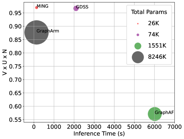
Figure 3: Model efficiency benchmarking on ZINC250k.

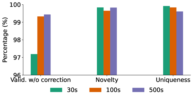
Figure 4: V.U.N performance within different number of diffusion steps $T$ on ZINC250k.

Distribution-based Distance Metrics

Table 1 shows that MING generates novel molecules that closely match to the test distributions in terms of chemical and biological properties, measured by the FCD metric, outperforming other generative models. On the large scale dataset ZINC250k, MING demonstrates its advantages clearly when improving the FCD metric $3\times$ compared to the best baseline, GDSS. This highlights a promising result of learning chemical molecular properties in function space. On learning molecular graph structures, MING also generates underlying molecule substructures including bond- and atom- types closer to the test distributions, as measured by the NSPDK metric. This function-based modeling advantage can be clearly observed when training on large-scale molecules.

Speed, Memory and Model Performance

We benchmark the model efficiency by generating 10000 molecules on a Titan RTX of 8 CPU cores. Figure 3 visualizes the necessary inference time, number of model parameters, and performance, measured by the product of validity, uniqueness, and novelty VxUxN. We observe that MING proves a remarkable efficiency, using $317\times$ fewer parameters than the fastest baseline, GraphArm, while maintaining superior performance. MING is also faster than the best-performing baseline, GDSS, which applies continuous score-based models on the graph representation of molecules. Compared to the auto-regressive flow baseline GraphAF, MING significantly improves across all criteria. We do not report the model efficiency of GraphDF as this framework has a similar model size to GraphAF, but $10\times$ slower in inference speed.

Ablation on Diffusion Steps

We asses the MING’s generation capability by ablating different number of diffusion steps, $T\in\{30,100,500\}$, on ZINC250k. We train models with the same set of hyper-parameters except for the diffusion steps $T$. Figure 4 presents the mean validity, uniqueness, novelty (V.U.N) results on three samplings of 10000 molecules. We observe that, utilizing higher diffusion steps, $T\in\{100,500\}$, MING can achieve over 99$\%$ validity scores. Furthermore, all experimented models consistently surpass 99.5$\%$ for both uniqueness and novelty scores. By working on the function space of molecules, MING significantly speed up the sampling process for diffusion models without causing a dramatic performance drop.

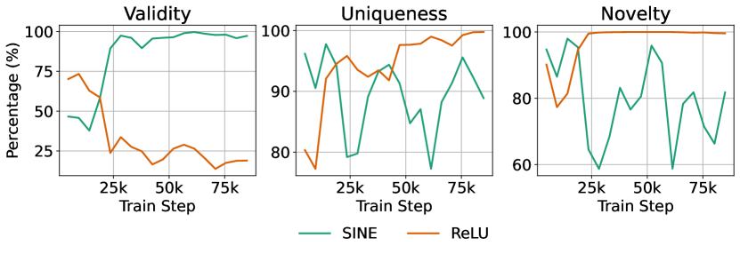
Figure 5: V.U.N performance with SINE and ReLU activation functions on QM9.

Ablation on non-Linear Activation Functions

We study the impact of synthesizer’s activation function, $\sigma$, on model performance. We train two models with the same hyper-parameter set, applying the Sinusoidal activation (SINE) on one model and the activation ReLU on the other. Figure 5 shows the V.U.N results on 10000 sampled molecules during the course of training process. We remark that the synthesizer with ReLU is incapable of modeling molecular signals on their topological space, leading to low validity scores for the generated molecules. On the other hand, the synthesizer using the activation SINE learns better the function representation of molecules, mapping from topological inputs to molecular signals. These findings are consistent with [Sitzmann et al., 2019], where they first experimented the Sinusoidal activation function for representing complex data signals on regular domains.

5 Conclusion

This paper introduces MING, a generative model that learns molecule distributions in function space by optimizing an expectation-maximization denoising objective. MING is, to our knowledge, the first function-based generative model capable of generating both bond and atom types of molecules. Our experiments on molecule datasets demonstrate several advantages of leveraging functional representations for molecule generation, including faster inference speed, smaller model size, and improved performance in capturing molecule distributions as measured by statistics-based and distribution-based metrics. Unlike graph-based models, MING avoids the complexities of graph-permutation symmetry, streamlining model architecture design. This approach could align with recent research exploring the potential of non-equivariant molecular generative models. In future work, we aim to extend the MING framework to address broader molecule-related problems in function space, such as molecule conformation and full 3D physical structure generation.

Appendix A MING’s DERIVATION DETAILS

We present denoising diffusion probabilistic models applied to the function representation of molecules. In this framework, we represent each molecule function as a set of function evaluations over its input domain, formally defined as:

$$f_{0}\triangleq\{s_{0}\triangleq(\phi_{0},z_{0},y_{0})|\phi_{0}\in\mathcal{T},z\in\mathcal{Z},y\in\mathcal{Y}\}$$ (10)

where $\mathcal{T}$ is the molecule input domain, $\mathcal{Y}$ is the corresponding molecular signals on $\mathcal{T}$, $\mathcal{Z}$ is an unknown latent manifold, and $s_{0}$ is the function evaluation on the topology input $\phi_{0}$. Following the approach from [Sohl-Dickstein et al., 2015, Ho et al., 2020], we want to learn a model $\theta$ that maximizes the likelihood given an initial function evaluation $s_{0}$. This can be formulated as:

$$p_{\theta}(s_{0})=\int p_{\theta}(s_{0:T})ds_{1:T}$$ (11)

where $s_{1:T}$ represents a series of noised function evaluations during the diffusion process. However, directly evaluating the likelihood is intractable, we sort to the relative evaluation between the forward and reverse process, averaged over the forward process [Sohl-Dickstein et al., 2015]:

$$p_{\theta}(s_{0}) =\int p_{\theta}(s_{0:T})ds_{1:T}$$

$$=\int p_{\theta}(s_{0:T})\frac{q(s_{1:T}|s_{0})}{q(s_{1:T}|s_{0})}ds_{1:T}$$

$$=\int p_{\theta}(s_{0:T})\frac{q(s_{1:T}|s_{0})}{q(s_{1:T}|s_{0})}ds_{1:T}$$

$$=\int p_{\theta}(s_{T})q(s_{1:T}|s_{0})\prod\frac{p_{\theta}(s_{t-1}|s_{t})}{q(s_{t}|s_{t-1})}ds_{1:T}$$

where $q(s_{1:T}|s_{0})=\prod q(s_{t}|s_{t-1})$ defines a Markovian forward trajectory. Training involves minimizing the lower bound of the negative log likelihood:

$$\mathbb{E}_{q(s_{1:T}|s_{0})}\left[-\log p_{\theta}(s_{0})\right]\leq\mathbb{E}_{q(s_{1:T}|s_{0})}\left[-\log\frac{p_{\theta}(s_{0:T})}{q(s_{1:T}|s_{0})}\right]\triangleq\mathcal{L}_{\theta}$$ (13)

This can further be decomposed into a sum over diffusion steps:

$$\mathcal{L}_{\theta}=\mathbb{E}_{q(s_{1:T}|s_{0})}\left[\underbrace{-\log p_{\theta}(s_{0}|s_{1})}_{\mathcal{L}_{0}}+\sum_{t=2}^{T}\underbrace{D_{KL}\left(q(s_{t-1}|s_{t},s_{0})\|p_{\theta}(s_{t-1}|s_{t})\right)}_{\mathcal{L}_{t-1}}+\underbrace{D_{KL}\left(q(s_{T}|s_{0})\|p_{\theta}(s_{T})\right)}_{\mathcal{L}_{T}}\right]$$ (14)

where $q(s_{t-1}|s_{t},s_{0})$ and $p_{\theta}(s_{t-1}|s_{t})$ are the forward conditional and denoising model posteriors which we analyse in the functional setting as follows.

A.1 Conditional Forward Posterior

Substituting the triplet-based function evaluation to the conditional forward posterior we have:

$$q(s_{t-1}|s_{t},s_{0}) =q(\phi_{t-1},z_{t-1},y_{t-1}|\phi_{t},z_{t},y_{t},\phi_{0},z_{0},y_{0})$$

$$=q(\phi_{0},z_{t-1},y_{t-1}|\phi_{0},z_{t},y_{t},\phi_{0},z_{0},y_{0})$$ (topology-input invariance.)

$$=q(z_{t-1},y_{t-1}|z_{t},y_{t},\phi_{0},z_{0},y_{0})$$

$$=q(z_{t-1}|z_{t},y_{t},y_{t-1},\phi_{0},z_{0},y_{0})q(y_{t-1}|z_{t},y_{t},\phi_{0},z_{0},y_{0})$$

$$=q(z_{t-1}|y_{t-1},\phi_{0})q(y_{t-1}|z_{t},y_{t},\phi_{0},z_{0},y_{0})$$ (latent temporal conditional independence.)

$$=q(z_{t-1}|y_{t-1},\phi_{0})q(y_{t-1}|\underbrace{\phi_{0},z_{t}}_{y_{t}},y_{t},\underbrace{\phi_{0},z_{0}}_{y_{0}},y_{0})$$

$$=q(z_{t-1}|y_{t-1},\phi_{0})q(y_{t-1}|y_{t},y_{0})$$ (15)

A.2 Denoising Model Posterior

In a similar way we derive the denoising model posterior:

$$p_{\theta}(s_{t-1}|s_{t}) =p_{\theta}(z_{t-1},\phi_{t-1},y_{t-1}|z_{t},\phi_{t},y_{t})$$

$$=p_{\theta}(z_{t-1},\phi_{0},y_{t-1}|z_{t},\phi_{0},y_{t})$$ (topology-input invariance.)

$$=p_{\theta}(z_{t-1},y_{t-1}|z_{t},\phi_{0},y_{t})$$

$$=p_{\theta}(z_{t-1}|z_{t},\phi_{0},y_{t},y_{t-1})p_{\theta}(y_{t-1}|z_{t},\phi_{0},y_{t})$$

$$=p_{\theta}(z_{t-1}|\phi_{0},y_{t-1})p_{\theta}(y_{t-1}|\underbrace{z_{t},\phi_{0}}_{\hat{y}_{0}},y_{t})$$ (latent temporal conditional independence.) (16)

A.3 Proof of Proposition 3.1

In order to prove Proposition 3.1, we replace the functional posterior forms above to the KL term $\mathcal{L}_{t-1}$:

$$\mathcal{L}_{t-1} =D_{KL}(q(s_{t-1}|s_{t},s_{0})\|p_{\theta}(s_{t-1}|s_{t}))$$

$$=\int q(s_{t-1}|s_{t},s_{0})\log\frac{q(s_{t-1}|s_{t},s_{0})}{p_{\theta}(s_{t-1}|s_{t})}ds_{t-1}$$

$$=\int\int q(z_{t-1}|y_{t-1},\phi_{0})q(y_{t-1}|y_{t},y_{0})\log\frac{q(z_{t-1}|y_{t-1},\phi_{0})q(y_{t-1}|y_{t},y_{0})}{p_{\theta}(z_{t-1}|\phi_{0},y_{t-1})p_{\theta}(y_{t-1}|z_{t},\phi_{0},y_{t})}dz_{t-1}dy_{t-1}$$

$$=\int\int q(z_{t-1}|y_{t-1},\phi_{0})q(y_{t-1}|y_{t},y_{0})\log\frac{q(z_{t-1}|y_{t-1},\phi_{0})}{p_{\theta}(z_{t-1}|\phi_{0},y_{t-1})}dz_{t-1}dy_{t-1}$$

$$\qquad\qquad\qquad+\int\int q(z_{t-1}|y_{t-1},\phi_{0})q(y_{t-1}|y_{t},y_{0})\log\frac{q(y_{t-1}|y_{t},y_{0})}{p_{\theta}(y_{t-1}|z_{t},\phi_{0},y_{t})}dz_{t-1}dy_{t-1}$$

$$=\int\int q(z_{t-1}|y_{t-1},\phi_{0})\log\frac{q(z_{t-1}|y_{t-1},\phi_{0})}{p_{\theta}(z_{t-1}|\phi_{0},y_{t-1})}dz_{t-1}\;q(y_{t-1}|y_{t},y_{0})dy_{t-1}$$

$$\qquad\qquad\qquad+\int q(y_{t-1}|y_{t},y_{0})\log\frac{q(y_{t-1}|y_{t},y_{0})}{p_{\theta}(y_{t-1}|z_{t},\phi_{0},y_{t})}dy_{t-1}\underbrace{\int q(z_{t-1}|y_{t-1},\phi_{0})dz_{t-1}}_{constant}$$

$$=\mathbb{E}_{q(y_{t-1}|y_{t},y_{0})}\left(D_{KL}\left(q(z_{t-1}|y_{t-1},\phi_{0})\|p_{\theta}(z_{t-1}|y_{t-1},\phi_{0})\right)\right)+D_{KL}\left(q(y_{t-1}|y_{t},y_{0})\|p_{\theta}(y_{t-1}|z_{t},\phi_{0},y_{t})\right)$$

$$=\mathcal{L}_{t-1}^{\mathcal{Z}}+\mathcal{L}_{t-1}^{\mathcal{Y}}$$ (17)

We have the KL term $\mathcal{L}_{t-1}$ can be directly optimized on the latent input space, $\mathcal{Z}$, and signal output space, $\mathcal{Y}$.

A.4 Proof of Proposition 3.2

Given a latent model $p_{\psi}\left(z,\phi,y\right)=p(z,\phi,y|\psi)$ where $\psi:\phi\times z\rightarrow y$ models the relation between the topology input $\phi$, latent variable $z$, and signal output $y$. For an observed pair of topology input and signal $(\phi,y)$, we look for $z$ to minimize an optimization problem:

$$z=\operatorname*{arg\,min}_{z}\|\psi(\phi,z)-y\|^{2}$$ (18)

Since $\psi$ is an INR network, which is differentiable and deterministic, the loss gradient w.r.t $z$ is thus uniquely determined for each value of $z$. By using gradient descent optimization to the minimization problem, at the step $k+1$ we have $z_{t+1}$ is uniquely defined:

$$z_{k+1}=z_{k}-\nabla_{z_{k}}\|\psi(\phi,z_{k})-y\|^{2}$$ (19)

We apply the latent model $p(z,\phi,y|\psi)$ to the conditional forward posterior $q(z_{t-1}|y_{t-1},\phi_{0})$ and the denoising model posterior $p_{\theta}(z_{t-1}|y_{t-1},\phi_{0})$. Since these posteriors are conditioned on the same topology input and signal output $(\phi_{0},y_{t-1}\sim q(y_{t-1}|y_{t},y_{0}))$, the latent model results in the same latent-input representation $z_{t-1}$ for both posteriors.

Appendix B EXPERIMENTAL DETAILS

B.1 Additional Experiments

B.1.1 Ablation on Topological Input Dimensions

We investigate the impact of structural changes in the topology input, $\phi$, on model denoising efficiency. We experiment on ZINC250k as the dataset features a high topological dimension, with $k_{max}=38$. Figure 6 shows the denoising loss, $\mathcal{L}_{t-1}(\theta)$, and maximization loss, $\mathcal{L}_{m}(\theta,\psi)$, across different topology-input sizes. We observe that MING can achieve more effective denoising with higher-dimensional inputs. However, when experimenting nearly the full topological dimension of the data, $k=37$, the model’s denoising ability slightly declines. Utilizing an suitable dimension allows MING to generalize well across varying molecule’s topological input spaces.

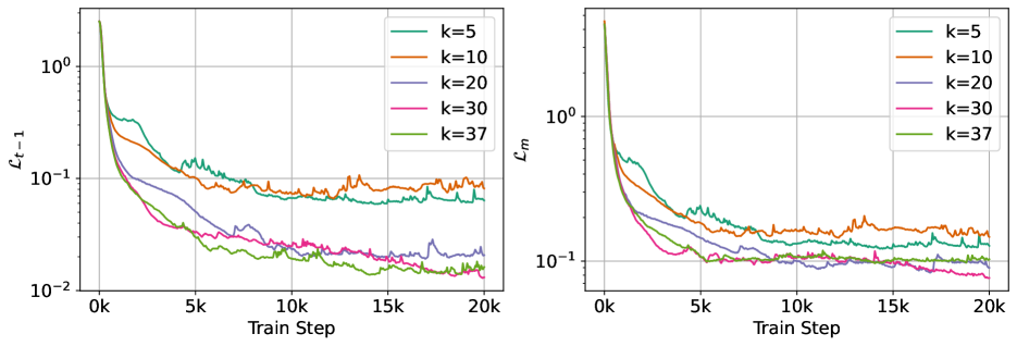
Figure 6: Ablation study on topological input dimensions. The denoising objective loss (left), $\mathcal{L}_{t-1}(\theta)$, and maximization objective loss (right), $\mathcal{L}_{m}(\theta,\psi)$, for different topological input dimensions, $k$.

B.1.2 Ablation on Inner Optimization Steps

We ablate the effect of inner optimization steps on the expectation objective loss, $\mathcal{L}_{e}(z_{t})$. As depicted in Figure 7, MING significantly reduces the expectation loss and stabilizes latent input learning with a higher number of optimisation steps. Moreover, choosing an appropriate iterations is essential for balancing the tradeoff between MING’s inference speed and performance.

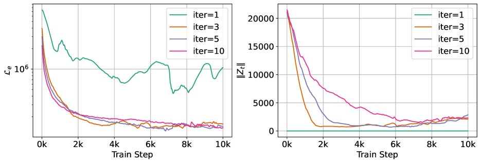
Figure 7: Ablation study on inner optimization steps. The sum of expectation objective losses (left), $\mathcal{L}_{e}(z_{t})$, and z-norm regularisation (right) for different numbers of inner optimisation steps.

B.2 Main Experiments

B.2.1 Hyperparameters

Table 3: MING hyperparameters.

	Hyperparam	QM9	ZINC250k
$\phi,\psi$	topology-input dimension $d$	7	30
	hidden dimension	256	64
	latent dimension $k$	64	8
	signal dimension $f$	8	13
	number layers	8	3
SDE	$\beta_{\min}$	0.0001	0.0001
	$\beta_{\max}$	0.02	0.02
	diffusion steps $T$	100	30
MING	$\mathcal{L}_{e}$ optimizer	Gradient descent	Gradient descent
	$\mathcal{L}_{m}$ optimizer	Adam	Adam
	$\mathcal{L}_{e}$ learning rate	0.1	0.1
	$\mathcal{L}_{m}$ learning rate	0.0001	0.001
	$\mathcal{L}_{e}$ number optimisation steps	3	3
	batch size	256	256
	number of epochs	500	500

B.2.2 Detailed Results

Table 4: Statistics of molecule graphs on QM9 and ZINC250k.

	Graphs	Nodes	Node Types	Edge Types
QM9	$133885$	$1\leqslant|X|\leqslant 9$	$4$	$3$
ZINC250k	$249455$	$6\leqslant|X|\leqslant 38$	$9$	$3$

Table 5: MING’s main results, including the mean and standard deviations for three sampling times, each with 10000 sampled molecules.

	Val. $\uparrow$	Uni. $\uparrow$	Nov. $\uparrow$	NSPDK $\downarrow$	FCD $\downarrow$
ZINC250k	97.19 $\pm$ 0.09	99.92 $\pm$ 0.03	99.84 $\pm$ 0.06	0.005 $\pm$ 0.000	4.8 $\pm$ 0.02
QM9	98.23 $\pm$ 0.09	96.83 $\pm$ 0.18	71.59 $\pm$ 0.21	0.002 $\pm$ 0.000	1.17 $\pm$ 0.00

B.2.3 Visualizations

Figure 8: Visualizations of the topology-input samples (top) and their corresponding generated molecules (bottom) from ZINC250k.

References

- [Bond-Taylor and Willcocks, 2021] Bond-Taylor, S. and Willcocks, C. G. (2021). Gradient origin networks. In International Conference on Learning Representations.
- [Costa and Grave, 2010] Costa, F. and Grave, K. D. (2010). Fast neighborhood subgraph pairwise distance kernel. In Proceedings of the 27th International Conference on International Conference on Machine Learning, pages 255–262.
- [De Cao and Kipf, 2018] De Cao, N. and Kipf, T. (2018). Molgan: An implicit generative model for small molecular graphs. arXiv preprint arXiv:1805.11973.
- [Du et al., 2021] Du, Y., Collins, K., Tenenbaum, J., and Sitzmann, V. (2021). Learning signal-agnostic manifolds of neural fields. Advances in Neural Information Processing Systems, 34:8320–8331.
- [Dupont et al., 2022] Dupont, E., Kim, H., Eslami, S., Rezende, D., and Rosenbaum, D. (2022). From data to functa: Your data point is a function and you can treat it like one. arXiv preprint arXiv:2201.12204.
- [Dupont et al., 2021] Dupont, E., Teh, Y. W., and Doucet, A. (2021). Generative models as distributions of functions. arXiv preprint arXiv:2102.04776.
- [Elhag et al., 2024] Elhag, A. A. A., Wang, Y., Susskind, J. M., and Bautista, M. Á. (2024). Manifold diffusion fields. In The Twelfth International Conference on Learning Representations.
- [Gómez-Bombarelli et al., 2018] Gómez-Bombarelli, R., Wei, J. N., Duvenaud, D., Hernández-Lobato, J. M., Sánchez-Lengeling, B., Sheberla, D., Aguilera-Iparraguirre, J., Hirzel, T. D., Adams, R. P., and Aspuru-Guzik, A. (2018). Automatic chemical design using a data-driven continuous representation of molecules. ACS central science, 4(2):268–276.
- [Grattarola and Vandergheynst, 2022] Grattarola, D. and Vandergheynst, P. (2022). Generalised implicit neural representations. Advances in Neural Information Processing Systems, 35:30446–30458.
- [Ho et al., 2020] Ho, J., Jain, A., and Abbeel, P. (2020). Denoising diffusion probabilistic models. Advances in neural information processing systems, 33:6840–6851.
- [Irwin et al., 2012] Irwin, J. J., Sterling, T., Mysinger, M. M., Bolstad, E. S., and Coleman, R. G. (2012). Zinc: a free tool to discover chemistry for biology. Journal of chemical information and modeling, 52(7):1757–1768.
- [Jaegle et al., 2021] Jaegle, A., Borgeaud, S., Alayrac, J.-B., Doersch, C., Ionescu, C., Ding, D., Koppula, S., Zoran, D., Brock, A., Shelhamer, E., et al. (2021). Perceiver io: A general architecture for structured inputs & outputs. arXiv preprint arXiv:2107.14795.
- [Jo et al., 2022] Jo, J., Lee, S., and Hwang, S. J. (2022). Score-based generative modeling of graphs via the system of stochastic differential equations. In International Conference on Machine Learning, pages 10362–10383. PMLR.
- [Kong et al., 2023] Kong, L., Cui, J., Sun, H., Zhuang, Y., Prakash, B. A., and Zhang, C. (2023). Autoregressive diffusion model for graph generation. In International conference on machine learning, pages 17391–17408. PMLR.
- [Koyuncu et al., 2023] Koyuncu, B., Sanchez-Martin, P., Peis, I., Olmos, P. M., and Valera, I. (2023). Variational mixture of hypergenerators for learning distributions over functions. arXiv preprint arXiv:2302.06223.
- [Kusner et al., 2017] Kusner, M. J., Paige, B., and Hernández-Lobato, J. M. (2017). Grammar variational autoencoder. In International conference on machine learning, pages 1945–1954. PMLR.
- [Landrum et al., 2016] Landrum, G. et al. (2016). Rdkit: Open-source cheminformatics software, 2016. URL http://www. rdkit. org/, https://github. com/rdkit/rdkit, 149(150):650.
- [Luo et al., 2021] Luo, Y., Yan, K., and Ji, S. (2021). Graphdf: A discrete flow model for molecular graph generation. In International conference on machine learning, pages 7192–7203. PMLR.
- [Mehta et al., 2021] Mehta, I., Gharbi, M., Barnes, C., Shechtman, E., Ramamoorthi, R., and Chandraker, M. (2021). Modulated periodic activations for generalizable local functional representations. In Proceedings of the IEEE/CVF International Conference on Computer Vision, pages 14214–14223.
- [Park et al., 2019] Park, J. J., Florence, P., Straub, J., Newcombe, R., and Lovegrove, S. (2019). Deepsdf: Learning continuous signed distance functions for shape representation. In Proceedings of the IEEE/CVF conference on computer vision and pattern recognition, pages 165–174.
- [Preuer et al., 2018] Preuer, K., Renz, P., Unterthiner, T., Hochreiter, S., and Klambauer, G. (2018). Fréchet chemnet distance: a metric for generative models for molecules in drug discovery. Journal of chemical information and modeling, 58(9):1736–1741.
- [Ramakrishnan et al., 2014] Ramakrishnan, R., Dral, P. O., Rupp, M., and Von Lilienfeld, O. A. (2014). Quantum chemistry structures and properties of 134 kilo molecules. Scientific data, 1(1):1–7.
- [Shi et al., 2020] Shi, C., Xu, M., Zhu, Z., Zhang, W., Zhang, M., and Tang, J. (2020). Graphaf: a flow-based autoregressive model for molecular graph generation. arXiv preprint arXiv:2001.09382.
- [Sitzmann et al., 2020] Sitzmann, V., Martel, J., Bergman, A., Lindell, D., and Wetzstein, G. (2020). Implicit neural representations with periodic activation functions. Advances in neural information processing systems, 33:7462–7473.
- [Sitzmann et al., 2019] Sitzmann, V., Zollhöfer, M., and Wetzstein, G. (2019). Scene representation networks: Continuous 3d-structure-aware neural scene representations. Advances in Neural Information Processing Systems, 32.
- [Sohl-Dickstein et al., 2015] Sohl-Dickstein, J., Weiss, E., Maheswaranathan, N., and Ganguli, S. (2015). Deep unsupervised learning using nonequilibrium thermodynamics. In International conference on machine learning, pages 2256–2265. PMLR.
- [Wang et al., 2024] Wang, Y., Elhag, A. A., Jaitly, N., Susskind, J. M., and Bautista, M. A. (2024). Swallowing the bitter pill: Simplified scalable conformer generation.
- [Zhong et al., 2019] Zhong, E. D., Bepler, T., Davis, J. H., and Berger, B. (2019). Reconstructing continuous distributions of 3d protein structure from cryo-em images. arXiv preprint arXiv:1909.05215.
- [Zhuang et al., 2023] Zhuang, P., Abnar, S., Gu, J., Schwing, A., Susskind, J. M., and Bautista, M. A. (2023). Diffusion probabilistic fields. In The Eleventh International Conference on Learning Representations.