An incremental exact algorithm for the hyper-rectangular clustering problem with axis-parallel clusters

Abstract

We address the problem of clustering a set of points in $\mathbb{R}^{d}$ with axis-parallel clusters. Previous exact approaches to this problem are mostly based on integer programming formulations and can only solve to optimality instances of small size. In this work we propose an adaptive exact strategy which takes advantage of the capacity to solve small instances to optimality of previous approaches. Our algorithm starts by solving an instance with a small subset of points and iteratively adds more points if these are not covered by the obtained solution. We prove that as soon as a solution covers the whole set of point from the instance, then the solution is actually an optimal solution for the original problem. We compare the efficiency of the new method against the existing ones with an exhaustive computational experimentation in which we show that the new approach is able to solve to optimality instances of higher orders of magnitude.

1 Introduction

Given a set of points in the space of an arbitrary (but fixed) dimension, a hyper-rectangle clustering is a partition of the set of points into groups called clusters, where each cluster is determined by a hyper-rectangle in the corresponding space. The span of a cluster over a coordinate $t$ is the length of its corresponding hyper-rectangle over this coordinate and the total span of the cluster is the sum of its spans over all coordinates. Given an integer $p\geq 1$, the hyper-rectangular clustering problem with axis-parallel clusters (HRCP) consists in determining a clustering using up to $p$ clusters and minimizing the total span.

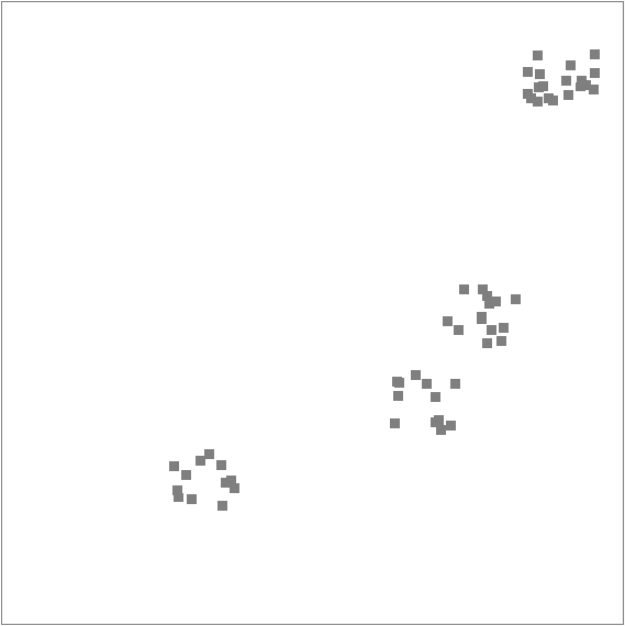
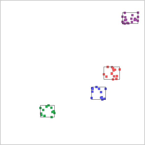
Figure 1: (a) Sample instance with dimension $d=2$ and $n=57$ points, and (b) optimal solution for this instance, with $p=4$ clusters.

Figure 1(a) depicts a sample instance of HRCP in ² (i.e., $d=2$) with $n=57$ points, whereas Figure 1(b) shows a solution for this instance when we are required to identify $p=4$ clusters. The rectangles enclose the four clusters.

Machine Learning techniques are being widely used to understand large amounts of data. The main goal of these techniques is usually to provide a set of rules that can interpret the data and serve as predictive models. These rules are however not always easily explainable to humans. Hyper-rectangular clustering has been proposed as a model for explainable clustering, i.e., a procedure not only providing a partition of the points into clusters but also providing the rationale for the inclusion of each point in its corresponding cluster. Whereas in classical clustering problems the aim is to find a good clustering according to the proposed objective function measuring how good a cluster is, in these novel applications finding such a clustering is not sufficient, e.g., since knowing the reasoning behind the clustering may be more important than the clustering itself (because this could lead to valuable insights on the nature of the data points or because the clustering will be used as a classification method). This issue has been explored in the literature by either developing methods capable of finding both the desired clustering and its “explanating features” (see, e.g., [1, 2, 10]) or developing explanations for existing clusterings (see, e.g., [4, 9]). All these works apply mathematical optimization techniques to these problems, showing that traditional methods from combinatorial optimization can be useful in this setting. In the particular case of hyper-rectangular clustering, it is straightforward to describe the obtained clusters by the bounds defining each hyper-rectangle. Indeed, if each coordinate corresponds to a relevant parameter in the application generating the given points, then clusters are specified by a lower and an upper bound on each parameter, and this is easier to communicate than a distance-based clustering [3].

Several applications of hyper-rectangular clusterings have been explored in the literature (see [8, 11, 14, 15, 13]). In [8] several heuristic procedures are proposed for this problem, and a rectangle-based and graph-based rule learning approach is presented in order to construct a classification method. In [11] a video segmentation and clustering algorithm is presented, and several experiments over video data sets show its effectiveness. In [14] and [15] binary clustering classifying input data into two regions separated by axis-aligned rectangular boundaries is explored, by considering two-cluster solutions in [14] and solutions with an arbitrary but pre-specified number of clusters in [15]. The procedure developed in [14] is applied within an image capturing application. Finally, in [13] a clustering algorithm to discover low and high density regions in multidimensional data is presented, and is applied to data set coming from data mining applications.

Since a clustering is given by a partition of a subset of the input points, the set of feasible solutions is defined in a straightforward way by combinatorial arguments. Furthermore, the objective function (i.e., the total cluster span) is easy to state as a linear expression on natural variables, hence integer programming (IP) techniques are attractive in order to tackle HRCP. The first integer programming approach for hyper-rectangular clustering was proposed in [15], and IP concepts also appear in [14] for $p=2$. A branch-and-cut procedure for the general case was introduced in [12], where an exponential family of valid inequalities was identified and separated with linear programming techniques. The experiments reported therein show that this approach is able to tackle instances of small size within reasonable running times, however, running times are highly impacted when increasing the number $p$ of clusters in the instances.

An extended formulation (i.e., an IP formulation with exponentially-many variables) has been proposed in [6], along with a branch-and-price algorithm to solve the formulation to optimality. The proposed approach outperforms the compact formulation from [12] and is able to handle instances with higher numbers of clusters without degrading the performance. Nevertheless, the size of the instances in terms of the number $n$ of points, which the method can solve to optimality is still small with respect to real-world instances.

In this work we propose an adaptive exact strategy which takes advantage of the capacity to solve small instances to optimality of the previous approaches. Our algorithm starts by solving an instance with a small subset of points and iteratively adds more points if these are not covered by the obtained solution. We prove that as soon as a solution covers the minimum number of points needed for the instance, then the solution is actually an optimal solution for the original problem. We compare the efficiency of the new method against the existing ones with an exhaustive computational experimentation.

2 Formalization of the problem

Given a nonempty set ${\cal X}=\{x^{1},\dots,x^{n}\}$ of $n$ points in $\mathbb{R}^{d}$ and an integer $p\geq 1$, a $p$-clustering of ${\cal X}$ is a collection of subsets $C_{1},\dots,C_{p}\subseteq{\cal X}$, in such a way that ${\cal X}=C_{1}\cup\dots\cup C_{p}$ and $C_{i}\cap C_{j}=\emptyset$ for $i,j\in\{1,\dots,p\}$, $i\neq j$. Each set from $\{C_{i}\}_{i=1}^{p}$ is called a cluster in this context. The span of a cluster $C\subseteq{\cal X}$ over the coordinate $t$ is $\mbox{span}_{t}(C)=\max\{x_{t}:x\in C\}-\min\{x_{t}:x\in C\}$ if $C\neq\emptyset$ and $\mbox{span}_{t}(C)=0$ otherwise, and the total span of $C$ is $\mbox{span}(C)=\sum_{t=1}^{d}\mbox{span}_{t}(C)$. Finally, the total span of a clustering $\mathbb{C}=\{C_{1},\dots,C_{p}\}$ is defined as the sum of the total spans of its constituent clusters, i.e., $\mbox{span}(\mathbb{C})=\sum_{i=1}^{p}\mbox{span}(C_{i})$. The hyper-rectangular clustering problem with axis-parallel clusters (HRCP) consists in determining a $p$-clustering of ${\cal X}$, minimizing the total span.

As we may find in the literature [12], HRCP can be easily formulated by means of mixed integer programming models. For $i\in[n]=\{1,\dots,n\}$ and $c\in[p]=\{1,\dots,p\}$, we consider the binary variable $z_{ic}$ representing whether $x^{i}$ is assigned to the cluster $c$ or not. Also, for $c\in[p]$ and $t\in[d]=\{1,\dots,d\}$, the real variables $l_{tc},r_{tc}\in\mathbb{R}$ represent a lower and an upper bound, respectively, for the points in the cluster $c$ in the coordinate $t$. For $t\in[d]$, we define $\mbox{\rm min}_{t}:=\min\{x_{t}:x\in{\cal X}\}$ and $\mbox{\rm max}_{t}:=\max\{x_{t}:x\in{\cal X}\}$. In this setting, we can formulate the problem as follows.

$$\min \sum_{c=1}^{p}\sum_{t=1}^{d}r_{tc}-l_{tc}$$ (1)

$$\mbox{s.t.}\ \sum_{c=1}^{p}z_{ic} = 1\hskip 46.66249pt\forall i\in[n],$$ (2)

$$l_{tc}+(\mbox{\rm max}_{t}-x^{i}_{t})z_{ic} \leq \mbox{\rm max}_{t}\hskip 28.45274pt\forall i\in[n],c\in[p],t\in[d],$$ (3)

$$r_{tc}+(\mbox{\rm min}_{t}-x^{i}_{t})z_{ic} \geq \mbox{\rm min}_{t}\hskip 30.72902pt\forall i\in[n],c\in[p],t\in[d],$$ (4)

$$l_{tc} \leq r_{tc}\hskip 40.40285pt\forall c\in[p],t\in[d],$$ (5)

$$\mbox{\rm min}_{t}\ \leq\ l_{tc},r_{tc} \leq \mbox{\rm max}_{t}\hskip 28.45274pt\forall c\in[p],t\in[d],$$ (6)

$$z_{ic} \in \{0,1\}\hskip 25.6073pt\forall i\in[n],c\in[p].$$ (7)

The objective function asks to minimize the sum of the total cluster spans. Constraints (2) ask every point to be assigned to one cluster. Constraints (3)-(4) bind the variables, in such a way that $l_{tc}\leq x^{i}_{t}\leq r_{tc}$ if the point $i$ is assigned to the cluster $c$. Constraints (5) avoid bound crossings in empty clusters, whereas constraints (6) impose bounds for the $l$- and the $r$-variables. Finally, constraints (7) specify that the $z$-variables are binary.

The formulation (1)-(7) has obvious symmetry issues (i.e., every clustering admits more than one representation within the model, by renaming the cluster indices), which could be problematic when attempting the solution of this model with general integer programming solvers. This can be tackled by adding symmetry-breaking constraints. Unfortunately, as it is reported in [12], the addition of these does not appear to be effective in practice.

3 The incremental algorithm

Previous exact approaches for HRCP are mostly based on integer programming formulations, as it is the case of formulation (1)-(7) introduced by [12]. Unfortunately, all these approaches can only solve to optimality instances of small size. In this section we propose an adaptive exact strategy which takes advantage of the capacity to solve small instances to optimality of previous approaches.

Our algorithm starts by solving an instance with a small subset of points and iteratively adds more points if these are not covered by the obtained solution. We prove that as soon as a solution covers the whole set of point from the instance, then the solution is indeed an optimal solution for the original problem. Algorithm 1 illustrates the general framework of the proposed methodology. Given a $p$-clustering $\mathbb{C}$ of a subset of points $\hat{\mathcal{X}}\subseteq\mathcal{X}$, we say that $\mathbb{C}$ covers $\mathcal{X}$ if every point $x\in\mathcal{X}$ lies inside at least one of the hyper-rectangles induced by $\mathbb{C}$ (i.e., those enclosing each set of points of the partition). With this definition, the following result allows us to prove the correctness of Algorithm 1.

Algorithm 1 General framework for the incremental algorithm

1:Choose an initial subset of points $\hat{\mathcal{X}}\subseteq\mathcal{X}$

2:Solve the clustering on $\hat{\mathcal{X}}$ and get an optimal solution $\mathbb{C}$

3:if $\mathbb{C}$ covers $\mathcal{X}$ then

4:     Add each point $x\in\mathcal{X}\setminus\hat{\mathcal{X}}$ to the cluster from $\mathbb{C}$ enclosing $x$

5:     return $\mathbb{C}$

6:else

7:     Add to $\hat{\mathcal{X}}$ some points from $\mathcal{X}\setminus\hat{\mathcal{X}}$

8:     go to Line 2

Lemma 1.

Let $\hat{\mathcal{X}}\subseteq\mathcal{X}$ be a subset of points and $\mathbb{C}$ an optimal $p$-clustering of $\hat{\mathcal{X}}$ (i.e., with minimum total span). If $\mathbb{C}$ covers $\mathcal{X}$, then it represents an optimal $p$-clustering for $\mathcal{X}$.

Proof.

Since $\mathbb{C}$ covers $\mathcal{X}$, we can add each point of $\mathcal{X}\setminus\hat{\mathcal{X}}$ to some cluster from $\mathbb{C}$, thus yielding a feasible $p$-clustering for $\mathcal{X}$ without changing the hyper-rectangles induced by the clustering (i.e., with a total span equal to $\mbox{span}(\mathbb{C})$). Assume there exists another $p$-clustering $\mathbb{C}^{\prime}$ of $\mathcal{X}$ with $\mbox{span}(\mathbb{C}^{\prime})<\mbox{span}(\mathbb{C})$. Since $\mathbb{C}^{\prime}$ is a $p$-clustering of $\mathcal{X}$, it also covers $\hat{\mathcal{X}}$, thus contradicting the fact of $\mathbb{C}$ being optimal for $\hat{X}$. ∎

An alternative proof for Lemma 1 follows from the fact that HRCP over $\hat{\mathcal{X}}$ is indeed a combinatorial relaxation of HRCP over $\mathcal{X}$, as it allows points from $\mathcal{X}\setminus\hat{\mathcal{X}}$ to be left uncovered by the solution. More precisely, it is trivial to see that every feasible solution for HRCP over $\mathcal{X}$ gives also a feasible solution for HRCP over $\hat{\mathcal{X}}$. Hence, if an optimal solution for $\hat{\mathcal{X}}$ (i.e., the relaxation) is also feasible for $\mathcal{X}$ (i.e., the original problem), then this solution is indeed optimal for $\mathcal{X}$. Remark 1 follows from this fact.

Remark 1.

Any lower bound for HRCP over $\hat{\mathcal{X}}\subseteq\mathcal{X}$ is a valid lower bound for HRCP over $\mathcal{X}$.

Proposition 1.

Algorithm 1 always finds an optimal solution for HRCP over $\mathcal{X}$.

Proof.

The algorithm finishes only when the condition on Line 3 is satisfied, i.e., when $\mathbb{C}$ covers $\mathcal{X}$. By Lemma 1, this provides an optimal solution for HRCP over $\mathcal{X}$, since $\mathbb{C}$ is an optimal $p$-clustering of $\hat{\mathcal{X}}\subseteq\mathcal{X}$. So it just remains to prove that the algorithm reaches this point at least once.

The set $\hat{\mathcal{X}}$ is increased on every iteration by adding to it points from $\mathcal{X}\setminus\hat{\mathcal{X}}$, hence the algorithm will iterate until $\hat{\mathcal{X}}=\mathcal{X}$, if it does not finish earlier. At this point, the clustering $\mathbb{C}$ obtained in Line 2 does trivially cover $\mathcal{X}$, hence it is returned (as it is optimal) in Line 5. ∎

A strong characteristic of Algorithm 1 is the fact that as soon as a feasible solution for $\mathcal{X}$ is found (i.e., in Step 3), the algorithm stops as this solution is optimal. On the other hand, if the process is stopped before its termination (e.g., due to an imposed time limit), no feasible solution (even if sub-optimal) can be returned. To tackle this issue, we may profit from the several executions of Step 2 which tries to find optimal solutions for HRCP over $\hat{\mathcal{X}}$. During this process, the procedure may generate intermediate solutions ($p$-clusterings) that are feasible for $\hat{\mathcal{X}}$ (for example, sub-optimal incumbent solutions during the branch-and-bound process when solving Step 2 using a MIP solver). Even if the optimal solution on this step does not provide a cover for $\mathcal{X}$, these intermediate solutions may do. Therefore, we can check these solutions searching for feasible solutions for HRCP over $\mathcal{X}$, thus keeping track of an incumbent (i.e., the current best feasible solution found) in Algorithm 1.

Remark 2.

Any feasible solution for $\hat{\mathcal{X}}$ found during Step 2 may represent a feasible solution for the original instance $\mathcal{X}$ and may help to improve the incumbent, which in turn gives an upper bound for the problem.

By Remark 1, any lower bound for HRCP over $\hat{\mathcal{X}}$ obtained on Step 2 can be used as a lower bound for HRCP over $\mathcal{X}$. In addition, by using the upper bound described in Remark 2, Algorithm 1 can keep track of the optimality gap at any time. This gap can be closed even if the solution $\mathbb{C}$ found in Step 2 is not feasible for $\mathcal{X}$ (i.e., the incumbent from previous iterations may be proved to be optimal even if it does not match with $\mathbb{C}$). These additions can be included in the algorithm, thus generating the procedure described in Algorithm 2.

Algorithm 2 The complete incremental algorithm

1:Choose a an initial subset of points $\hat{\mathcal{X}}\subseteq\mathcal{X}$

2:LB $\leftarrow$ 0, UB $\leftarrow$ $+\infty$, incumbent $\leftarrow$ null

3:while LB $<$ UB do

4:     Solve the clustering on $\hat{\mathcal{X}}$ and get solution $\mathbb{C}$

5:     if $\mathbb{C}$ covers $\mathcal{X}$ then

6:         Add each point $x\in\mathcal{X}\setminus\hat{\mathcal{X}}$ to a cluster from $\mathbb{C}$ enclosing $x$

7:         return $\mathbb{C}$

8:     else

9:         LB $\leftarrow$ max(LB, lower bound from Line 4)

10:         for each feasible solution $\mathbb{C}^{\prime}$ found at Line 4 do

11:              if $\mathbb{C}^{\prime}$ covers $\mathcal{X}$ and is better than incumbent then

12:                  Update UB and incumbent with $\mathbb{C}^{\prime}$                        

13:         Add to $\hat{\mathcal{X}}$ some points from $\mathcal{X}\setminus\hat{\mathcal{X}}$      

14:return incumbent

3.1 Sampling metrics

Lines 1 and 13 from Algorithm 2 add new points to $\hat{\mathcal{X}}$, by performing a sampling of the points in $\mathcal{X}\backslash\hat{\mathcal{X}}$. We refer to these lines as the initialization and expansion steps, respectively. These steps can be performed in many different ways.

The most straightforward sampling method is a random sampling. For the initialization step, we may set $\bar{\mathcal{X}}$ to a random sample, e.g., by uniformly choosing points from $\mathcal{X}$ with some fixed probability. The same can be done for the expansion step, choosing points from $\mathcal{X}\setminus\mathcal{X}$ which are not covered by $\mathbb{C}$. Unfortunately, although not unexpected, preliminary experimentation proved this method to be inefficient in practice. A random sampling tends to conserve the spatial distribution of the data points, however, the best sampling method should be able to identify the points which are most likely to lie in the perimeter of one of the hyper-rectangle which encloses a cluster in the solution, as these are the points “defining” the solution. Figure 2 shows a small example in ² illustrating the difference between a uniform random sample (left) and a sample which identifies points which are most likely to lie in the borders of the hyper-rectangles defining the optimal solution (right). Black points represent the sample $\hat{\mathcal{X}}$ and gray points are the remaining points $\mathcal{X}\setminus\hat{\mathcal{X}}$.

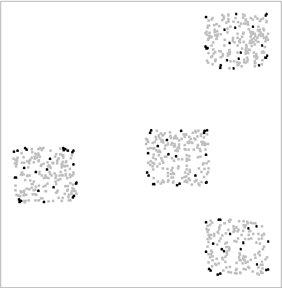
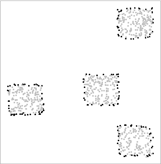
Figure 2: A small example in ² illustrating the difference between a uniform random sample (left) and a sample which identifies points which are most likely to lie in the borders of the hyper-rectangles defining the optimal solution (right). Black points represent the sample $\hat{\mathcal{X}}$ and gray points are the remaining points $\mathcal{X}\setminus\hat{\mathcal{X}}$.

In this section we explore different sampling approaches and propose different alternatives to perform these sampling steps, thus obtaining different versions of the algorithm. Throughout the remainder of this work, let $N:\mathcal{X}\rightarrow 2^{\mathcal{X}}$ be any neighbourhood function on $\mathcal{X}$. In particular, we will use $N(x)=\{y\in\mathcal{X}\setminus\{x\}:\|x-y\|_{2}\leq\delta\}$, for a fixed value of $\delta\in_{+}$, however, every method proposed in this paper can be applied for other neighbourhood functions.

3.1.1 Neighbourhood metric

Identifying points in the border of a cluster is similar to the classical DBSCAN algorithm [7] for density-based clustering, so we use its notion of core and border points. In this classical method, a value $minPts\in\mathbb{N}$ is chosen, and a point $x\in\mathcal{X}$ having $|N(x)|\geq minPts$ is called a core point, and it is considered to have high chances of lying completely in the interior of the cluster which contains it. In other words, this point is very likely to not lie in the border of the cluster. All points that are not core points are defined to be border points. The algorithm proposed in the referenced work applies a heuristic which collects core points in a smart way in order to detect the clusters in the solution.

Even when the notions of border and core points may be useful in our setting, we further need something slightly more flexible than fixing a value $minPts$ to determine border points, as we need to refine this decision in the subsequent iterations of Algorithm 2. Nevertheless, we observe that when points in a cluster are uniformly distributed in the space, the number of neighbours of a point $x\in\mathcal{X}$ is gradually reduced when the point is close to the border of the cluster, and is minimal for the points lying in the border. Hence, we propose to use $|N(x)|$ as an (inverse) measure of how likely is a point to be in the border of its cluster. We denote this metric as the neighbourhood metric and we use it as follows:

• Initialization step: Let $x_{0}\in\mathcal{X}$ be a point with minimum value for $|N(x_{0})|$. Set $\hat{X}=\{x\in\mathcal{X}:|N(x)|\leq\alpha|N(x_{0})|\}$, for a given $\alpha\geq 1$.

• Increment step: Sort points $\mathcal{X}\setminus\hat{\mathcal{X}}$ which are not covered by the obtained solution $\mathbb{C}$, and choose those with fewer neighbors, up to a limit of $k\in\mathbb{N}$ points.

3.1.2 Eccentricity metric

The neighbourhood metric proposed in Section 3.1.1 may not be very accurate identifying border points when different clusters have different densities; a border point from a very dense cluster may have more neighbours than a core point from a cluster with low density. To tackle this issue, we propose a metric which considers the position of a point relative to the position of its neighbours, considering that border points have usually every neighbour towards the center of the cluster.

For a given coordinate $t\in[d]$, we define the lower and upper neighbourhoods of a point $x\in\mathcal{X}$ in dimension $t$ as $N^{-}_{t}(x)=\{y\in N(x):y_{t}\leq x_{t}\}$ and $N^{+}_{t}(x)=\{y\in N(x):y_{t}>x_{t}\}$, respectively.

Definition 1.

The eccentricity of a point $x\in\mathcal{X}$ (with $|N(x)|>0$) in dimension $t\in[d]$ is

$$E^{t}(x)=\frac{\max\{|N^{-}_{t}(x)|,|N^{+}_{t}(x)|\}}{|N(x)|}$$ (8)

and its global eccentricity is $E(x)=\max_{t\in[d]}\{E^{t}(x)\}$. If $|N(x)|=0$ then $E^{t}(x)=1$.

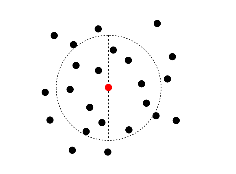
$E^{1}(x)=\frac{6}{11}\approx 0.55$

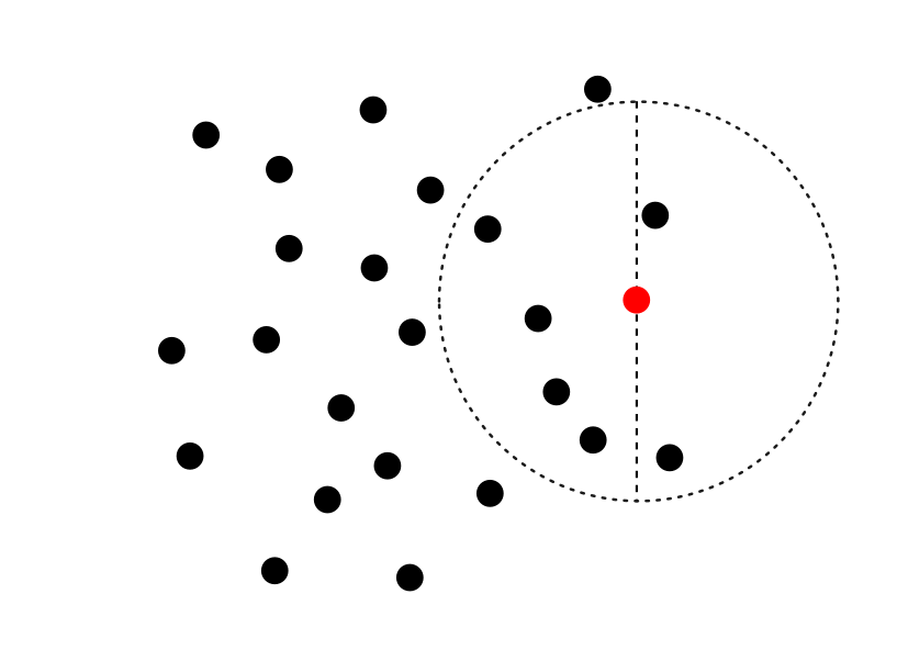
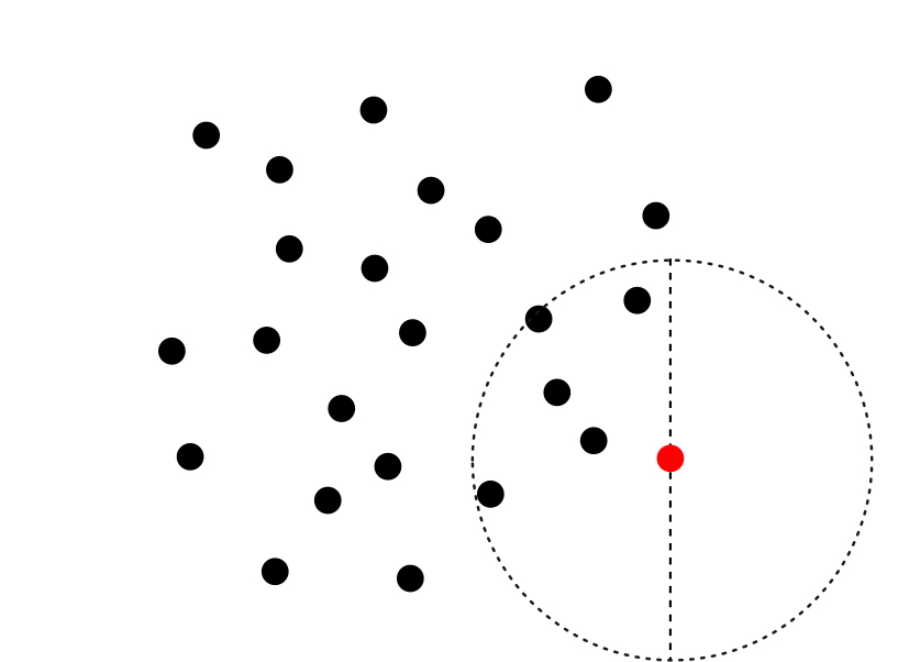
  $E^{1}(x)=\frac{4}{6}\approx 0.67$   $E^{1}(x)=\frac{5}{5}=1$

Figure 3: Eccentricity (fixed on the horizontal coordinate, $t=1$ in the example) of different points in a cluster as the points are taken closer to the border of the cluster.

Figure 3 depicts the the eccentricity (fixed on the horizontal coordinate, $t=1$ in the example) of different points in a cluster as the points are taken closer to the border of the cluster. The point chosen on the first case (left) is a very centric point and has an eccentricity of $E^{1}(x)=\frac{6}{11}\approx 0.55$. The second example (middle) is closer to the border and its eccentricity is $E^{1}(x)=\frac{4}{6}\approx 0.67$. Finally, the third example (right) lies in the border of the cluster, and its eccentricity is $E^{1}(x)=\frac{5}{5}=1$. The eccentricity of any point is a value between 0.5 and 1, regardless of the density of the clusters and the chosen neighbourhood function $N$. The eccentricity metric for Algorithm 2 works as follows:

• Initialization step: Let $x_{0}\in\mathcal{X}$ be a point with maximum global eccentricity $E(x_{0})$. Set $\hat{X}=\{x\in\mathcal{X}:E(x)\geq\beta E(x_{0})\}$, for a given $\beta\in[0,1]$.

• Increment step: Sort points $\mathcal{X}\setminus\hat{\mathcal{X}}$ which are not covered by the obtained solution $\mathbb{C}$, and choose those with higher global eccentricity, up to a limit of $k\in\mathbb{N}$ points.

3.1.3 Distance-Eccentricity metrics

Although the eccentricity metric might properly deal with issues caused by the presence of clusters with different densities, both this and the neighbourhood metrics suffer from another issue, related to the distance between clusters. Figure 4 shows an example in which a point in the border of a cluster is not detected either by the neighbour metric nor by the eccentricity metric. This example shows the importance of the definition of $N(x)$ and its impact on these metrics (e.g., a bad choice of the parameter $\delta$ defining the size of the neighbourhood when clusters are not much separated).

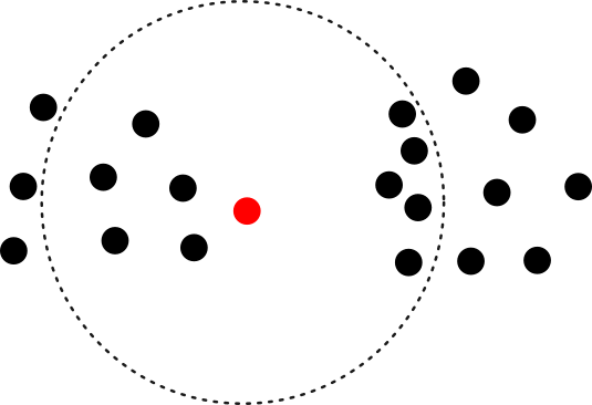
$|N(x)|$ is high $\Rightarrow$ neighbour metric fails

$E(x)$ is low $\Rightarrow$ eccentricity metric fails

Figure 4: Example in which a point which lies in the border of a cluster is not detected either by the neighbour metric nor by the eccentricity metric.

With the goal of dealing with this type of situations, we propose another metric which considers not only the number of neighbours on “each side” but also the average distance to them. More precisely, a candidate point for being a border point is a point in which the distance to the points in one side of its neighbourhood is very different to the distance to the other side. We formalize this concept in the following definition.

Definition 2.

The distance-eccentricity of a point $x\in\mathcal{X}$ in dimension $t\in[d]$ is

$$D^{t}(x)=|\text{dist}_{t}(x,N^{-}_{t}(x))-\text{dist}_{t}(x,N^{+}_{t}(x))|,$$ (9)

where $\text{dist}_{t}(x,X)=\frac{1}{|X|}\sum_{y\in X}\|y_{t}-x_{t}\|_{2}$ is the average distance between $x$ and $X\subseteq\mathcal{X}$ on coordinate $t\in[d]$. The global distance-eccentricity is $D(x)=\max_{t\in[d]}\{D^{t}(x)\}$.

The distance-eccentricity metric for Algorithm 2 works analogously to the eccentricity metric:

• Initialization step: Let $x_{0}\in\mathcal{X}$ be a point with maximum global distance-eccentricity $D(x_{0})$. Set $\hat{X}=\{x\in\mathcal{X}:D(x)\geq\beta D(x_{0})\}$, for a given $\beta\in[0,1]$.

• Increment step: Sort points $\mathcal{X}\setminus\hat{\mathcal{X}}$ which are not covered by the obtained solution $\mathbb{C}$, and choose those with higher global distance-eccentricity, up to a limit of $k\in\mathbb{N}$ points.

We conclude this section noting that none of the metrics introduced in this work depend on the current elements in the set $\hat{\mathcal{X}}$. Therefore, the values required by these metrics can be computed at the beginning of the algorithm with almost no impact on its performance.

4 Computational experimentation

We report in this section our computational experience with the incremental algorithm presented in Section 3 and using the different alternative sampling metrics from Section 3.1. For the solution of HRCP over the subset of points $\hat{\mathcal{X}}$ (Line 4 of Algorithm 2) we use the compact formulation (1)–(7), proposed in [12]. We implemented the procedure in Java using Cplex as the integer programming solver for formulation (1)–(7), interfacing with Cplex by resorting to the Concert API [5]. The source code of our implementation is available online.

In order to conduct experiments with controlled instances having predictable optima, we use the instance generator introduced in [12] for the experiments. This procedure takes as input the dimension $d$, the number $n$ of points to be generated, the number $p$ of clusters to generate, and a parameter $s\in[0,1]$ specifying the dispersion for the generated clusters. A set of $p$ originating points is randomly generated with uniform distribution in $[-1,1]^{d}$, which will act as the originating points for the clusters. Afterwards, the $p$ clusters are generated by randomly constructing $n-q$ points around the originating points with uniform distribution and span $s$. To this end, an originating point $\bar{x}$ is randomly chosen and a point in $\bar{x}+[-s/2,s/2]^{d}$ selected with uniform distribution is added to the instance.

In our experimentation we compare the compact formulation (1)–(7) solved directly with Cplex (denoted as CMP) and the incremental algorithm by using three different sampling metrics: neighbouring, eccentricity and distance-eccentricity (denoted as NM, EM and DM, respectively). We impose a time limit of 1800 seconds to the solver.

Figure 5 depicts the processing times on instances in ³ with $p=4$ clusters, ranging $|\mathcal{X}|$ from 40 to 1000 points. In the picture, we can clearly verify that running times of CMP are highly impacted by the number of points in the instances, contrary to the incremental algorithm, which can solve instances with 1000 points in less than 2 minutes. Indeed, for instances of 400 points CMP takes on average more than 500 seconds while DM needs less than 100 seconds to solve instances of up to 1000 points (and similarly for NM and EM). We observe that running times of DM tend to be slightly smaller than those of NM and EM, specially on harder instances.

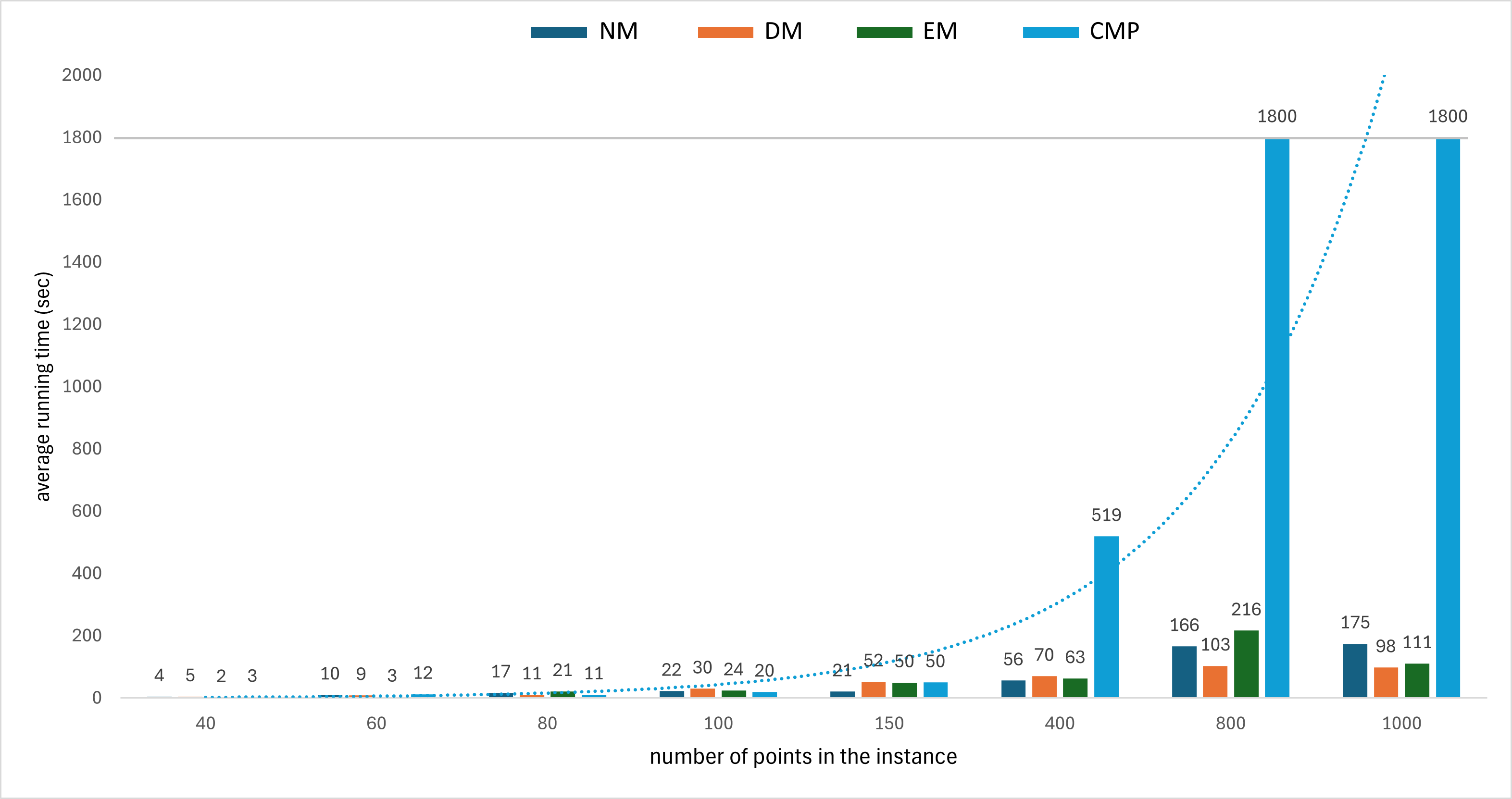
Figure 5: Processing times on instances in ³ with $p=4$ clusters, ranging from 40 to 1000 points.

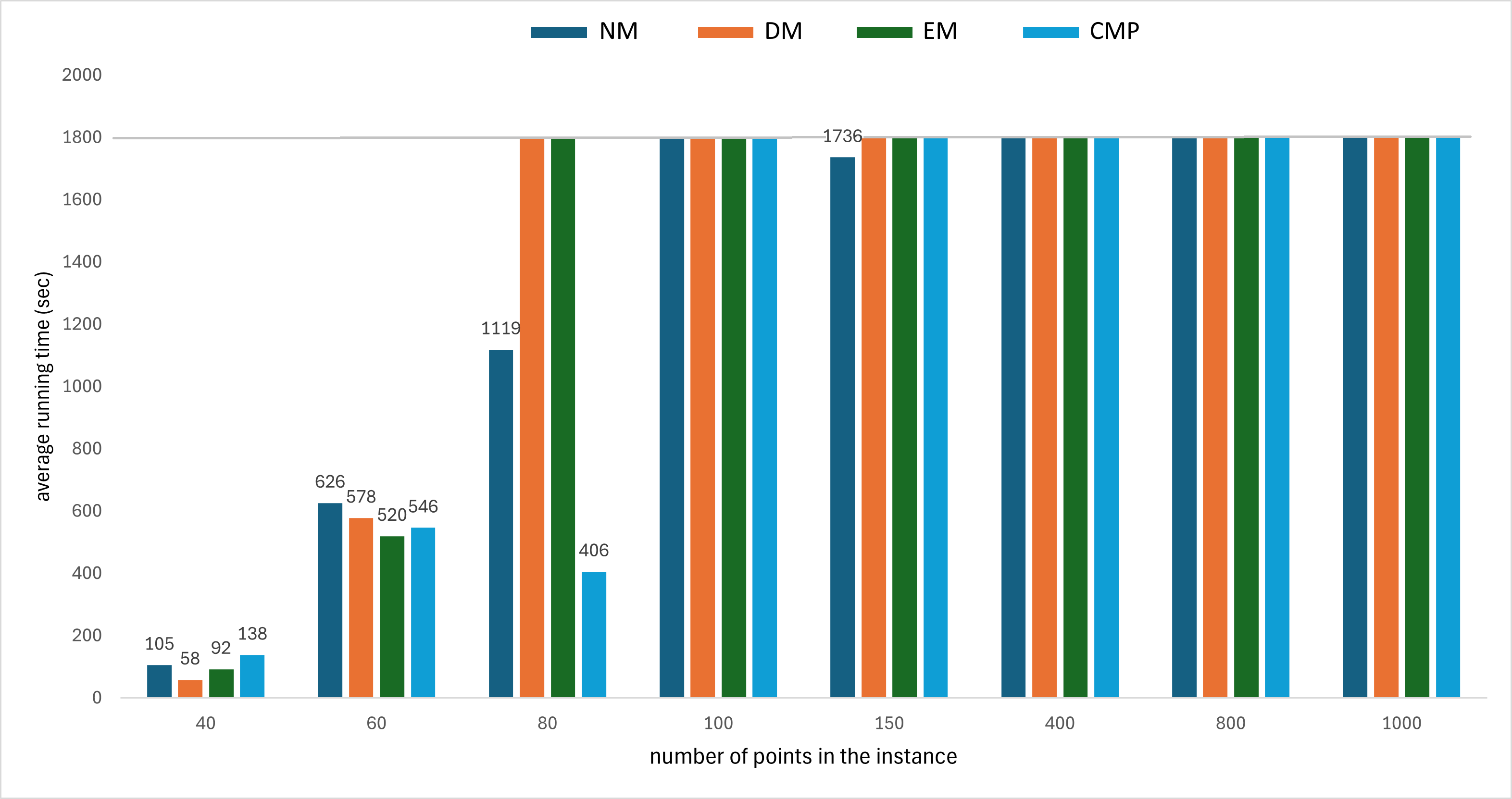
Figure 6: Processing times on instances in ³ with $p=6$ clusters, ranging from 40 to 1000 points.

Unfortunately, the running times of all methods are highly impacted by increasing the number of clusters in the instances. Figure 6 depicts the processing times on instances in ³ with $p=6$ clusters; the picture shows that all methods reach the time limit even for instances of 100 points. However, when we analyze the obtained (suboptimal) solutions provided by the methods, we observe that the optimality gaps achieved by the incremental algorithm are significantly better than those provided by CMP. Figure 7 depicts these gaps in the same set of instances; the gap is calculated as $(sol-lb)/lb$, where $sol$ is the span of the obtained clustering and $lb$ is the best lower bound found by the method. For instances with 200 points, CMP achieves optimality gaps of around 46% and for bigger instances the gaps surpass 100%, sometimes reaching almost 140% in our test set. On the other hand, the incremental algorithm achieves very small gaps, notably providing solutions with an optimality gap of around 2% for instances of 1000 points. Again, DM seems to provide better solutions than NM and EM.

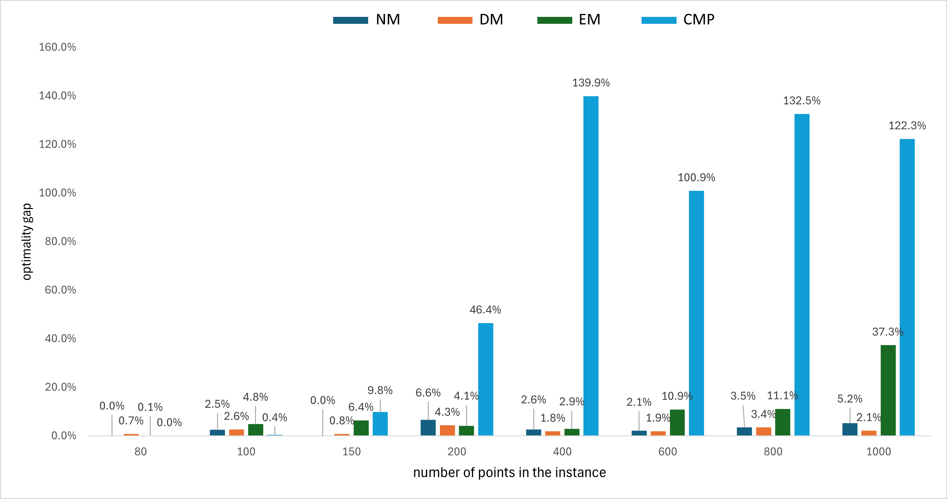
Figure 7: Optimality gaps on instances in ³ with $p=6$ clusters, ranging from 40 to 1000 points.

We conclude this section analyzing two interesting aspects of the incremental algorithm: the number of points needed to find an optimal solution (i.e., the size of $\hat{\mathcal{X}}$ at the end of the execution) and the number of iterations performed by the method (i.e., the number of times the increment step is called in order to add points to $\hat{\mathcal{X}}$). These two key aspects allows us to better understand the incremental algorithm independently from the model and/or solver used to obtain the intermediate solutions for HRCP over $\hat{\mathcal{X}}$ (Line 4 of Algorithm 2). The number of points in $\hat{\mathcal{X}}$ gives an idea of the size of the subproblems that we need to solve and the number of iterations points out how many of these subproblems will be needed to be solved. These values altogether give an idea of the scalability of the proposed method and may suggest which type of model and/or solver would be more suitable to use for the subproblems. We focus on the set of instances analyzed on Figure 5, i.e., instances in ³ with $p=4$ clusters.

Figure 8 shows the percentage of points from the original instance that are actually needed to find the optimal solution, i.e., the size of $\hat{\mathcal{X}}$ with respect to the size of $\mathcal{X}$, at the end of the execution. For larger instances, the percentage of needed points is significantly smaller. In particular, for instances of 1000 points, the incremental algorithm (with both DM and NM metrics) needs to use less than 10% of these points. Although, the EM alternative seems to need almost twice the points used by DM and NM, we will see that this alternative needs less iterations in general.

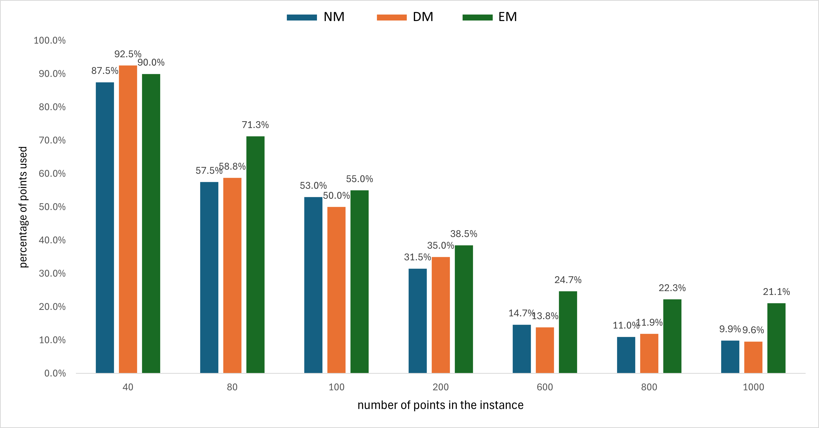
Figure 8: Number of points on $\hat{\mathcal{X}}$ at the end of the execution of the incremental algorithm on instances in ³ with $p=4$ clusters, ranging from 40 to 1000 points.

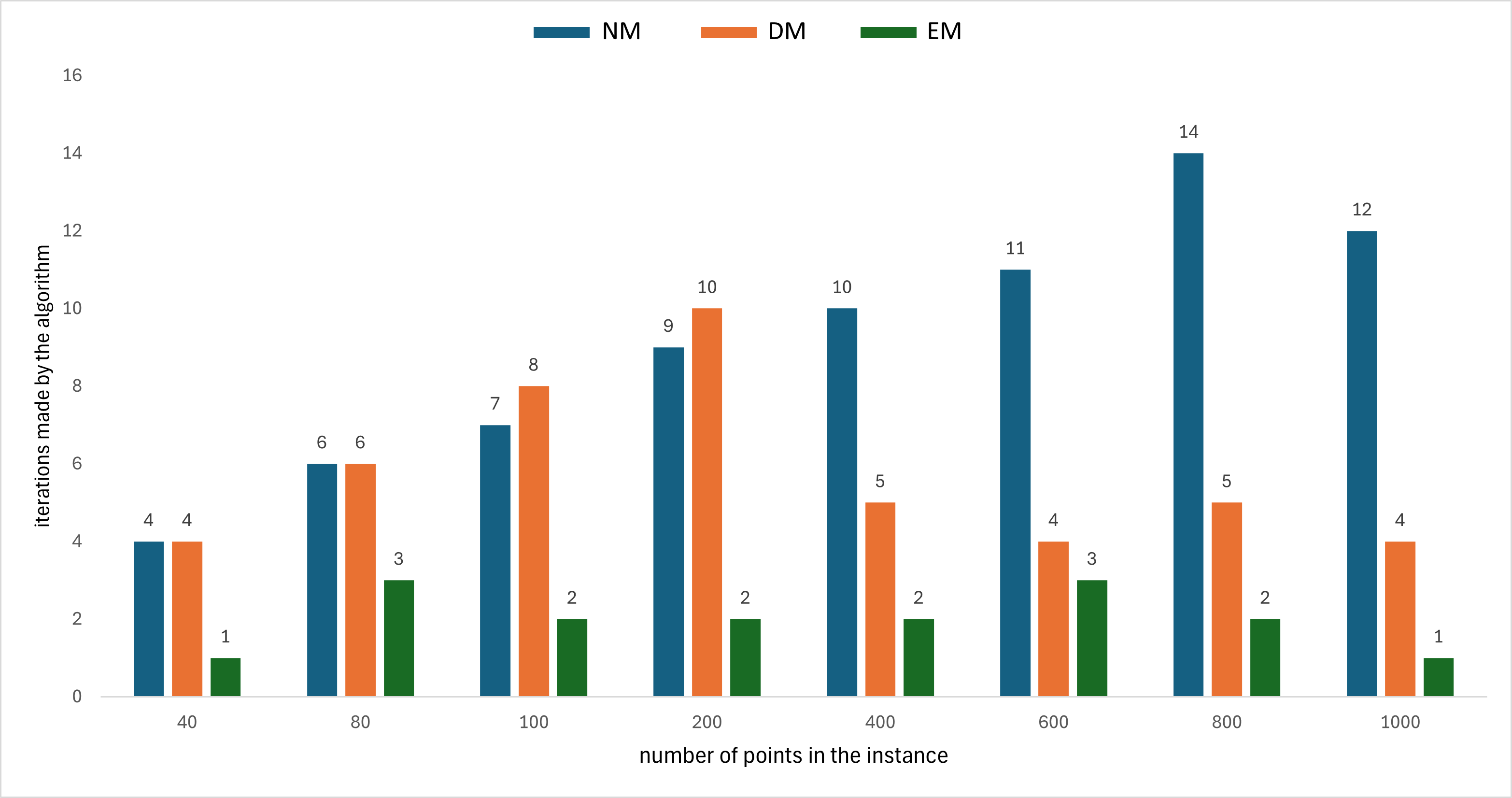
Figure 9: Number of iterations made by the incremental algorithm on instances in ³ with $p=4$ clusters, ranging from 40 to 1000 points.

Figure 9 shows the number of iterations needed by the algorithm to solve the instances, i.e., the number of times the increment step is called in order to add points to $\hat{\mathcal{X}}$. The picture shows the effectiveness of the sampling performed by EM, as this method needs very few iterations to find an optimal solution; three iterations in the worst case and only one iteration for the largest-sized instances. This characteristic of EM balances the fact that this variant uses more points than the others for the final $\hat{\mathcal{X}}$. When contrasting the number of iterations needed by NM and DM, we can see that DM seems to need less than NM, thus breaking to tie that we saw between these two methods with respect to the number of needed points.

Overall, we can say that none of the alternatives among NM, EM and DM, completely dominates the others. However, if it is desirable to solve the least number of subproblems, EM seems to be the better option, while DM seems to be the better fit if the size of the subproblems is to be minimized. Also, as we have seen at the beginning of this section, DM tends to slightly outperform the other two variants in terms of running times and optimality gaps.

5 Conclusions and further remarks

In this work we have proposed an incremental adaptive exact approach for the hyper-rectangular clustering problem with axis-parallel clusters (HRCP). Previous exact approaches for HRCP are mainly based on solving integer programming formulations, but the size of the instances in terms of the number of points, which the method can solve to optimality was still small with respect to real-world instances. Our proposed approach takes advantage of the capacity to solve small instances to optimality of the previous approaches and it proves to be able to solve instances with significantly larger sizes, in terms of number of points to be clustered.

We proposed several sampling metrics to be used by the algorithm: neighbour (NM), eccentricity (EM) and distance-eccentricity (DM) metrics. Although none of these alternatives completely dominates the others, each of them has different characteristics which could be exploited. For example, if it is desirable to solve the least number of subproblems, EM seems to be the better option, while DM seems to be the better fit if the size of the subproblems is to be minimized. Also, DM tends to slightly outperform the other two variants in terms of running times and optimality gaps.

Although there seems to be several ways to improve the proposed algorithm, our computational results show that the proposed approach allows to make progress in terms of scalability at solving this problem to optimality. There exist several lines of future research including, e.g., the exploration of other sampling metrics, alternative models for the subproblem, and the posibility of removing points from the subproblems (in contrast to only adding points during the overall procedure).

References

- [1] Benati, S., Ponce, D., Puerto, J., and Rodríguez-Chía, A. M. A branch-and-price procedure for clustering data that are graph connected. European Journal of Operational Research 297, 3 (2022), 817–830.
- [2] Bertsimas, D., Orfanoudaki, A., and Wiberg, H. Interpretable clustering: an optimization approach. Machine Learning 110 (2021), 89–138.
- [3] Bhatia, A., Garg, V., Haves, P., and Pudi, V. Explainable clustering using hyper-rectangles for building energy simulation data. IOP Conference Series: Earth and Environmental Science 238, 1 (feb 2019), 012068.
- [4] Carrizosa, E., Kurishchenko, K., Marín, A., and Romero Morales, D. On clustering and interpreting with rules by means of mathematical optimization. Computers & Operations Research 154 (2023), 106180.
- [5] Cplex, IBM ILOG. User’s manual for cplex. International Business Machines Corporation (2022).
- [6] Delle Donne, D., and Marenco, J. A branch-and-price algorithm for the hyper-rectangular clustering problem with axis-parallel clusters and outliers. In 25ème Congrès de la ROADEF 2024 (2024).
- [7] Ester, M., Kriegel, H.-P., Sander, J., Xu, X., et al. A density-based algorithm for discovering clusters in large spatial databases with noise. In Knowledge Discovery and Data Mining (1996), vol. 96, pp. 226–231.
- [8] Gao, B. J. Hyper-rectangle-based discriminative data generalization and applications in data mining. Phd thesis, Simon Fraser University, 2007.
- [9] Lawless, C., and Günlük, O. Cluster explanation via polyhedral descriptions. In International Conference on Machine Learning (2023), pp. 18652–18666.
- [10] Lawless, C., and Günlük, O. Fair minimum representation clustering. In Integration of Constraint Programming, Artificial Intelligence, and Operations Research (Cham, 2024), B. Dilkina, Ed., Springer Nature Switzerland, pp. 20–37.
- [11] Lee, S.-L., and Chung, C.-W. Hyper-rectangle based segmentation and clustering of large video data sets. Information Sciences 141, 1 (2002), 139–168. Intelligent Multimedia Computing and Networking.
- [12] Marenco, J. An integer programming approach for the hyper-rectangular clustering problem with axis-parallel clusters and outliers. Discrete Applied Mathematics 341 (2023), 180–195.
- [13] Ordóñez, C., Omiecinski, E. R., Navathe, S. B., and Ezquerra, N. A clustering algorithm to discover low and high density hyper-rectangles in subspaces of multidimensional data. Technical Report GIT-CC-99-20, Georgia Institute of Technology, 1999.
- [14] Park, S. H. Classification with axis-aligned rectangular boundaries. In Cross-Disciplinary Applications of Artificial Intelligence and Pattern Recognition (2012), V. K. Mago and N. Bhatia, Eds.
- [15] Park, S. H., and Kim, J.-Y. Unsupervised clustering with axis-aligned rectangular regions. Technical report, Stanford University, 2009.