Majorized Bayesian Persuasion and Fair Selection
Abstract
We address the fundamental problem of selection under uncertainty by modeling it from the perspective of Bayesian persuasion. In our model, a decision maker with imperfect information always selects the option with the highest expected value. We seek to achieve fairness among the options by revealing additional information to the decision maker and hence influencing its subsequent selection. To measure fairness, we adopt the notion of majorization, aiming at simultaneously approximately maximizing all symmetric, monotone, concave functions over the utilities of the options. As our main result, we design a novel information revelation policy that achieves a logarithmic-approximation to majorization in polynomial time. On the other hand, no policy, regardless of its running time, can achieve a constant-approximation to majorization. Our work is the first non-trivial majorization result in the Bayesian persuasion literature with multi-dimensional information sets.
toc
1 Introduction
Selection problems arise in hiring decisions, college admissions, ad auctions, and many other scenarios. Typically, a selection process involves defining an explainable selection rule that solves an optimization problem over the agents (e.g., applicants or advertisers). Perhaps the simplest and most common rule is to choose the best or most qualified agent(s) – for example, many countries use standardized test scores for college admissions. Under natural simplifying assumptions, such a meritocratic rule will maximize the utilitarian social welfare, and can be perceived as fair. Nevertheless, its outcomes may not always align with other fairness considerations. For instance, one can adopt the view of max-min fairness and aim at helping the worst-off agent.
The meritocratic rule has a perhaps more subtle issue: when trying to evaluate the agents and define the “best” one, the quality measurements may be imperfect. Indeed, the decision maker uses observable information or features of the agents to reach a decision, but counterfactually, a different decision could have been made in the presence of more certain or complete information. This issue can have disproportionate negative impacts on certain demographic groups and therefore undermine fairness perceptions towards the rule. To address the issue, there has been a long line of recent research focusing on modeling this uncertainty and constructing randomized selection policies to achieve fair outcomes [KR18, CMV20, SKJ21, SWZ+23, DKKS24]. As a practical example, in many hiring situations, the interviewers are required to interview at least a certain number of candidates from prespecified demographic groups, as an attempt to mitigate the impact of such uncertainty and to achieve fairness.
Fairness via Information Revelation.
We diverge from this line of research and take a view inspired by the influential Bayesian persuasion literature, starting with the seminal work of Kamenica and Gentzkow [KG11]. We ask:
Given uncertainty about agent qualities, how much additional information should be gleaned and revealed to the decision maker (either by the agents themselves or by a central entity), so that even if the decision maker sticks to “selecting the best”, it still yields a fair outcome to the agents?
To approach this high-level question, we use the following model. (See Au and Kawai [AK20] for a related model.) Each agent has an uncertain scalar quality, and its true quality is known to an entity – either the agent itself or an intermediary. This entity then signals additional information independently for each agent to the decision maker to refine its uncertainty via Bayes’ rule. Analogous to [AK20], this signaling process can be done in a distributed fashion by the agents themselves, a property that is often desirable for the applications we consider in order to preserve privacy of agents’ true quality. Subsequently, it can happen that several agents have comparable posterior quality in the eyes of the decision maker, and a fair selection can be made by the decision maker without significantly sacrificing its own optimality notion of selecting the posterior best.
As a concrete motivation, consider designing a standardized form for admission or hiring. The form is the signaling scheme - it is designed centrally by the decision maker, filled separately by agents, and the decision maker can break ties based on information revealed in the forms, sometimes in conjunction with a lottery number assigned to each agent, to ensure fairness in selection. We present the formal model in Section 2, and an example in Example 2.4.
In order to define fairness, we consider the vector of expected utilities received by the agents, where each agent receives utility equal to its true value if it is selected. We seek signaling (or information revelation) policies whose utility vector is approximately majorized [HLP34, GMP05, KK06, CS19], meaning that all symmetric, monotone, concave functions over the utilities are simultaneously approximately maximized by the same policy. Such fairness functions capture, for instance, max-min fairness (maximizing the minimum utility) and the Nash welfare (maximizing the geometric mean of the utilities).
At one extreme, if the agents do not reveal any additional information, the agent with the highest expected quality, according to the decision maker’s prior, is selected. As mentioned before, this can be problematic in terms of fairness to counterfactual information. We show in Example 2.7 that the other extreme – where each agent reveals its exact quality (Full Revelation) – may be far from fair as well, even when the qualities only take “high”, “medium”, and “low” values. This example highlights the need to carefully choose which information to reveal.
We note that such information revelation considerations extend beyond the motivating settings described above. As an example, consider a government agency (the decision maker) that has fixed rules for allocating money designated to a social welfare cause such as refugee resettlement. Local agencies typically are better informed about welfare needs of the groups they serve, and can selectively reveal information in order to facilitate fairness for these groups.
Summary of Results.
We present a detailed summary of our results in Section 2 after we present our formal model. Informally, our main result is a novel set of signaling (or information revelation) mechanisms that achieve approximate majorization. (See Theorem 2.8.) The key technical hurdle with designing such policies is the behavior of the decision maker – this decision maker chooses the best (or approximately best) agent given its information. For any given fairness objective (such as max-min fairness), a general algorithmic result due to Dughmi and Xu [DX16] yields an FPTAS for any Bayesian persuasion problem with arbitrary information sets, assuming that the sender can correlate agent signals. However, such a generic approach does not shed light on the existence of policies that simultaneously approximate any fairness objective, and this fact requires us to unearth specific structure in our problem.
Our main contribution in Section 4 is in unearthing such structure for the selection problem via a novel class of signaling policies with simple structure, leading to positive existence and computational results for approximately majorized policies. We term the novel set of policies as Single Mean, and these generate, in a randomized fashion, information signals where the posterior inferred by the decision maker maps the agents’ values to a common mean quality. This mapping to the common mean happens with as large a probability as possible, hence giving the decision maker wide leeway in implementing a fair selection even when it “goes with the best”. Though this policy sounds intuitive, its analysis is far from obvious as we discuss below. Informally, the final result is a polynomial-time-computable and -approximately majorized policy111Our results are bicriteria, and assume the societal decision maker is a -approximate welfare maximizer., where is the ratio of the largest to smallest quality value. This means for any fairness function, the policy yields an -approximation in polynomial time.
As a corollary, our work also presents an approximation algorithm for any given fairness function when agents generate signals independently of other agents. As shown in Section 4.4, our results easily extend to handle the case where the agents’ utility (on which we seek to be fair) is different from their quality (whose posterior is used by the social planner to perform allocation). We note that the FPTAS for general Bayesian persuasion in [DX16] assumes a more powerful intermediary that can send a common signal using the information of all agents.222They also present an independent signaling scheme when the actions have i.i.d. rewards. In our case, the i.i.d. setting is uninteresting since revealing full information about agent quality is trivially -majorized. Our work shows that for the weaker and practically motivated intermediary that generates per-agent signals independently of other agents, there is still a polynomial-time-computable -approximation.
In Section 5, we complement this positive result by showing that a mild dependence on is unavoidable – no signaling scheme can be -approximately majorized.
Technical Highlight: Reduction to Majorized Network Flow.
At a technical level, our majorization results proceed by reducing the problem to network flow with a source and multiple sinks, for which a majorized solution has long been known [Vei71, Meg74]. To enable such a reduction, we need linear programming relaxations from the perspective of the signaling entity. Such a formulation is novel and non-trivial since a natural mathematical program from the perspective of the signaling entity is non-convex. This is because any program needs to encode the decision maker’s behavior. Handling this inherent non-convexity necessitates new structural insights (Lemma 4.3). Our LP formulation connects the signaling problem to classic stochastic optimization problems, such as stochastic knapsack [DGV08] and multi-armed bandits [GMS10]. This is in contrast to the more traditional and generic LP formulation for Bayesian persuasion [DX16, CDHW20] that directly encodes the optimal behavior of the decision maker, reducing the problem to multi-dimensional mechanism design [CDW12].
To build up to the general approximate majorization result, we first consider the simpler class of Full Revelation policies alluded to above that reveal all information to the decision maker. Though such policies cannot be approximately majorized in general (see Example 2.7), we show in Section 3.1 that when agent information is Bernoulli, such policies are without loss of generality, and are exactly majorized (hence best possible in terms of fairness). For arbitrary distributions, we show that there is always a -approximately majorized policy within the class of Full Revelation policies (see Section 3.2). These results showcase the network flow approach, which may be of independent interest in devising fair policies for other signaling problems.
1.1 Related Work
Bayesian Persuasion.
Our selection model is a special case of information design (see [BM19, Dug17] for surveys) where an information mediator provides information to impact the behavior of one or more decision makers. This has also been termed signaling or persuasion in the literature. In the original model of Bayesian persuasion by [KG11], there is one agent called the receiver who receives additional information from a better-informed sender. Given the signal, the receiver computes its posterior over the state of nature and chooses an action to maximize its own utility. The sender can design the signals so that the receiver, acting in its own interest, maximizes some utility function the sender cares about. This problem has been widely studied in various contexts, such as price discrimination [BBM15, BMSW24], security games [XRDT15], regret minimization [BTXZ21], and other economic settings [CH14].
As mentioned earlier, computational approaches to the general Bayesian persuasion problem have been proposed, with an FPTAS for any given objective function [DKQ16, DX16]. However, our goal of majorization requires simultaneous optimization for many objectives, and here, even showing an existence result requires new ideas. Our techniques, starting with our LP relaxations from the perspective of the signaling entity, are entirely different. As a consequence, unlike [DX16], our methods work when the signaling scheme is independent across agents, while the computational results in [DX16] require correlation between the signals.
Majorization.
The concept of majorized vectors is a classical one [Kar32, HLP34], and is equivalent to solutions that simultaneously maximize symmetric concave functions of the coordinates. In the context of resource allocation and routing problems, an approximate version of this concept was defined by [GMP05, GM06]; see also [KK06, CS19]. It was shown by [GMP05] that the best approximation factor is the solution of a linear program. However, the approximation factor is problem-dependent and can be linear in the number of dimensions. One major exception is the single-source multi-sink network flow problem, for which the elegant result of Veinott [Vei71] shows exact majorization. Our main contribution is showing a surprising connection between this work and the selection problem. We show that the approximation factor for our problem is only logarithmic in the range of the quality scores, hence achieving stronger fairness properties than what the generic bounds would indicate.
We note that the work of [BMSW24] presents a constant-approximation to majorization for the special case of price discrimination. However, the state of nature in price discrimination is single dimensional (value of a single buyer), while it is multi-dimensional for our setting (joint quality distribution for agents). Indeed, a constant-approximation is provably unachievable in our setting, and we need new technical ideas to show our approximation results. As far as we are aware, our work gives the first majorization results for persuasion problems with multi-dimensional type spaces.
Fair Selection.
The meritocratic policy of selecting the candidate(s) with the highest evaluation scores is particularly natural and widely used. However, this policy can be at odds with fairness considerations. For instance, in a college admissions setting, standardized test outcomes can have correlations with demographic factors [DREM13], and these correlations can undesirably and significantly skew demographic outcomes. To mitigate this, one existing approach is to have a quota system setting aside a number of spots for candidates from certain demographic groups. A prominent example is the Rooney Rule, which among other instructions, requires that each National Football League (NFL) team must “employ a female or minority coach as an offensive assistant”.333 https://operations.nfl.com/inside-football-ops/inclusion/inclusive-hiring, accessed June 28, 2024. Different versions of the Rooney Rule have been seen in the corporate world, in governments, and in academia – those rules require employers to hire or at least interview candidates from prespecified demographic groups. Researchers have been studying the effectiveness of Rooney Rule variants in fair selection and hiring [KR18, CMV20].
Policies that consider demographic factors can fail when demographic information is unavailable, or when there is no consensus on which demographic groups should be protected. Interventions that explicitly consider demographic factors may also face societal and legal challenges. For instance, some practices have been deemed unlawful in U.S. Supreme Court decisions, such as racial quotas (Regents of the University of California v. Bakke (1978)) and more recently, race-based affirmative action (Students for Fair Admissions v. Harvard (2023)). Additionally, revealing demographic information can have adverse impact in hiring situations on, for example, women [GR00] and African Americans [BM04].
Departing from the above approaches, recent work explicitly models uncertainty in evaluation measures [EGGL20, MC21, GB21, SKJ21, SWZ+23, DKKS24] and proposes fair randomized selection rules under models of fairness and uncertainty over applicant qualities and attributes. Our work falls in this framework, but differs in the following way: We incorporate information revelation about applicant qualities, in order to (Bayesian-)persuade the meritocratic decision maker to act in line with fairness considerations.
Selection via Persuasion.
Our model is similar to the selection models in [AK20, DTWZ24]. Unlike our model, in their model, there is no intermediary, and the agents are free to choose their signaling schemes. They show that the resulting game over the agents has an equilibrium under fairly general conditions. In contrast, we consider the setting with an intermediary that seeks fairness across agents; in other words, we assume agents can coordinate their signaling scheme for mutual benefit. Further, the models in [AK20, DTWZ24] assume the agent utilities are different from the social planner’s. In particular, agent utilities are binary – for being selected and otherwise – while we assume they are the same as their quality. Our setting models how the intermediary or social planner will perceive utility (as the quality), while in their setting, the utility is how it would have been perceived by selfish agents. We note however that our results are robust to the choice of utilities, and as we show in Section 4.4, it is easy to modify our positive results to work as is in their utility model as well.
2 Our Model and Results
A social planner wishes to select one agent from a set of agents . Each agent obtains value if selected, where is drawn from a distribution . We assume that the distributions are mutually independent. In keeping with the Bayesian persuasion literature, we call the social planner the receiver. The receiver knows the distributions , but not the values themselves, which are private information to the agents.
There is an information intermediary who knows the exact values . Again following the Bayesian persuasion literature, we call the information intermediary the sender. The sender can reveal partial information about the values to the receiver via a signaling policy. (We will define signaling policies and signals in Section 2.1.) The receiver hence receives a signal , and uses to update the prior value distributions to posterior distributions .
2.1 Signaling Model
Independent Signaling Schemes.
An independent signaling scheme works with a set of signals, and we will often use to denote a signal. An independent signaling scheme in our model has two components: the mapping rule and the selection rule.
The mapping rule is a function that maps the values to a distribution over the signals . The function is “independent” for each agent: There is a set of signals for each agent . The sender, after observing , maps it to a distribution over signals in . The sender then generates each signal and sends the set of generated signals to the receiver. The receiver computes a per-agent posterior (where are mutually independent). We can alternatively think that there is a separate sender for each agent that outputs a signal for that agent independent of the behaviors of other senders. This policy is known to the receiver.
After receiving the signal , the receiver uses Bayes’ rule and its knowledge of the mapping policy to compute the independent posterior distributions over agent values. In our model, the receiver is a utilitarian welfare maximizer. Therefore, it will select an agent with the largest posterior mean – that is, an agent in the set . In the case of tie-breaking (i.e., when ), we assume that the sender can tell the receiver who to select within the set via a selection rule that picks one agent in the set either deterministically or probabilistically. The receiver will follow the recommendation of the selection rule.
Signaling Policies.
A signaling policy is a distribution over independent signaling schemes. The receiver draws an independent signaling scheme from this distribution and implements it. We use to denote both the signaling policy and the distribution.444One can also define more general versions of signaling policies that create signals with more correlation among the agents, but our definition aligns with our motivating practical applications.
2.2 Fairness via Approximate Majorization
Given a signaling policy , we use to denote the expected utility that agent receives, where the expectation is over the randomness in the signaling policy and the value distributions of the agents. This is formalized in Definition 2.1.
Definition 2.1 (expected utility).
The expected utility of agent from is
In this formula, after is drawn, denotes the probability (over agent values ) that the receiver observes the joint signal ; denotes the probability that agent is selected when the signal is ; denotes the posterior mean value of agent given signal .
The goal of the sender is to design a signaling policy that is fair with respect to the expected utilities . This is captured by the notion of -majorization [GMP05, GM06], an extension to the classical mathematical notion of majorization [Kar32, HLP34].
Definition 2.2 (-majorization).
For , a signaling policy is called -majorized555The notion of “-majorized” is also known as “least weakly supermajorized” in the literature [Tam95]. if for any and any signaling policy , the sum of the smallest utilities in is at least times the sum of the smallest utilities in .
Sometimes, we use the phrase “-majorization within a class of signaling policies”. Its definition is to replace “any signaling policy ” to “any signaling policy ” in Definition 2.2.
Denote as the vector . The following result shows that approximate majorization is equivalent to simultaneously approximating all symmetric and concave welfare functions. It also holds when restricting to any class of signaling policies.
Proposition 2.3 (adapted from [GM06]).
The signaling policy is -majorized if and only if for every symmetric and concave function666Such a function will also be monotonically non-decreasing. (called a welfare function or fairness function) and any other signaling policy , it holds that
Example 2.4.
There are agents. The value distributions of agents and are identical, and each of them takes value of with probability and takes value of with probability . The value of agent is deterministically . Consider the max-min fairness function: , so that the sender aims at maximizing the smallest expected utility among all the agents.
If the sender does not reveal any information about the agents, the receiver will select an agent from because their expected values are both , which is larger than agent ’s value of . Since agent is never selected, the max-min welfare is .
Consider the following signaling policy that implements an independent signaling scheme . The signal sets for each agent are: , , . The mapping rule of is given by the following probabilities:
The expected value of agent in the receiver’s posterior upon receiving signal is
Note that . Similarly, we have and . Since is deterministic, we have .
The selection rule of is to always break ties in favor of agent and arbitrarily break ties between agent and . Since agent is selected when and are sent to the receiver, we have
Since agent is selected with value as long as and are sent, we have
Similarly, we have . Therefore, . We note that is also the optimal signaling policy for the max-min welfare objective.
2.3 Our Results
Full Revelation Policy.
If the sender aims at maximizing the utilitarian welfare (which corresponds to the welfare function ), then one optimal mapping rule is to fully reveal the values . In this case, the sender’s goal perfectly aligns with the receiver’s selection behavior, obtaining the best possible utilitarian social welfare of . We term this mapping rule Full Revelation. It is easy to check that when are i.i.d., Full Revelation paired with a symmetric selection rule is -majorized. Also, we call an independent signaling scheme Full Revelation if its mapping rule is Full Revelation.
Our first result shows that when each is (which takes value with probability and value otherwise), there is a -majorized Full Revelation independent signaling scheme – it simultaneously optimizes all welfare functions, not just the utilitarian welfare. Though this result is for specific value distributions, its main idea of reducing to network flow will be useful for an approximate majorization result in Section 4 for more general distributions. The selection policy can be computed in polynomial time. (Here and later when we mention “polynomial time” results, we assume that the value distributions are discrete.)
Theorem 2.5 (Proved in Section 3.1).
When each is , Full Revelation is -majorized when paired with a certain polynomial-time-computable selection policy.
To prove the above theorem, we reduce the problem to network flow and apply a seminal majorization result for flows from [Meg74] (see Theorem 3.3). A similar technique shows that even for general distributions, when restricted to the class of Full Revelation policies, there is a -majorized policy.
Theorem 2.6 (Proved in Section 3.2).
For general distributions , Full Revelation, when paired with a certain polynomial-time-computable selection policy, is -majorized within the space of Full Revelation policies.
Note that Theorem 2.6 shows majorization within the class of Full Revelation policies. In contrast, the example below shows that if we consider the space of all signaling schemes, Full Revelation policies cannot achieve a good approximate majorization. This impossibility result motivates us to study other classes of signaling policies.
Example 2.7.
The distribution is deterministically , and each of the distributions is with probability and with probability . Consider the welfare function of max-min fairness where . In Full Revelation, , and therefore the max-min welfare for Full Revelation is at most . (To calculate the expected utilities of other agents, we have when is large. Therefore, for a symmetric selection policy, .) In contrast, if the policy reveals nothing, all agents have posterior mean . Assuming the selection policy assigns uniformly at random, . Therefore, Full Revelation is no better than a -approximation to the max-min fairness objective.
Approximate Majorization.
We now consider the question of majorization among all signaling policies. For the rest of our results, we assume that each is supported on . (This interval is equivalent to any with via scaling.) Our results characterize the approximation to majorization as functions of . The main hurdle with formulating a mathematical program for finding such majorized signaling policies is the non-linear and non-convex interaction between variables encoding mapping and those encoding selection.
We overcome this challenge in two steps: First, we split the utility of a fixed policy into buckets. Second, we efficiently find a mapping that ensures a large utility in some bucket by solving a simple LP with constraints on posterior means, enabling a reduction to the network flow approach from before. For the second step, we consider a specific type of mapping rules which we call Single Mean. Such a mapping rule picks a common range for all agents and finds a mapping for each agent that maximizes the probability that the mean of the resulting signal lies in the range. We will choose for some constant . The signaling policies we consider randomize over Single Mean mapping rules for different , and we will describe the corresponding selection rules later. Note that the mapping rule for any agent does not depend on other agents, so that the mapping can be constructed in a distributed way.
We show that this class of policies suffices to achieve a non-trivial positive approximation result for majorization. Our result is bicriteria, in the following sense. Let denote the maximum achievable value of the sum of the smallest utilities. For given , we say that a policy is a bicriteria -approximation if the following hold.
-
•
We allow to use a -approximate welfare maximizer777We note that polynomial-time-computability results of [DX16] also assume an approximately optimal receiver. – that is, for any signal , the selection rule can select any agent with .
-
•
For each , the sum of the smallest utilities in is at least . Note that the quantity assumes the receiver is an exact welfare maximizer.
Theorem 2.8 (Proved in Section 4).
For any constant , there is a bicriteria -majorized polynomial-time-computable signaling policy.
Remark.
The generic result of [GM06] can be applied to our setting and give an -majorized solution, where and . In our setting, the former quantity could be exponentially (in ) smaller than the latter, leading to the approximation ratio having linear dependence on . In contrast, our main result has no dependence on and only logarithmic dependence on , the range of values.
At a technical level, Lemma 4.3 characterizes the structure about the class of Single Mean mappings, and enables us to pre-compute the mapping variables. We can therefore decouple the mapping variables from the selection variables, and reduce the non-convex mathematical program to a network flow problem. Finally, we use the majorization result in Theorem 3.3 to complete the proof.
As an immediate corollary, this shows a polynomial-time bicriteria approximation algorithm for any given fairness function when agents generate mappings in a distributed fashion, which is desirable for the applications of fair selection. We note that the FPTAS in [DX16] assumes that the sender can use all agents’ values to generate a common signal.
In Section 4.4, we extend the utility model to be asymmetric between the agents and the receiver, capturing the setting in [AK20]. In this model, the signals and the receiver’s action depend on the quality of the agents, while an agent gets utility if selected and otherwise. We show that Theorem 2.8 extends as is, and shows approximate majorization even in this setting.
We complement the previous theorem with a lower bound showing a dependence on in the approximation factor is unavoidable, even if the receiver is an approximate welfare maximizer.
Theorem 2.9 (Proved in Section 5).
No signaling policy can be -majorized, even if the selection rule can arbitrarily select any agent (i.e., without the constraint that the selected agent has near-optimal expected value.).
3 Warmup: The Full Revelation Signaling Policy
In this section, we consider the Full Revelation signaling policy, in which the sender reveals all the values to the receiver. The sender can still design the selection rule based on the fairness objective. In this case, the selection rule specifies which agent – among the ones that have the highest value – the receiver should select.
We propose a formulation of the problem based on network flow, and en route develop techniques that will also be useful in Section 4. In this section, using these techniques, we show that Full Revelation can be -majorized when the value distributions are Bernoulli (but can be heterogeneous). We then show that for general value distributions, when restricted to the space of Full Revelation signaling policies, there is a -majorized, polynomial-time-computable signaling policy.
3.1 -Majorization for Bernoulli Distributions: Proof of Theorem 2.5
Consider the Bernoulli setting in which each value distribution is (which takes value with probability and takes value otherwise). We first show in Lemma 3.1 that any signaling policy can be converted to using a Full Revelation signaling policy without decreasing the utility of any agent. This reduction allows us to only care about Full Revelation policies. We subsequently map each Full Revelation policy to a network flow instance, thus enabling us to apply the majorization result for network flows [Vei71].
To prove Lemma 3.1, we construct a new Full Revelation signaling policy that reveals the full value vector of all the agents to the receiver. We carefully set the selection policy of so that each agent’s winning probability conditioned on their value being does not decrease in compared to .
Lemma 3.1.
When , for any signaling policy , there exists a Full Revelation signaling policy in which the utility of each agent is at least their utility in .
Proof.
Given any signaling policy , let be the set of all possible signals that can be sent to the receiver in . We will construct a Full Revelation signaling policy that preserves the utilities of all agents.
For each , recall that is the receiver’s posterior Bernoulli distribution over agent ’s value. Denote by the conditional probability that agent is selected when is sent to the receiver.
In , suppose the sender observes the value vector of agents as and sends signal . Then, in , the sender reveals to the receiver. Suppose that is the set of agents with value in . In , the selection policy of the receiver chooses with probability . If , the selection probabilities for are arbitrarily increased so that they sum to . Denote as the component of . Noting that an agent only gains utility when their value is , in the new signaling policy , the expected utility of agent is
In , conditioned on being sent, the expected utility of agent is . Since is Bernoulli, we have . Therefore,
This completes the proof. ∎
Reduction to Network Flow.
We now construct the network flow instance from the Full Revelation policies. We first build a bipartite directed flow graph as follows:
-
•
There is a single source . Place a set of sinks where represents the agent .
-
•
Place a set of nodes where each subset corresponds to a node .
-
•
Add an edge with capacity . For each agent , add an edge with capacity .
We illustrate this construction on an example with agents in Figure 1. Their value distributions are and . Since there are two agents, we have nodes in , denoted by , , and . By the construction above, we have the capacities on edges from to these four nodes are , , and , respectively.
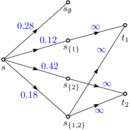
The intuition for the construction and Lemma 3.2 is the following. Each node in corresponds to a possible value vector of all agents, or equivalently, the set of agents whose values are . The flow value from the source to such node is capped by the probability that this value vector is realized. The flow value from a node in to an agent node equals the probability of the event that the vector corresponding to is realized and this agent is selected.
Lemma 3.2.
The set of feasible – maximum flows in corresponds exactly to the set of Full Revelation signaling policies. For any policy , the utility of agent is equal to the total flow to the sink in in the corresponding flow instance.
Proof.
We first prove that any signaling policy can be converted to a maximum flow. Fix any set , and consider the event in which the agents with value exactly form the set . Let be the probability that conditioned on this event, the agent is selected in . We set flow on the edge to be . Note that . The total flow is , which means that it is a maximum flow.
For the other direction, given a maximum flow, let denote the set of agents with value . Notice that when , the flow from to must be equal to its capacity. We construct a Full Revelation signaling policy by requiring that conditioned on being the set of agents with value , the receiver selects with probability , where is the flow on the edge . This is clearly a feasible signaling policy with . ∎
The following theorem (implicit in [Vei71]) shows the existence of a -majorized flow, and therefore shows the existence of a -majorized Full Revelation signaling policy. We include a short proof for completeness.
Theorem 3.3 (-Majorized Flows, Implicit in [Vei71]).
Given any capacitated network with a single source and multiple sinks , let be the flows entering the respective sinks in a feasible flow. Then there is a flow that is -majorized among these feasible flows.
Polynomial-Time Algorithm.
Though the graph constructed above has exponential size, it follows from [Meg74] that a flow is feasible if and only if it is feasible for the following polymatroid :
Maximizing any strictly concave, symmetric, separable function over this polymatroid now yields the solution in polynomial time [Tam95, Vei71]. (See [GM06] for an LP based approach.) This can be solved to an arbitrary approximation in polynomial time.
The final solution for lies in the convex hull of the vertices of . By Carathéodory’s Theorem, this point can be written as the convex combination of at most vertices on the convex hull. By applying an ellipsoid method, we can find such a decomposition in polynomial time. Denote the decomposed vertices and their weights by , where .
By the property of polymatroids, each vertex corresponds to a series of “tight subsets” , where each adjacent pair of sets only differ by a single agent . By a “tight subset” we mean that the inequality is tight at this vertex. Since is the utility of agent for this vertex solution, as long as at least one agent in has value , some agent in this set must be finally selected. This yields the following ranking scheme for :
-
1.
The sender reveals all indices .
-
2.
The receiver selects the first agent in the ranking whose value is .
The signaling scheme corresponding to is a randomization over these ranking schemes: With probability , run the ranking mechanism corresponding to the vertex . Since the utilities of the agents are exactly , this is -majorized. This completes the proof of Theorem 2.5.
3.2 Majorization among Full Information Schemes: Proof of Theorem 2.6
We now show that if we restrict to the space of Full Information mapping policies, there is a selection policy that is -majorized and can be computed in polynomial time. Our technique again reduces to network flow, albeit for a relaxation of the problem. We will use a similar relaxation in Section 4 for the general problem.
We assume that there are possible values in total that support the value distributions . In the remainder of this section, we use the notation to denote these possible values. Let . Let be the event that the largest value is at most . We further define
and
Network Flow Instance.
We will show a network flow instance so that any Full Revelation policy can be relaxed into a feasible flow for this instance. Given , let be the probability that agent has value and is selected conditioned on the event . For the policy , the variables and expected utilities satisfy the following constraints.
| (1) | ||||||
| (2) | ||||||
| (3) |
Conditioned on the event , Eq. 2 says at most one agent with value is selected, and Eq. 3 says the probability that agent has value and is selected is at most , the probability that its value is .
Let , and . We can rewrite the above program as:
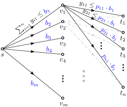
Construct a network flow graph with a source , and one sink for each agent . There are nodes, one for each . There is a directed edge with capacity , and a directed edge with capacity . The flow value on the edge is , and sink receives flow . This shows the network flow instance such that any relaxes to a feasible flow for this instance, and the structure of the network is illustrated in Fig. 2.
Using Theorem 3.3, there is a -majorized flow in , which translates to a -majorized utility vector . Further, this solution can be computed in polynomial time [Tam95, Vei71, GM06]. Denote the majorized solution (in the original variables) as and utilities as .
Signaling Policy.
We now convert the -majorized solution to the above flow instance into a simple -majorized signaling policy. This is inspired by the algorithm for stochastic knapsack [DGV08].
-
•
The sender sends all realized values to the receiver.
-
•
Suppose that the largest realized value is . Let denote the set of agents with value .
-
•
Sort the agents in in a uniformly random order, and consider the agents in this order.
-
•
In this order, when we reach each agent , with probability , select and stop.
-
•
If no agent in is selected above, then select an arbitrary agent in .
Analysis.
Consider any agent . Conditioned on the event (i.e., the largest value being at most ), the probability that another agent is selected before agent is reached is at most
where the factor of comes from the fact that the order is uniformly random. Since , the probability that no agent before is selected is at least . Now, for agent with value to be selected, the following should happen:
-
•
The event , which happens with probability ;
-
•
Agent has value conditioned on , which happens with probability ;
-
•
No agent before is selected conditioned on all previous events, which happens with probability at least ; and
-
•
Agent with value is selected conditioned on all previous events, which happens with probability .
Therefore, the unconditional probability that agent with value is selected is
Therefore, the expected utility of agent in this scheme is at least:
| (4) |
This shows a -majorized signaling scheme running in polynomial time, proving Theorem 2.6.
4 Approximate Majorization: Proof of Theorem 2.8
We now present our main technical result – approximate majorization for general signaling policies. The key hurdle with using the approach in Sections 3.1 and 3.2 is that unlike the Full Revelation setting where the mapping rule is fixed, any mathematical program for general policies needs to encode both mapping and selection variables, and their interaction is non-linear. To deal with the challenge, we will perform a projection of any signaling policy onto a specific class of Single Mean policies, for which the network flow majorization approach in the previous sections can be employed.
4.1 Single Mean Projections
Given a small constant , let . Without loss of generality, assume is a power of , and divide the interval into buckets , where . For any policy , let denote agent ’s utility, that is, . We can express as the sum of contributions from different buckets as , where is the contribution to the utility from those signals for which the posterior mean satisfies .
We now define Single Mean projections that assume that the only contribution to utility for agent happens when the signal received has posterior mean and agent is selected.
Definition 4.1 (Single Mean projection).
Given an interval and signaling policy , let denote the event where both (I) agent is selected and (II) . The Single Mean projection of onto only counts utilities from the event , and sets the remaining utilities to . In other words, if , then for all agents .
Consider now the policy that picks a number uniformly at random and executes the Single Mean projection of for this interval. The expected utility of agent is exactly . We overload the notation and denote the new utilities as .
4.2 Structure of Single Mean Projections
We now show that Single Mean projections can be modified to have a surprisingly simple structure while not decreasing the utilities . Let the interval under consideration be (or if ) and let the Single Mean projection of be . Losing an additional factor in the approximation factor, we can assume that if , then the expected utility of agent is always if is selected.
Note that if and agent is selected, then in this scenario, . Denote the interval as , and as . Assume now that when all agents have posterior mean at most , any agent whose posterior mean is in can be selected, and this choice yields utility to that agent. Such a policy assumes an -approximate utilitarian-welfare-maximizing receiver, and hence our final result will be bicriteria.
Clearly, whenever selects an agent with posterior mean in , all agents must have posterior means at most , so that the new policy can also be made to make the same selection. If we pretend the utility yielded to the agent is , this is still within factor of the actual utility – the modified policy has utilities .
Mathematical Program.
Focus on some , and denote the relaxed Single Mean projection of as . This policy can be written as a distribution over independent signaling schemes as
where each independent signaling scheme is an independent mapping of the agents to signals, along with an associated selection rule, and . For any independent signaling scheme in the above summation, let denote the utility of agent in this scheme, so that
Note that given the Single Mean structure, we only count the utility when the posterior mean of the selected agent lies in , in which case the contribution is assumed to be .
Given signaling scheme , let denote the event that every agent has , where is an independent signal. Now define the following four probabilities for the signaling scheme :
comes from the assumption that in the independent signaling scheme , the mapping rule of each agent is independent of all other agents. The utilities in policy clearly satisfy:
| (5) |
The event conditioned on follows Bernoulli, so that analogous to Section 3.1, the following polymatroid exactly captures the in any feasible policy.
| (6) |
Structural Lemma.
The issue now is that the quantities and depend on the policy , so that we cannot yet reduce it to network flow in a way analogous to Section 3.1. Our key insight is that this dependence can be removed. Towards this end, we define a maximal mapping as follows.
Definition 4.2 (Maximal Mapping).
For an interval , a maximal mapping is a mapping rule from agent values to signals such that is maximized for each agent .
We first show the following structural lemma, and subsequently show how to compute the maximal mapping efficiently.
Lemma 4.3.
Given any independent signaling scheme above, there is an independent signaling scheme that (I) uses a maximal mapping, (II) satisfies Eqs. 5 and 6, and (III) gives each agent a utility of at least from the signals in which their posterior mean is inside , where the contribution to the utility is assumed to be .
Proof.
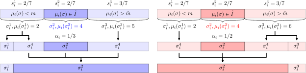
Consider and the corresponding mapping rule for agent . Let be the set of signals with the posterior mean ; be those with ; and those with . Create three signals . These are sent whenever a signal in is sent, respectively. Note that ; ; and . Further, remains unchanged and similarly remains unchanged. This preserves both the constraints and the utilities.
For agent , let satisfy , and define and . Create a new signal , and do the following things:
-
•
If , then whenever signal was sent, is sent instead, and whenever was sent, is sent instead with probability and is sent with probability .
-
•
If , then whenever signal was sent, is sent instead, and whenever was sent, is sent instead with probability and sent with probability .
In either case, we note that . The sender can then send signal whenever is sent, noting that this preserves the condition that .
Note that in either case, does not increase, and hence does not decrease. Since the increase in is exactly the decrease in the sum , we know that does not decrease. Therefore, the solution remains feasible for Eq. 6 with the variables for the new mapping, and the right-hand side in Eq. 5 does not decrease as well, since does not decrease. Therefore, the utility does not decrease. Figure 3 illustrates the reduction process for the two different cases discussed above.
For any agent , the above process yields two signals , where . Recall that is the prior mean, and is a convex combination of and . There are three cases now.
- 1.
- 2.
- 3.
4.3 Reduction to Network Flow and Approximate Majorization
For any agent , the maximal mapping (that maximizes ) is the solution to a linear program. Let denote the probability that the value maps to a signal in , and we have the following linear program.
| maximize: | (7) | |||||
| subject to: | ||||||
Let the optimal objective value of Eq. 7 be . If , then we set and ; if , then we set and ; else we set . Again, let .
We now rewrite the constraints and objective for the independent signaling scheme as follows. Note that and are calculated as above, and do not depend on the policy.
| (8) | ||||||
Note that , and after our transformation above, each now faces the same constraints in Eq. 8. Therefore, we can set , which will be feasible in Eq. 8. In order to reduce to network flow, we will relax the above program to the following:
| (9) | ||||||
Recall from Section 4.1 that we randomize over the projections of the optimal signaling policy , while preserving all utilities to a factor of . For every , consider the relaxed Single Mean policy constructed above. For notational convenience, we denote the in the corresponding maximal mapping as . Further denote the lower end-point of as , and the variable by . Putting together Eq. 9 for different values of , it holds that the utilities of the policy , after losing the factor of , satisfy the following constraints.
| (10) | ||||||
Network Flow and Majorization.
Define and , and we have
| (11) | ||||||
By the same argument as in Section 3.2, the constraints above formulate a network flow problem. The agents are the sinks. Each interval is an intermediate node that is connected to the source with edges of capacity . The node is connected to sink with an edge of capacity . By Theorem 3.3, this network flow problem has a -majorized solution (which is computable in polynomial time according to the discussion in Section 3.1). Consequently, there exist utilities that are -majorized.
Final Algorithm.
Our final algorithm will round the majorized solution analogous to Section 3.2.
-
•
For each , consider the relaxed interval , and compute the quantities using Eq. 7.
-
•
Compute the -majorized solution to Eq. 10.
-
•
Pick a number uniformly at random.
-
•
Given the realized values, compute the corresponding signals via the maximal mapping for and send the signals to the receiver. The receiver selects an agent as follows:
-
–
If any agent has posterior mean larger than the interval , select the agent with the highest mean and stop.
-
–
Consider the agents whose posterior mean lies in in a uniformly random order. For each agent in this order, if it is reached, select it with probability and stop.
-
–
If no agent is selected so far, select the agent with the highest posterior mean.
-
–
Analysis.
The same analysis as Section 3.2 shows that for each agent , the utility in the above algorithm is at least , where is the utility in the -majorized solution to Eq. 10. To see this, note that the probability of selecting the interval is . Conditioned on this event, the probability that no agent has posterior mean larger than is . Conditioned on these two events, the probability that the posterior mean of agent both lies in and is selected is at least , and in this case, it yields utility at least . The overall utility bound now follows by linearity of expectation.
Randomizing over Single Mean projections (see Section 4.1) loses a factor of in each utility, and hence our method gives a bicriteria -majorized solution, completing the proof of Theorem 2.8.
4.4 Extension to Asymmetric Utilities
So far, we have assumed that the receiver’s selection criterion is based on the agents’ signaled values, and the value of the chosen agent is the welfare the system generates. The work of [AK20, DTWZ24] considers a slightly different model, where though the agents signal their values and the receiver selects the agent whose mean posterior signaled value is largest, an individual agent’s utility is if selected and otherwise. This corresponds to the utility perceived by the selfish agent, as opposed to the welfare generated by the system. We observe that the proofs for Theorems 2.8 and 2.6 extends as is to this model, and sketch the changes needed.
To see that the proof of Theorem 2.8 extend as is, we keep the construction of the mathematical program in Section 4.2 the same, except we modify Eq. 5 to
| (12) |
which captures the utility being the same as the probability of being selected. For this modification, the proof of Lemma 4.3 remains unchanged. Subsequently, Eq. 7 remains unchanged, while we change Eq. 10 to
| (13) | ||||||
This again reduces to network flow by defining and , yielding exactly Eq. 11. This completes the proof of Theorem 2.8 for this setting.
Analogously, the proof of Theorem 2.6 extends to this setting by changing the relaxation to replace the value by in the first (utility) constraint Eq. 1. It is easy to check that the resulting program this also reduces to network flow. The rest of the analysis goes through as is, except for replacing by in Eq. 4. This shows a -majorized solution.
5 Lower Bound on Majorization: Proof of Theorem 2.9
We first assume that the receiver is maximizing the utilitarian welfare exactly, and it will become clear that the same lower bound holds if the receiver selects an agent using an arbitrary function of the posterior means – in particular, if it is a -approximate utilitarian welfare maximizer.
Let there be agents. Each agent has value with probability and has value with probability . Note that the expected value of agent is , the same for each . For any , denote by . We first give a lower bound on the sum of the smallest agents’ utilities.
Lemma 5.1.
For any , there exists a signaling policy , such that if the utilities of the agents are arranged in ascending order, the prefix of the first utilities sums to
In order to prove this lemma, we construct the signaling policy as follows. For each agent with , if , then with probability , the sender sends a signal to the receiver, and otherwise the sender sends a signal for this agent. For , the sender reveals the true value of agent . Note that this mapping rule is independent for each agent.
Note that conditioned on receiving signal , we have . On the other hand, conditioned on receiving , we have
Therefore, if at least one signal is received, the receiver will select the agent , with the largest index. On the other hand, if no signal is received, the receiver selects the unique agent with the highest revealed value.
For each , we set
The intuition behind this formula is to have for any . We obtain the utility of all agents as follows.
Lemma 5.2.
It holds that
Proof.
By the construction of , for any , the receiver will receive signal and no signal for with probability
Since agent receives utility if and only if signal is sent and no signal for is sent, we have
Next we consider agent for . By a similar telescoping as above, the probability that no signal with is sent (denoted by ) is
For any agent with , the probability that it has the largest revealed value among agents is
Therefore, the expected utility of agent is
Completing the proof of Lemma 5.1.
We apply the signaling scheme defined above. By Lemma 5.2, we have for all . Thus the agents with smallest expected utilities are agents . Their utilities sum up to
completing the proof. ∎
Proof of Theorem 2.9.
Since , we have
The quantity is a lower bound on the sum of the smallest utilities in the signaling policy . Fix any signaling policy . Suppose that each agent is selected with probability in . If is -majorized, the sum of the utilities of agents in the set must be at least . Therefore, we have the following set of inequalities
We now want to lower bound . The optimal way to assign the probabilities is to make all the inequalities satisfied with equality. Therefore, we have
| (Since ) | ||||
| (Since is monotonically decreasing on [1, n+1]) | ||||
Combining the inequality above with , we have
Since the second part of our argument only requires the fact that at most one agent is selected and is independent of the receiver’s selection rule, this lower bound also applies if the receiver can arbitrarily select the agent, or (in particular) if the receiver is an approximate utilitarian welfare maximizer.
6 Open Directions
Our work points to several interesting future directions. First, we assume independent (or decentralized) mapping of values to signals, motivated hiring and selection applications. Can a similar existence result as in Section 4 extend to the setting where the sender can correlate signals from different agents? We note however that the two settings are somewhat incomparable, and it may very well be that the correlated setting is computationally simpler for a given fairness function [DX16], while the independent case is easier from an approximate majorization perspective.
Secondly, our lower bound in Section 5 holds for distributions with large variance. Is there an -majorized policy under a more benign assumption on distributions, such as the monotone hazard rate (MHR) assumption? Next, we assumed a single agent is finally selected. What if the receiver selects the top agents according to the posterior mean? In this case, it is open if there a polynomial-time algorithm for a given fairness function, in both the cases where the sender can correlate signals and when it sends independent signals. Further, it is an open question to extend our majorization result even to the case when .
Finally, we assume agents are not strategic in revealing information, and our results can be viewed as the limits of fairness that is achievable even if agents follow a prescribed policy. It is an interesting direction to study equilibria and price of anarchy when agents reveal information strategically, building on [AK20, DTWZ24].
References
- [AK20] Pak Hung Au and Keiichi Kawai. Competitive information disclosure by multiple senders. Games and Economic Behavior, 119:56–78, 2020.
- [BBM15] Dirk Bergemann, Benjamin Brooks, and Stephen Morris. The limits of price discrimination. American Economic Review, 105(3):921–957, 2015.
- [BM04] Marianne Bertrand and Sendhil Mullainathan. Are Emily and Greg more employable than Lakisha and Jamal? A field experiment on labor market discrimination. American Economic Review, 94(4):991–1013, 2004.
- [BM19] Dirk Bergemann and Stephen Morris. Information design: A unified perspective. Journal of Economic Literature, 57(1):44–95, 2019.
- [BMSW24] Siddhartha Banerjee, Kamesh Munagala, Yiheng Shen, and Kangning Wang. Fair price discrimination. In Proceedings of the 2024 ACM-SIAM Symposium on Discrete Algorithms (SODA), pages 2679–2703. SIAM, 2024.
- [BTXZ21] Yakov Babichenko, Inbal Talgam-Cohen, Haifeng Xu, and Konstantin Zabarnyi. Regret-minimizing bayesian persuasion. In Proceedings of the 22nd ACM Conference on Economics and Computation (EC), page 128. ACM, 2021.
- [CDHW20] Rachel Cummings, Nikhil R. Devanur, Zhiyi Huang, and Xiangning Wang. Algorithmic price discrimination. In Proceedings of the 2020 ACM-SIAM Symposium on Discrete Algorithms (SODA), pages 2432–2451. SIAM, 2020.
- [CDW12] Yang Cai, Constantinos Daskalakis, and S. Matthew Weinberg. Optimal multi-dimensional mechanism design: Reducing revenue to welfare maximization. In Proceedings of the 53rd Annual IEEE Symposium on Foundations of Computer Science (FOCS), pages 130–139. IEEE Computer Society, 2012.
- [CH14] Archishman Chakraborty and Rick Harbaugh. Persuasive puffery. Marketing Science, 33(3):382–400, 2014.
- [CMV20] L. Elisa Celis, Anay Mehrotra, and Nisheeth K. Vishnoi. Interventions for ranking in the presence of implicit bias. In Proceedings of the 2020 ACM Conference on Fairness, Accountability, and Transparency (FAT*), pages 369–380. ACM, 2020.
- [CS19] Deeparnab Chakrabarty and Chaitanya Swamy. Approximation algorithms for minimum norm and ordered optimization problems. In Proceedings of the 51st Annual ACM SIGACT Symposium on Theory of Computing (STOC), pages 126–137. ACM, 2019.
- [DGV08] Brian C. Dean, Michel X. Goemans, and Jan Vondrák. Approximating the stochastic knapsack problem: The benefit of adaptivity. Mathematics of Operations Research, 33(4):945–964, 2008.
- [DKKS24] Siddartha Devic, Aleksandra Korolova, David Kempe, and Vatsal Sharan. Stability and multigroup fairness in ranking with uncertain predictions. In Proceedings of the 41st International Conference on Machine Learning (ICML). PMLR, 2024.
- [DKQ16] Shaddin Dughmi, David Kempe, and Ruixin Qiang. Persuasion with limited communication. In Proceedings of the 17th ACM Conference on Economics and Computation (EC), pages 663–680. ACM, 2016.
- [DR89] Bhaskar Dutta and Debraj Ray. A concept of egalitarianism under participation constraints. Econometrica, 57(3):615–635, 1989.
- [DREM13] Ezekiel J. Dixon-Román, Howard T. Everson, and John J. McArdle. Race, poverty and SAT scores: Modeling the influences of family income on black and white high school students’ SAT performance. Teachers College Record, 115(4):1–33, 2013.
- [DTWZ24] Zhicheng Du, Wei Tang, Zihe Wang, and Shuo Zhang. Competitive information design with asymmetric senders. In Proceedings of the 25th ACM Conference on Economics and Computation (EC)), 2024.
- [Dug17] Shaddin Dughmi. Algorithmic information structure design: a survey. SIGecom Exchanges, 15(2):2–24, 2017.
- [DX16] Shaddin Dughmi and Haifeng Xu. Algorithmic bayesian persuasion. In Daniel Wichs and Yishay Mansour, editors, Proceedings of the 48th Annual ACM SIGACT Symposium on Theory of Computing (STOC), pages 412–425. ACM, 2016.
- [EGGL20] Vitalii Emelianov, Nicolas Gast, Krishna P. Gummadi, and Patrick Loiseau. On fair selection in the presence of implicit variance. In Proceedings of the 21st ACM Conference on Economics and Computation (EC), pages 649–675. ACM, 2020.
- [GB21] David García-Soriano and Francesco Bonchi. Maxmin-fair ranking: Individual fairness under group-fairness constraints. In Proceedings of 27th ACM SIGKDD Conference on Knowledge Discovery and Data Mining (KDD), pages 436–446. ACM, 2021.
- [GM06] Ashish Goel and Adam Meyerson. Simultaneous optimization via approximate majorization for concave profits or convex costs. Algorithmica, 44(4):301–323, 2006.
- [GMP05] Ashish Goel, Adam Meyerson, and Serge A. Plotkin. Approximate majorization and fair online load balancing. ACM Transactions on Algorithms, 1(2):338–349, 2005.
- [GMS10] Sudipto Guha, Kamesh Munagala, and Peng Shi. Approximation algorithms for restless bandit problems. Journal of the ACM, 58(1):3:1–3:50, 2010.
- [GR00] Claudia Goldin and Cecilia Rouse. Orchestrating impartiality: The impact of “blind” auditions on female musicians. American Economic Review, 90(4):715–741, 2000.
- [HLP34] Godfrey Harold Hardy, John Edensor Littlewood, and George Pólya. Inequalities. Cambridge university press, 1934.
- [Kar32] Jovan Karamata. Sur une inégalité relative aux fonctions convexes. Publications de l’Institut Mathematique, 1(1):145–147, 1932.
- [KG11] Emir Kamenica and Matthew Gentzkow. Bayesian persuasion. American Economic Review, 101(6):2590–2615, 2011.
- [KK06] Amit Kumar and Jon M. Kleinberg. Fairness measures for resource allocation. SIAM Journal on Computing, 36(3):657–680, 2006.
- [KR18] Jon M. Kleinberg and Manish Raghavan. Selection problems in the presence of implicit bias. In Proceedings of the 9th Conference on Innovations in Theoretical Computer Science Conference (ITCS), pages 33:1–33:17. Schloss Dagstuhl - Leibniz-Zentrum für Informatik, 2018.
- [MC21] Anay Mehrotra and L. Elisa Celis. Mitigating bias in set selection with noisy protected attributes. In Proceedings of the 2021 ACM Conference on Fairness, Accountability, and Transparency (FAccT), pages 237–248. ACM, 2021.
- [Meg74] Nimrod Megiddo. Optimal flows in networks with multiple sources and sinks. Mathematical Programming, 7:97–107, 1974.
- [SKJ21] Ashudeep Singh, David Kempe, and Thorsten Joachims. Fairness in ranking under uncertainty. In Proceedings of the 35th Annual Conference on Neural Information Processing Systems (NeurIPS), pages 11896–11908, 2021.
- [SWZ+23] Zeyu Shen, Zhiyi Wang, Xingyu Zhu, Brandon Fain, and Kamesh Munagala. Fairness in the assignment problem with uncertain priorities. In Proceedings of the 2023 International Conference on Autonomous Agents and Multiagent Systems (AAMAS), pages 188–196. ACM, 2023.
- [Tam95] Arie Tamir. Least majorized elements and generalized polymatroids. Mathematics of Operations Research, 20(3):583–589, 1995.
- [Vei71] Arthur F. Veinott Jr. Least -majorized network flows with inventory and statistical applications. Management Science, 17(9):547–567, 1971.
- [XRDT15] Haifeng Xu, Zinovi Rabinovich, Shaddin Dughmi, and Milind Tambe. Exploring information asymmetry in two-stage security games. In Proceedings of the 29th AAAI Conference on Artificial Intelligence (AAAI), pages 1057–1063. AAAI Press, 2015.