Theory of vibronic adsorbate-surface Fano resonances
Abstract
Inspired by recent visible pump - infrared probe spectra reported for molecular catalysts adsorbed to quantum dots, we introduce a theory of non-equilibrium vibronic Fano resonances arising from the interference of quantum dot excited-state intraband transitions and infrared vibrational excitations of a molecular adsorbate. Our theory suggests a superexchange mechanism for the observed Fano resonances where charge-transfer states mediate the effective interaction between molecular vibrations and near-resonance quantum dot intraband transitions. We present a perturbative treatment of the effective adsorbate-quantum dot vibronic interaction and employ it to construct a two-reservoir Fano model that enables us to capture key experimental trends, including the relationship between the Fano asymmetry factor, quantum dot size, and the distance between the molecular adsorbate and the quantum dot. We focus on adsorbate-quantum dot species, but our theory’s implications are shown to be generic for molecules adsorbed to materials with resonant strong mid-infrared electronic transitions.
I Introduction
Fano resonances emerge from the hybridization of interacting discrete and continuum states of a system [1] and have been observed in the autoionization spectra of atoms [2, 3], carbon nanotube transport [4, 5], doped-Si Raman scattering [6], scanning tunneling microscopy (STM) measurements of mesoscopic systems with impurities [7, 8, 9, 10], and plasmonic materials [11, 12]. Basic interest in Fano resonances stems from their role in fundamental processes underlying energy relaxation and conversion[13, 14] and charge transport in materials [15, 16]. Applications also abound in metamaterials and nanophotonics [17, 18, 19, 20, 21, 22], where the high sensitivity of Fano resonances to geometric and environmental changes is promising for a range of applications including sensing [23, 24, 25, 26], near-field imaging [27, 28, 29], and nonlinear optics [30, 31].
Recently, Yang et al. [32] and Gebre et al. [33, 34] reported the observation of Fano-like asymmetric lineshapes in the pump-probe spectrum of inorganic transition metal complexes adsorbed to CdS and CdSe nanocrystals. In these experiments, a visible pump photon generates a QD exciton corresponding to a nanocrystal state with broad infrared adsorption that overlaps with molecular vibrational transitions of the adsorbed molecules. This feature gives rise to the reported Fano resonances observed in the ultrafast infrared probe spectrum, which arise from the interference of the molecular normal-mode transition and the intraband excitation of the photogenerated electron.
In Ref. [33], the measured Fano asymmetry factors observed for QD-adsorbate complexes show characteristic dependence on the QD size. Similarly, Ref. [34] reports the variation of the Fano asymmetry with the distance between the QD and the adsorbate. These variations positively correlate with charge-transfer rates and suggest tunable vibronic interactions between the QD and the molecular adsorbate. In this article, we propose an effective theoretical model and microscopic mechanism for Fano resonances arising from the interference of quantum dot intraband transitions and vibrational excitations of adsorbed molecules. Our theory is validated by comparing its predictions for the size and distance-dependence of experimentally obtained Fano asymmetry factors in recent experiments [33, 34]. In Sec. II, we introduce our theoretical model and describe its underlying assumptions. Sec. III provides a derivation of the effective interaction between the molecular vibrations and the QD intraband transitions and the associated vibronic Fano resonance lineshape and discusses its predictions in the context of recent experiments. Sec. IV summarizes our main results and conclusions.
II Theory
We model the quantum dot and its interaction with the molecular system via a tight-binding model. The QD is represented by its 1S and 1P electronic states and bath modes, whereas the molecular electronic Hilbert space is characterized by the occupation of the lowest unoccupied molecular orbital (LUMO). Vibronic coupling in the molecular subsystem is treated using the displaced oscillator model, indicating the ionic molecular species has a different equilibrium geometry than the neutral state. The interaction between the molecular system and the QD is represented by transition matrix elements enabling electron hopping from the QD into the LUMO and vice-versa. In the following subsections, we describe in detail the molecular, quantum dot, and interaction Hamiltonians employed to derive a vibronic IR Fano lineshape for molecules adsorbed to QDs.
II.1 Molecular, quantum dot and interaction Hamiltonians
The total Hilbert space of our system is a direct product of the quantum dot Hilbert space and the molecular vibrational-electronic space of states. The quantum dot electronic states correspond to the lowest energy exciton state, 1S, and the 1P exciton state accessible by IR excitation. The 1S 1P absorption is extremely broad due to the coupling of the 1P exciton with bath degrees of freedom (e.g., quantum dot phonons). The molecular electronic states are characterized by the occupation of the LUMO, and the vibrational degrees of freedom are represented by a single mode assumed to be harmonic for simplicity. Therefore, the quantum states in our system can be classified into neutral () or ionic (), wherein the neutral manifold, the LUMO state has vanishing occupation number, and the QD is in the 1S or 1P state. The ionic states consist of all levels where an electron occupies the LUMO, and the QD has a single hole in its valence band.
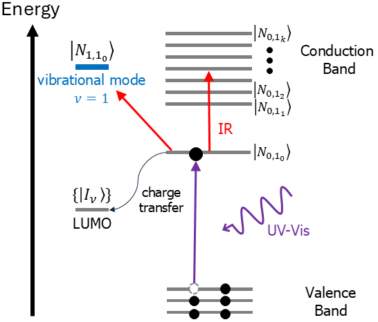
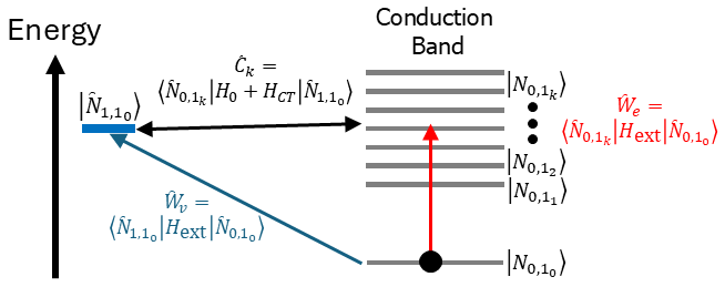
We denote the neutral states by corresponding to the quantum dot in electronic state ( if the QD occupies electronic level corresponding to 1P and bath state represented by , and if the QD is in the 1S state), and the molecule is in its electronic ground-state at vibrational level . The initial state (experimentally obtained after pumping the QD using a visible pulse) (Fig. 1) in our analysis is therefore . The set of ionic states is denoted by , where labels the molecular vibrational quantum number and the QD is electron deficient. In Fig. 1, we provide a schematic representation of our model.
Our model has Hamiltonian given by
| (1) |
where is the molecular part, is the QD Hamiltonian, includes the charge-transfer interaction of the QD with the adsorbate and is the interaction of the system with an external radiation field. It is useful to partition the Hamiltonian into , where is the noninteracting Hamiltonian describing the isolated QD and molecule, and contains the charge-transfer interaction and the coupling to the external field.
The molecular system is assumed to have distinct equilibrium geometries in the neutral (vanishing LUMO occupation) and ionic states. Therefore, is given by
| (2) |
where is the vibrational quantum number of the molecular system, is equal to the sum of the electronic energy of the adsorbate and quantum dot, is the molecular vibrational frequency, denotes vibrational quantum number in the ionic state, and is the electronic-vibrational energy of the corresponding ionic state.
In what follows, for the sake of simplicity, we will only explicitly consider dynamics involving neutral states and and their coupling to generic ionic states. These two states are relevant because they correspond to the dominant contributions to the initial and final states of the infrared absorption process of interest.
The interaction Hamiltonian contains the electronic coupling promoting charge transfer between the QD and molecular species [35, 36, 37] and is given by
| (3) |
where and are vibronic hopping amplitudes between the QD and the molecular LUMO (ionic state) accompanied by a transition into the vibrational state [38, 39], i.e., the electron hopping element indicates an electron transfer from the neutral to ionic state and a transition of the vibrational molecular states of the form . A detailed description of how the electronic hopping amplitudes are estimated as a function of the various relevant parameters characterizing the QD is given in the next subsection.
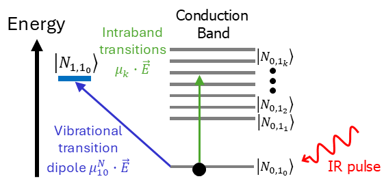
The interaction with the external field models the IR probe pulse induced electronic intraband transition of the QD [40] and vibrational transitions of the molecular system in the neutral and ionic states [41, 42, 43]
| (4) |
Here, represents the IR electric field, and () denotes the vibrational transition dipole matrix element between the vibrational states () when the molecular-QD system is in the neutral (ionic) state, whereas is the QD electronic intraband transition dipole moment for the lowest energy exciton state into the state. In Figure (2), we show a schematic representation of the electronic and vibrational transitions induced by the external field (IR probe pulse).
II.2 Electronic coupling
The electronic coupling between the QD surface and the adsorbed molecule, denoted by , is determined by the electronic interaction between both species
| (5) |
where is the electronic wavefunction of the LUMO, is a QD state, and is the (mean-field) electronic interaction Hamiltonian. For the sake of simplicity, since our analysis below is focused on investigating variations of the QD-adsorbate effective interaction with QD properties independent of molecular vibrational degrees of freedom, we ignore the vibrational part of the adsorbate and QD wave function in this section.
The penetration amplitude of the molecular wavefunction into the QD bulk is negligible and, therefore, neglected. In this case, the electronic overlap is only significant near the surface [44], and the electronic hopping integral can be written as
| (6) |
where is the QD radius. Assuming a perfectly spherical QD and using Eq. (24), we find
| (7) |
This implies the electronic hopping parameter is approximately proportional to . Given that decays exponentially and thus much faster than increases with the QD size, the charge transfer amplitude is anticipated to become less efficient with increasing QD size.
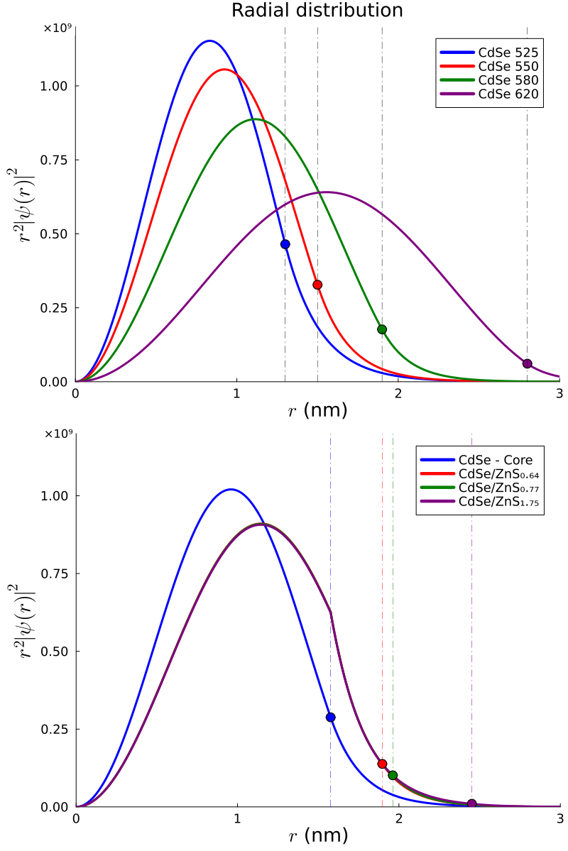
In the experiments discussed in Ref. [34], core/shell QDs were employed to modulate the interaction between the QD and the molecular adsorbate. Specifically, the shell thickness enabled control of the overlap between the adsorbate and the QD exciton wave functions. Appendix A describes our procedure for estimating the exciton wave function in core/shell QD structures. In Fig. 3, we show the obtained radial distribution of 1S electronic wave functions of the core QD at various radii and for core/shell structures at different shell thicknesses.
III Results and Discussion
In this section, we employ the Hamiltonian described in the previous section and perturbation theory to describe the emergence of an effective interaction between QD intraband transitions and adsorbate vibrations via virtual charge transfer processes. This interaction is then applied in a two-reservoir Fano model to characterize the behavior of previously reported variation with QD size and molecular distance of IR Fano lineshapes.
III.1 Vibronic Fano resonances
In our vibronic model, the relevant part of the Hilbert space for analysis of the IR adsorbate-QD Fano resonances in Refs. [33] and [34] is spanned by the 0th-order molecular vibrational state (the discrete final state), the electronic states of the quantum dot (QD) embedded in the continuum , the lowest energy electronic state in the vibrational ground-state , and the set of ionic states (ReC0A- QD+) with variable vibrational quantum number . The ionic states weakly mix with the neutral via the charge-transfer interaction and inspired by first-order perturbation theory, we define a new basis for neutral and ionic species where the relevant states in what follows are given by
| (8) | ||||
| (9) | ||||
| (10) |
and the parameters are normalization coefficients. Using these new states (and their orthogonal complement), we obtain a unitarily transformed Hamiltonian with effective interactions between the near-resonance vibrational excitation and the excited QD states (see Appendix B for further details) suggesting hybridization between discrete and continuum levels with eigenstates
| (11) |
connected to the initial-state via the external radiation field and . It follows the probability of excitation between the initial state and the stationary leads to the Fano lineshape
| (12) |
where is the reduced IR photon energy, is the Fano asymmetry parameter, and denotes the number of levels of the discretized continuum within the natural width. The Fano asymmetry parameter is given by”
| (13) | ||||
| (14) |
where is the vibrational transition dipole moment matrix element, is the effective coupling between the molecular vibrations and the continuum QD electronic states, and is the 1S 1P electronic transition dipole moment. The parameters and model the interaction of the relevant adsorbate vibrational mode with other degrees of freedom that lead to homogeneous broadening of the molecular vibrational excitation and its characteristic Lorenzian lineshape which is present even when the QD is in its ground-state (prior to UV excitation in the experiments of Ref. [33] and [34]). In the presence of the effective coupling to the QD transition, the vibrational dephasing rate is therefore estimated by
| (15) |
where is the average density of states of the two reservoirs. The effective coupling of the second reservoir is expected to be greater since the experiments of Refs. [33] and [34] show the molecular vibrational lineshape is barely affected by the coupling to the excited QD, and in fact, the dominant effect of the latter is in renormalizing the infrared oscillator strength of the vibrational transition. Thus, the effective coupling with the intramolecular or solvent degrees of freedom is expected to be much greater than the QD electronic intraband transitions and . Figure 7 shows a schematic representation of the Fano parameters and the states involved in the vibronic Fano resonance.
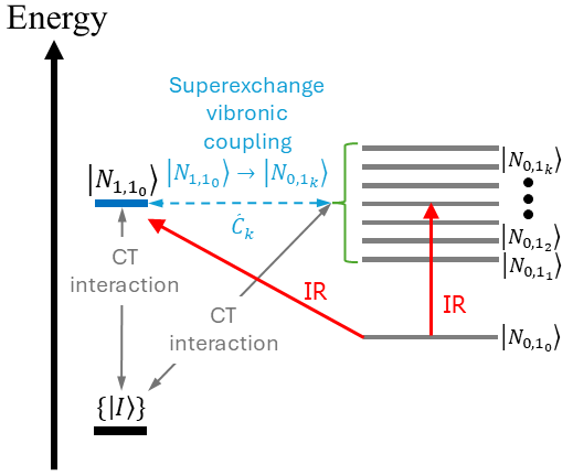
We present in Appendix B detailed explicit derivations of all parameters in Eq. (13). Here, we highlight the effective interaction of the discrete state (molecular vibrations) with the electronic QD continuum states (IR intraband transitions) and denoted by are due to a superexchange process mediated by the CT interaction
| (16) |
This interaction is schematically illustrated in Fig. 4.
We utilize the expressions in Eqs. (31)-(32) and Eq. (16) to derive the Fano asymmetry lineshapes described by Equation (13). To simplify the Fano parameters, we employ the following approximations highlighting their dependence on the electronic coupling strength, denoted by .
First, we address the light-induced interaction of the initial state with the molecular vibration as
| (17) |
where captures the contributions of the vibrational transition dipole moment induced by the weak admixture with the ionic state:
| (18) |
Second, in the regime of small electronic hopping, the intraband transitions involving the lowest QD exciton state and the continuum states () are primarily governed by . Consequently, we assume is independent of the CT process, simplifying it to (interaction from the initial state to the QD 1P states in the unperturbed basis).
Lastly, we approximate the summation over all intermediate ionic states contributing to by a constant. This simplification highlights the dominant dependence of on the electronic coupling strength, . Consequently, in the Fano asymmetry factor in Eq. (14), we replace by with a dimensionless quantity.
Substituting these approximations into the Fano asymmetry factor given by Eq. (14) we obtain
| (19) |
where we introduced the notation (). In Eq. (19), quantifies the vibrational dephasing into the molecular reservoir present even when the QD is in its ground-state, and here we have also assumed that the average density of states is independent of energy and remains constant across various QD sizes. This assumption is consistent with our approximation that the continuum density of states represents the average of the molecular and QD and is independent of the QD size or the molecular distance to the QD.
Eq. 19 is one of the main results of this work. It expresses the Fano asymmetry factor in terms of the molecular-QD electron hopping amplitude . This quantity plays a key role in setting the Fano asymmetry factor because it (1) renormalizes the vibrational oscillator strength, substantially enhancing the infrared absorption strength relative to the unperturbed neutral state, and (2) it also controls how much vibrational energy is dumped into the QD in comparison to the molecular reservoir. Below, we discuss the implications of our formalism.
III.2 Size and distance dependence of Fano resonance
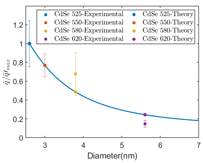
In this subsection, we connect our theoretical findings on the Fano asymmetry factor (Eq. 19) with experimental data by exploring its dependence on the QD size and shell thickness. The molecular parameters and were assumed independent of system size and adjusted by fitting them to experimental data using a distance minimization algorithm. Our analysis focuses on how the electronic coupling between the LUMO of the molecular adsorbate and the QD influences the Fano resonance, with particular attention to the contributions of vibrational transition dipoles and decay rates for CdSe and CdSe/ZnS quantum dots.
Figure 5a reveals agreement between our theoretical predictions and experimental observations regarding the variation of with QD size, where the factor decreases as the QD size increases. The size-dependent behavior of is primarily governed by the electronic coupling between the exciton state and the molecular LUMO, which is modulated by the QD size. A closer to symmetric absorption () indicates an enhanced electronic coupling between the QD exciton and ionic electronic molecular states. Notably, the vibrational transition dipole in the ionic state of the molecular-QD system plays a dominant role in determining (second term in Eq. 17), highlighting the complex interplay between electronic and vibrational dynamics in these nanoscale systems. Finally, the molecular dephasing, in principle, induced by interaction with the QD electronic transition and other degrees of freedom, is predominantly governed by the molecular mechanism consistent with the approximations in Eq. 15.
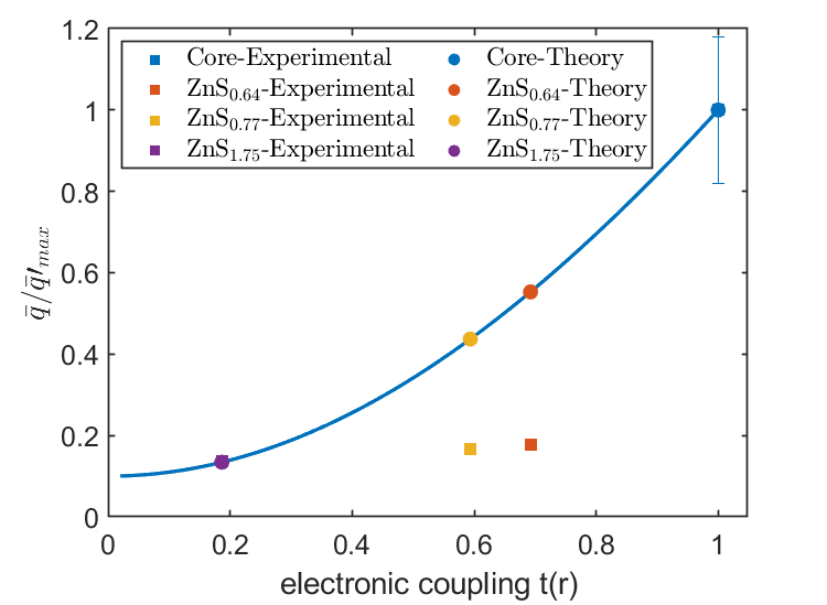
In Fig. 6, we show the behavior of the Fano asymmetry parameter in core/shell QDs with variable thickness. The figure indicates a clear decrease in the normalized Fano asymmetry factor with increasing shell thickness (0, 1, 3, and 6 monolayers) in CdSe/ZnS core/shell QDs, in reasonable agreement with experimental findings. The observed error margin between experimental and theoretical Fano asymmetry parameter dependence on adsorbate-QD distance is largely due to the challenges in modeling the 1S excitonic wavefunction in core/shell QDs and may also be due to potential variation of bare ionic and neutral molecular vibrational transition dipole moments with the core/shell structure. Despite these approximations, the observed trend indicates a weakening of the QD-adsorbed molecule electronic coupling as the shell thickness increases (Fig. 6b) in agreement with the behavior observed with charge-transfer rates [34].
IV Conclusions
This work introduced a superexchange mechanism for vibronic Fano resonances observed in visible pump-IR probe measurements of molecules adsorbed to QDs. Our proposed mechanism involves coupling the molecular CO vibration with the electronic conduction states of the QD through virtual charge-transfer interactions mediated by vibronic coupling with the LUMO. By incorporating the vibronic coupling of the exciton state with the LUMO of the molecular adsorbate, we obtained an approximate expression for the Fano asymmetry parameter in terms of the charge-transfer coupling (Eq. (19)). This model successfully captures several experimental observations across various QD configurations, including the reported decrease in the Fano asymmetry factor with increasing QD size and distance to the adsorbate—reflecting the reduced electronic coupling between the QD exciton and the vibrational molecular states.
The microscopic mechanism provided for vibronic Fano resonances in this work applies broadly and is expected to be observable in visible pump-IR probe measurements whenever molecular vibrations are near-resonant with infrared electronic transitions of QDs or other nanoparticles. Future experiments and ab initio quantum chemistry simulations provide promising avenues for unraveling further details of the Fano resonances discussed in this work, including the role of the solvent interactions with the QD and the molecular adsorbate.
Acknowledgments. This material is based upon work supported by the U.S. Department of Energy, Office of Science, Office of Basic Energy Sciences, Solar Photochemistry Program under Award Number DE-SC0008798. R.F.R acknowledges support from NSF CAREER award Grant No. CHE-2340746 and startup funds provided by Emory University. S.T.G acknowledges support from AGEP supplement to NSF award number CHE-2004080.
Appendix A Quantum dot wave functions
The Schrodinger equation for the electron-hole quantum dot wave function and its corresponding energies can be written in spherical coordinates as:
| (20) |
where is the electron effective mass in the conduction band in the -th layer on the QD, and we have assumed a radial dependence on the potential energy . Note that the conduction band edge energy determines the potential energy [45]. Thus, we define the potential energy for the bare QD with radius as:
| (21) |
with effective mass . In the Core/Shell structure with inner radius and total radius , we define the potential energy as
| (22) |
and effective mass
| (23) |
Since we have assumed a perfect spherical QD, and given the potentials (21)-(22), we can split the wavefunction into its radial and angular (spherical harmonics function) parts:
| (24) |
where is the polar and is the azimuthal angle. The detailed solutions of Eq. (A) can be found in [44] with the following boundary conditions in the interface between the Core/Shell:
| (25) | ||||
| (26) |
The QD size and solvent have been shown to influence the edge band energy. For instance, [45] proposed an empirical formula to calculate the conduction band edge energy for CdSe QD given by:
| (27) |
is the QD diameter, and is the bulk conduction band edge energy relative to a solvent with dielectric constant . The conduction band edge position of the complex ZnS relative to the CdSe in a core/shell QD ranges from to . The values reported here () are chosen to emphasize the shell thickness dependence on the Fano asymmetry factor.
Appendix B Quantum Fano resonance parameters from perturbation theory
The Fano parameters of (13) are described by the set of perturbed eigenstates (8)-(10) interacting via vibronic coupling with the LUMO. Thus, the Fano parameters are defined as follows:
| (28) | ||||
| (29) | ||||
| (30) |
The Fano parameters (28)-(30) can be written by replacing the perturbed eigenstates (31)-(16) and ignoring higher orders of on the electron hopping as:
| (31) | ||||
| (32) |
Equations (32)-(16) delineate the Fano lineshape parameter, highlighting its dependence on the electronic hopping terms and . Fig. 7 illustrates the Fano parameters and their states involved in the interaction. Note that the Fano parameters described in Eq. (13) corresponds to the perturbed eigenstates induced by vibronic coupling.
In Eq. (16) we have established the coupling between molecular vibrations and the discrete states of the QD, denoted by , through the electronic coupling mediated by the virtual molecular ionic state (LUMO). This interaction occurs through the following: 1) the molecular vibrational modes in the neutral species interact with the virtual Ionic states through the vibronic coupling , 2) the Ionic species weakly mixes with the QD electronic conduction band , and 3) the discrete molecular phonon mode interacts with the electronic continuum via the CT mediated by the virtual vibrational ionic intermediate state in a superexchange process . Thus, the Fano asymmetry factor q depends on the electronic coupling between the catalyst and the electronic QD states. To illustrate the superexchange mechanism, Figure 4 presents a schematic representation. Here, we show the interaction between the discrete vibrational state and the electronic continuum of the QD.
To facilitate the understanding of the fitting parameters for the Fano asymmetry factor in Eq. (19), we will label the following parameters as and , such that is clear in Eq. (19) the contributions of the Ionic species, and the QD electronic states:
| (34) |
To minimize the number of parameters in our model (34), we normalize the Fano asymmetry factor by the QD with maximum , i.e., by its maximum value at
| (35) |
Here, is associated with the ratio of the vibrational transition matrix element in the adsorbate ionic state relative to the same quantity for the neutral species of the QD-adsorbate system with electron hopping amplitude and representing the ratio of transition dipole moments for the 1S 1P transition to the vibrational transition matrix element at the resonance frequency of the latter.
References
- Fano [1961] U. Fano, Effects of configuration interaction on intensities and phase shifts, Physical review 124, 1866 (1961).
- Rice [1933] O. Rice, Predissociation and the crossing of molecular potential energy curves, The Journal of Chemical Physics 1, 375 (1933).
- Beutler [1935] H. Beutler, Über absorptionsserien von argon, krypton und xenon zu termen zwischen den beiden ionisierungsgrenzen 2 p 3 2/0 und 2 p 1 2/0, Zeitschrift für Physik 93, 177 (1935).
- Del Valle et al. [2005] M. Del Valle, C. Tejedor, and G. Cuniberti, Defective transport properties of three-terminal carbon nanotube junctions, Physical Review B 71, 125306 (2005).
- Kim et al. [2003] J. Kim, J.-R. Kim, J.-O. Lee, J. W. Park, H. M. So, N. Kim, K. Kang, K.-H. Yoo, and J.-J. Kim, Fano resonance in crossed carbon nanotubes, Physical review letters 90, 166403 (2003).
- Cerdeira et al. [1973] F. Cerdeira, T. Fjeldly, and M. Cardona, Effect of free carriers on zone-center vibrational modes in heavily doped p-type si. ii. optical modes, Physical Review B 8, 4734 (1973).
- Li et al. [1998] J. Li, W.-D. Schneider, R. Berndt, and B. Delley, Kondo scattering observed at a single magnetic impurity, Physical Review Letters 80, 2893 (1998).
- Madhavan et al. [1998] V. Madhavan, W. Chen, T. Jamneala, M. Crommie, and N. Wingreen, Tunneling into a single magnetic atom: spectroscopic evidence of the kondo resonance, Science 280, 567 (1998).
- Luo et al. [2004] H. Luo, T. Xiang, X. Wang, Z. Su, and L. Yu, Fano resonance for anderson impurity systems, Physical review letters 92, 256602 (2004).
- Újsághy et al. [2000] O. Újsághy, J. Kroha, L. Szunyogh, and A. Zawadowski, Theory of the fano resonance in the stm tunneling density of states due to a single kondo impurity, Physical review letters 85, 2557 (2000).
- Luk’Yanchuk et al. [2010] B. Luk’Yanchuk, N. I. Zheludev, S. A. Maier, N. J. Halas, P. Nordlander, H. Giessen, and C. T. Chong, The fano resonance in plasmonic nanostructures and metamaterials, Nature materials 9, 707 (2010).
- Liu et al. [2017a] Z. Liu, J. Li, Z. Liu, W. Li, J. Li, C. Gu, and Z.-Y. Li, Fano resonance rabi splitting of surface plasmons, Scientific reports 7, 8010 (2017a).
- Liu et al. [2017b] B. Liu, C. Tang, J. Chen, M. Zhu, M. Pei, and X. Zhu, Electrically tunable fano resonance from the coupling between interband transition in monolayer graphene and magnetic dipole in metamaterials, Scientific Reports 7, 17117 (2017b).
- Giannini et al. [2011] V. Giannini, Y. Francescato, H. Amrania, C. C. Phillips, and S. A. Maier, Fano resonances in nanoscale plasmonic systems: a parameter-free modeling approach, Nano letters 11, 2835 (2011).
- Miroshnichenko et al. [2010] A. E. Miroshnichenko, S. Flach, and Y. S. Kivshar, Fano resonances in nanoscale structures, Reviews of Modern Physics 82, 2257 (2010).
- Xiao et al. [2016] S. Xiao, Y. Yoon, Y.-H. Lee, J. Bird, Y. Ochiai, N. Aoki, J. Reno, and J. Fransson, Detecting weak coupling in mesoscopic systems with a nonequilibrium fano resonance, Physical Review B 93, 165435 (2016).
- Song et al. [2006] J. Song, R. P. Zaccaria, M. Yu, and X. Sun, Tunable fano resonance in photonic crystal slabs, Optics express 14, 8812 (2006).
- Yu et al. [2014] Y. Yu, M. Heuck, H. Hu, W. Xue, C. Peucheret, Y. Chen, L. K. Oxenløwe, K. Yvind, and J. Mørk, Fano resonance control in a photonic crystal structure and its application to ultrafast switching, Applied physics letters 105 (2014).
- Zhou et al. [2014] W. Zhou, D. Zhao, Y.-C. Shuai, H. Yang, S. Chuwongin, A. Chadha, J.-H. Seo, K. X. Wang, V. Liu, Z. Ma, et al., Progress in 2d photonic crystal fano resonance photonics, Progress in Quantum Electronics 38, 1 (2014).
- Limonov et al. [2017] M. F. Limonov, M. V. Rybin, A. N. Poddubny, and Y. S. Kivshar, Fano resonances in photonics, Nature photonics 11, 543 (2017).
- Gao et al. [2018] W. Gao, X. Hu, C. Li, J. Yang, Z. Chai, J. Xie, and Q. Gong, Fano-resonance in one-dimensional topological photonic crystal heterostructure, Optics express 26, 8634 (2018).
- Bekele et al. [2019] D. Bekele, Y. Yu, K. Yvind, and J. Mork, In-plane photonic crystal devices using fano resonances, Laser & Photonics Reviews 13, 1900054 (2019).
- Hao et al. [2008] F. Hao, Y. Sonnefraud, P. V. Dorpe, S. A. Maier, N. J. Halas, and P. Nordlander, Symmetry breaking in plasmonic nanocavities: subradiant lspr sensing and a tunable fano resonance, Nano letters 8, 3983 (2008).
- Chen et al. [2018] J. Chen, F. Gan, Y. Wang, and G. Li, Plasmonic sensing and modulation based on fano resonances, Advanced Optical Materials 6, 1701152 (2018).
- Wu et al. [2012] C. Wu, A. B. Khanikaev, R. Adato, N. Arju, A. A. Yanik, H. Altug, and G. Shvets, Fano-resonant asymmetric metamaterials for ultrasensitive spectroscopy and identification of molecular monolayers, Nature materials 11, 69 (2012).
- King et al. [2015] N. S. King, L. Liu, X. Yang, B. Cerjan, H. O. Everitt, P. Nordlander, and N. J. Halas, Fano resonant aluminum nanoclusters for plasmonic colorimetric sensing, ACS nano 9, 10628 (2015).
- Luk’Yanchuk et al. [2013] B. Luk’Yanchuk, A. Miroshnichenko, and Y. S. Kivshar, Fano resonances and topological optics: an interplay of far-and near-field interference phenomena, Journal of Optics 15, 073001 (2013).
- Song et al. [2016] M. Song, C. Wang, Z. Zhao, M. Pu, L. Liu, W. Zhang, H. Yu, and X. Luo, Nanofocusing beyond the near-field diffraction limit via plasmonic fano resonance, Nanoscale 8, 1635 (2016).
- Conteduca et al. [2023] D. Conteduca, S. N. Khan, M. A. Martinez Ruiz, G. D. Bruce, T. F. Krauss, and K. Dholakia, Fano resonance-assisted all-dielectric array for enhanced near-field optical trapping of nanoparticles, ACS photonics 10, 4322 (2023).
- Piao et al. [2015] X. Piao, S. Yu, J. Hong, and N. Park, Spectral separation of optical spin based on antisymmetric fano resonances, Scientific reports 5, 16585 (2015).
- Yang et al. [2015] Y. Yang, W. Wang, A. Boulesbaa, I. I. Kravchenko, D. P. Briggs, A. Puretzky, D. Geohegan, and J. Valentine, Nonlinear fano-resonant dielectric metasurfaces, Nano letters 15, 7388 (2015).
- Yang et al. [2021] W. Yang, Y. Liu, T. Edvinsson, A. Castner, S. Wang, S. He, S. Ott, L. Hammarstrom, and T. Lian, Photoinduced fano resonances between quantum confined nanocrystals and adsorbed molecular catalysts, Nano Letters 21, 5813 (2021).
- Gebre et al. [2024a] S. T. Gebre, L. Martinez-Gomez, C. Miller, C. P. Kubiak, R. F. Ribeiro, and T. Lian, Fano resonance in co2 reduction catalyst functionalized quantum dots depends on catalyst loading and quantum dot size, Submitted (2024a).
- Gebre et al. [2024b] S. T. Gebre, L. Martinez-Gomez, S. He, Y. Zhicheng, M. Cattaneo, R. F. Ribeiro, and T. Lian, Effect of distance on fano resonance coupling in cdse/zns-res2 complexes, in prep (2024b).
- Zhu et al. [2016] H. Zhu, Y. Yang, K. Wu, and T. Lian, Charge transfer dynamics from photoexcited semiconductor quantum dots, Annual review of physical chemistry 67, 259 (2016).
- Liu et al. [2017c] R. Liu, B. P. Bloom, D. H. Waldeck, P. Zhang, and D. N. Beratan, Controlling the electron-transfer kinetics of quantum-dot assemblies, The Journal of Physical Chemistry C 121, 14401 (2017c).
- Marcus [1964] R. A. Marcus, Chemical and electrochemical electron-transfer theory, Annual review of physical chemistry 15, 155 (1964).
- Hestand and Spano [2018] N. J. Hestand and F. C. Spano, Expanded theory of h-and j-molecular aggregates: the effects of vibronic coupling and intermolecular charge transfer, Chemical reviews 118, 7069 (2018).
- Fulton and Gouterman [1961] R. L. Fulton and M. Gouterman, Vibronic coupling. i. mathematical treatment for two electronic states, The Journal of Chemical Physics 35, 1059 (1961).
- H. Sargent [2005] E. H. Sargent, Infrared quantum dots, Advanced Materials 17, 515 (2005).
- Trenary [2000] M. Trenary, Reflection absorption infrared spectroscopy and the structure of molecular adsorbates on metal surfaces, Annual review of physical chemistry 51, 381 (2000).
- Yang and Wöll [2017] C. Yang and C. Wöll, Ir spectroscopy applied to metal oxide surfaces: adsorbate vibrations and beyond, Advances in Physics: X 2, 373 (2017).
- Persson and Ryberg [1981] B. Persson and R. Ryberg, Vibrational interaction between molecules adsorbed on a metal surface: The dipole-dipole interaction, Physical Review B 24, 6954 (1981).
- Zeiri et al. [2019] N. Zeiri, A. Naifar, S. A.-B. Nasrallah, and M. Said, Third nonlinear optical susceptibility of cds/zns core-shell spherical quantum dots for optoelectronic devices, Optik 176, 162 (2019).
- Jasieniak et al. [2011] J. Jasieniak, M. Califano, and S. E. Watkins, Size-dependent valence and conduction band-edge energies of semiconductor nanocrystals, ACS nano 5, 5888 (2011).