Latent BKI: Open-Dictionary Continuous Mapping in Visual-Language Latent Spaces with Quantifiable Uncertainty

Abstract

This paper introduces a novel probabilistic mapping algorithm, Latent BKI, which enables open-vocabulary mapping with quantifiable uncertainty. Traditionally, semantic mapping algorithms focus on a fixed set of semantic categories which limits their applicability for complex robotic tasks. Vision-Language (VL) models have recently emerged as a technique to jointly model language and visual features in a latent space, enabling semantic recognition beyond a predefined, fixed set of semantic classes. Latent BKI recurrently incorporates neural embeddings from VL models into a voxel map with quantifiable uncertainty, leveraging the spatial correlations of nearby observations through Bayesian Kernel Inference (BKI). Latent BKI is evaluated against similar explicit semantic mapping and VL mapping frameworks on the popular MatterPort-3D and Semantic KITTI data sets, demonstrating that Latent BKI maintains the probabilistic benefits of continuous mapping with the additional benefit of open-dictionary queries. Real-world experiments demonstrate applicability to challenging indoor environments.

I Introduction

Robots require informative world models to autonomously navigate the world, commonly known as maps. Mapping methods represent the geometry of the robot’s surroundings and often include semantic information relevant to robotic task success. While some works have proposed mapless autonomous navigation [1, 2], maps are commonly used in robotics due to the ability to leverage temporal information.

Maps are also capable of storing a high level of scene understanding with multi-modal information such as occupancy, semantics, traversability, and uncertainty. Early mapping algorithms created probabilistic 2D occupancy grids by extracting free space samples through ray tracing [3]. As deep neural networks have rapidly progressed, mapping algorithms expanded to store logistic regression outputs from neural networks in 3D semantic maps. However, features in the latent space of neural networks store rich context, which can be decoded as useful information for other tasks. Additionally, real-world environments contain complex and detailed scenes that cannot be captured through closed-dictionary maps.

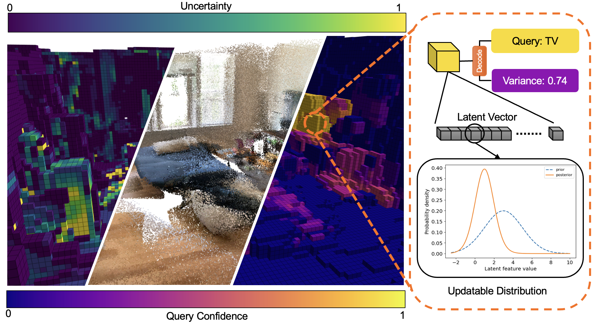
Figure 1: LatentBKI enables semantic mapping by leveraging open-dictionary language inference with vision-language (VL) model data. VL networks process exteroceptive data to generate point-wise features, which LatentBKI integrates into a 3D map via Bayesian Kernel Inference (BKI). Unlike prior VL mapping methods, LatentBKI updates nearby voxels using spatial information and maintains quantifiable uncertainty via conjugate priors. As shown, LatentBKI applies to real-world scenes (middle), quantifies semantic uncertainty per voxel (left), and decodes voxel features into categories using the VL network’s language-driven decoder (right).

Recently, deep learning has produced foundation models trained on large, varied data sets with the reported ability to generalize to out-of-distribution data, solving a limitation of previous semantic segmentation neural networks [4, 5, 6]. Additionally, such open-dictionary segmentation networks can share a feature space with large language models [7], creating a class of networks known as Vison-Language (VL) models [8]. While several methods for VL mapping have been proposed, classical robotic challenges of continuous mapping and quantifying uncertainty remain.

Quantifying uncertainty is critical for robotics applications, as observations of the world are limited and noisy, both from sensor noise as well as neural network errors. Probabilistic mapping seeks to quantify uncertainty in the world model by tracking the number of observations of the environment, as well as the variance or stochasticity of the observations. Additionally, in practice, observations of the environment may be sparse, leading to incomplete maps.

Completing maps from sparse data is known as the task of scene completion, which seeks to leverage exteroceptive information to form a more complete scene. While one branch of scene completion seeks to complete maps implicitly through neural networks [9, 10], a probabilistic approach to scene completion is known as continuous mapping, which leverages spatial observations to complete representations of the environment [11]. One benefit of continuous mapping is quantifiable uncertainty, as the influence of points in the map is modeled through spatial relationships. However, continuous semantic mapping has been limited to closed-dictionary categorical spaces, which is impractical for complex environments.

This paper proposes an extension of continuous mapping to the latent space of neural networks, enabling open-dictionary continuous mapping. The proposed method, LatentBKI, performs Bayesian Kernel Inference (BKI) [12] over the latent embedding space to probabilistically complete scenes from sparse data with quantifiable uncertainty through conjugate priors. We compare our method against the pioneering work VL-Map, which introduced a method for mapping in a latent space from VL networks but does not quantify uncertainty or leverage spatial relations. We also compare our method against closed-dictionary continuous mapping methods, demonstrating that our method enables open-dictionary mapping without losing performance and with similar abilities to quantify uncertainty. Finally, we evaluate our method on real-world indoor scenes, highlighting the advantage of leveraging open-dictionary segmentation networks for continuous mapping. To summarize, our contributions are:

1. Novel mapping algorithm which extends continuous Bayesian Kernel Inference (BKI) to latent spaces.

2. Spatial smoothing and uncertainty quantification through conjugate priors in VL maps.

3. Demonstration of segmentation and uncertainty quantification in real-world environments.

4. Open-source software is available for download at https://github.com/UMich-CURLY/LatentBKI.

II Related Work

We review the literature on semantic mapping using continuous probabilistic inference, which creates comprehensive maps with quantifiable uncertainty but is limited to predefined categories. We then examine VL networks and maps, which allow for open-dictionary segmentation at inference time. LatentBKI addresses the challenge of integrating continuous probabilistic mapping with VL networks.

II-A Continuous Semantic Mapping

Robots require advanced levels of scene understanding to plan, including knowledge of the geometry and semantic labels of objects and uncertainty associated with the objects to avoid failure due to mistaken object identity. Often, these approaches use task-dependent object designations as semantic labels [13, 14] such as abstract topological information [15] or material classifications [16]. State-of-the-art methods for semantic classification almost exclusively rely on neural networks to produce pixel-wise semantic predictions [17, 18, 19]. Neural networks can successfully categorize objects. Robotics research has focused on incorporating segmentation predictions into maps via semantic label fusion [20, 21]. Recent methods aim to quantify uncertainty through Bayesian inference [22, 23] by iteratively fusing semantic estimates projected onto a geometric map.

Kernel-based inference schemes have had notable success [24, 25] in probabilistic semantic mapping. Bayesian Kernel Inference (BKI), proposed by [12], approximates the spatial influence of points at model selection through the usage of a kernel. BKI is an approximation of Gaussian Processes, which are effective at continuous mapping yet suffer from a cubic computational complexity [11, 26, 27]. Effectively, the kernel defines the shape or distribution of a point, deemed the extended likelihood, and can be applied to create an efficient, closed-form Bayesian update with more complete maps and quantifiable uncertainty [28]. While BKI has been applied effectively to semantic mapping [29, 25, 30], semantic maps are inherently limited to a closed set of pre-specified categories. In contrast, we propose to extend the literature of continuous mapping to the latent space of neural networks, allowing for open-vocabulary inference within the latent space of VL models.

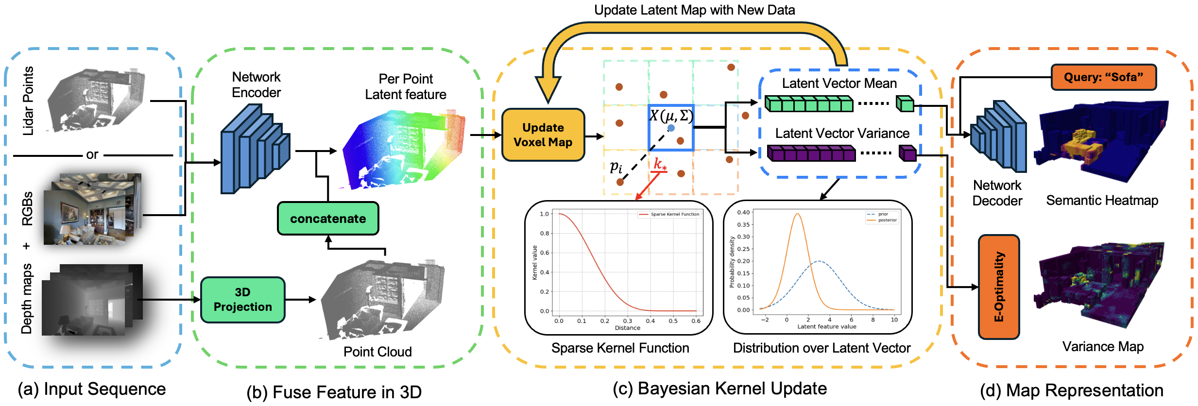
Figure 2: This demonstrates the overall pipeline of LatentBKI. (a) The input to LatentBKI is 3D points, which can be from LiDAR, RGB-D, or any exteroceptive sensor with 3D input. (b) Points are then processed by an off-the-shelf neural network, which encodes each point into a latent space. (c) By adopting a Gaussian likelihood over the point-wise features, we perform closed-form Bayesian inference on a voxel map where each voxel contains parameters modeling the conjugate prior of the multivariate Gaussian distribution. Additionally, instead of only considering points which fall within a voxel, we consider nearby points weighted through a kernel function. (d) The posterior predictive distribution of each voxel in latent space can then be decoded using the decoder of the neural network, enabling the computation of open-dictionary segmentation predictions with expectation and uncertainty.

II-B Vision Language Mapping

Rapidly improving Large Language Models (LLMs) demonstrating remarkable generalizable capabilities have motivated the advent of vision-language models (VLM) with shared latent space for both images and texts [8]. The pioneering method CLIP successfully represents visual and textual information in the same embedding dimension through contrastive learning [6]. Trained on a large dataset of image-text pairs, CLIP learns embed features from visual or textual information in a shared feature space, where similarity is measured by a cosine similarity function [6]. Several following works have improved upon the data efficiency of CLIP [31] and image contextualization [32].

Based on the success of VLMs and their great zero-shot performance, recent robotics research has focused on open-dictionary mapping which operates in the latent space of VLMs and can create segmentation predictions from language descriptors [7]. Approaches like LM-Nav [33], CoW [34], NLMap [35] have fused VLMs to enable robots to understand and navigate new environments. One of the pioneering approaches is VLMaps [36], which showed outstanding performance on zero-shot navigation tasks. It uses the language-driven semantic segmentation network LSeg [7] to generate feature embeddings for pixels in images the robot observes. Pixel-wise latent embeddings are then stored in a 3D voxel map through a weighted averaging scheme, where weights are dependent on pixel depths and points at extreme distances are excluded [37, 38]. The latent expectation of each voxel can then be decoded into per-category scores given the language embeddings of a set of categories, thereby enabling open-dictionary queries. While successful, this approach loses the ability to quantify uncertainty and fill in gaps in the map from probabilistic continuous mapping, as discussed previously. Therefore, we propose to extend closed-dictionary continuous semantic mapping to open-dictionary VL maps.

III Method

We propose a novel method for probabilistic continuous mapping in the feature space of neural networks, which recurrently incorporates predictions from neural networks to learn an expectation and variance. Our mapping framework, which we call LatentBKI, has applications for general deep neural networks and is especially powerful when combined with modern foundation models such as VL models. Compared to previous methods which map in an explicit categorical space, continuous mapping in the feature space allows for open-dictionary queries with quantifiable uncertainty. A diagram of our method is shown in Fig. 2, demonstrating the ability of LatentBKI to complete scenes, decode semantic information, and quantify uncertainty in the latent space.

LatentBKI is built on the intuition that neural network features are geometrically continuous and suitable for kernel methods. Interpolation is a common step in modern neural networks to infer features from geometrically adjacent points, used especially in upsampling or deformable operations. Interpolation of point $x$ on feature grid $G$ with height $H$ and width $W$ can be written as:

$$G_{x}\approx\frac{\sum_{i=1}^{H}\sum_{j=1}^{W}w_{ij}G_{ij}}{\sum_{i}\sum_{j}w_{ij}}$$ (1)

where $i$ and $j$ are indices of neighboring cells, and weights $w$ are determined by the distance of query point $x$ to neighboring cells. This equation resembles the Nadaraya-Watson kernel estimate of the expected value, written similarly as:

$$\hat{G_{x}}=\frac{\sum_{i=1}^{N}k(x-x_{i})G_{i}}{\sum_{i=1}^{N}k(x-x_{i})}$$ (2)

for a set of $N$ data points. As we will show next, our method produces an expectation equivalent to the Nadaraya-Watson kernel estimate, with the addition of quantifiable uncertainty through conjugate priors.

III-A Latent Mapping Representation

Our map representation consists of a voxel map with voxels $*$ located at position $x_{*}$. At each time-step our map is provided a set of points $\mathcal{D}=\{(x_{i},y_{i})\}_{i=1}^{N}$, where $x_{i}\in\mathbb{R}^{3}$ is the position of point $i$ and $y_{i}\in\mathbb{R}^{C}$ is the corresponding latent feature of point $i$. From these points, our goal is to probabilistically update the latent parameters of each voxel, $y_{*}$, to obtain the posterior.

In order to accomplish this goal, we first define a Gaussian likelihood over the feature space, such that:

$$p(y_{i}|\mu_{i},\Sigma_{i})=\mathcal{N}(y_{i};\mu_{i},\Sigma_{i}).$$ (3)

Since the features originate from a neural network, the likelihood defines an unknown expectation and variance which the point’s features are sampled from. Similarly, we can define the points observed within a voxel $*$ according to the same likelihood distribution. From the likelihood, we can write an expression for the posterior of the latent parameters $\theta_{*}=\{\mu_{*},\Sigma_{*}\}$ of voxel $*$ using Bayes’ rule as:

$$p(\theta_{*}\mid x_{*},\mathcal{D})\propto p(\mathcal{D}\mid\theta_{*},x_{*})p(\theta_{*}\mid x_{*}).$$ (4)

In order to model the distribution over the parameters $\theta_{*}$ of the voxel, which themselves define a multivariate Gaussian distribution, we adopt the conjugate prior of the multivariate Gaussian distribution, the normal-inverse Wishart distribution. The normal-inverse Wishart distribution defines a distribution over the multivariate Gaussian with unknown mean $\mu_{*}$ and covariance $\Sigma_{*}$ through parameters $\mu^{\prime}_{*},\Psi_{*},\lambda_{*},v_{*}$ as:

$$p(\mu_{*},\Sigma_{*})=\mathcal{N}\left(\mu_{*};\mu^{\prime}_{*},\frac{\Sigma_{*}}{\lambda_{*}}\right)\cdot\mathcal{W}^{-1}(\Sigma;\Psi_{*},v_{*}),$$ (5)

where the hyper-parameters represent the prior expectation of the mean ($\mu^{\prime}_{*}$), the expectation of the covariance ($\Psi_{*}$), and the confidence in the mean and covariance estimates ($\lambda_{*},v_{*}$). In our case, $\lambda_{*}$ and $v_{*}$ are equal and correspond to weighted counts of the total observations.

Although the conjugate prior provides a closed-form solution for updating the multivariate normal distribution parameters for each voxel, it does not consider the spatial locations of points. Intuitively, points that are closer to the centroid of the voxel should have a higher influence, while points that are further from the voxel centroid should have a lower influence. Additionally, only updating the voxels which points fall into can lead to sparse maps, as previously noted. Therefore, we adopt the solution of [12], which defines an extended likelihood distribution that considers the spatial relationship of points to voxels through the use of a kernel function $k(x_{i},x_{*})$ as:

$$p(y_{i}|x_{i},\theta_{*},x_{*})\propto p(y_{i}|\theta_{*})^{k(x_{i},x_{*})}.$$ (6)

The only requirements when defining the extended likelihood are that

$$k(x,x)=1\,\forall\,x\quad\text{and}\quad k(x,x_{*})\in[0,1]\,\forall\,(x,x_{*}).$$ (7)

Applied to the previously defined Gaussian likelihood, the extended likelihood can be written as:

$$p(y_{i}|\theta_{*},x_{i},x_{*})=\mathcal{N}\left(y_{i};\mu_{*},\frac{\Sigma_{*}}{k(x_{i},x_{*})}\right).$$ (8)

Effectively, observations close to the voxel centroid have lower variance than observations of further points, resulting in more influence or gain. Following Semantic BKI, we use a symmetric sparse kernel [39] as the kernel function for direct comparison. Substituting the extended likelihood into (4), we can now define a spatial update over the voxel parameters as:

$$p(\theta_{*}|x_{*},y_{1:N},x_{1:N})\propto\left[\prod_{i=1}^{N}p(y_{i}|\theta_{*},x_{i},x_{*})\right]p(\theta_{*}|x_{*}).$$ (9)

Next, we present our map update algorithm, which follows the closed-form solution derived by [12].

III-B Latent Mapping Update

First, we initialize the confidence over the mean and covariance of each voxel to a non-informative value of $\lambda_{*}\approx 0$. As points are observed, the value of $\lambda_{*}$ increases, indicating more confidence in the expected mean and covariance of the voxel. At time-step $t$, voxels are parameterized by prior $\mu_{*}^{t-1}$, $\Psi_{*}^{t-1}$ and confidence $\lambda_{*}^{t-1}$, with input points $\mathcal{D}$.

The influence of the new observations is calculated by:

$$\bar{k}_{*}=\sum_{i=1}^{N}k(x_{*},x_{i}),$$ (10)

where the kernel function measures the influence of point $i$ over voxel $*$. The confidence in the mean and covariance is updated:

$$\lambda_{*}^{t}=\lambda_{*}^{t-1}+\bar{k}_{*}.$$ (11)

Input observations are then used to compute the new mean as a running average:

$$\bar{y}_{*}=\sum_{i=1}^{N}\frac{k(x_{*},x_{i})}{\bar{k}_{*}}y_{i},\quad\mu_{*}^{t}=\frac{\lambda_{*}^{t-1}\mu_{*}^{t-1}+\bar{y}_{*}\bar{k}_{*}}{\lambda_{*}^{t}}.$$ (12)

Remark 1.

We note that the formulation of the new mean resembles the Nadaraya-Watson estimate mentioned in Section III-A, as input features are weighted by the kernel function to obtain a weighted average.

Last, following [12], we update the expected covariance by weighting the covariance of the newly observed points:

$$\bar{E}_{*}=(\bar{y}_{*}-\mu_{*}^{t-1})(\bar{y}_{*}-\mu_{*}^{t-1})^{T},$$ (13)

$$\bar{S}_{*}=\sum_{i=1}^{N}k(x_{i},x_{*})(y_{i}-\bar{y}_{*})(y_{i}-\bar{y}_{*})^{T},$$ (14)

$$\Psi*^{t}=\Psi*^{t-1}+\bar{S}_{*}+\frac{\lambda_{*}^{t-1}\bar{k}_{*}}{\lambda_{*}^{t}}\bar{E}_{*}.$$ (15)

As new points are obtained, the above process is repeated to update the mean, covariance, and confidence level. For simplicity, we assume a diagonal covariance, which significantly reduces the number of parameters stored per voxel. Diagonal covariances are common in the feature space and are used in variational auto-encoders (VAEs).

III-C Inference

After updating the map, we can compute an expectation and variance for features observed within each voxel. First, the distribution can be marginalized to obtain a posterior predictive solution that defines the probability of observing a feature $y_{*}$ at voxel centroid $x_{*}$. The posterior predictive distribution for voxel $*$ is:

$$p(y_{*}|x_{*})=t_{\lambda_{*}}\left(\mu_{*},\frac{\lambda_{*}+1}{\lambda_{*}^{2}}\Psi_{*}\right),$$ (16)

where $t_{\lambda_{*}}$ is the multivariate Student-$t$ distribution. The multivariate Student-$t$ distribution has an expectation of: $\mathbb{E}(y_{*})=\mu_{*}$, when $\lambda_{*}>1$, and a variance of: $\text{Var}(y_{*})=\frac{\lambda_{*}}{\lambda_{*}-2}\Psi_{*}$, for $\lambda_{*}>2$. However, both the expectation and variance are within the latent space of the neural network and must be decoded to obtain a meaningful interpretation.

When performing open-dictionary inference, the input is a set of phrases $W$ defining semantic categories, which are processed by a language model to obtain text embeddings $F_{w}\in\mathbb{R}^{C}$ per phrase $w\in W$. Specifically, in our experiment, we encode each phrase $w$ as a Clip feature vector $F_{w}$ of 512 length: $F_{w}=\text{Encoder}(w)$. Inspired by LSeg, we obtain the categorical prediction $\hat{w}$ as:

$$\hat{w}=\mathrm{arg\,max}_{w}\,\frac{F_{w}^{\mathsf{T}}\mu_{*}}{\lVert\mu_{*}\rVert_{{}_{2}}\lVert F_{w}\rVert_{{}_{2}}}.$$ (17)

Remark 2.

We note that while we present the decoding for open-dictionary queries, LatentBKI can be decoded into any format using neural network decoders.

III-D Uncertainty Quantification

While the map update step described above can propagate uncertainty, the variance is limited to the latent space of the neural network encoder. Therefore, we propose two methods to quantify uncertainty.

First, following the approach of other neural network uncertainty quantification methods, we propose quantifying uncertainty through sampling. To quantify uncertainty through sampling, we sample many realizations of the voxel feature $y_{*}$, which we decode through the neural network decoder. Then, we compute the variance of the predictions in the decoded space. While this approach is accurate, it requires extra computation, which we propose to avoid.

Based on a common approach of information quantification in optimal experimental design [40], we can quantify uncertainty through p-optimality [41]. Although p-optimality leads to many solutions [42], in this work, we compute the uncertainty $U_{*}$ via E-optimality criterion as:

$$U_{*}=\max\left(\text{Var}(y_{*})\right),$$ (18)

and the uncertainty via D-optimality criterion as:

$$U_{*}=\exp\left(\frac{\sum_{i=1}^{C}\log\left(\text{Var}(y_{*})_{i}\right)}{C}\right),$$ (19)

where a large value corresponds to high uncertainty. This is because, experimentally, we find that E-optimality is highly correlated with the sampling-based uncertainty and is quick to compute. See Section IV-C for detailed experiments.

IV Results and Discussion

We quantitatively and qualitatively show that LatentBKI effectively extends the continuous probabilistic mapping literature to neural network latent spaces, bringing quantifiable uncertainty and spatial smoothing to VL maps. First, we compare LatentBKI against closed-dictionary continuous mapping to verify that operations in the latent space of neural networks do not affect mapping performance. Next, we compare LatentBKI against VLMap, which performs latent space mapping but does not leverage spatial information or quantify uncertainty. Third, we study the correlation of our uncertainty quantification with segmentation errors and the effect of spatial smoothing. Finally, we conduct real-world experiments to demonstrate the ability of our map to transfer to real-world open-dictionary scenarios due to the strong generalization capabilities of large VL networks.

Table I: Comparison against closed-dictionary BKI mapping.

Data	Method	Acc. $(\%)$	mIoU $(\%)$	Queries
Indoor	Segmentation	66.20	20.95	N/A
	ConvBKI (Single)	68.87	24.28	Fixed
	LatentBKI	68.16	23.14	Open
Outdoor	Segmentation	90.46	52.05	N/A
	ConvBKI (Single)	91.01	56.38	Fixed
	LatentBKI	91.29	57.33	Open

IV-A Comparison against categorical space mapping method

First, we compare LatentBKI against the closed-dictionary semantic mapping method defined in [29], which leverages BKI with a categorical likelihood to update the map. Specifically, we compare against ConvBKI [25] using a single un-trained spherical kernel for direct comparison. Our goal of this study is to verify that LatentBKI can generalize BKI into the latent space of neural networks without any significant changes in performance.

We evaluate LatentBKI and ConvBKI (single) on an indoor and outdoor dataset. For the indoor dataset, we use Matterport3D (MP3D) [43] with an image semantic segmentation network, Language-driven Semantic Segmentation (LSeg) [7]. For the outdoor dataset, we choose the Semantic KITTI dataset [44] and use the Sparse Point-Voxel Convolution Neural Network (SPVCNN) [45, 46] for point cloud semantic prediction. Since the latent space of LSeg has a large dimension of 512, we use Principal Component Analysis (PCA) to down-sample features for the map update. The PCA algorithm is trained on held-out MP3D sequences we do not compare with ConvBKI on, and we experimentally find that reducing the size of the latent space of LSeg to 64 results in only a $0.09\%$ loss in accuracy and $0.42\%$ decrease in mIoU.

We apply the same configuration to both mapping algorithms to ensure comparable results. Each algorithm uses a voxel resolution of 0.1 meters, a sparse kernel with a kernel length of 0.5 meters, and a filter size of 3, determining how many neighboring voxels should be updated for a single-point observation. We apply a cubic filter in this case, so $3^{3}=27$ neighboring voxels will be considered. Since both methods compare spatial smoothing, we provide 80% of the points as input and evaluate semantic predictions over the mean intersection over union (mIoU) and accuracy metrics on the remaining 20% of the points.

As shown in Table I, LatentBKI performs similarly to ConvBKI over indoor and outdoor datasets. These results verify that BKI with a Gaussian likelihood is suitable for the latent space of multiple neural networks and does not cause any significant changes in performance. While LatentBKI results in a marginal improvement in quantitative performance on the outdoor data, the slight decrease in indoor data is due to the dimensionality reduction applied by PCA on the input to LatentBKI. Additionally, although the studies are performed on closed-dictionary segmentation, LatentBKI enables open-dictionary continuous mapping as the per-voxel latent features can be decoded into more meaningful outputs, which we demonstrate in Section IV-D. Next, we compare LatentBKI with a popular latent mapping algorithm, VLMap.

IV-B Latent Mapping Comparison

We compare LatentBKI with a similar open-dictionary mapping method VLMap [36], which also updates voxels through a weighted averaging approach. Since VLMap does not utilize spatial information, we compare LatentBKI to VLMap with a filter size of 1, disregarding points in nearby voxels when calculating the posterior state of a voxel. Both methods use the open-dictionary encoder LSeg, with features downsampled by PCA to a latent size of $64$.

We compare each method on the MP3D dataset [43] following the same experimental setup as VLMap, including a resolution of $0.05$ m to account for the fine-resolution indoor environment. To ensure that the input and evaluation points are consistent, we implemented the pre-processing heuristics of VLMap within our method. These heuristics include discarding pixels with extreme depths, discarding points outside of the scene range, and downsampling input points. Specifically, the same set of $1\%$ of remaining pixels are provided to each method, and points with depth less than $0.1$ meters or greater than $6$ meters are excluded. By following the same downsampling heuristics as VLMap in our evaluation, we isolate the effect of the sparse kernel function used by our method to weight input points compared to the depth-wise weighting scheme employed by VLMap.

The results of our experiments on two different MP3D sequences, as shown in Table II, indicate that LatentBKI outperforms VLMap in both accuracy and mean IoU, which we attribute to the sparse kernel. At its core, the VLMap algorithm is similar to our method of calculating the expectation with a different weighting scheme, and without spatial smoothing or quantifiable uncertainty. This performance improvement may be attributed to the formalized mathematical updates in LatentBKI, which provide a more robust integration of observations and better handling of uncertainty. Additionally, the formal probabilistic approach we leverage in LatentBKI allows for quantifiable uncertainty, which we study next.

Table II: Comparison against VLMap, which performs latent mapping without spatial smoothing or uncertainty quantification. Results are compared on scenes gTV8FGcVJC9 (1) and 5LpN3gDmAk7 (2) of MP3D.

Scene	Method	Acc. $(\%)$	mIoU $(\%)$	Uncertainty
1	Segmentation	61.08	19.57	N/A
	VLMap	60.94	20.32	No
	LatentBKI	63.30	21.56	Yes
2	Segmentation	63.27	13.12	N/A
	VLMap	64.12	12.44	No
	LatentBKI	66.10	14.92	Yes

IV-C Ablation Studies

Two benefits of LatentBKI are the spatial smoothing effect of continuous mapping and the ability to quantify the temporal uncertainty of neural network predictions. In this section, we study the quantitative improvement from different kernel sizes, as well as compare the sampling and P-Optimality methods for quantifying uncertainty.

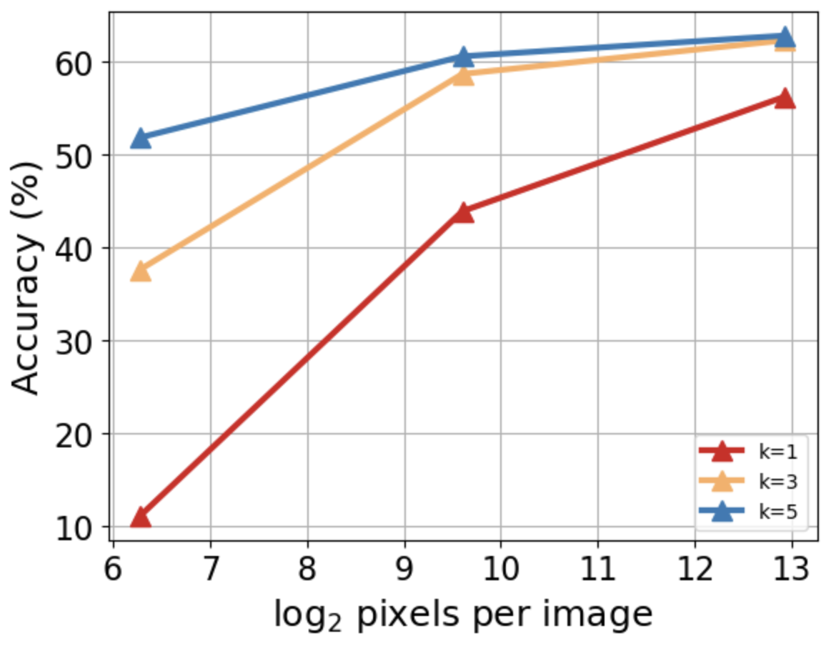
(a) Accuracy vs. Input Sparsity

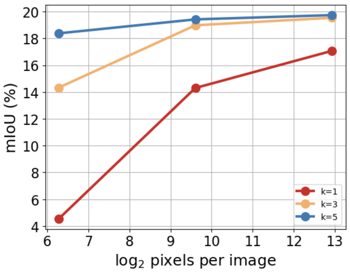
(b) mIou vs. Input Sparsity

Figure 3: Effect of spatial smoothing with varying levels of image sparsity. Spatial smoothing, indicated by the filter size $k$, is most effective for sparse images. The original image has a resolution of $720$ by $1080$ pixels.

Spatial Smoothing: In real-world applications, data is often sparse due to sensors such as LiDAR or sparse stereo matching algorithms. BKI provides a probabilistic technique to create more complete maps from sparse spatial data by leveraging the spatial smoothing effect of kernels. In this experiment, we compare different kernel sizes and their ability to complete the map from sparse data.

All kernels are compared on the same scene of MP3D, where data is downsampled temporally to incorporate only one in 3 frames and at the image level to use a randomly sampled set of pixels from each image. Fig. 3 demonstrates plots of the segmentation performance of different kernel sizes and varying sparsity levels. At extreme sparsity levels, spatial smoothing of points benefits the map completeness. As the input becomes more dense, in this case, due to high-resolution images with accurate depth, the effect of the kernel is diminished.

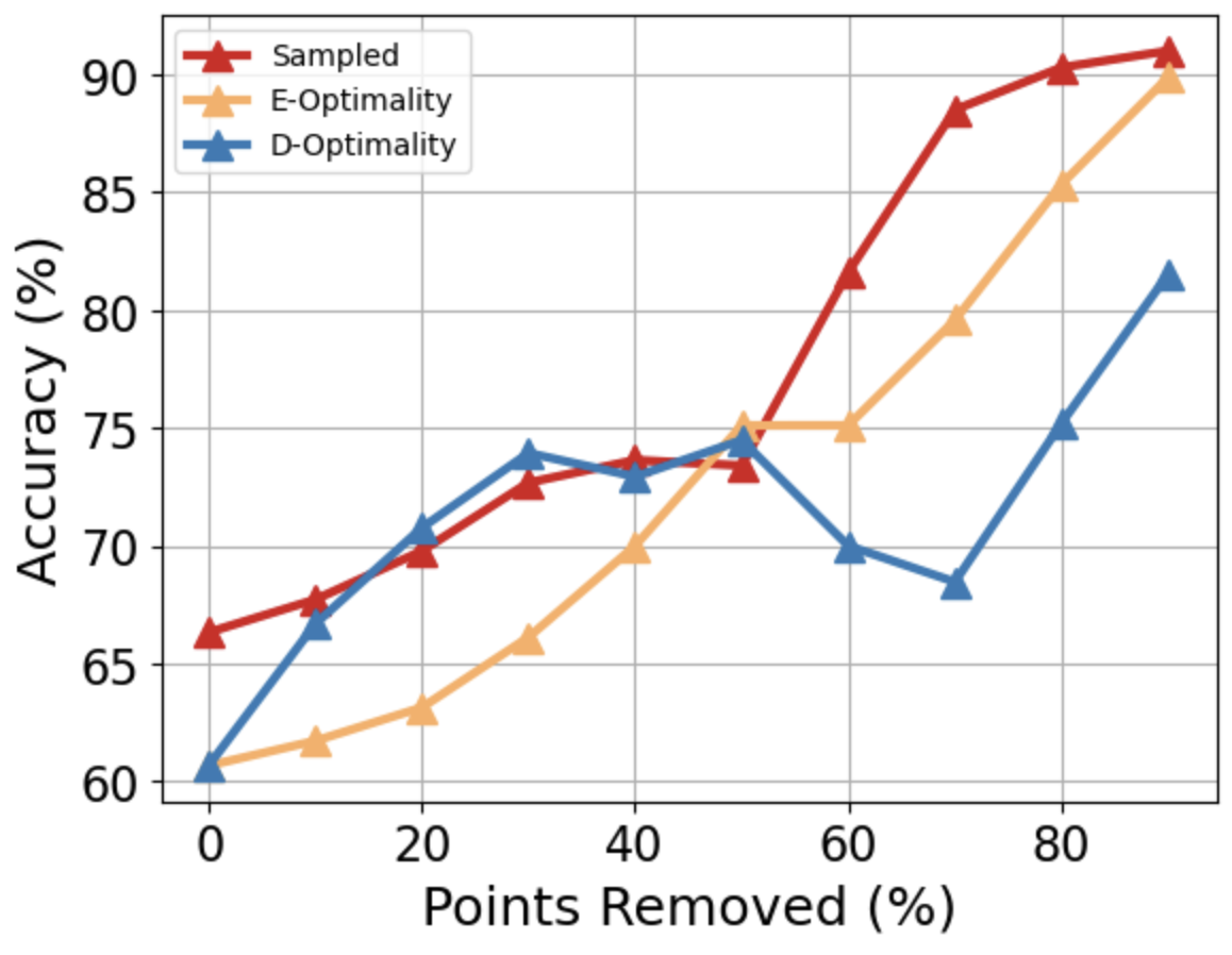
(a) Accuracy vs. uncertainty

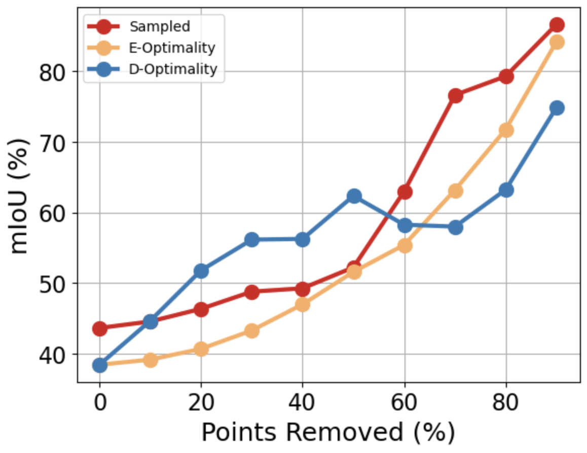
(b) mIou vs. uncertainty

Figure 4: Sparsification plot of segmentation performance compared to quantified uncertainty. As uncertain points are removed, a well calibrated uncertainty should cause the segmentation performance to increase.

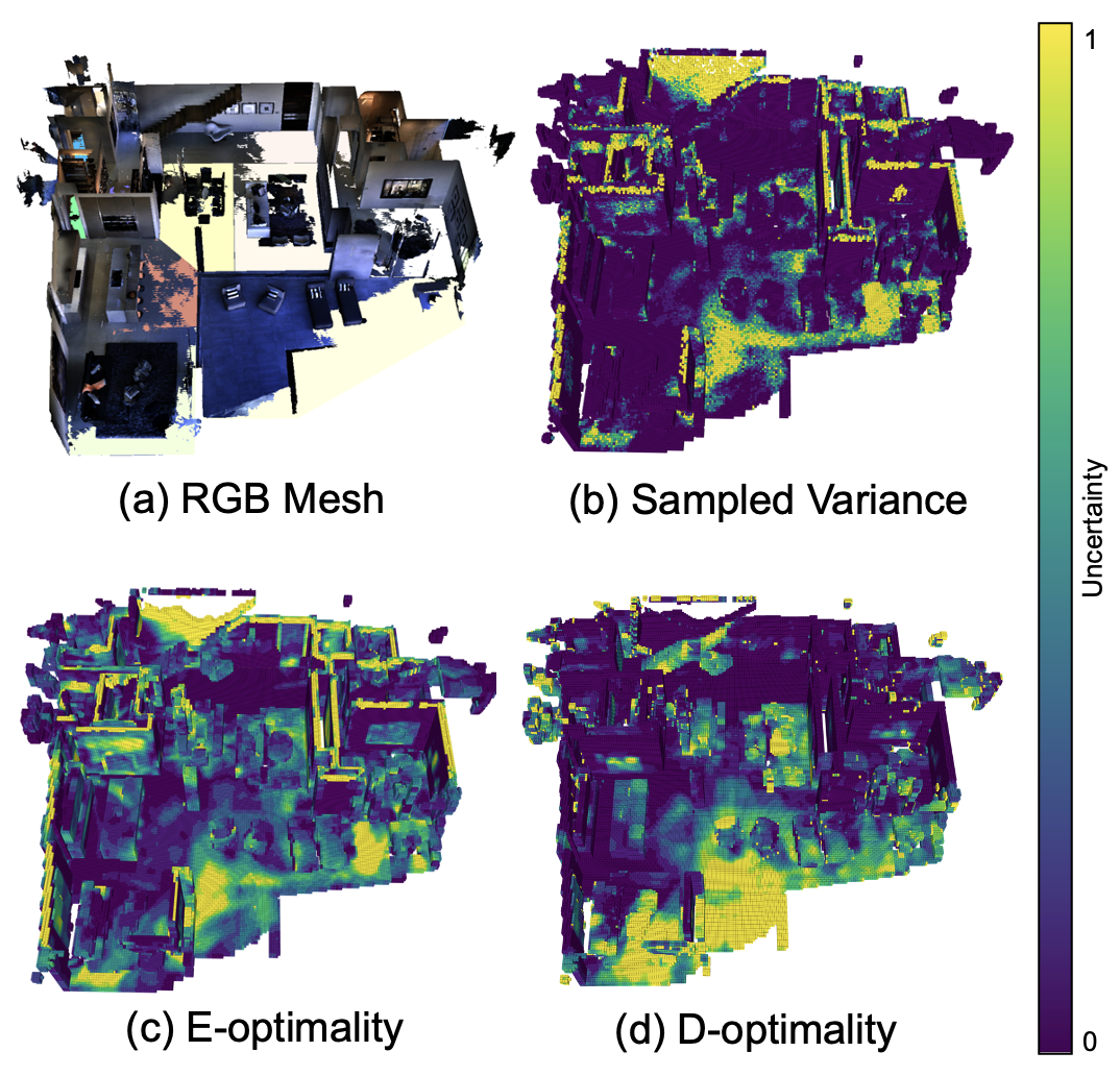
Figure 5: Uncertainty maps for 5LpN3gDmAk7 MP3D sequence. (a) Covered house mesh in the sequence. (b) Categorical variance map by sampling from distribution. (c) Variance map by using E-optimality in latent space. (d) Variance map by using D-optimality in latent space.

Uncertainty Quantification: To evaluate the ability of LatentBKI to quantify uncertainty meaningfully, we quantitatively and qualitatively compare uncertainty quantification on the MP3D dataset using LSeg as the encoder. We construct a map using LatentBKI, then compare uncertainty quantified using D-optimality, E-optimality, and sampling as described in Section III-D. Whereas the sampling-based method is commonly used, it is computationally expensive compared to the E-optimality and D-optimality-based techniques.

To quantitatively compare each uncertainty quantification method, we create sparsification plots [47] identifying the correlation between uncertainty and prediction error, shown in Fig. 4. To create the sparsification plots, we sort points in a test set by the predicted uncertainty. Next, we separate the sorted points into bins and iteratively remove the most uncertain bin. If the uncertainty is properly calibrated, we expect to see an increase in the accuracy as uncertain points are removed. As seen in Fig. 4, both the accuracy and mIoU metrics are correlated with all three methods, especially sampling and E-optimality. In addition to a strong correlation between latent uncertainty and error in the decoded predictions, E-optimality benefits from efficient computation.

We also qualitatively compare uncertainty quantification between sampling and E-optimality, shown in Fig. 5. We observe that the most uncertain voxels are typically located at the edges of rooms or at objects that are difficult for the VL network to identify due to ambiguity or poorly captured images. Similar to the sparsification plots, we find that E-optimality closely aligns with the uncertainty estimated through sampling, indicating that E-optimality is an effective approximation for the latent uncertainty.

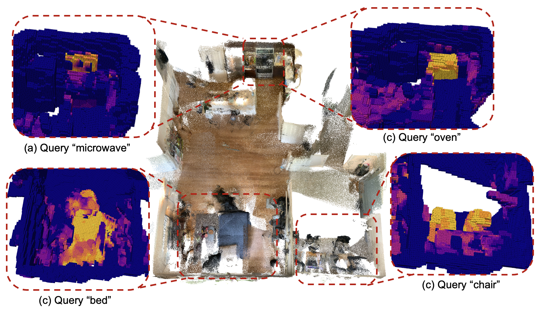
Figure 6: Open vocabulary query task results. Query results are shown in heat map, brighter colors indicates higher values.

IV-D Real-World Experiment

To show that LatentBKI can generalize to real-world settings, we use an iPad with a 3D recording software, Record3D, to collect RGB-D data and camera poses of indoor scenes for mapping. We process the images with LSeg, and create a map of a real-world apartment using LatentBKI, shown in Figure 6.

In Fig. 6, we demonstrate how Latent-BKI enables open-vocabulary queries which are more suitable for complex indoor environments. In this figure, we query arbitrary words in the map and portray a heat map of the voxels corresponding to the query word. While results were compared on a closed set of segmentation categories, our method enables language-based inference with quantifiable uncertainty. This is especially important because indoor environments can contain infinitely many categories of objects that cannot be captured adequately with a pre-specified set of objects.

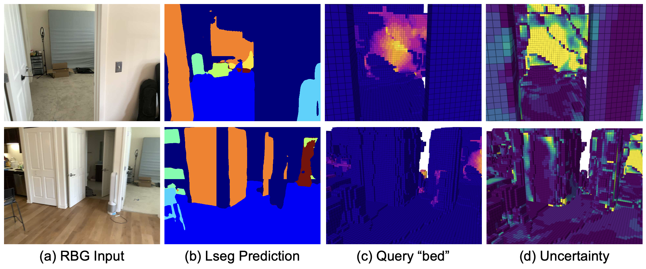
Figure 7: The first column (a) shows RGB input across different frames containing “bed”. Column two (b) shows the Lseg network semantic prediction result, which gives inconsistent wrong semantic prediction across frames. Later two columns, (c) shows the heatmap of the query result of “bed” and (d) show the uncertainty. Our method shows a consistently high probability in the same area for the “bed” while maintaining the knowledge that the observations on the “bed” area are noise by showing high uncertainty.

An additional benefit of LatentBKI is the ability to quantify uncertainty, which we demonstrate in Fig. 7. The input segmentation network has difficulty identifying a vertically placed mattress, producing inconsistent embeddings across different views. As a result, this region of the map exhibits high variance. Although the network prediction is noisy, Latent BKI can generate consistent query results for “bed” while acknowledging the high uncertainty from the network in that area.

V Conclusion

We introduced LatentBKI, a novel method for probabilistically updating a voxel map where each voxel stores a latent descriptor in the embedding space of foundation models with quantifiable uncertainty. LatentBKI extends the classical literature of continuous semantic mapping to open-dictionary mapping, enabling language-based queries while maintaining quantifiable uncertainty. Language-based queries can handle the complexities posed by real-world robotic applications that may contain detailed environments and require human interaction.

While LatentBKI demonstrated success in open-dictionary environments through a Gaussian likelihood, there are several avenues for future work. First, LatentBKI does not consider the unique geometry of objects and can therefore be combined with architectures such as ConvBKI, which learns per-category kernels, or the high-quality 3D Gaussian Splatting [48] novel view synthesis method which represents the environment using 3D ellipsoids, similar to the kernel structure we leverage for continuous mapping. Additionally, inspired by the recent work on open-dictionary radiance fields [49], we believe that the segment anything model [4, 5] may be useful when identifying the boundaries of objects.

References

- [1] S. Casas, A. Sadat, and R. Urtasun, “MP3: A Unified Model to Map, Perceive, Predict and Plan,” in Proc. IEEE Conf. Comput. Vis. Pattern Recog., 2021, pp. 14 403–14 412.
- [2] H. L. Chiang, A. Faust, M. Fiser, and A. Francis, “Learning Navigation Behaviors End-to-End With AutoRL,” IEEE Robot. Autom. Letter., vol. 4, no. 2, pp. 2007–2014, 2019.
- [3] H. Moravec and A. Elfes, “High resolution maps from wide angle sonar,” in Proc. IEEE Int. Conf. Robot. and Automation, vol. 2, 1985, pp. 116–121.
- [4] A. Kirillov, E. Mintun, N. Ravi, H. Mao, C. Rolland, L. Gustafson, T. Xiao, S. Whitehead, A. C. Berg, W.-Y. Lo, P. Dollar, and R. Girshick, “Segment anything,” in Proc. IEEE Conf. Comput. Vis. Pattern Recog., October 2023, pp. 4015–4026.
- [5] N. Ravi, V. Gabeur, Y.-T. Hu, R. Hu, C. Ryali, T. Ma, H. Khedr, R. Rädle, C. Rolland, L. Gustafson, E. Mintun, J. Pan, K. V. Alwala, N. Carion, C.-Y. Wu, R. Girshick, P. Dollár, and C. Feichtenhofer, “SAM 2: Segment Anything in Images and Videos,” 2024.
- [6] A. Radford, J. W. Kim, C. Hallacy, A. Ramesh, G. Goh, S. Agarwal, G. Sastry, A. Askell, P. Mishkin, J. Clark, G. Krueger, and I. Sutskever, “Learning Transferable Visual Models From Natural Language Supervision,” in Proc. Int. Conf. Machine Learning, ser. J. Mach. Learning Res., M. Meila and T. Zhang, Eds., vol. 139. PMLR, 18–24 Jul 2021, pp. 8748–8763.
- [7] B. Li, K. Q. Weinberger, S. Belongie, V. Koltun, and R. Ranftl, “Language-driven Semantic Segmentation,” in Proc. Int. Conf. Learning Representations, 2022.
- [8] J.-B. Alayrac, J. Donahue, P. Luc, A. Miech, I. Barr, Y. Hasson, K. Lenc, A. Mensch, K. Millican, M. Reynolds et al., “Flamingo: a visual language model for few-shot learning,” Proc. Advances Neural Inform. Process. Syst. Conf., vol. 35, pp. 23 716–23 736, 2022.
- [9] L. Roldao, R. de Charette, and A. Verroust-Blondet, “3D Semantic Scene Completion: a Survey,” Int. J. Comput. Vis., 2022.
- [10] J. Wilson, J. Song, Y. Fu, A. Zhang, A. Capodieci, P. Jayakumar, K. Barton, and M. Ghaffari, “MotionSC: Data Set and Network for Real-Time Semantic Mapping in Dynamic Environments,” IEEE Robot. Autom. Letter., vol. 7, no. 3, pp. 8439–8446, 2022.
- [11] S. T. O’Callaghan and F. T. Ramos, “Gaussian process occupancy maps,” Int. J. Robot. Res., vol. 31, no. 1, pp. 42–62, 2012.
- [12] W. R. Vega-Brown, M. Doniec, and N. G. Roy, “Nonparametric Bayesian inference on multivariate exponential families,” in Proc. Advances Neural Inform. Process. Syst. Conf., Z. Ghahramani, M. Welling, C. Cortes, N. Lawrence, and K. Q. Weinberger, Eds., vol. 27. Curran Associates, Inc., 2014.
- [13] J. Deng, W. Dong, R. Socher, L.-J. Li, K. Li, and L. Fei-Fei, “Imagenet: A large-scale hierarchical image database,” in Proc. IEEE Conf. Comput. Vis. Pattern Recog. Ieee, 2009, pp. 248–255.
- [14] T.-Y. Lin, M. Maire, S. Belongie, J. Hays, P. Perona, D. Ramanan, P. Dollár, and C. L. Zitnick, “Microsoft coco: Common objects in context,” in Proc. European Conf. Comput. Vis. Springer, 2014, pp. 740–755.
- [15] B. Kuipers and Y.-T. Byun, “A robot exploration and mapping strategy based on a semantic hierarchy of spatial representations,” Robot. and Auton. Syst., vol. 8, no. 1-2, pp. 47–63, 1991.
- [16] P. Upchurch and R. Niu, “A Dense Material Segmentation Dataset for Indoor and Outdoor Scene Parsing,” in Proc. European Conf. Comput. Vis., S. Avidan, G. Brostow, M. Cissé, G. M. Farinella, and T. Hassner, Eds., 2022, pp. 450–466.
- [17] Y. Guo, Y. Liu, T. Georgiou, and M. S. Lew, “A review of semantic segmentation using deep neural networks,” International journal of multimedia information retrieval, vol. 7, pp. 87–93, 2018.
- [18] S. Hao, Y. Zhou, and Y. Guo, “A brief survey on semantic segmentation with deep learning,” Neurocomputing, vol. 406, pp. 302–321, 2020.
- [19] R. Strudel, R. Garcia, I. Laptev, and C. Schmid, “Segmenter: Transformer for semantic segmentation,” in Proc. IEEE Int. Conf. Comput. Vis., 2021, pp. 7262–7272.
- [20] J. McCormac, A. Handa, A. Davison, and S. Leutenegger, “Semanticfusion: Dense 3d semantic mapping with convolutional neural networks,” in Proc. IEEE Int. Conf. Robot. and Automation. IEEE, 2017, pp. 4628–4635.
- [21] N. Sünderhauf, T. T. Pham, Y. Latif, M. Milford, and I. Reid, “Meaningful maps with object-oriented semantic mapping,” in Proc. IEEE/RSJ Int. Conf. Intell. Robots and Syst., 2017, pp. 5079–5085.
- [22] P. Ewen, A. Li, Y. Chen, S. Hong, and R. Vasudevan, “These maps are made for walking: Real-time terrain property estimation for mobile robots,” IEEE Robot. Autom. Letter., vol. 7, no. 3, pp. 7083–7090, 2022.
- [23] P. Ewen, H. Chen, Y. Chen, A. Li, A. Bagali, G. Gunjal, and R. Vasudevan, “You’ve Got to Feel It To Believe It: Multi-Modal Bayesian Inference for Semantic and Property Prediction,” in Robotics. Sci. Sys., 07 2024.
- [24] L. Gan, Y. Kim, J. W. Grizzle, J. M. Walls, A. Kim, R. M. Eustice, and M. Ghaffari, “Multitask learning for scalable and dense multilayer Bayesian map inference,” IEEE Trans. Robot., vol. 39, no. 1, pp. 699–717, 2022.
- [25] J. Wilson, Y. Fu, A. Zhang, J. Song, A. Capodieci, P. Jayakumar, K. Barton, and M. Ghaffari, “Convolutional Bayesian Kernel Inference for 3D Semantic Mapping,” in Proc. IEEE Int. Conf. Robot. and Automation, 2023, pp. 8364–8370.
- [26] M. G. Jadidi, L. Gan, S. A. Parkison, J. Li, and R. M. Eustice, “Gaussian Processes Semantic Map Representation,” ArXiv, vol. abs/1707.01532, 2017.
- [27] J. Wang and B. Englot, “Fast, accurate gaussian process occupancy maps via test-data octrees and nested Bayesian fusion,” in Proc. IEEE Int. Conf. Robot. and Automation, 2016, pp. 1003–1010.
- [28] K. Doherty, T. Shan, J. Wang, and B. Englot, “Learning-Aided 3-D Occupancy Mapping with Bayesian Generalized Kernel Inference,” IEEE Trans. Robot., vol. 35, no. 4, pp. 953–966, 2019.
- [29] L. Gan, R. Zhang, J. W. Grizzle, R. M. Eustice, and M. Ghaffari, “Bayesian Spatial Kernel Smoothing for Scalable Dense Semantic Mapping,” IEEE Robot. Autom. Letter., vol. 5, no. 2, pp. 790–797, 2020.
- [30] J. Wilson, Y. Fu, J. Friesen, P. Ewen, A. Capodieci, P. Jayakumar, K. Barton, and M. Ghaffari, “ConvBKI: Real-Time Probabilistic Semantic Mapping Network with Quantifiable Uncertainty,” IEEE Trans. Robot., pp. 1–20, 2024.
- [31] Y. Li, F. Liang, L. Zhao, Y. Cui, W. Ouyang, J. Shao, F. Yu, and J. Yan, “Supervision Exists Everywhere: A Data Efficient Contrastive Language-Image Pre-training Paradigm,” in Proc. Int. Conf. Learning Representations, 2022.
- [32] L. Yao, R. Huang, L. Hou, G. Lu, M. Niu, H. Xu, X. Liang, Z. Li, X. Jiang, and C. Xu, “FILIP: Fine-grained interactive language-image pre-training,” in Proc. Int. Conf. Learning Representations, 2022.
- [33] D. Shah, B. Osiński, b. ichter, and S. Levine, “LM-Nav: Robotic Navigation with Large Pre-Trained Models of Language, Vision, and Action,” in Conf. Robot. Learning., ser. Proceedings of Machine Learning Research, K. Liu, D. Kulic, and J. Ichnowski, Eds., vol. 205. PMLR, 14–18 Dec 2023, pp. 492–504.
- [34] S. Y. Gadre, M. Wortsman, G. Ilharco, L. Schmidt, and S. Song, “CoWs on Pasture: Baselines and Benchmarks for Language-Driven Zero-Shot Object Navigation,” in Proc. IEEE Conf. Comput. Vis. Pattern Recog., 2023, pp. 23 171–23 181.
- [35] B. Chen, F. Xia, B. Ichter, K. Rao, K. Gopalakrishnan, M. S. Ryoo, A. Stone, and D. Kappler, “Open-vocabulary Queryable Scene Representations for Real World Planning,” in Proc. IEEE Int. Conf. Robot. and Automation, 2023, pp. 11 509–11 522.
- [36] C. Huang, O. Mees, A. Zeng, and W. Burgard, “Visual Language Maps for Robot Navigation,” in Proc. IEEE Int. Conf. Robot. and Automation, 2023, pp. 10 608–10 615.
- [37] K. Jatavallabhula, A. Kuwajerwala, Q. Gu, M. Omama, T. Chen, S. Li, G. Iyer, S. Saryazdi, N. Keetha, A. Tewari, J. Tenenbaum, C. de Melo, M. Krishna, L. Paull, F. Shkurti, and A. Torralba, “ConceptFusion: Open-set Multimodal 3D Mapping,” in Robotics. Sci. Sys., 2023.
- [38] M. Keller, D. Lefloch, M. Lambers, S. Izadi, T. Weyrich, and A. Kolb, “Real-Time 3D Reconstruction in Dynamic Scenes Using Point-Based Fusion,” in Proc. IEEE Int. Conf. 3D Vis., 2013, pp. 1–8.
- [39] A. Melkumyan and F. T. Ramos, “A sparse covariance function for exact gaussian process inference in large datasets,” in Int. Joint Conf. Artif. Intell., 2009.
- [40] J. A. Placed, J. Strader, H. Carrillo, N. Atanasov, V. Indelman, L. Carlone, and J. A. Castellanos, “A Survey on Active Simultaneous Localization and Mapping: State of the Art and New Frontiers,” IEEE Trans. Robot., vol. 39, pp. 1686–1705, 2022.
- [41] J. Kiefer, “General equivalence theory for optimum designs (approximate theory),” The annals of Statistics, pp. 849–879, 1974.
- [42] J. A. Placed and J. A. Castellanos, “A General Relationship between Optimality Criteria and Connectivity Indices for Active Graph-SLAM,” IEEE Robot. Autom. Letter., vol. 8, no. 2, pp. 816–823, 2022.
- [43] A. Chang, A. Dai, T. Funkhouser, M. Halber, M. Niebner, M. Savva, S. Song, A. Zeng, and Y. Zhang, “Matterport3D: Learning from RGB-D Data in Indoor Environments,” in Proc. IEEE Int. Conf. 3D Vis., 2017, pp. 667–676.
- [44] J. Behley, M. Garbade, A. Milioto, J. Quenzel, S. Behnke, C. Stachniss, and J. Gall, “SemanticKITTI: A Dataset for Semantic Scene Understanding of LiDAR Sequences,” in Proc. IEEE Int. Conf. Comput. Vis., 2019.
- [45] H. Tang, Z. Liu, S. Zhao, Y. Lin, J. Lin, H. Wang, and S. Han, “Searching Efficient 3D Architectures with Sparse Point-Voxel Convolution,” in Proc. European Conf. Comput. Vis. Berlin, Heidelberg: Springer-Verlag, 2020, p. 685–702.
- [46] X. Yan, J. Gao, C. Zheng, C. Zheng, R. Zhang, S. Cui, and Z. Li, “2dpass: 2d priors assisted semantic segmentation on lidar point clouds,” in Proc. European Conf. Comput. Vis. Springer, 2022, pp. 677–695.
- [47] E. Ilg, Ö. Çiçek, S. Galesso, A. Klein, O. Makansi, F. Hutter, and T. Brox, “Uncertainty Estimates and Multi-hypotheses Networks for Optical Flow,” in Proc. European Conf. Comput. Vis., V. Ferrari, M. Hebert, C. Sminchisescu, and Y. Weiss, Eds., 2018, pp. 677–693.
- [48] B. Kerbl, G. Kopanas, T. Leimkühler, and G. Drettakis, “3D Gaussian Splatting for Real-Time Radiance Field Rendering,” ACM Trans. Graphics., vol. 42, no. 4, July 2023.
- [49] M. Qin, W. Li, J. Zhou, H. Wang, and H. Pfister, “LangSplat: 3D Language Gaussian Splatting,” in Proc. IEEE Conf. Comput. Vis. Pattern Recog., June 2024, pp. 20 051–20 060.