On the Training Convergence of Transformers for In-Context Classification
Abstract
While transformers have demonstrated impressive capacities for in-context learning (ICL) in practice, theoretical understanding of the underlying mechanism enabling transformers to perform ICL is still in its infant stage. This work aims to theoretically study the training dynamics of transformers for in-context classification tasks. We demonstrate that, for in-context classification of Gaussian mixtures under certain assumptions, a single-layer transformer trained via gradient descent converges to a globally optimal model at a linear rate. We further quantify the impact of the training and testing prompt lengths on the ICL inference error of the trained transformer. We show that when the lengths of training and testing prompts are sufficiently large, the prediction of the trained transformer approaches the Bayes-optimal classifier. Experimental results corroborate the theoretical findings.
1 Introduction
Large language models (LLMs) based on the transformer architecture (Vaswani et al., 2017) have demonstrated remarkable in-context learning (ICL) abilities (Brown et al., 2020). When given a prompt consisting of examples of a learning task, these models can learn to solve this task for new test examples without any parameter updating. This behavior has been empirically demonstrated in state-of-the-art models on real-world tasks (OpenAI, 2023; Touvron et al., 2023).
This impressive capacity of transformer-based models has inspired many recent works aiming to understand the ICL abilities of transformers. A more comprehensive literature review can be found in Appendix A. Garg et al. (2022) was the first to study the ICL abilities of transformers for various function classes. They empirically showed that transformers can learn linear regression models in context. Later on, a line of research was developed to theoretically explain how transformers perform in-context linear regression. For example, Akyürek et al. (2022); Von Oswald et al. (2023); Bai et al. (2024); Fu et al. (2023); Giannou et al. (2024) showed by construction that, some specially-designed transformers can perform linear regression in context. Moreover, some recent works like Zhang et al. (2023a); Huang et al. (2023); Chen et al. (2024) studied the training dynamics of a single-layer transformer for in-context linear regression. They proved the convergence of their single-layer transformers and showed their trained transformer are able to perform linear regression in context.
Building on the earlier works that largely focus on linear regression problems, several recent papers have started to investigate the ICL capabilities of transformers for non-linear problems such as classification. For instance, Bai et al. (2024) showed that, by construction, multi-layer transformers can be approximately viewed as multiple steps of gradient descents for logistic regression. Giannou et al. (2024) further showcased that the constructed transformers can approximately perform Newton’s method for logistic regression. Recently, Li et al. (2024) studied the training dynamics of transformers for in-context binary classification. However, their analysis requires the data to be pairwise orthogonal and the possible distribution of their data is highly limited. The learning dynamics of transformers for more general in-context classification problems is not well understood. Moreover, to the best of our knowledge, existing literature (Bai et al., 2024; Giannou et al., 2024; Li et al., 2024) studying the in-context classification of transformers focus only on binary classification. How transformers perform in-context multi-class classification remains unexplored.
In this work, we study the learning dynamics of a singly-layer transformer for both in-context binary and multi-class classification of Gaussian mixtures, a fundamental problem in machine learning. Our main contributions can be summarized as follows:
-
•
To the best of our knowledge, we are the first to study the learning dynamics of transformers for in-context classification of Gaussian mixtures, and we are the first to prove the training convergence of transformers for in-context multi-class classification. We prove that with appropriately distributed training data (Assumptions 3.1, 4.1), a single-layer transformer trained via gradient descent will converge to its global minimizer at a linear rate (Theorems 3.1, 4.1) for both in-context binary or multi-class classification problems.
-
•
Due to the high non-linearity of our loss function, we cannot directly find the closed-form expression of the global minimizer. Instead, we prove an important property that the global minimizer consists of a constant plus an error term that is induced by the finite training prompt length (). We further show that the max norm of this error term is bounded, and converges to zero at a rate of .
-
•
With properly distributed test prompts (Assumptions 3.2, 4.2), we establish an upper bound of the inference error (defined in Equation (3)) of the trained transformer and quantify the impact of the training and testing prompt lengths on this error. We further prove that when the lengths of training prompts () and testing prompts () approach infinity, this error converges to zero at a rate of (Theorems 3.2, 4.2), and the prediction of the trained transformer is Bayes-optimal, i.e., the optimal classifier given the data distribution.
2 Preliminaries
Notations. We denote . For a matrix , we denote its Frobenius norm as , and its max norm as . We use (or ) to represent the element of matrix A at the -th row and -th column, and use to represent a vector of dimension whose -th element is . We denote the norm of a vector as . We denote the all-zero vector of size as and the all-zero matrix of size as . We use to denote the sigmoid function. We define , and its -th element as , where .
2.1 Single-layer transformer
Given an input embedding matrix , a single head self-attention module (Vaswani et al., 2017) with width will output
| (1) |
where are the value, key, and query weight matrices, respectively, is a normalization factor, and is an activation function for attention. There are different choices of ; for example Vaswani et al. (2017) adopts .
In this work, similar to Zhang et al. (2023a); Wu et al. (2023), we set and define . We use to denote this simplified model. Then, the output of with an input embedding matrix can be expressed as
| (2) |
In the following theoretical study and the subsequent experiments (Section 5.2), we show that this simplified transformer model has sufficient capability to approach the Bayes-optimal classifier for in-context classification of Gaussian mixtures.
2.2 In-context learning framework
We adopt a framework for in-context learning similar to that used in Bai et al. (2024). Under this framework, the model receives a prompt comprising a set of demonstrations and a query , where is the joint distribution of and is the marginal distribution of . Here, is an in-context example, and is the corresponding label for . For instance, in regression tasks, is a scalar. In this paper, we focus on classification tasks. Thus, the range of can be any set containing different elements, such as , for classification problems involving classes. The objective is to generate an output that approximates the target .
Since is a discrete random variable, we use the total variation distance to measure the difference between and :
| (3) |
where is the range of . When , has the same distribution as , which means the output of the model perfectly approximates .
Unlike standard supervised learning, in ICL, each prompt can be sampled from a different distribution . We say that a model has the ICL capability if it can approximate for a broad range of ’s with fixed parameters.
3 In-context binary classification
In this section, we study the learning dynamics of a single-layer transformer for in-context binary classification. It is a special case of the general multi-class classification. As a result, the analysis is more concise. The general in-context multi-class classification problem is studied in Section 4.
We first introduce the prompt and the transformer structure we will use for in-context binary classification. The prompt for in-context binary classification is denoted as , where and . We can convert this prompt into its corresponding embedding matrix in the following form:
| (4) |
Similar to Huang et al. (2023); Wu et al. (2023); Ahn et al. (2024), we set some of the parameters in our model to or to simplify the optimization problem, and consider the parameters of our model in the following sparse form:
| (5) |
where . We set the normalization factor equal to the length of the prompt . Let be the output matrix of the transformer. We then read out the bottom-right entry of the output matrix through a sigmoid function, and denote this output as . The output of the transformer with prompt and parameters can be expressed as
We denote the prediction of our model for as , which is a random variable depending on . Consider generating a random variable uniformly on . If , we output ; if , we output . Then, we have , .
3.1 Training procedure
We study the binary classification of two Gaussian mixtures and use the following definition.
Definition 3.1
We say a data pair if follows a Bernoulli distribution with and , , where and is a positive definite matrix.
We consider the case of training tasks indexed by . Each training task is associated with a prompt and a corresponding label . We make the following assumption in this section.
Assumption 3.1
For each learning task , we assume
-
(1)
-
(2)
is randomly sampled from , and where , and is uniformly distributed over the closed set of real unitary matrices such that .
We denote the distribution of as . Note that can be viewed as a linear transformation that preserves the inner product of vectors in -weighted norm, and we have .
Let be the output of our transformer for task . We define the empirical risk over independent tasks as
| (6) |
Taking the limit of infinite training tasks , the expected training loss can be defined as
| (7) |
where the expectation is taken over , .
Applying gradient descent over the expected training loss (7), we have the following theorem.
Theorem 3.1
Under Assumption 3.1, the following statements hold.
-
(1)
Optimizing the training loss in (7) with training prompt length via gradient descent , we have that for any
(8) where is the initial parameter and is the global minimizer of , and . Here are constants satisfying
(9) where .
-
(2)
Denote , , , , for simplicity. Then we have
(10) where , , and are the first- and second-order derivatives of , respectively, and the expectation is taken over , , .
The detailed proof of Theorem 3.1 can be found in Appendix D. In the following, we provide a brief proof sketch to highlight the key ideas.
Proof sketch for Theorem 3.1. As a first step, we prove in Lemma D.2 that the expected loss function in (7) is strictly convex with respect to (w.r.t.) and is strongly convex in any compact set of . Moreover, we prove has one unique global minimizer . Since the loss function we consider is highly non-linear, we cannot directly find the closed-form expression of , as is often done in the prior literature. We address this technical challenge via the following method. First, in Lemma D.3, by analyzing the Taylor expansion of , we prove that as , our loss function converges to pointwisely (defined in (25)), and the global minimizer converges to . Thus, we denote , and prove is bounded and scales as . Next, in Lemma D.4, by further analyzing the Taylor expansion of the equation at the point , we establish a tighter bound . In Lemma D.5, we prove that our loss function is -smooth and provide an upper bound for . Thus, in a compact set , our loss function is -strongly convex and -smooth. Finally, leveraging the standard results from the convex optimization, we prove Theorem 3.1.
According to Theorem 3.1, we have where . If we set , we have . Denoting , we have , where . Thus, we have the following corollary.
Corollary 3.1
Theorem 3.1 and Corollary 3.1 show that training a single-layer transformer with properly distributed data (Assumption 3.1) for binary classification via gradient descent can linearly converge to its global minimum . Furthermore, when the prompt length grows, this global minimum will converge to at a rate of .
3.2 In-context inference
Next, we analyze the performance of the trained transformer (11) for in-context binary classification tasks. We make the following assumption.
Assumption 3.2
For an in-context test prompt , we assume
-
(1)
, .
-
(2)
With this assumption, for , according to the Bayes’ theorem, we have
If we test the trained transformer with parameters in (11) and , by a simple calculation, we have
| (12) |
Intuitively, when the training prompt length , we have , and when the test prompt length , we have . Thus, when , , and the prediction of the trained transformer perfectly matches with the distribution of the ground truth label .
By analyzing the Taylor expansion of at point , we formally present the aforementioned intuition in the following theorem, which establishes an upper bound of the total variation distance between and .
Theorem 3.2
The proof of Theorem 3.2 can be found in Appendix E. Since , Theorem 3.2 suggests that if we ignore the constants regarding , the expected total variation distance between and is at most . On the other hand, for data pair , the Bayes-optimal classifier is , which corresponds to the logistic regression model with parameters and . Therefore, when , the prediction of the trained transformer is Bayes-optimal, and is equivalent to the optimal logistic regressor for binary classification problems with distribution . Note that different from Assumption 3.1 which states that are sampled according to some specific distributions during training, Assumption 3.2 does not impose strong distributional constraints on and , which shows the strong generalization ability of the trained transformer. We also discuss the consequences when Assumption 3.2 does not hold in Remark E.1, which highlights the necessity of Assumption 3.2. Moreover, even if , the distribution variation between and does not disappear unless . Thus, the ICL ability of trained transformers for binary classification is limited by the finite length of training prompts. Similar behaviors have also been observed in Zhang et al. (2023a) for in-context linear regression.
4 In-context multi-class classification
We now extend the study of the learning dynamics of a single-layer transformer to in-context multi-class classification, generalizing the results of the previous section. We will present the detailed formulation and then focus on the main differences to binary classification.
We first introduce the prompt and the transformer structure that will be used for in-context multi-class classification. The prompt for in-context multi-class classification involving classes can be expressed as , where , , and is the -th standard unit vector of . Its embedding matrix can be formulated as
| (13) |
Similar to the binary case, we set some of the parameters in our model as and to simplify the optimization problem and consider the parameters of our model in the following sparse form:
| (14) |
where . We set the normalization factor equal to the length of the prompt . We read out the bottom-right -dimensional column vector from the output matrix with a softmax function as the output, denoted as . With parameters and a prompt , the output can be expressed as
We denote the prediction of the model for as , which is a random variable depending on . Randomly sample a random variable that is uniformly distributed on . If , where is the -th element of , we let . Thus, .
4.1 Training procedure
We focus on the multi-class classification of Gaussian mixtures and use the following definition.
Definition 4.1
We say a data pair if and for , where and is a positive definite matrix.
We consider the case of training tasks indexed by . Each training task is associated with a prompt and a corresponding label . We make the following assumption in this section.
Assumption 4.1
For each learning task , we assume
-
(1)
.
-
(2)
is sampled from , and , where , and are uniformly distributed over the closed set of real unitary matrices such that .
We denote the distribution of as . Note that can be viewed as linear transformations that preserve the inner product of vectors in the weighted norm, and we have , for . Let be the output of the transformer for task . We define the empirical risk over independent tasks as
| (15) |
Taking the limit of infinite training tasks , the expected training loss can be defined as
| (16) |
where the expectation is taken over , .
Applying gradient descent over the expected training loss (16), we have the following theorem.
Theorem 4.1
(Informal)
Under Assumption 4.1, the following statements hold.
-
(1)
Optimizing training loss in (16) with training prompt length via gradient descent , for any , we have
(17) where is the initial parameter and is the global minimizer of , . Here, are constants such that
(18) where .
-
(2)
Denoting , we have .
-
(3)
After steps, denoting the updated model satisfies
(19) where .
The formal statement and proof of Theorem 4.1 can be found in Appendix F. Technically, the proof of Theorem 4.1 builds on that of Theorem 3.1, but the more complicated cross terms in the Taylor expansions of the softmax functions, which are due to the nature of multi-class classification, bring new challenges to the analysis. To address these issues, we derived new bounds on the expected errors of the cross terms in Lemma F.1, F.2, which may be of independent interest to other similar problems.
Theorem 4.1 shows that training a single-layer transformer with properly distributed data (Assumption 4.1) for in-context multi-class classification via gradient descent can linearly converge to its global minimum . When the prompt length grows, this global minimum will converge to at a rate of . Compared to the binary case, the new results establish the scaling behavior w.r.t. the number of classes .
4.2 In-context inference
Assumption 4.2
For an in-context test prompt , we assume
-
(1)
, , .
-
(2)
, for .
With this assumption, for , according to the Bayes’ theorem, we have
If we test the trained transformer with parameters in (19) and prompt , by a simple calculation, we have
| (20) |
Note that, when the training prompt length , we have , and when the test prompt length , we have . Thus, when , , i.e., the prediction of the trained transformer matches the ground truth label .
By analyzing the Taylor expansion of at point , we crystallize the aforementioned intuition in the following theorem, which establishes an upper bound of the total variation distance between and .
Theorem 4.2
The formal statement and proof of Theorem 4.2 can be found in Appendix G. We can see that the convergence rate of the inference error in multi-class classification w.r.t. and is similar to that in the binary classification, except for the constant coefficient . This suggests that classification tasks with more classes may have higher errors than those with fewer classes. On the other hand, for data pair , the Bayes-optimal classifier is , which corresponds to a softmax regression model with parameters and . When , the prediction of the trained transformer is Bayes-optimal, and is equivalent to the optimal softmax regressor for multi-class classification problems with distribution . Note that different from Assumption 4.1 which states that are sampled according to some specific distributions during training, Assumption 4.2 impose strong distributional constraints on or , which shows the strong generalization ability of the trained transformer. We also discuss the consequences when Assumption 4.2 does not hold in Remark G.1, which highlights the necessity of Assumption 4.2. Moreover, even if , the distribution variation between and does not disappear unless . Thus, the ICL ability of the trained transformers for multi-class classification is limited by the finite length of training prompts. Similar behaviors have also been observed in Zhang et al. (2023a) for in-context linear regression and in Section 3.2 for in-context binary classification.
5 Experiments
In this section, we carry out experiments to verify the theoretical claims and compare the ICL performances of transformers with other machine learning algorithms. Detailed experimental settings can be found in Appendix H.
5.1 ICL performances of the single-layer transformers
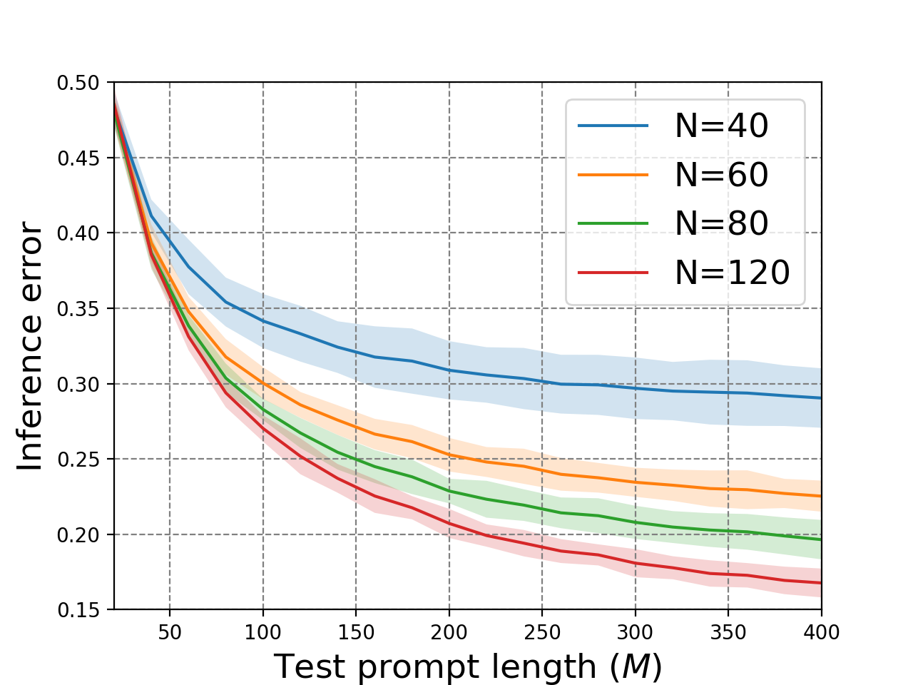
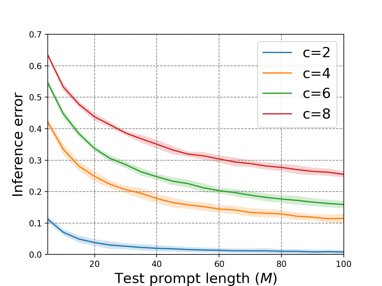
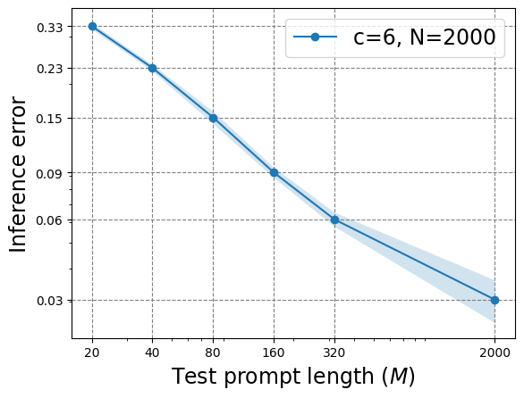
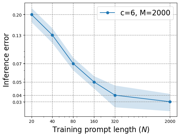
We first train single-layer transformers for in-context classification of Gaussian mixtures with different numbers of classes , different lengths of training prompts , and test them with different test prompt lengths . The results are reported in Figure 1. We can see from Figure 1 (a,b) that the inference errors decrease as and increase, and they increase as increases. In Figure 1 (c,d), we first fix the training prompt length (test prompt length) to a large number , and then vary the test prompt length (training prompt length) from 20 to 2000. The results show that, as and become sufficiently large, the inference error, which is an approximation of (see Appendix H for detailed definitions), decreases to near-zero. This indicates that the prediction of the trained transformer approaches the Bayes-optimal classifier. All these experimental results corroborate our theoretical claims.
5.2 Comparison of transformers with other machine learning algorithms
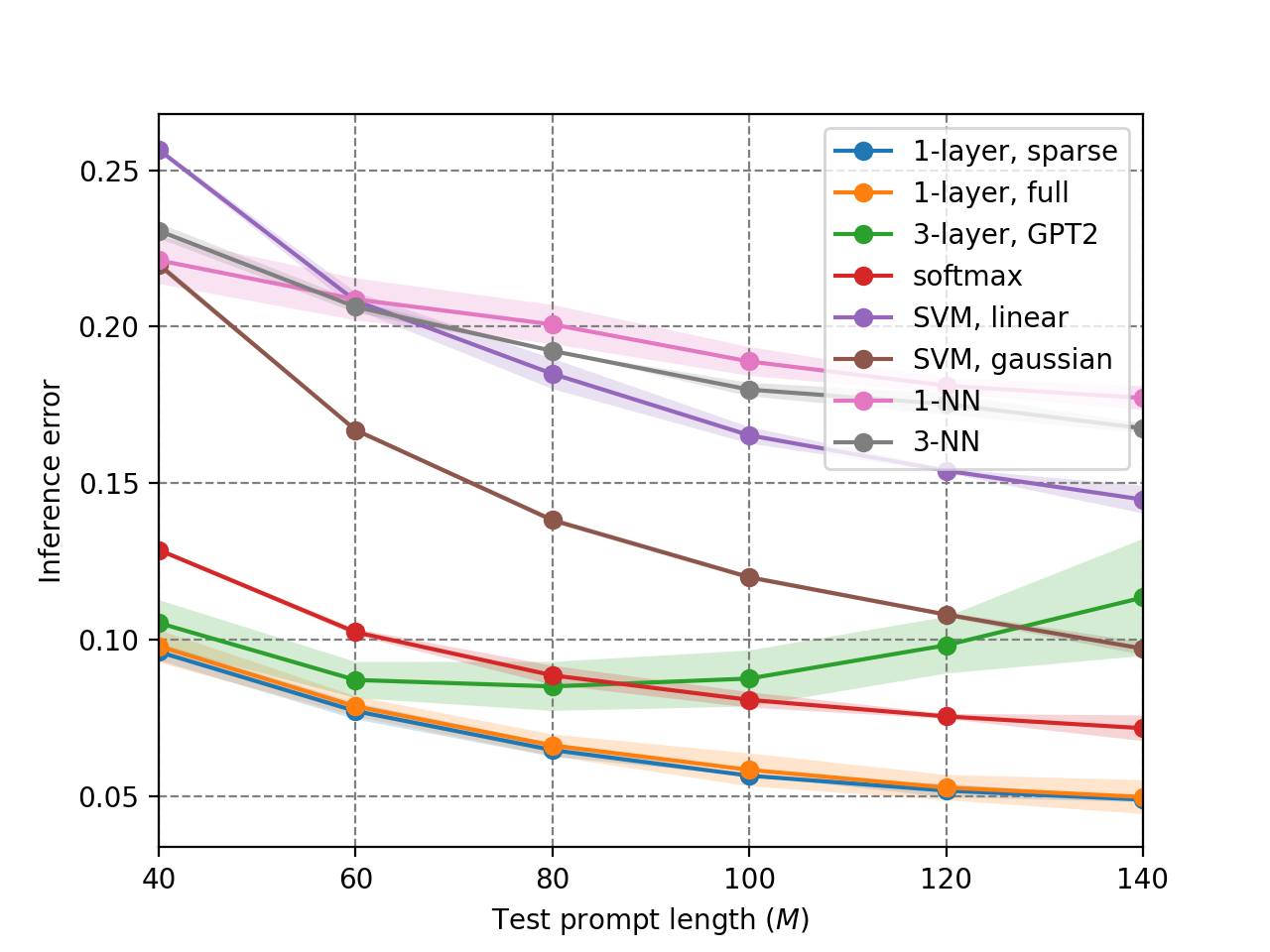
Additionally, we conduct experiments comparing the ICL performances of the transformers with other machine learning algorithms for the classification of three Gaussian mixtures. Again, the detailed experimental setting can be found in Appendix H. Form Figure 2, we can see that, when the prompt length is less than 100, all three transformer models have comparable or better performances than the traditional methods (softmax regression, SVM, -nearest neighbor), which demonstrates the strong ICL capacities of transformers. When the prompt length is larger than 100, a 3-layer transformer with the GPT-2 architecture shows a decline in performance, probably because our transformer models were only trained with a small prompt length of . Similar declined performance when the training prompt length is smaller than the test prompt length has also been observed for in-context linear regression tasks; see e.g. Zhang et al. (2023a). However, even when the prompt length is larger than 100, the single-layer transformer defined in Section 4 (1-layer, sparse) and the single-layer transformer with full parameters (59) (1-layer, full) still significantly outperform the traditional methods. This also indicates that, though the model (1-layer, sparse) we studied in this paper is relatively simple, this model is already sufficiently complex for in-context classification of Gaussian mixtures, both in theory and practice.
6 Conclusion
We studied the learning dynamics of transformers for in-context classification of Gaussian mixtures, and showed that with properly distributed data, a single-layer transformer trained via gradient descent converges to its global minimum. Moreover, we established the upper bounds of the inference errors of the trained transformers and discussed how the training and test prompt lengths influence the performance of the model. Experimental results also corroborated the theoretical claims. There are some directions worth further exploring. One potential avenue is to investigate whether the assumptions regrading the training and test prompts can be relaxed. Additionally, we have only examined single-layer transformers with linear attention and sparse parameters. The learning dynamics of multi-layer transformers with nonlinear attention (e.g., softmax) for in-context classification problems remain an interesting area for future investigation.
References
- Ahn et al. [2024] Kwangjun Ahn, Xiang Cheng, Hadi Daneshmand, and Suvrit Sra. Transformers learn to implement preconditioned gradient descent for in-context learning. Advances in Neural Information Processing Systems, 36, 2024.
- Akyürek et al. [2022] Ekin Akyürek, Dale Schuurmans, Jacob Andreas, Tengyu Ma, and Denny Zhou. What learning algorithm is in-context learning? investigations with linear models. arXiv preprint arXiv:2211.15661, 2022.
- Bai et al. [2024] Yu Bai, Fan Chen, Huan Wang, Caiming Xiong, and Song Mei. Transformers as statisticians: Provable in-context learning with in-context algorithm selection. Advances in neural information processing systems, 36, 2024.
- Brown et al. [2020] Tom Brown, Benjamin Mann, Nick Ryder, Melanie Subbiah, Jared D Kaplan, Prafulla Dhariwal, Arvind Neelakantan, Pranav Shyam, Girish Sastry, Amanda Askell, et al. Language models are few-shot learners. Advances in neural information processing systems, 33:1877–1901, 2020.
- Bubeck [2015] Sébastien Bubeck. Convex optimization: Algorithms and complexity, 2015.
- Chen et al. [2024] Siyu Chen, Heejune Sheen, Tianhao Wang, and Zhuoran Yang. Training dynamics of multi-head softmax attention for in-context learning: Emergence, convergence, and optimality. arXiv preprint arXiv:2402.19442, 2024.
- Cheng et al. [2023] Xiang Cheng, Yuxin Chen, and Suvrit Sra. Transformers implement functional gradient descent to learn non-linear functions in context. arXiv preprint arXiv:2312.06528, 2023.
- Dasgupta et al. [2022] Ishita Dasgupta, Andrew K Lampinen, Stephanie CY Chan, Antonia Creswell, Dharshan Kumaran, James L McClelland, and Felix Hill. Language models show human-like content effects on reasoning. arXiv preprint arXiv:2207.07051, 2022.
- Fu et al. [2023] Deqing Fu, Tian-Qi Chen, Robin Jia, and Vatsal Sharan. Transformers learn higher-order optimization methods for in-context learning: A study with linear models. arXiv preprint arXiv:2310.17086, 2023.
- Garg et al. [2022] Shivam Garg, Dimitris Tsipras, Percy S Liang, and Gregory Valiant. What can transformers learn in-context? a case study of simple function classes. Advances in Neural Information Processing Systems, 35:30583–30598, 2022.
- Giannou et al. [2023] Angeliki Giannou, Shashank Rajput, Jy-yong Sohn, Kangwook Lee, Jason D Lee, and Dimitris Papailiopoulos. Looped transformers as programmable computers. In International Conference on Machine Learning, pages 11398–11442. PMLR, 2023.
- Giannou et al. [2024] Angeliki Giannou, Liu Yang, Tianhao Wang, Dimitris Papailiopoulos, and Jason D Lee. How well can transformers emulate in-context newton’s method? arXiv preprint arXiv:2403.03183, 2024.
- Guo et al. [2023] Tianyu Guo, Wei Hu, Song Mei, Huan Wang, Caiming Xiong, Silvio Savarese, and Yu Bai. How do transformers learn in-context beyond simple functions? a case study on learning with representations. arXiv preprint arXiv:2310.10616, 2023.
- Huang et al. [2023] Yu Huang, Yuan Cheng, and Yingbin Liang. In-context convergence of transformers. arXiv preprint arXiv:2310.05249, 2023.
- Karimi et al. [2016] Hamed Karimi, Julie Nutini, and Mark Schmidt. Linear convergence of gradient and proximal-gradient methods under the polyak-łojasiewicz condition. In Machine Learning and Knowledge Discovery in Databases: European Conference, ECML PKDD 2016, Riva del Garda, Italy, September 19-23, 2016, Proceedings, Part I 16, pages 795–811. Springer, 2016.
- Kim and Suzuki [2024] Juno Kim and Taiji Suzuki. Transformers learn nonlinear features in context: Nonconvex mean-field dynamics on the attention landscape. arXiv preprint arXiv:2402.01258, 2024.
- Li et al. [2024] Hongkang Li, Meng Wang, Songtao Lu, Xiaodong Cui, and Pin-Yu Chen. Training nonlinear transformers for efficient in-context learning: A theoretical learning and generalization analysis. arXiv preprint arXiv:2402.15607, 2024.
- Li et al. [2023a] Yingcong Li, Muhammed Emrullah Ildiz, Dimitris Papailiopoulos, and Samet Oymak. Transformers as algorithms: Generalization and stability in in-context learning. In International Conference on Machine Learning, pages 19565–19594. PMLR, 2023a.
- Li et al. [2023b] Yuchen Li, Yuanzhi Li, and Andrej Risteski. How do transformers learn topic structure: Towards a mechanistic understanding. In International Conference on Machine Learning, pages 19689–19729. PMLR, 2023b.
- Lin et al. [2023] Licong Lin, Yu Bai, and Song Mei. Transformers as decision makers: Provable in-context reinforcement learning via supervised pretraining. arXiv preprint arXiv:2310.08566, 2023.
- Mahankali et al. [2023] Arvind Mahankali, Tatsunori B Hashimoto, and Tengyu Ma. One step of gradient descent is provably the optimal in-context learner with one layer of linear self-attention. arXiv preprint arXiv:2307.03576, 2023.
- Nichani et al. [2024] Eshaan Nichani, Alex Damian, and Jason D Lee. How transformers learn causal structure with gradient descent. arXiv preprint arXiv:2402.14735, 2024.
- Nye et al. [2021] Maxwell Nye, Anders Johan Andreassen, Guy Gur-Ari, Henryk Michalewski, Jacob Austin, David Bieber, David Dohan, Aitor Lewkowycz, Maarten Bosma, David Luan, et al. Show your work: Scratchpads for intermediate computation with language models. arXiv preprint arXiv:2112.00114, 2021.
- OpenAI [2023] OpenAI. GPT-4 technical report, 2023.
- Pathak et al. [2023] Reese Pathak, Rajat Sen, Weihao Kong, and Abhimanyu Das. Transformers can optimally learn regression mixture models. arXiv preprint arXiv:2311.08362, 2023.
- Radford [2018] Alec Radford. Improving language understanding by generative pre-training. 2018.
- Tarzanagh et al. [2023] Davoud Ataee Tarzanagh, Yingcong Li, Christos Thrampoulidis, and Samet Oymak. Transformers as support vector machines. arXiv preprint arXiv:2308.16898, 2023.
- Touvron et al. [2023] Hugo Touvron, Louis Martin, Kevin Stone, Peter Albert, Amjad Almahairi, Yasmine Babaei, Nikolay Bashlykov, Soumya Batra, Prajjwal Bhargava, Shruti Bhosale, et al. Llama 2: Open foundation and fine-tuned chat models. arXiv preprint arXiv:2307.09288, 2023.
- Vaswani et al. [2017] Ashish Vaswani, Noam Shazeer, Niki Parmar, Jakob Uszkoreit, Llion Jones, Aidan N Gomez, Łukasz Kaiser, and Illia Polosukhin. Attention is all you need. Advances in neural information processing systems, 30, 2017.
- Von Oswald et al. [2023] Johannes Von Oswald, Eyvind Niklasson, Ettore Randazzo, João Sacramento, Alexander Mordvintsev, Andrey Zhmoginov, and Max Vladymyrov. Transformers learn in-context by gradient descent. In International Conference on Machine Learning, pages 35151–35174. PMLR, 2023.
- Wang et al. [2023] Xinyi Wang, Wanrong Zhu, Michael Saxon, Mark Steyvers, and William Yang Wang. Large language models are implicitly topic models: Explaining and finding good demonstrations for in-context learning. In Workshop on Efficient Systems for Foundation Models@ ICML2023, 2023.
- Wei et al. [2022] Jason Wei, Yi Tay, Rishi Bommasani, Colin Raffel, Barret Zoph, Sebastian Borgeaud, Dani Yogatama, Maarten Bosma, Denny Zhou, Donald Metzler, et al. Emergent abilities of large language models. arXiv preprint arXiv:2206.07682, 2022.
- Wolf et al. [2020] Thomas Wolf, Lysandre Debut, Victor Sanh, Julien Chaumond, Clement Delangue, Anthony Moi, Pierric Cistac, Tim Rault, Rémi Louf, Morgan Funtowicz, et al. Transformers: State-of-the-art natural language processing. In Proceedings of the 2020 conference on empirical methods in natural language processing: system demonstrations, pages 38–45, 2020.
- Wu et al. [2023] Jingfeng Wu, Difan Zou, Zixiang Chen, Vladimir Braverman, Quanquan Gu, and Peter L Bartlett. How many pretraining tasks are needed for in-context learning of linear regression? arXiv preprint arXiv:2310.08391, 2023.
- Xie et al. [2021] Sang Michael Xie, Aditi Raghunathan, Percy Liang, and Tengyu Ma. An explanation of in-context learning as implicit bayesian inference. arXiv preprint arXiv:2111.02080, 2021.
- Yang et al. [2024] Tong Yang, Yu Huang, Yingbin Liang, and Yuejie Chi. In-context learning with representations: Contextual generalization of trained transformers. arXiv preprint arXiv:2408.10147, 2024.
- Zhang et al. [2023a] Ruiqi Zhang, Spencer Frei, and Peter L Bartlett. Trained transformers learn linear models in-context. arXiv preprint arXiv:2306.09927, 2023a.
- Zhang et al. [2024] Ruiqi Zhang, Jingfeng Wu, and Peter L Bartlett. In-context learning of a linear transformer block: benefits of the mlp component and one-step gd initialization. arXiv preprint arXiv:2402.14951, 2024.
- Zhang et al. [2022] Susan Zhang, Stephen Roller, Naman Goyal, Mikel Artetxe, Moya Chen, Shuohui Chen, Christopher Dewan, Mona Diab, Xian Li, Xi Victoria Lin, et al. Opt: Open pre-trained transformer language models. arXiv preprint arXiv:2205.01068, 2022.
- Zhang et al. [2023b] Yufeng Zhang, Fengzhuo Zhang, Zhuoran Yang, and Zhaoran Wang. What and how does in-context learning learn? bayesian model averaging, parameterization, and generalization. arXiv preprint arXiv:2305.19420, 2023b.
Appendix
The Appendix is organized as follows. In Section A, we provide a literature review of the related works that studied the ICL abilities of transformers. In Section B, we introduce the additional notations for the proofs in the Appendix. In Section C, we introduce some useful Lemmas we adopt from previous literature. In Sections D, E, F, G, we present the proofs of Theorem 3.1, 3.2, 4.1, 4.2 respectively. In Section H, we provide additional details of our experiments.
Appendix A Related work
It has been observed that transformer-based models have impressive ICL abilities in natural language processing [Brown et al., 2020, Nye et al., 2021, Wei et al., 2022, Dasgupta et al., 2022, Zhang et al., 2022]. Garg et al. [2022] first initiated the study of the ICL abilities of transformers in a mathematical framework and they empirically showed that transformers can in-context learn linear regression, two-layer ReLU networks, and decision trees. Subsequently, numerous works have been developed to explain the ICL capacities of transformers in solving in-context mathematical problems. These works mainly use two approaches: constructing specific transformers capable of performing certain in-context learning tasks, and studying the training dynamics of transformers for such tasks.
Constructions of transformers. Akyürek et al. [2022], Von Oswald et al. [2023] showed by construction that multi-layer transformers can be viewed as multiple steps of gradient descent for linear regression. Akyürek et al. [2022] also showed that constructed transformers can implement closed-form ridge regression. Guo et al. [2023] showed that constructed transformers can perform in-context learning with representations. Bai et al. [2024] proved that constructed transformers can perform various statistical machine learning algorithms through in-context gradient descent and showed that constructed transformers can perform in-context model selection. Lin et al. [2023] demonstrated that constructed transformers can approximate several in-context reinforcement learning algorithms. Fu et al. [2023], Giannou et al. [2024] further proved that constructed transformers can perform higher-order optimization algorithms like Newton’s method. Pathak et al. [2023] showed that transformers can learn mixtures of linear regressions. Giannou et al. [2023] proved that looped transformers that can emulate various in-context learning algorithms. Cheng et al. [2023] showed that transformers can perform functional gradient descent for learning non-linear functions in context. Zhang et al. [2024] showed that a linear attention layer followed by a linear layer can learn and encode a mean signal vector for in-context linear regression.
Training dynamics of transformers. Mahankali et al. [2023], Ahn et al. [2024] proved that the global minimizer of the in-context learning loss of linear transformer can be equivalently viewed as one-step preconditioned gradient descent for linear regression. Zhang et al. [2023a] proved the convergence of gradient flow on a single-layer linear transformer and discussed how training and test prompt length will influence the prediction error of transformers for linear regression. Huang et al. [2023] proved the convergence of gradient descent on a single-layer transformer with softmax attention with certain orthogonality assumptions on the data features. Li et al. [2023b] showed that trained transformers can learn topic structure. Wu et al. [2023] analyzed the task complexity bound for pretraining single-layer linear transformers on in-context linear regression tasks. Tarzanagh et al. [2023] built the connections between single-layer transformers and support vector machines (SVMs). Nichani et al. [2024] showed that transformers trained via gradient descent can learn causal structure. Chen et al. [2024] proved the convergence of gradient flow on a multi-head softmax attention model for in-context multi-task linear regression. Kim and Suzuki [2024], Yang et al. [2024] proved that trained transformers can learn nonlinear features in context.
Recently, Li et al. [2024] studied the training dynamics of a single layer transformer for in-context classification problems. However, they only studied the binary classification tasks with finite patterns. They generated their data as , where are in-domain-relevant patterns and are in-domain-irrelevant patterns, and these patterns are all pairwise orthogonal. Thus, the possible distribution of their data is finite and highly limited. In contrast, our work explores the ICL capabilities of transformers for both binary and multi-class classification of Gaussian mixtures. Specifically, our data is drawn according to or , and the range and possible distributions of our data are infinite. Furthermore, the transformer architectures analyzed in their work also differ from those in our study, thereby highlighting the distinct contributions and independent interests of our work.
Some works also studied the ICL from other perspectives. To name a few, Xie et al. [2021] explained the ICL as implicit Bayesian inference; Wang et al. [2023] explained the LLMs as latent variable models; Zhang et al. [2023b] explained the ICL abilities of transformers as implicitly implementing a Bayesian model averaging algorithm; and Li et al. [2023a] studied the generalization and stability of the ICL abilities of transformers.
Appendix B Additional notations
We denote if a random variable follows the binomial distribution with parameters and , which means . We denote if random variables follow the Multinomial distribution with parameters and , which means . We denote for simplicity. We define , . For , we define .
Appendix C Useful lemmas
Lemma C.1 ([Karimi et al., 2016])
If is -strongly convex, then
where .
Lemma C.2 ([Bubeck, 2015])
Suppose is -strongly convex and -smooth for some . Then, the gradient descent iterating with learning rate and initialization satisfies that for any ,
where is the condition number of , and is the minimizer of .
Appendix D Training procedure for in-context binary classification
In this section, we present the proof of Theorem 3.1.
D.1 Proof sketch
First, we prove in Lemma D.2 that the expected loss function in (7) is strictly convex w.r.t. and is strongly convex in a compact set of . Moreover, we prove has one unique global minimizer . Then, in Lemma D.3, by analyzing the Taylor expansion of , we prove that as , our loss function point wisely converges to (defined in (25)), and the global minimizer converge to . We denote , and prove . Next, in Lemma D.4, by further analyzing the Taylor expansion of the equation at the point , we establish a tighter bound . In Lemma D.5, we prove that our loss function is -smooth and provide an upper bound for . Thus, in a compact set , our loss function is -strongly convex and -smooth. Finally, leveraging the standard results from convex optimization, we prove Theorem 3.1 in subsection D.4.
In this section, we use the following notations.
D.2 Notations
Recall the expected loss function (7) is
| (21) |
where
is the output of the transformer, and the label of the data follows the distribution
In this section, we introduce the following notations to analyze (7). We denote , , and . Then with probability we have , and with probability we have , where . We define . Since with probability we have , and with probability we have , where , we known , where , , . Defining , , we have and
| (22) |
Then, the expected loss function (7) can be expressed as
| (23) |
The gradient of the loss function (7) can be expressed as
| (24) |
Moreover, we define a function as
| (25) |
In Lemma D.3, we show that as , will point wisely converge to .
D.3 Lemmas
Lemma D.1
Suppose . Defining , we have
Proof Since , the moment-generating function of is
We can compute the moment-generating function of as follows:
Thus, we know the coefficients of , , are respectively, and the coefficients of are . We have
Moreover, according to the Jensen’s inequality, we have
Lemma D.2
For the loss function (7), we have . For any compact set of , when , we have for some . Additionally, has one unique global minimizer on .
For defined in (25), we also have . For any compact set of , when , we have for some . Additionally, has one unique global minimizer on .
Considering such that , we have
where are the probability density function (PDF) function of . Since for any , , we have . Thus, and is convex.
Moreover, for any , we denote . Suppose , we consider a set of constants , where , , and , . Then, for any . We have
Then, we define region , ,. We have
Defining
we have . Since with probability , , with probability , , where and , where , the covariance matrices of are positive definite and we have for all . Moreover, are non-zero measures on . Thus, we have . Then, for any , we have
Thus, we have . is strictly convex.
Moreover, for any compact set of , for any , we have
Then, for any , for any , we have
Thus, when , where is a compact set, we have and the loss function is strongly convex, where .
Because our loss function is strictly convex in , it has at most one global minimizer in . Next, we prove all level sets of our loss function are compact, i.e. is compact for all . We prove it by contradiction. Suppose is not compact for some . Since our loss function is continuous and convex, is an unbounded convex set. Since the dimension of is , consider a point , there must exists a such that . For this , there must exist a set of constants such that for any , we have
Thus, we have
We define , , . Then, defining
we have . Since are non-zero measures for , we have . Then, we have
This contradicts the assumption . Thus, all level sets of the loss function are compact, which means there exists a global minimizer for . Together with the fact that is strictly convex, has one unique global minimizer on .
Similarly, we can prove the same conclusions for .
Lemma D.3
Denoting the global minimizer of the loss function (7) as , we have , where .
Proof Let , , . Performing the Taylor expansion on (7), we have
where are real numbers between and . According to Lemma D.1, we have . Thus, we have
Moreover, we have
where is due to Lemma D.1, and . is a constant independent of and . Thus, we have
This shows that point wisely converges to .
According to Lemma D.2, has one unique global minimizer. Consider the equation:
We can easily find that and is the global minimizer of .
Considering a compact set , we have for . Here are some positive finite constants. Then, we have
where is a constant independent of and . This shows that, for , our loss function uniformly converge to .
Denote as the global minimizer of the loss function with prompt length . Then, we show that, when is sufficiently large, . We first denote and . Then, for , and for any , we have
This means
Since is strictly convex, we have .
Then, we have
and
According to Lemma D.2, for , we have , where is a positive constant independent of . Thus, is -strongly convex in . According to Lemma C.1, we have
Thus, when , we have . Denoting , we have .
Lemma D.4
Proof According to Lemma D.2, the loss function has a unique global minimizer . We have
| (27) |
Let , , . We have
The Taylor expansion of at point with an Lagrange form of remainder is
where are real numbers between and . Thus, our equation (27) become
| (28) |
Note that . For , according to Lemma D.1 and , we have
| (29) |
Then, we have
where is a constant independent of . According to Lemma D.3, , we have
| (30) |
Similarly for , we have
Each term in contains two ’s. Thus, their max norms are at most . For each term in , it contains one and or contains one and two . According to in Lemma D.1, the max norm of terms with one and are smaller than . Defining , we have and . Thus, converting two to , we have a coefficient of . Therefore, the max norms of terms with one and two are also smaller than . Therefore, for terms , we have
| (31) | |||
| (32) |
For term , according to Lemma D.1 and , we have
| (33) | ||||
| (34) |
For , we have
For terms in containing two or three , these terms’ expected absolute values are at most smaller than . For terms in containing one , these terms must contain number of and number of elements of , where . According to Lemma D.1, we know that for , . Defining , we have and . Converting to , we have a coefficient of . Thus, for terms in , these terms’ expected absolute values are at most smaller than . For terms in without , these terms must contain number of and number of elements of , we have . Similarly, these term’s expected absolute values are at most smaller than . Therefore, we have
| (35) |
Moreover, we have
| (36) |
where . We vectorize as . Define , where . Then (36) can be expressed as
| (37) |
Note that . According to Lemma D.2, is positive definite. Thus, combining (28), (29), (30), (31), (32), (34), (35), (37), we have
Lemma D.5
The loss function (7) is -smooth, where .
Proof The Hessian matrix of the loss function is
Considering such that , we have
where is due to the Cauchy–Schwarz inequality. Thus, and is -smooth, where is a constant smaller than .
D.4 Proof of Theorem 3.1
Proof According to Lemma D.4, the global minimizer of is , where
| (38) |
Define . is a compact set. Then, according to Lemma D.2, for , we have . Here is a positive constant number. Thus, is -strongly convex in . Moreover, according to Lemma D.5, is -smooth. Then according to Lemma C.2, applying gradient descent with , for any , we have
where .
Appendix E In-context inference of binary classification
E.1 Notations
In this section, we use the following notations. We denote , , . Define . Since with probability , , with probability , , where , we have , where , , . Defining , , we have and
| (39) |
E.2 Proof of Theorem 3.2
Proof The output of the trained transformer is
| (40) |
The probability of given is
Defining , , we have
and
where are real numbers between and . Thus, we have
We first consider the term . Defining , we have
where is due to in Lemma D.1. is because that and , for .
For , we have
Notice that terms in contain two . Thus, they are at most smaller than . Terms in contain two , or two , or one and one . According to Lemma D.1, we have , . Moreover, . Converting one to , we have a coefficient of . Thus, terms in contain two , or two , or one and one are . Terms in contain at least one and one or one and one . Thus, they are at most smaller than . Therefore, we have .
Finally, we have
Remark E.1
We note that Theorem 3.2 requires Assumption 3.2 to hold. For example, we need the covariance in training and testing to be the same. A similar consistency requirement of the covariance in training and testing had also been observed for in-context linear regression in Zhang et al. [2023a].
Here, we discuss the consequences when Assumption 3.2 does not hold. For example, suppose the labels of our data in test prompts are not balanced where . Besides, do not have the same weighted norm, and the covariance matrix of test data is . Then, as , we have
and
On the other hand, the distribution of the ground truth label is
Define and . Then, we can notice that unless or is sufficiently small, the transformer cannot correctly perform the in-context binary classification.
Appendix F Training procedure for in-context multi-class classification
In this section, we present the proof of Theorem 4.1.
F.1 Proof sketch
First, we prove in Lemma F.3 that the expected loss function (16) is strictly convex w.r.t. and is strongly convex in a compact set of . Moreover, we prove has one unique global minimizer . Then, in Lemma F.4, by analyzing the Taylor expansion of , we prove that as , our loss function point wisely converges to (defined in (44)), and the global minimizer converge to . Thus, we denote , and prove . Next, in Lemma F.5, by further analyzing the Taylor expansion of the equation at the point , we establish a tighter bound . In Lemma F.6, we prove that our loss function is -smooth and provide an upper bound for . Thus, in a compact set , our loss function is -strongly convex and -smooth. Finally, leveraging the standard results from the convex optimization, we prove Theorem 4.1 in subsection F.3.
In this section, we use the following notations.
F.2 Notations
Recall the expected loss function (16) is
| (41) |
where
is the output of the transformer, and the label of the data follows the distribution
In this section, we introduce the following notations to analyze (16). We denote , and . Then with probability , , where . We define and . We have . Since with probability we have , where , we known , where , and . Defining , we have and . Defining , we have . Defining and , we have .
Then, the expected loss function (16) can be expressed as
| (42) |
The gradient of the loss function (16) can be expressed as
| (43) |
Moreover, we define a function as
| (44) |
In Lemma F.4, we show that as , will point wisely converge to .
Lemma F.1
Suppose . Defining , we have
where .
Proof Since , the moment-generating function of is
We can compute the moment-generating function of as follows:
Observing the coefficients of , we have
where .
Iteratively applying the Hölder’s inequality, we have
where .
Lemma F.2
Suppose and , define and , we have
where .
For any , satisfying , we have
Moreover, we have
where .
For any , satisfying , , we have
Proof Since and , we have
where . Thus, with the results from Lemma F.1, for any , satisfying , we have
Moreover, according to the Jensen’s inequality, we have
where . Thus, with the results from Lemma F.1, for any , satisfying , , we have
Lemma F.3
For the loss function (16), we have . For any compact set , when , we have for some . Additionally, has one unique global minimizer on .
For defined in (44), we also have . For any compact set , when , we have for some . Additionally, has one unique global minimizer on .
Proof We vectorize as , where , . Then, we have
| (45) |
Note that
where . For , we have
Then we have
and
We can express the Hessian matrix of the loss function with the following form:
Considering such that , we have
Since for any , , , we have . Thus, and is convex.
Defining , we have
where are the PDF function of . For any , we denote , suppose , we consider a set of constants , where , , and , . Then, for any , we have
Then, we define region , ,. We have
Defining
we have . Since we have for all and are non-zero measures for . Thus, we have . Then, for any , we have
Thus, we have . is strictly convex.
Moreover, for any compact set of , for any , we have
Then, for any , for any , we have
Thus, when , is a compact set, we have , our loss function is strongly convex, where .
Because our loss function is strictly convex in , it has at most one global minimizer in . Next, we prove all level sets of our loss function are compact, i.e. is compact for all . We prove it by contradiction. Suppose is not compact for some . Since our loss function is continuous and convex, is an unbounded convex set. Since the dimension of is , consider a point , there must exists a that . For this , there must exist a set of constants such that for any , we have
Thus, we have
We define , , . Then, defining
we have . Since are non-zero measures for , we have . Then, we have
This contradicts the assumption . Thus, all level sets of the loss function are compact, which means there exists a a global minimizer for . Together with the fact that is strictly convex, has one unique a global minimizer on .
Similarly, we can prove the same conclusions for .
Lemma F.4
Denoting the global minimizer of our loss function (16) as , we have , where .
Proof Let , , , , , . Performing the Taylor expansion on (16), we have
where . Thus, we have
where the last inequality is due to Lemma F.1, F.2. is a constant independent of and . This shows that point wisely converge to .
According to Lemma D.2, has one unique global minimizer. Considering the equation:
We can easily find that and is the global minimizer of .
Considering a compact set , we have for any . Here are some positive finite constants. Then, we have
where is a constant independent of and . This shows that, for any , uniformly converge to .
Denote as the global minimizer of with prompt length . Then, we show that, when is sufficiently large, . We first denote , . Then, for , and for any , we have
Since is strictly convex, we have .
Then, we have
According to Lemma D.2, for , we have , where is a positive constant independent of . Thus, is -strongly convex in . According to Lemma C.1, we have
Thus, when , we have . Denoting , we have .
Lemma F.5
The global minimizer of the loss function (16) is . We have
where , , . Ignoring constants other than , we have .
Proof According to Lemma F.3, the loss function has a unique global minimizer . We have
| (46) |
For the second term , we have
For terms having two , their max norms are at most smaller than . For terms having one , define , these terms must contain number of and number of , we have . According to Lemma F.2, we know that for ,
Thus, the max norm of expectations of terms in (ii) are at most smaller than . Therefore, for terms , we have
| (50) | |||
| (51) |
For terms without , we have
| (52) |
For the third term , we have
For terms in having two or three , these terms’ expected absolute values are at most smaller than . For terms in having one , these terms must contain number of and number of , we have . According to Lemma F.2, for , we have
Thus, these term’s expected absolute values are at most smaller than . For terms in without , these terms must contain number of and number of , we have . According to Lemma F.2, for , we have
Thus, these term’s expected absolute values are at most smaller than . Therefore, we have
| (53) |
Moreover, we have
| (54) |
where . We vectorize as . Define , where , (54) can be expressed as
| (55) |
Note that . According to Lemma F.3, is positive definite. Thus, combining (47), (48), (49), (50), (51), (52), (53), (55), we have
Ignoring constants other than , we have .
Lemma F.6
The loss function (7) is -smooth, where .
Proof The Hessian matrix of the loss function is
Considering such that , we have
where is due to the Cauchy–Schwarz inequality. Thus, and is -smooth, where is a constant smaller than .
Theorem F.1 (Formal statement of Theorem 4.1)
The following statements hold.
-
(1)
Optimizing training loss (16) with training prompt length via gradient descent , we have for any
where is the initial parameter and is the global minimizer of , . are constants such that
(56) where .
-
(2)
Denoting , we have
where , . The expectation is taken over , .
-
(3)
After gradient steps, denoting as the final model, we have
(57) where .
F.3 Proof of Theorem 4.1
Proof According to Lemma F.5, the global minimizer of is , where
Ignoring constants other than , we have .
Define , and is a compact set. Then, according to Lemma F.3, for , we have . Here is a positive constant number. Thus, is -strongly convex in . Moreover, according to Lemma F.6, is -smooth. Then according to Lemma C.2, applying gradient descent with , for any , we have
where .
After gradient steps, we have , where , . Thus, .
Appendix G In-context inference of multi-class classification
G.1 Notations
In this section, we use the following notations. We denote , . Define , and define . We have . Since with probability , , where , we have , where , and . Defining , we have and .
G.2 Proof of Theorem 4.2
Proof The output of the trained transformer is
| (58) |
The probability of given is
Defining , , , , we have
where . Thus, we have
We first consider the term . Defining , we have
where is due to Lemma F.1 that . is because that , , for .
For , we have
For terms having two , they are at most smaller than . For terms having one , these terms must contain number of and number of , we have . According to Lemma F.2, we know that for ,
Thus, terms in (ii) are at most smaller than . For terms without , these terms must contain number of and number of , we have . According to Lemma F.2, for , we have
Thus, these term are . Therefore, we have .
Finally, we have
Remark G.1
We note that Theorem 4.2 requires Assumption 4.2 to hold. For example, we need the covariance in training and testing to be the same. A similar consistency requirement of the covariance in training and testing had also been observed for in-context linear regression in Zhang et al. [2023a] and for in-context binary classification in the previous section 3.2.
Here, we discuss the consequences when Assumption 4.2 does not hold. For example, suppose the labels of our data in test prompts are not balanced , do not have the same weighted norm , and the covariance matrix of test data is , then as , we have
and
Denote , and . Then distribution of the ground truth label is
Define . Then, unless or is sufficiently small, the transformer cannot correctly perform the in-context multi-class classification.
Appendix H Experiment details
For all tasks, we set and we randomly generate a covariance matrix , where and . For each training dataset with different training prompt lengths , and different class numbers , we randomly generate training samples. Training prompts and their corresponding labels are generated according to Assumption 4.1. Moreover, we also generate testing datasets. For example, for each testing dataset, we first randomly generate 20 pairs of , where , . are the corresponding probability distributions of the ground truth label . For each , we generate 100 testing prompts , where . We denote a model’s output for testing prompts as . We calculate its inference error with , which serves an approximation of the expected total variation distance we defined in (3).
For experiments in Figure 1, we train the single-layer transformers with the sparse-form parameters and structures defined in Section 4. We set the size of the training dataset to and set the batch size to 50. We train the transformers using SGD with learning rate for 10 epochs, and get the best model on each training dataset. Then, we test these trained models on different testing datasets. Each experiment is repeated 10 times with different random seeds. The mean results and standard deviation error bars of these 10 experiments are plotted in Figure 1.
For experiments in Figure 2, the structure of the transformer with full parameters (1-layer, full) is defined as
| (59) |
where are the parameters for optimization. For the (3-layer, GPT2) model, we use the GPT2 architecture [Radford, 2018] with 64 embedding sizes, 3 layers and 2 heads as implemented by HuggingFace [Wolf et al., 2020], and we use the similar embedding method proposed by Garg et al. [2022]. Note that, for the GPT2 model trained on prompt length , it will produce predictions for the labels , . Assume the ground truth labels for the prompt is , , usually, for decoder models like GPT2, we should define the loss function as , which can be viewed to some extent as the model is trained with prompts length ranging from 0 to 100. However, for in-context classification of Gaussian mixtures, longer prompts are significantly more helpful for training models than shorter prompts. For example, considering an extreme case where the classification task involves classes and the training prompt length is smaller than , then it is nearly impossible for the model to learn to classify classes Gaussian mixtures in context with these short prompts. Our Theorems 3.1 and 4.1 also clearly demonstrate that the training error is inversely proportional to the prompt length with a scaling of . Thus, if we define the loss function for GPT2 as , the underlying short prompts will be detrimental to the model training. Therefore, in our experiments, we define the loss function for our GPT2 model as , which can be viewed to some extent as the model that is trained with prompts length ranging from 40 to 100. For all three transformer models, we set the size of the training dataset to and set the batch size to 50. We train the (1-layer, sparse) and (1-layer, full) using Adam with learning rate 0.001 for 5 epochs, and train the GPT2 model using Adam with learning rate 0.0001 for 5 epochs. Each experiment is repeated 3 times with different random seeds. The mean results and standard deviation error bars of these 3 experiments are plotted in Figure 2.