Time-Series Foundation Model for Value-at-Risk

Abstract

This study is the first to explore the application of a time-series foundation model for Value-at-Risk (VaR) estimation. Foundation models, pre-trained on vast and varied datasets, can be used in a zero-shot setting with relatively minimal data or further improved through finetuning. We compare the performance of Google’s model, called TimesFM, against conventional parametric and non-parametric models, including GARCH, Generalized Autoregressive Score (GAS), and empirical quantile estimates, using daily returns from the S&P 100 index and its constituents over 19 years. Our backtesting results indicate that in terms of the actual-over-expected ratio the fine-tuned TimesFM model consistently outperforms traditional methods. Regarding the quantile score loss function, it achieves performance comparable to the best econometric approach, the GAS model. Overall, the foundation model is either the best or among the top performers in forecasting VaR across the 0.01, 0.025, 0.05, and 0.1 VaR levels. We also found that fine-tuning significantly improves the results, and the model should not be used in zero-shot settings.

[inst1]organization=Tampere University, Department of Computing Sciences, Financial Computing and Data Analytics Group,addressline=Kalevantie 4, city=Tampere, postcode=33100, country=Finland

[inst2]organization=IIT Ropar, Department of Mathematics,addressline=Ropar, city=Punjab, postcode=140001, country=India

1 Introduction

While the application of Machine Learning (ML) in various fields in financial market research has gained significant attention—such as in asset pricing, volatility forecasting, limit order book dynamics, and optimal hedging (Gu et al., 2020; Christensen et al., 2023; Tran et al., 2018; Mikkilä and Kanniainen, 2023)—the risk management literature still largely relies on traditional econometric techniques, especially in the area of Value-at-Risk (VaR). One reason for this may be that Deep Learning (DL) models require substantial amounts of data, which poses a significant limitation when applying them to calculate risk metrics for individual stocks. VaR estimations are often based on daily return observations (for example, see González-Rivera et al., 2004; Patton et al., 2019; Taylor, 2019, based solely on historical daily returns), and even 20 years of data would yield only around 5,000 observations. This is quite limited, especially considering that DL models often contain millions of parameters that need to be learned.

However, a solution to this problem is currently underway. Recently, machine learning has experienced a paradigm shift with the emergence of foundation models, which are large-scale, general-purpose pre-trained and often fine-tunable models on diverse datasets spanning various data distributions. Although foundation models are built on standard deep learning and transfer learning principles, their scale leads to the emergence of new capabilities (Bommasani et al., 2021). In 2023–2024, following major advancements in large language models (LLMs), several pre-trained time-series foundation models have emerged, including Google’s TimesFM (Das et al., 2024), Time-GPT (Garza and Mergenthaler-Canseco, 2024), and LagLlama (Rasul et al., 2023).

AI-driven advancements in financial risk modeling have opened doors to new methodologies for assessing complex financial data (Tran et al., 2019; Guijarro-Ordonez et al., 2021; Chen et al., 2024). Historically, methods like GARCH-based models have been effective for capturing dependencies and volatility clustering in market data Hoga and Demetrescu (2023). Recent approaches, however, such as Generative Adversarial Networks (GANs), Variational Autoencoders (VAEs), and Conditional GANs (CGANs), extend these capabilities by generating realistic synthetic data for distribution forecasting (Nareklishvili et al., 2023; Athey et al., 2021; Hofert et al., 2022). These generative models allow for flexible, non-parametric modeling of data structures that were once challenging to approximate with traditional econometric tools. Ericson et al. (2024) provide a comprehensive comparative review, highlighting that deep generative methods outperform traditional benchmarks in capturing complex financial dynamics for VaR estimation. These advancements underscore the potential of AI-driven methods in risk forecasting. Our approach diverges by utilizing a time-series foundation model, pre-trained on extensive and various data sets, to predict VaR. Compared to traditional supervised ML models, which are trained for specific tasks, these time-series forecasting models are pre-trained on vast, diverse datasets containing billions of real-world time points. A single pre-trained model can be applied across a wide range of domains, from traffic forecasting to stock price predictions, offering quick and cost-effective solutions. The word ‘foundational’ emphasizes their flexibility, as they can be adapted for different tasks or domains with minimal additional training. The foundation models can be used with or without fine-tuning.

We implement a pre-trained time-series foundation model, specifically Google’s TimesFM, for VaR estimation and compare it with existing state-of-the-art parametric and semi-parametric approaches, including GARCH model, Generalized Autoregressive Score (GAS) one-factor model, and empirical quantile estimates. The key question is whether the pre-trained foundation model yields results comparable to, or even capable of outperforming, existing econometric methods. Additionally, this paper seeks to determine how much fine-tuning enhances accuracy in the context of VaR predictions. This paper could employ alternative foundation models as several have been published recently, and more are on the way. However, we decided to focus on the use TimesFM because it is an open-source, modifiable, and free-of-charge, making our results completely replicable. Moreover, our goal is not to find the best possible foundation model among those available, as they are likely to be modified and entirely new ones can be published on a monthly basis, but rather to address more fundamental question if the state-of-the-art parametric and semi-parametric approaches can be outperformed.

We conduct an extensive empirical evaluation of the performance of the foundation time-series model with daily return data on the 91 constituents of the S&P 100 index over 19 years. For each constituent, we calculate 1-day VaR on a daily basis. The foundation model is applied both with and without fine-tuning to understand how much the results improve with fine-tuning, which has certain computational cost. The fine-tuning is performed on a daily basis using a rolling window technique.

Our main finding is that, in terms of the actual-over-expected ratio, the fine-tuned time-series foundation model outperforms existing econometric approaches for VaR estimation. Specifically, the fine-tuned foundation model consistently demonstrates superior performance, on average, across all 91 constituents of the S&P 100 included in the analysis. Regarding the quantile score loss function, which was the second backtesting metric, the fine-tuned foundation model achieves performance comparable to the best econometric approach, the GAS model. Overall, the foundation model is either the top performer or among the best in forecasting VaR across the 0.01, 0.025, 0.05, and 0.1 VaR levels. Moreover, we found that fine-tuning is practically necessary for the foundation model; using it as pre-trained in zero-shot settings results in clearly worse performance compared to the best econometric approaches. We consider this as a remarkable result on the performance of Google’s TimesFM model as this model is not explicitly designed for this purpose and was not even pre-trained with stock return data. This problem is statistically challenging due to its focus on heteroscedastic processes with time-varying conditional volatility. In this light, the paper is valuable not only for financial risk management but also as a benchmark to test AI time-series models against state-of-the-art statistical approaches on a highly complex issue.

The paper is structured as follows: In Section 2, we describe the time-series foundation model, Google’s TimesFM, and the benchmark models against which it is compared. Section 3 details the data and experimental setup for the models and fine-tuning specifications for VaR estimation. The evaluation metrics and backtesting procedures are outlined in Section 4. Section 5 presents an analysis of the empirical results, examining the performance of the foundation model relative to traditional econometric approaches. Finally, the findings have several implications beyond Value-at-Risk estimation techniques, which, along with the limitations of our analysis, will be discussed at the end of the paper in Section 6.

2 Models

2.1 Time-Series Foundation Models

The time-series foundation models share similarities with large language models (LLMs) as they rely on transformer-based architectures to capture long-range dependencies and patterns within sequential data. While LLMs are trained to predict the next or missing part of a text sequence, foundational time-series models process continuous time points as individual tokens. This approach allows them to handle time-series data step by step.

TimesFM model (Das et al., 2024) is a decoder-only transformer architecture, similar to GPT models. In contrast to encoder-decoder models, where the encoder processes the input sequence and the decoder generates output based on the encoded input, decoder-only models focuse solely on output generation processing the input through successive decoder layers. This allows for faster training and inference times compared to encoder-decoder models. Decoder-only models like are highly advantageous for zero-shot forecasting, where minimal fine-tuning is required. On the other hand, the advantage of the encoder-decoder architecture, which is used, for example, in TimeGPT (Garza and Mergenthaler-Canseco, 2024), is that it can handle more complex inputs and exogenous variables. However, in this paper, we use univariate and well-structured time-series data on returns, and VaR is calculated separately for each security, and for that reason the encoder component does not add significant value.

The architecture of TimesFM is optimized for long-horizon forecasting through the use of a patching strategy, where the time-series data is broken into patches. These patches function similarly to tokens in language models, significantly improving efficiency. Unlike some autoregressive models that predict one step at a time, TimesFM predicts longer output patches at once, reducing the number of necessary auto-regressive steps. This makes the model particularly well-suited for handling varying context lengths, prediction lengths, and temporal granularities during inference.

In pretraining, TimesFM was trained on a vast corpus comprising both real-world time-series data such as Google trends, Wiki Pageviews, Synthetic Data, and Electricity, Traffic, and Weather datasets used in M4 competition (Makridakis et al., 2020; Spiliotis et al., 2020). However, financial data was not used, and this aspect makes the application of the present paper particularly interesting. This corpus, although smaller in scale compared to text-based models, spans around 100 billion time points, providing the diversity needed for the model to generalize well across domains and forecasting tasks. Compared to the state-of-the-art LLMs, TimesFM time-series foundation model is much smaller, with 200M parameters and pretraining data consisting of around 100B timepoints. Despite its smaller scale, it was reported to achieve relatively high zero-shot forecasting accuracy

2.2 Benchmark Models for VaR

To evaluate the performance of the foundation time series models for estimating Value-at-Risk, we benchmark it against several established models. These include both traditional and advanced methods, each with its own set of assumptions and computational characteristics. The benchmark models are as follows:

• Rolling Window Quantile Estimation:

  One of the most widely used approaches for VaR estimation is the rolling window method, which computes the risk measure based on historical data over a fixed time window:

  $$\widehat{\text{VaR}}_{t}=\text{Quantile}\left\{r_{i}\right\}_{i=t-m}^{t-1},$$

  where $\text{Quantile}\left\{r_{i}\right\}_{i=t-m}^{t-1}$ represents the sample quantile of the variable $r_{i}$ over the period $i\in[t-m,t-1]$. The parameter $m$ denotes the size of the rolling window. While this approach is straightforward and easy to implement, it does not account for the dynamic nature of financial markets, leading to potential inaccuracies during periods of high volatility.

• ARMA-GARCH Models (Angelidis et al., 2004):

  To better capture the time-varying properties of financial returns, we employ ARMA-GARCH models. These models estimate the conditional mean and variance of returns, incorporating various distributional assumptions for the standardized residuals. The model is specified as

  $$r_{t}=\mu_{t}+\sigma_{t}\eta_{t},\text{\quad}\eta_{t}\sim\text{iid }\mathbb{G}_{\eta}(0,1).$$

  In this framework, $\mu_{t}$ represents the conditional mean, typically modeled using an ARMA process, while $\sigma_{t}^{2}$ denotes the conditional variance, modeled using a GARCH process. The standardized residuals $\eta_{t}$ follow a distribution $\mathbb{G}_{\eta}$ with mean zero and variance one. The VaR for these models is calculated as

  $$v_{t}=\mu_{t}+\sigma_{t}a_{\alpha},\quad\text{where }a_{\alpha}=\mathbb{G}_{\eta}^{-1}(\alpha).$$

  Here, $a_{\alpha}$ is the $\alpha$-quantile of the distribution $\mathbb{G}_{\eta}$. Different assumptions for $\mathbb{G}_{\eta}$ yield various model specifications, including:

  1. Normal GARCH: This specification assumes that the residuals follow a normal distribution:

     $$\eta_{t}\sim\text{iid }N(0,1).$$

     This is the most basic assumption and is often insufficient for capturing the heavy tails observed in financial return distributions.

  2. Student’s t-GARCH: To account for the heavy tails and potential skewness in the return distribution, a skewed t-distribution is used for the residuals:

     $$\eta_{t}\sim\text{iid Skew }t(0,1,\nu,\lambda).$$

     This model provides greater flexibility in capturing the tail behavior of financial returns, which is crucial for accurate risk estimation.

  3. Empirical Distribution Function: As a nonparametric alternative, we use the Empirical Distribution Function (EDF) method (Manganelli and Engle, 2004). This approach estimates the distribution of standardized residuals $\eta_{t}$ from historical data, avoiding any parametric assumptions.

• One factor Gas model (Patton et al., 2019): This model belongs to the class of CAViaR models (Taylor, 2005), where the evolution of the risk measure is directly parameterized without the need to specify a full conditional distribution for asset returns. The evolution of VaR for the Gas 1 factor model is given

  $$v_{t}=a\exp(\kappa_{t}),$$

  where $a<0$ is a scaling parameter and $\kappa_{t}$ represents the dynamic risk factor driving the VaR process. The evolution of $\kappa_{t}$ is given by the updating mechanism

  $$\begin{split}\kappa_{t}&=\omega+\beta\kappa_{t-1}\\ &+\gamma\frac{1}{b\exp(\kappa_{t-1})}\left(\frac{1}{\alpha}\mathbf{1}\{r_{t-1}\leq a\exp(\kappa_{t-1})\}r_{t-1}-b\exp(\kappa_{t-1})\right),\end{split}$$

  where $b<a<0<\gamma$ and we set $\omega=0$ as in Patton et al. (2019)

3 Data and Experiments

We now apply the models discussed in the last section to the forecasting of VaR for daily returns on the S&P 100 index along with its 91 constituents. The data used in our analysis was obtained from Thomson Reuters Datastream, covering a period of approximately 19 years, from January 2005 to September 30, 2023, resulting in 4,876 observations. Throughout this period, data on every day was available for 91 stocks.. The daily return for $i$-th stock at $t$-th day is calculated as $r_{it}=\frac{p_{it}-p_{it-1}}{p_{it-1}};$ $i=1,\ldots,n,\ t=1,\ldots,T,$ where $p_{it}$ and $p_{it-1}$ are respectively, the closing prices at $t$-th and $(t-1)$-th day. We divide the data into two consecutive non-overlapping samples while maintaining the temporal ordering of the data. We use the first ten years of data, i.e., January 2005 to December 2014, for estimating model parameters and the remaining 9 years, i.e., January 2015 to September 2023, for testing the performance of various models.

For a comprehensive view of the data, Table 1 reports the summary statistics for key risk and return metrics of the 91 constituent stocks and the index. Specifically, it reports the mean, median, standard deviation, minimum, and maximum values for the Mean, Standard Deviation, Skewness, Kurtosis, VaR, and CVaR of these assets. From skewness and kurtosis values, we observe that the distribution of these returns are fat tailed and are skewed to some extent, thus, agreeing with the stylized facts of empirical returns. Also, the mean VaR across 91 stocks is less than that of the index, showing that index is less riskier compared to the constituent stocks.

	Constituents					Index
	Min	Max	Median	Mean	Std-Dev
Mean	-0.013	0.157	0.031	0.038	0.029	0.024
Std-Dev	0.106	0.311	0.178	0.184	0.048	0.107
Skewness	-0.502	5.187	0.193	0.302	0.700	-0.252
Kurtosis	3.139	155.367	9.513	13.093	18.226	10.292
VaR (99%)	-8.429	-2.867	-4.848	-4.991	1.286	-3.249
VaR (97.5%)	-5.907	-2.128	-3.519	-3.592	0.873	-2.195
VaR (95%)	-4.433	-1.521	-2.641	-2.674	0.635	-1.578
VaR (90%)	-3.093	-1.048	-1.844	-1.848	0.435	-1.069

Table 1: Summary statistics for Mean, Standard Deviation, Skewness, Kurtosis, VaR, and CVaR of the percentage returns of S&P 100 index and its 91 constituents.

3.1 Experiment Setup

We implement the recently introduced pre-trained time-series model, Google’s TimesFM, for forecasting Value at risk and compare its performance against state-of-the-art parametric and non-parametric approaches, namely, GARCH model with the standardized residual modelled as empirical distribution function (G-EDF), normal distribution (G-N) and Student’s-t (G-t) distribution, one factor Generalized AutoRegressive Score model (GAS) and rolling window method (Historical).

For GARCH and GAS models, we followed Patton et al. (2019) and used January 2005 to December 2014 as a training period for estimating model parameters, which were then used to forecast over the test period from the 2nd January 2015 to the 19th September 2023, thus resulting in a sequence of 2,268 VaR estimates. For the rolling window (Historical) method, we used the data of 512 days preceding the first test day (i.e., 2nd January 2015), and forecasted the VaR at various levels. We then shift the training sample by one day forward in time to include more recent data and exclude the oldest data point such that a fixed size of the rolling window is maintained. At each rolling step, we obtain the prediction for the next day using the most recent 512 observations, thus resulting in a sequence of 2,268 VaR estimates for each level. For each of the models, G-EDF, G-N, G-t, one factor GAS, and Historical, we obtained the VaR estimates at levels 1%, 2.5%, 5%, and 10%.

TimesFM is originally trained on a large number of public and synthetic datasets and exhibits robust out-of-the-box zero-shot performance in comparison to the accuracy of various state-of-the-art forecasting models specific to individual datasets under consideration. The model is flexible enough to forecast with different input length, prediction length and time granularities at inference time. The pre-trained model returns the point forecasts along with deciles, i.e., the quantiles at $10\%,20\%,\ldots,90\%$ levels. We experimented with different prediction horizons with a fixed input length of 2 years (512 days). Specifically, we set the prediction horizon to 1 day, 21 days and 63 days and denote these models as PT1, PT21 and PT63. For PT1, the input window shifts daily with the prediction points, while for PT21 and PT63, we use a fixed set of input observations for daily forecasts over the subsequent 21 and 63 days, respectively. For example, with PT21 (or PT63), we estimated one-day VaRs over a 21-day (or 63-day) period starting from January 2, 2015, using the most recent 512 observations. After this, we shifted the training data forward by 21 days (or 63 days) to incorporate more recent data and applied the pre-trained model for the next 21 (or 63) days, generating one-day VaRs estimates over this period. The variation in prediction horizon allows us to examine the model’s ability to generalize across forecasting horizons of varying lengths, i.e., short and long horizons. However, as mentioned above, the pre-trained models, PT1, PT21 and PT63, only produced VaR forecast at 90% level.

To better align the model with our objective, we conducted a fine-tuning procedure using the stock returns of S&P100 and its 91 constituents. We adopted the code “finetuning” in TimesFM library. More specifically, fine-tuning was carried out using a PatchedDecoderFinetuneModel with specific adjustments tailored for our task. During fine-tuning, we applied linear probing where only the core layer parameters were updated but the transformer layers were kept fixed. To prevent gradient explosion, we applied gradient clipping with a threshold of 100. The optimization process employed the Adam optimizer, that followed a cosine schedule for learning rate that started at $1\times 10^{-3}$ and decayed to $1\times 10^{-4}$ over 40,000 steps. Further, an exponential moving average decay of 0.9999 was also included in the optimization. The training loop ran for up to 100 epochs, with a provision of early stopping tied to the loss on the validation set and also a patience level was set to 5 epochs without improvement. Throughout the fine-tuning procedure, check-points were saved and finally the best model was restored for evaluation purposes.

In the fine-tuning process, we divided the first ten-year period, from January 2005 to December 2014, into two subsets: the training set from January 2005 to December 2011, and the validation set from January 2012 to December 2014. The validation data was used for hyperparameter optimization and to track the model’s performance after every epoch. That is, validation data is used to tune hyper-parameters by evaluating the performance on validation set during training, and selecting the best model check-point, that is, the one with lowest validation loss. With a fixed input length of 512, we fine-tuned the pre-trained model separately for three different prediction horizons. Specifically, we obtained the fine-tuned model FT1 using a prediction horizon of 1 day, FT21 with a horizon of 21 dats, and FT63 with a horizon of 63 days. Overall, three fine-tuned models were generated, denoted as FT1, FT21, and FT63, corresponding to the different prediction horizons. With fine-tuning we re-trained the model for the quantile levels 0.01, 0.025, 0.05, and 0.1 as the pre-trained models used quantiles 0.1, 0.2, … 0.9 only.

4 Evaluation metrics

In financial risk management, VaR is a widely used measure that estimates the potential loss in the value of a stock over a given time period, with a certain confidence level. However, VaR estimates are erroneous and hence often biased due to various sources of errors such as model errors, sampling errors, etc. Therefore, to ensure that VaR models are reliable, it is crucial to perform rigorous backtesting. Backtesting is the process of comparing the VaR predictions against actual observed outcomes to determine the accuracy of the model. Since a VaR value is fundamentally unobservable, we need to judge the performance of a model by checking whether these estimates are consistent with the realized returns or not, given the confidence level at which these estimates were obtained. Thus, VaR backtesting is critical for evaluating the accuracy of the VaR forecasts.

Given the daily VaR forecasts $\{q_{t}^{(m)}\}_{t=1}^{T}$ by model $m$ over the period $t=1$ to $t=T$, the simplest approach to access the accuracy of the VaR forecasts is to compare the number of violations against the expected number of violations. Here, a violation is an instance when the actual return is below the VaR forecast. Therefore, we calculate the actual over expected (AE) ratio, defined as

$$\text{AE}=\frac{\text{Actual Violations (A)}}{\text{Expected Violations (E)}}$$ (1)

where the expected violations are calculated as $E=T\times\alpha$, with $T$ being the total number of observations and $\alpha$ the confidence level of the VaR model. Clearly, an AE ratio of 1 is desirable as it indicates that the model is accurately calibrated. On other hand, a value $>1$ ($<1$) suggests the underestimation (overestimation) of the risk, both of which are problematic in the sense that an underestimate leads to unexpected negative returns, while the latter leads to high capital requirements, thus, both implying capital losses. Alternatively, a model is deemed good if $|1-\text{AE}|$ is close to zero.

An alternative to AE ratio is the proportion of failure test (POF), also known as the unconditional coverage test (UC). which statistically evaluates whether the actual number of VaR violations matches the expected number of violations over time, based on the chosen confidence level. For instance, it calculates the failure rate defined as proportion of number of violations ($A$) to the total number of observation $T$ and examines it is consistence with the models confidence level $\alpha$. More specifically, let $I_{t}$ denotes the indicator function that the realized return was less than the VaR estimate, i.e.,

$$I_{t}=\begin{cases}1&\ r_{t}<q_{t}\\ 0,&\ \text{otherwise},\end{cases}$$

where $r_{t}$ is the realized return at time $t$. Thus, $A=\sum_{t=1}^{T}I_{t}$ denotes the number of violations in the sample. From Kupiec (1995), $A$ follows a binomial distribution, i.e., $A\sim B(T,\alpha)$, thus, under the null that $A/T=\alpha$, the relevant likelihood ratio statistic is

$$2\ln\bigg{[}\bigg{(}1-\frac{A}{T}\bigg{)}^{T-A}\bigg{(}\frac{A}{T}\bigg{)}A\bigg{]}-2\ln[(1-\alpha)^{T-A}\alpha^{A}],$$

which, asymptotically, follows a chi-squared distribution with one degrees of freedom.

As stated in Kupiec (1995), the UC test is capable of rejecting a model for both low and high failures, but has poor power in general. Further, the UC test tests the number of violations, while it is crucial to test whether these losses are spread evenly over time or not. The Conditional Coverage (CC) test, proposed by Christoffersen (1998), does the same, that is, it tests whether the violations are randomly distributed over time and not clustered. That is, CC test takes into account any conditionality in VaR estimates: the model must respond to clustering events such as if volatilities are high in some period and low in others. The test statistics is given by

$$-2\ln[(1-\alpha)^{T-A}\alpha^{A}]+2\ln[(1-\pi_{01})^{n_{00}}\pi_{01}^{n_{01}}(1-\pi_{11})^{n_{10}}\pi_{11}^{n_{11}}]$$

that follows a chi-squared distribution with 2 degrees of freedom and

$$\pi_{ij}=\frac{n_{ij}}{\sum_{j}n_{ij}}$$

with $n_{ij}$ denoting the number of observations with value $i$ followed by $j$, and $\pi_{ij}$ denoting the corresponding probabilities. Finally, the Dynamic Quantile (DQ) test provides a comprehensive evaluation of the VaR model. It goes beyond just unconditional coverage and independence, and checks for any dynamic misspecification in the model, for instance, checks for any dependencies or patterns in forecasted errors that model failed to capture. These tests serve distinct but complementary purposes in validating the robustness of the VaR model.

In the evaluation of VaR forecasts, the quantile score is a commonly used metric and is now standard in the VaR literature (Ehm et al., 2016; Gneiting, 2011; Taylor, 2019). The above mentioned statistical tests are good to evaluate the statistical adequacy of VaR estimates, that is, a model for VaR forecasting is deemed to be an adequate model if we fail to reject the null hypothesis. However, these tests cannot conclude whether an ‘adequate’ model outperforms another ‘adequate’ model. Scoring functions allow us to do an honest assessment of VaR as a perfect VaR estimate would always minimize the scoring function. The quantile score $QS_{t}$ can be defined as follows:

$$QS_{t}=\left(\alpha-\mathbf{1}\{r_{t}<q_{t}\}\right)\times(r_{t}-q_{t}).$$ (2)

For every instant $t$, a model’s score increases either by (a) $\alpha-1$ fraction of the distance between the realized return and the VaR forecast, if realized return is smaller than the VaR forecast for the same period, or (b) by $\alpha$ fraction of the distance otherwise. This scoring rule is consistent for quantile estimation, meaning that it achieves its minimum value when the quantile forecast $q_{t}$ correctly estimates the true quantile of the distribution. Therefore, models that produce lower average quantile scores in the out-of-sample period are considered superior. Finally, to compare the performance of two models, we use Diebold–Mariano (DM) test (Diebold and Mariano, 2002) with

$$H_{0}:\text{quantile score}_{1}=\text{quantile score}_{2},$$

against a one-sided alternative

$$H_{1}:\text{quantile score}_{1}>\text{quantile score}_{2},$$

where $\text{quantile score}_{i}$ denotes the quantile score from model $i$, i=1,2.

5 Results

5.1 Actual over Expected Ratio

Table 2 reports the summary statistics, across 92 stocks, of the $|1-\text{AE}|$ values for the VaR forecasts at different levels, and the corresponding models in the out-samplex‘ period. Specifically, we report the minimum, mean, median, maximum, standard deviation across all the stocks. Additionally, we report the count of stocks for which each of the considered model was the best (achieved lowest value of $|1-AE|$) or was within top two models (1st-2nd best). Note that, as mentioned before, the VaR forecasts for TimesFM pretrained model are only available at $10\%$, there we have three extra models in the last block of Table 2.

Several interesting findings emerge. First, the fine-tuned TimesFM is superior to the pre-trained TimesFM model. For instance, models FT1, FT21 and FT63 attained the lowest $|1-AE|$ value in 22, 10 and 1 assets respectively, in comparison to their pretrained counterparts that attained lowest value in 1, 9 and 0 assets. Second, for the fine-tuned TimesFM model, the mean value of $|1-AE|$ is better when the prediction length is large for VaR at $1\%$ and $2.5\%$, whereas it is better for smaller prediction length when forecasting VaR at $5\%$ and $10\%$ levels. Third, for each VaR level, fine-tuned TimesFM model FT1 performed fairly well in comparison to the benchmark models. We also performed a two-sample $t$-test to check whether the mean, over the 92 stocks, of $|1-AE|$ from one model is significantly different from that from the other model. More specifically, we performed two-sample $t$-test for each pair of model where we test

$$H_{0}:|1-AE|_{i}=|1-AE|_{j},$$

against a one-sided alternative

$$H_{1}:|1-AE|_{i}>|1-AE|_{j},$$

where $i$ denotes the model in the selected row, whereas $j$ denotes the model in the selected column. Further, the formatting in the Tables are as follows: *, ** and *** denotes whether the $t$-test of equal predictive accuracy is rejected at the 5%, 2.5% and 1% level of significance. Table 3 reports the results to $t$-tests. We can observe that the fine-tuned models, in particular, FT1 and FT21, performs remarkably well across all quantile levels, depicted by failure to reject the null hypothesis in the first and second rows of each block. Further, we observe that FT1 outperforms GAS model in forecasting VaR(1%), VaR(5%) and VaR(10%) at 97.5%, 95% and 99% level of significance respectively, and performs atleast as good as GAS model for forecasting Var(2.5%) (refer rows corresponding to GAS model). In addition, we observe that selecting short horizon as prediction length performs better in predicting VaR. What’s more,, the performance of pre-trained models is not so exciting compared to their fine-tuned counterpart. These findings show the potential of time-series foundation models in forecasting value at risk.

	VaR (1%)							VaR (2.5%)
	Min	Mean	Median	Max	SD	best (#)	1st-2nd best (#)	Min	Mean	Median	Max	SD	best (#)	1st-2nd best (#)
FT1	0.014	0.328	0.279	1.116	0.235	14	31	0.005	0.163	0.146	0.517	0.113	15	29
FT21	0.014	0.287	0.250	0.940	0.200	17	37	0.005	0.143	0.129	0.393	0.108	19	44
FT63	0.014	0.282	0.206	0.984	0.236	29	43	0.005	0.147	0.141	0.683	0.118	23	40
G-EDF	0.014	0.430	0.367	1.337	0.300	7	21	0.005	0.242	0.217	0.940	0.186	15	20
G-N	0.014	0.892	0.874	2.175	0.385	1	1	0.005	0.315	0.287	1.152	0.203	4	7
G-t	0.014	0.399	0.367	2.351	0.322	16	20	0.012	0.274	0.235	1.540	0.225	4	18
GAS	0.014	0.424	0.367	1.293	0.324	15	28	0.005	0.191	0.164	0.693	0.140	15	31
Historical	0.030	0.348	0.323	0.852	0.172	10	25	0.005	0.220	0.199	0.499	0.119	7	17
	VaR (5%)							VaR (10%)
	Min	Mean	Median	Max	SD	best (#)	1st-2nd best (#)	Min	Mean	Median	Max	SD	best (#)	1st-2nd best (#)
FT1	0.004	0.075	0.054	0.270	0.058	19	35	0.004	0.049	0.045	0.133	0.030	22	39
FT21	0.004	0.072	0.065	0.217	0.049	16	37	0.001	0.091	0.092	0.206	0.048	10	17
FT63	0.004	0.124	0.114	0.374	0.087	16	26	0.012	0.147	0.147	0.286	0.072	2	5
G-EDF	0.004	0.154	0.093	0.808	0.156	9	22	0.004	0.100	0.074	0.451	0.099	10	18
G-N	0.005	0.145	0.097	0.781	0.135	6	16	0.012	0.170	0.161	0.561	0.096	3	5
G-t	0.004	0.189	0.146	1.257	0.194	9	15	0.004	0.127	0.077	0.940	0.144	9	18
GAS	0.004	0.090	0.071	0.314	0.073	15	28	0.001	0.065	0.056	0.198	0.046	16	35
Historical	0.004	0.120	0.120	0.261	0.069	9	19	0.004	0.070	0.065	0.226	0.046	18	28
PT1								0.005	0.170	0.173	0.389	0.074	1	3
PT21								0.004	0.089	0.080	0.235	0.054	10	16
PT63								0.010	0.125	0.118	0.279	0.064	1	5

Table 2: Summary statistics of the $|1-AE|$ values over the out-of-sample period from January 2015 to September 2023 for the eleven models. Additionally, we report the count of stocks for which each of the considered model was the best (achieved lowest value of $|1-AE|$) or was within top two models (1st-2nd best). In case of a tie, equal ranks were given. The values are highlighted using bold for the best values and italicized for the second-best in each column.

	VaR (1%)								VaR (2.5%)
	FT1	FT21	FT63	G-EDF	G-N	G-t	GAS	Historical	FT1	FT21	FT63	G-EDF	G-N	G-t	GAS	Historical	PT1	PT21	PT63
FT1	0.000	0.041	0.046	-0.103	-0.564	-0.072	-0.096	-0.020	0.000	0.020	0.016	-0.079	-0.152	-0.111	-0.028	-0.057
		(0.105)	(0.093)	(0.995)	(1)	(0.956)	(0.989)	(0.75)		(0.108)	(0.177)	(1)	(1)	(1)	(0.93)	(0.999)
FT21	-0.041	0.000	0.005	-0.143	-0.605	-0.112	-0.137	-0.061	-0.020	0.000	-0.004	-0.099	-0.172	-0.131	-0.048	-0.077
	(0.895)		(0.434)	(1)	(1)	(0.997)	(1)	(0.986)	(0.892)		(0.605)	(1)	(1)	(1)	(0.995)	(1)
FT63	-0.046	-0.005	0.000	-0.149	-0.610	-0.117	-0.142	-0.066	-0.016	0.004	0.000	-0.095	-0.167	-0.126	-0.043	-0.072
	(0.907)	(0.566)		(1)	(1)	(0.997)	(1)	(0.985)	(0.823)	(0.395)		(1)	(1)	(1)	(0.988)	(1)
G-EDF	0.103***	0.143***	0.149***	0.000	-0.462	0.031	0.007	0.082**	0.079***	0.099***	0.095***	0.000	-0.072	-0.031	0.052**	0.023
	(0.005)	(0)	(0)		(1)	(0.249)	(0.442)	(0.012)	(0)	(0)	(0)		(0.994)	(0.848)	(0.017)	(0.164)
G-N	0.564***	0.605***	0.610***	0.462***	0.000	0.493***	0.468***	0.544***	0.152***	0.172***	0.167***	0.072***	0.000	0.041	0.124***	0.095***
	(0)	(0)	(0)	(0)		(0)	(0)	(0)	(0)	(0)	(0)	(0.006)		(0.098)	(0)	(0)
G-t	0.072*	0.112***	0.117***	-0.031	-0.493	0.000	-0.025	0.051	0.111***	0.131***	0.126***	0.031	-0.041	0.000	0.083***	0.054**
	(0.044)	(0.003)	(0.003)	(0.751)	(1)		(0.696)	(0.091)	(0)	(0)	(0)	(0.152)	(0.902)		(0.002)	(0.022)
GAS	0.096**	0.137***	0.142***	-0.007	-0.468	0.025	0.000	0.076**	0.028	0.048***	0.043**	-0.052	-0.124	-0.083	0.000	-0.029
	(0.011)	(0)	(0)	(0.558)	(1)	(0.304)		(0.025)	(0.070)	(0.005)	(0.012)	(0.983)	(1)	(0.998)		(0.934)
Historical	0.020	0.061**	0.066**	-0.082	-0.544	-0.051	-0.076	0.000	0.057***	0.077***	0.072***	-0.023	-0.095	-0.054	0.029	0.000
	(0.250)	(0.014)	(0.015)	(0.988)	(1)	(0.909)	(0.975)		(0.001)	(0)	(0)	(0.836)	(1)	(0.978)	(0.066)
	VaR (5%)								VaR (10%)
FT1	0.000	0.004	-0.049	-0.078	-0.069	-0.113	-0.014	-0.045	0.000	-0.042	-0.098	-0.051	-0.121	-0.078	-0.016	-0.021	-0.040	-0.121	-0.075
		(0.327)	(1)	(1)	(1)	(1)	(0.929)	(1)		(1)	(1)	(1)	(1)	(1)	(0.997)	(1)	(1)	(1)	(1)
FT21	-0.004	0.000	-0.053	-0.082	-0.073	-0.117	-0.018	-0.048	0.042***	0.000	-0.056	-0.009	-0.078	-0.036	0.026***	0.021***	0.003	-0.079	-0.033
	(0.673)		(1)	(1)	(1)	(1)	(0.974)	(1)	(0)		(1)	(0.774)	(1)	(0.987)	(0)	(0.001)	(1)	(0.368)	(1)
FT63	0.049***	0.053***	0.000	-0.029	-0.020	-0.064	0.035***	0.004	0.098***	0.056***	0.000	0.047***	-0.022	0.020	0.082***	0.077***	0.059	-0.023***	0.023**
	(0)	(0)		(0.941)	(0.886)	(0.998)	(0.002)	(0.352)	(0)	(0)		(0)	(0.963)	(0.116)	(0)	(0)	(0.983)	(0)	(0.012)
G-EDF	0.078***	0.082***	0.029	0.000	0.009	-0.035	0.064***	0.034*	0.051***	0.009	-0.047	0.000	-0.070	-0.027	0.035***	0.030***	0.011	-0.070	-0.024
	(0)	(0)	(0.059)		(0.335)	(0.91)	(0)	(0.03)	(0)	(0.226)	(1)		(1)	(0.9310	(0.001)	(0.005)	(1)	(0.171)	(0.976)
G-N	0.069***	0.073***	0.020	-0.009	0.000	-0.044	0.055***	0.025	0.121***	0.078***	0.022*	0.070***	0.000	0.043***	0.105***	0.100***	0.081	-0.001***	0.045***
	(0)	(0)	(0.114)	(0.665)		(0.963)	(0)	(0.06)	(0)	(0)	(0.037)	(0)		(0.01)	(0)	(0)	(0.516)	(0)	(0)
G-t	0.113***	0.117***	0.064***	0.035	0.044*	0.000	0.099***	0.069***	0.078***	0.036**	-0.020	0.027	-0.043	0.000	0.062***	0.057***	0.038	-0.043***	0.003
	(0)	(0)	(0.002)	(0.09)	(0.037)		(0)	(0.001)	(0)	(0.013)	(0.884)	(0.069)	(0.99)		(0)	(0)	(0.994)	(0.009)	(0.432)
GAS	0.014	0.018*	-0.035	-0.064	-0.055	-0.099	0.000	-0.030	0.016***	-0.026	-0.082	-0.035	-0.105	-0.062	0.000	-0.005	-0.024	-0.105	-0.059
	(0.071)	(0.026)	(0.998)	(1)	(1)	(1)		(0.998)	(0.003)	(1)	(1)	(0.999)	(1)	(1)		(0.769)	(1)	(0.999)	(1)
Historical	0.045***	0.048***	-0.004	-0.034	-0.025	-0.069	0.030***	0.000	0.021***	-0.021	-0.077	-0.030	-0.100	-0.057	0.005	0.000	-0.019	-0.100	-0.054
	(0)	(0)	(0.648)	(0.97)	(0.94)	(0.999)	(0.002)		(0)	(0.999)	(1)	(0.995)	(1)	(1)	(0.231)		(1)	(0.994)	(1)
PT1									0.121***	0.079***	0.023**	0.070***	0.001	0.043***	0.105***	0.100***	0.000	0.082***	0.046***
									(0)	(0)	(0.017)	(0)	(0.484)	(0.006)	(0)	(0)		(0)	(0)
PT21									0.040***	-0.003	-0.059	-0.011	-0.081	-0.038	0.024***	0.019***	-0.082	0.000	-0.036
									(0)	(0.632)	(1)	(0.829)	(1)	(0.991)	(0.001)	(0.006)	(1)		(1)
PT63									0.075***	0.033***	-0.023	0.024**	-0.045	-0.003	0.059***	0.054***	-0.046	0.036***	0.000
									(0)	(0)	(0.988)	(0.024)	(1)	(0.568)	(0)	(0)	(1)	(0)

Table 3: We report the out-of-sample difference of $|1-AE|$ of each model in the selected column from that of the benchmark in the selected row for Value at Risk at different levels. That is, we report the mean, across the stocks, of $|1-AE|_{i}-|1-AE|_{j}$ where $|1-AE|_{i}$ is the value from model in ith row and $j$ is the value from the model in jth column. We adopt the following formatting: *, ** and *** denotes whether the $t$-test of equal predictive accuracy is rejected at the 5%, 2.5% and 1% level of significance respectively. The hypothesis being tested is $H_{0}:|1-AE|_{i}=|1-AE|_{j}$ against a one-sided alternative $H_{1}:|1-AE|_{i}>|1-AE|_{j}$.

Tables 4, 5 and 6 present the results of these tests, namely UC, CC and DQ respectively, for various confidence levels. The results are also depicted via bar plots in Figures A.1-A.3. For each $VaR_{\alpha}$, we present for how many assets we failed to reject the null hypothesis of correct model performance at various confidence levels. Higher the count better the model. From these Tables, it is evident that the TimesFM shows promising results, in particular, the fine-tuned TimesFM model with one prediction length (FT1) either comfortably beats or perform fairly in comparison to the benchmark models across all the three tests. More specifically, for the UC test, the fine-tuned TimesFM models with various prediction lengths and the Historical model showed the highest number of assets where the null hypothesis was not rejected, indicating that these models had the most consistent unconditional coverage. What’s more remarkable is that the simple rolling method (historical) outperforms the GAS model in UC test. Again, in conditional coverage tests, the FT model with 1 prediction length performed significantly better than all other models. Finally, the performance of FT1 in DQ test is comparable to the benchmark models if not better. In conclusion, the FT₁ model demonstrates strong performance, providing robust competition to the GAS model across multiple tests, while TimesFM models with longer prediction lenghts show significant weaknesses, particularly in capturing the conditional and dynamic aspects of the VaR process.

Unconditional coverage Test
Significance Level		FT1	FT21	FT63	G-EDF	G-N	G-t	GAS	Historical	PT1	PT21	PT63
		VaR (1%)
	99%	77	83	80	66	17	73	69	83
	97.5%	75	81	75	65	15	67	65	76
	95%	65	68	68	55	11	56	56	64
		VaR (2.5%)
	99%	85	88	87	71	58	66	79	75
	97.5%	83	81	84	65	51	61	76	67
	95%	78	77	80	59	41	51	69	59
		VaR (5%)
	99%	91	92	75	72	77	72	87	86
	97.5%	90	91	72	69	73	65	84	81
	95%	87	88	64	67	67	59	81	78
		VaR (10%)
	99%	92	84	49	75	49	70	89	90	40	85	63
	97.5%	92	78	43	72	36	65	85	86	34	74	56
	95%	91	66	34	70	31	61	81	82	24	68	51

Table 4: This table shows the number of assets (out of 92) for which we failed to reject the null hypothesis in the Unconditional Coverage (UC) test at various Value at Risk (VaR) levels. A higher number indicates better model performance, as it reflects a closer alignment between observed and expected VaR violations for each specified model. Results are reported for four VaR confidence levels (1%, 2.5%, 5%, and 10%) across different models. The best values are highlighted using bold and italicized for the second-best in each row.

Conditional Coverage Test
Significance Level		FT1	FT21	FT63	G-EDF	G-N	G-t	GAS	Historical	PT1	PT21	PT63
		VaR (1%)
	99%	79	53	43	65	21	72	72	43
	97.5%	70	50	42	62	16	65	68	43
	95%	67	47	38	61	12	57	61	37
		VaR (2.5%)
	99%	83	43	40	67	58	61	81	33
	97.5%	72	33	27	57	46	57	70	19
	95%	66	29	19	54	40	52	63	15
		VaR (5%)
	99%	82	41	33	65	63	63	80	24
	97.5%	75	31	16	56	59	52	72	17
	95%	62	22	10	52	52	47	66	10
		VaR (10%)
	99%	88	30	12	58	27	55	84	40	41	31	23
	97.5%	82	22	4	49	22	50	82	29	32	19	17
	95%	79	14	3	47	16	46	74	16	28	16	12

Table 5: This table shows the number of assets (out of 92) for which we failed to reject the null hypothesis in the Conditional Coverage (CC) test at various Value at Risk (VaR) levels. A higher number indicates better model performance, as it reflects a closer alignment between observed and expected VaR violations for each specified model. Results are reported for four VaR confidence levels (1%, 2.5%, 5%, and 10%) across different models. The best-performing values are highlighted in bold, while the second-best values are italicized.

Dynamic Quantile (DQ) Test
Significance Level		FT1	FT21	FT63	G-EDF	G-N	G-t	GAS	Historical	PT1	PT21	PT63
		VaR (1%)
	99%	53	35	18	46	9	46	55	8
	97.5%	43	31	14	40	6	42	47	6
	95%	40	27	9	37	6	37	43	3
		VaR (2.5%)
	99%	57	17	5	51	43	49	55	1
	97.5%	50	14	3	39	38	40	46	0
	95%	39	7	2	36	30	38	39	0
		VaR (5%)
	99%	56	17	3	51	52	46	65	4
	97.5%	46	9	2	43	46	40	57	1
	95%	38	6	0	38	41	34	49	0
		VaR (10%)
	99%	61	9	0	44	27	42	73	1	23	4	1
	97.5%	44	5	0	38	22	38	65	0	14	2	1
	95%	35	3	0	31	15	28	61	0	10	2	1

Table 6: This table presents the number of assets (out of 92) that passed the Dynamic Quantile (DQ) test at various Value at Risk (VaR) levels across different models and significance levels. A higher count indicates better model performance. The table reports results for four VaR confidence levels (1%, 2.5%, 5%, and 10%). The best-performing values are bolded, and the second-best values are italicized within each row to highlight relative model effectiveness.

5.2 Quantile Loss

Table 7 presents the summary statistics of quantile loss scores across 92 stocks. We observe that, at 1% VaR, the mean and median quantile score is consistent across the models, with FT1 and FT21 exhibiting lower mean values, 0.062 and 0.065, respectively. This indicates a better performance of fine-tuned TimesFM models compared to GARCH models (G-EDF, G-t, G-N) that have higher mean values and higher values for maximum quantile score. Further, higher value of standard deviation for GARCH models show that these models have high variability in their VaR forecasts which, in turn, reflects that these models are less stable in extreme market scenarios. These observations remain valid at 2.5% VaR forecasts, with FT1 and FT21 showing lower mean and median quantile scores, while GARCH models still show higher values for maximum quantile score and the standard deviation. For VaR at 5% and 10% levels, the historical model performs similar to fine-tuned TimesFM model whereas GARCH models continue to show higher maximum quantile score and greater variability, thus making them less robust and more sensitive to extreme market conditions. In addition, GAS models obain lower values of mean and median quantile scores, similar to that obtained by FT models across all quantile levels. FT models are thus competitive to the benchmark models, in particular, GAS model which show slightly higher values of maximum quantile loss and higher standard deviation particularly at VaR 5% and 10% levels.

	VaR (1%)					VaR (2.5%)
	Min	Mean	Median	Max	SD	Min	Mean	Median	Max	SD
FT1	0.036	0.062	0.061	0.097	0.013	0.071	0.118	0.116	0.191	0.024
FT21	0.039	0.065	0.065	0.101	0.014	0.074	0.123	0.123	0.195	0.025
FT63	0.04	0.069	0.069	0.108	0.015	0.077	0.128	0.127	0.209	0.026
G-EDF	0.034	0.068	0.063	0.146	0.022	0.068	0.134	0.123	0.316	0.048
G-N	0.035	0.07	0.065	0.151	0.023	0.069	0.134	0.123	0.32	0.048
G-t	0.033	0.068	0.062	0.144	0.022	0.068	0.134	0.123	0.316	0.048
GAS	0.036	0.062	0.06	0.103	0.014	0.07	0.118	0.115	0.198	0.025
Historical	0.041	0.068	0.067	0.115	0.015	0.076	0.127	0.127	0.219	0.027
	VaR (5%)					VaR (10%)
	Min	Mean	Median	Max	SD	Min	Mean	Median	Max	SD
FT1	0.113	0.189	0.189	0.315	0.039	0.175	0.297	0.297	0.508	0.063
FT21	0.118	0.196	0.195	0.322	0.041	0.183	0.303	0.302	0.513	0.064
FT63	0.122	0.202	0.202	0.335	0.042	0.189	0.311	0.311	0.525	0.066
G-EDF	0.111	0.221	0.199	0.556	0.084	0.175	0.352	0.312	0.931	0.143
G-N	0.111	0.221	0.199	0.553	0.084	0.175	0.353	0.315	0.92	0.141
G-t	0.111	0.221	0.199	0.556	0.085	0.175	0.352	0.312	0.931	0.144
GAS	0.112	0.188	0.186	0.32	0.039	0.171	0.294	0.292	0.51	0.063
Historical	0.12	0.201	0.202	0.356	0.043	0.187	0.308	0.311	0.536	0.067
PT1						0.178	0.3	0.299	0.512	0.064
PT21						0.185	0.306	0.305	0.524	0.065
PT63						0.189	0.31	0.31	0.537	0.067

Table 7: This table presents summary statistics of the average quantile score for eleven VaR forecasting models, calculated over an out-of-sample period from January 2015 to September 2023. The quantile score measures the accuracy of VaR forecasts by penalizing deviations from the true quantile level, where lower scores indicate better model performance. Summary statistics include the minimum (Min), mean, median, maximum (Max), and standard deviation (SD) of the quantile score distribution for each model across 92 assets. Results are reported for four VaR confidence levels: 1%, 2.5%, 5%, and 10%. The lowest values in each column are bolded to highlight the best-performing model for each statistic and quantile level.

As the quantile scores are not easy to interpret, we calculate skill scores defined as the ratio of each model’s score to the score of a benchmark model for an individual asset, and then, we take the mean across assets to summarise performance of models across multiple assets. More specifically, we report in Table 8, the out-of-sample total quantile loss of each model relative to the benchmark model in the selected row. For instance, for VaR (1%), the first row contains the cross-sectional average of the ratio of out-of-sample total quantile loss of every model relative to the out-of-sample total quantile loss of model FT21. In addition to comparison of the total quantile loss, we also perform Diebold–Mariano test for each pair of model where we test

$$H_{0}:\text{total quantile loss}_{i}=\text{total quantile loss}_{j},$$

against a one-sided alternative

$$H_{1}:\text{total quantile loss}_{i}>\text{total quantile loss}_{j},$$

where $i$ denotes the model in the selected row, whereas $j$ denotes the model in the selected column. Further, the formatting in the Tables are as follows: *, ** and *** denotes whether the Diebold–Mariano (DM) test of equal predictive accuracy is rejected for more than 50% of the assets at the 5%, 2.5% and 1% level of significance.

	VaR (1%)								VaR (2.5%)
	FT1	FT21	FT63	G-EDF	G-N	G-t	GAS	Historical	FT1	FT21	FT63	G-EDF	G-N	G-t	GAS	Historical	PT1	PT21	PT63
FT1	0.000	1.061	1.123	1.097	1.131	1.095	1.005	1.109	0.000	1.045	1.090	1.138	1.142	1.141	0.998	1.078
FT21	0.944	0.000	1.058	1.034	1.066	1.032	0.949	1.044	0.957	0.000	1.042	1.088	1.092	1.090	0.955	1.031
FT63	0.893	0.946	0.000	0.978	1.009	0.976	0.898	0.988	0.919	0.960	0.000	1.044	1.048	1.046	0.917	0.989
G-EDF	0.950	1.008	1.066	0.000	1.030	0.971**	0.955	1.052	0.929	0.970	1.011	0.000	1.003	1.002	0.927	0.999
G-N	0.923	0.979	1.036	0.971***	0.000	0.969***	0.928	1.022	0.926	0.968	1.008	0.997***	0.000	0.998***	0.925	0.997
G-t	0.952	1.011	1.069	1.002	1.033	0.000	0.957	1.055	0.928	0.969	1.010	0.999***	1.002	0.000	0.926	0.998
GAS	0.997	1.058	1.120	1.094	1.128	1.091	0.000	1.105	1.003	1.048	1.093	1.142	1.146	1.144	0.000	1.080
Historical	0.905	0.959	1.014	0.991	1.021	0.988	0.909	0.000	0.929*	0.971	1.012	1.055	1.059	1.057	0.927*	0.000
	VaR (5%)								VaR (10%)
FT1	0.000	1.034	1.068	1.167	1.167	1.170	0.993	1.060	0.000	1.021	1.046	1.188	1.193**	1.191	0.992*	1.037	1.009	1.029	1.043
FT21	0.967	0.000	1.033	1.128	1.128*	1.130	0.960	1.025	0.980	0.000	1.025	1.163	1.167**	1.165	0.971*	1.016	0.988	1.008	1.022
FT63	0.937	0.968	0.000	1.092	1.091	1.094	0.930	0.993	0.956	0.976	0.000	1.135	1.139	1.137	0.948	0.991	0.965	0.984	0.997
G-EDF	0.915	0.946	0.977	0.000	1.000***	1.001	0.908	0.969	0.908	0.927	0.949	0.000	1.005***	1.001	0.900	0.940	0.916	0.934	0.946
G-N	0.914	0.945	0.976	0.999	0.000	1.001	0.908	0.968	0.902	0.921	0.943	0.995	0.000	0.996	0.894	0.934	0.910	0.928	0.940
G-t	0.914	0.945	0.976	0.999***	0.999***	0.000	0.908	0.968	0.907	0.926	0.949	0.999***	1.004***	0.000	0.899*	0.940	0.915	0.933	0.946
GAS	1.008	1.042	1.076	1.177	1.176	1.179	0.000	1.068	1.009	1.030	1.055	1.198	1.203**	1.200	0.000	1.046	0.973	0.992	1.006
Historical	0.944***	0.976***	1.008**	1.099**	1.098**	1.101*	0.937***	0.000	0.965***	0.985***	1.009***	1.144***	1.148***	1.146***	0.957***	0.000	0.973*	0.992	1.006
PT1									0.991***	1.012*	1.037	1.177***	1.182***	1.180***	0.983***	1.028	0.000	1.020	1.034
PT21									0.972***	0.992***	1.017***	1.154***	1.159***	1.156***	0.964***	1.008	0.981	0.000	1.014
PT63									0.959	0.979	1.003	1.138	1.142*	1.140	0.951*	0.994	0.967	0.986	0.000

Table 8: We report the out-of-sample total quantile loss of each model in the selected column relative to the benchmark in the selected row for Value at Risk (1%). Each number is a mean of such pairwise relative total quantile losses for each stock. we adopt the following formatting: *, ** and *** denotes whether the Diebold–Mariano (DM) test of equal predictive accuracy is rejected more than 50% of the assets at the 5%, 2.5% and 1% level of significance respectively, across individual tests for each asset. The hypothesis being tested is $H_{0}:\text{total quantile loss}_{i}=\text{total quantile loss}_{j}$ against a one-sided alternative $H_{1}:\text{total quantile loss}_{i}>\text{total quantile loss}_{j}$, where $i$ denotes the model in the selected row, whereas $j$ denotes the model in the selected column.

The cross-sectional mean total quantile score for the fine-tuned model TimesFM, FT1, is below one compared to other TimesFM models, such as FT21 and FT63. However, the results from the DM test do not show a preference for any model over the others. Further, we observe that the mean quantile score decreases as the prediction horizon increases, which suggests that TimesFM is better suited for short-horizon forecasts. The cross-sectional mean total quantile score for the TimesFM fine-tuned models is consistently below one, except for FT63, which scores 1.012 when TimesFM models are evaluated against the historical method as a benchmark. Moreover, the Diebold–Mariano test is rejected at the 5% or 10% significance level for FT1 and FT63 models, indicating that these models perform superior to the historical simulation method. Perhaps the most notable outcome is the competitive performance of the fine-tuned TimesFM models, particularly FT1, against well-established benchmark models such as GAS or Garch-EDF, which are well known for their VaR estimation. Note that the mean quantile score for the GAS model is 1.005 when compared to FT1 as a benchmark. The conclusions remain valid when we compare the performance of these models in forecasting VaR at 2.5% levels. Interestingly, the GAS model is excellent and challenging to beat in forecasting VaR.

We now focus on VaR estimation at 5% and 10% levels, although not very important from the regulator’s perspective, as these capture more common and less severe fluctuations in asset returns and, thus, are less likely to cause significant losses. Nonetheless, we report the comparison. It shows that the TimesFM model fails to beat the historical simulation method at almost all significant levels. What is more surprising compared with extant literature is that the GAS model fails to outperform the Historical Simulation method. A possible reconciliation of this is that the results naturally depend on the data period, split between training and test set, and finally, the results in the literature are usually compared for the stock indices, in contrast to our experiments on multiple stocks constituting the index. Observations for VaR (5%) remain valid in Table for VaR (10%). An appealing but not surprising observation that can be made from results for VaR (10%) is that fine-tuning improves the model performance over the pre-trained model.

6 Conclusion and discussion

The question of whether pre-trained foundation time-series models can outperform traditional econometric methodsis fundamentally important from the perspective of economics literature. In this paper, we evaluated the performance of Google’s foundation model for time series, TimesFM, in estimating Value-at-Risk (VaR) for the S&P 100 index and its 91 constituents. We initially used the pre-trained TimesFM model without any task-specific training as a zero-shot predictor and observed significant statistical improvements after fine-tuning it with our data. Our main finding is that in comparison to the state-of-the-art econometric models for VaR, fine-tuned TimesFM performs surprisingly well. It outperforms all econometric benchmarks, including the GAS model, which is widely regarded as the leading method in recent econometric literature (Patton et al., 2019), in terms of Actual vs. Expected violations (AE). Traditional models like GARCH (with different residual distributions) and empirical quantile estimates fall notably behind. These results remain consistent across different VaR levels, underscoring the robustness of TimesFM. Additionally, we assessed performance using the Quantile Score Loss Function, where TimesFM showed results comparable to the best econometric models.

As the results favor the foundation AI model, financial time-series modeling could shift toward data-driven approaches, partially reducing the need for mathematical modeling. Such a shift would have significant implications for both academia and the financial industry, as the application of foundation models can be applied with relatively minimal methodological expertise in econometrics. However, the adoption of foundation models is accompanied by notable challenges. A key challenge with these models is their “black-box” nature, which can make it difficult to understand how they arrive at their predictions. This is particularly concerning because we still have only a partial understanding of how these models operate, where they might fail, and what they are truly capable of, mainly due to their complex, emergent behaviors. While time series foundation models show promise in adapting to out-of-distribution scenarios, similar to how humans use “common sense” reasoning, they are also prone to hallucinations and may produce decisions that appear reasonable but are incorrect (Chakraborty et al., 2024). This lack of transparency is especially problematic in high-stakes financial settings, where it is crucial to understand the reasoning behind predictions for effective risk management and decision-making. Moreover, it can create hurdles for regulatory acceptance, as regulators typically require clear and explainable models to meet compliance standards. Therefore, improving the interpretability of foundation models is critical to align with regulatory expectations and support their wider use in practice.

Overall, our results—which are highly generalizable, having been conducted across over 90 assets with multiple settings—favor the pre-trained foundation model, highlighting its potential to enhance Value-at-Risk (VaR) estimation by offering a completely new alternative to traditional econometric methods. We anticipate further research expanding into various econometric and financial challenges, such as portfolio optimization and volatility forecasting, but studies that examine the risks associated with the use of foundation models on econometric problems closely and critically.

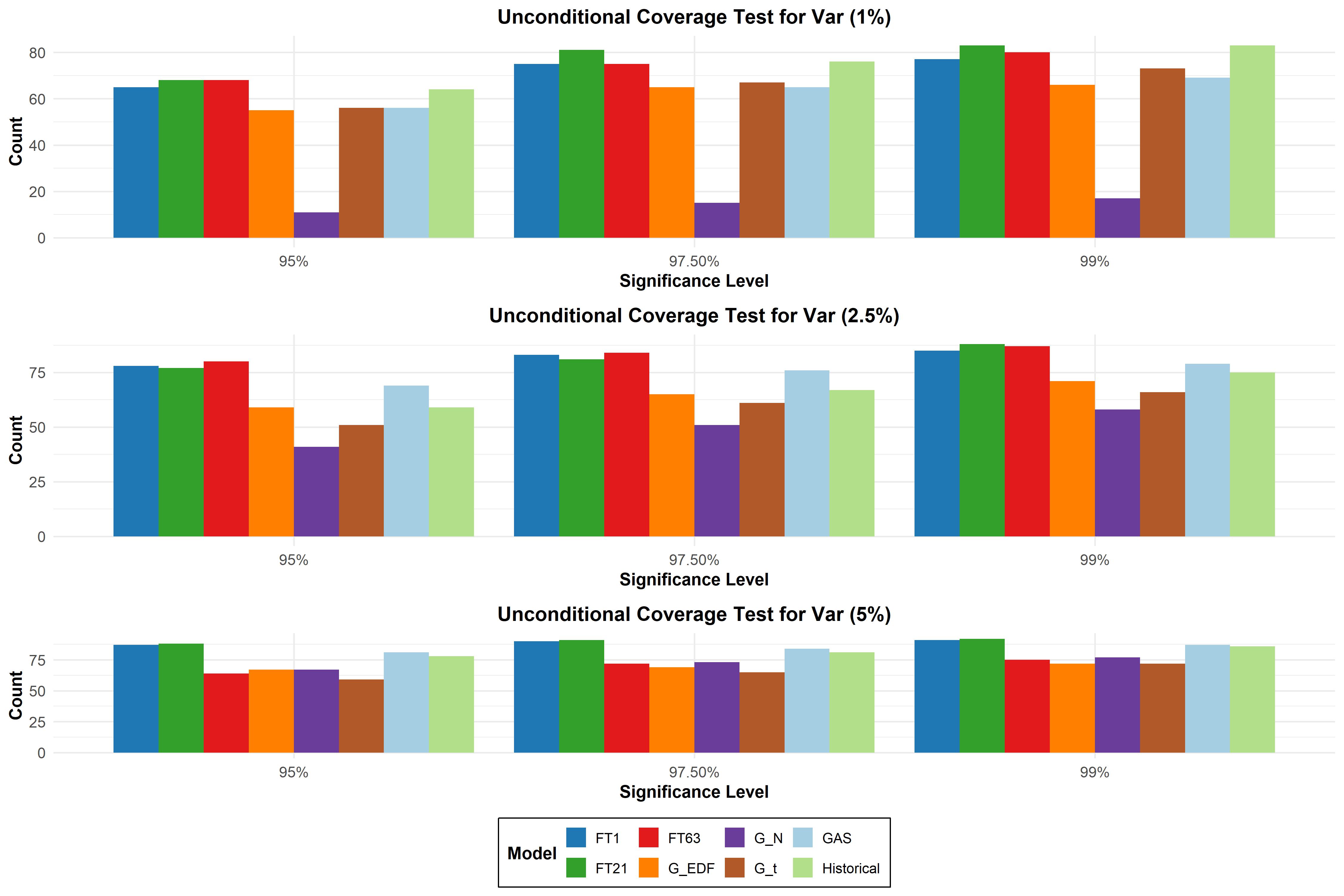
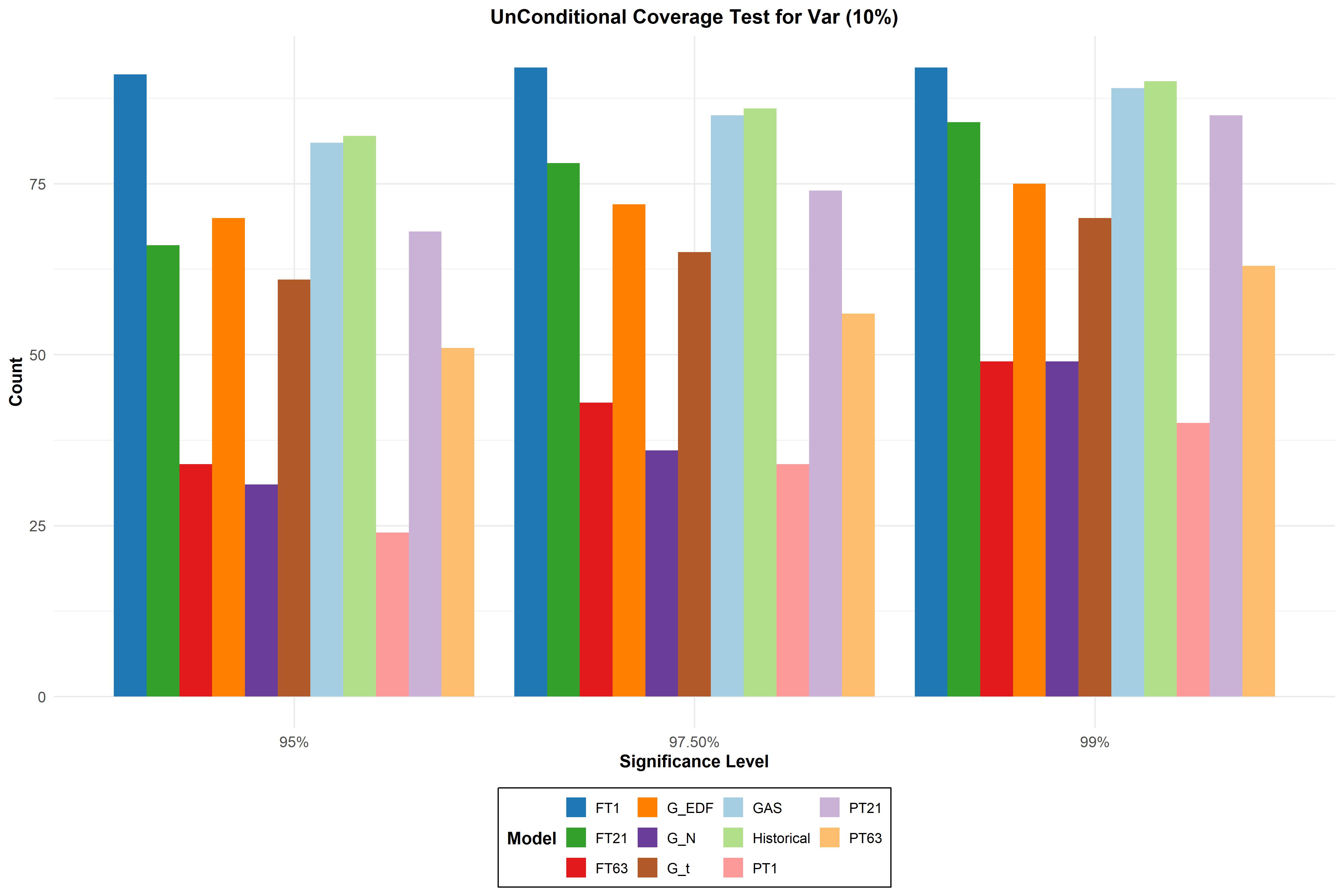
Figure A.1: This figure shows the bar plots of number of assets (out of 92) for which we failed to reject the null hypothesis in the Unconditional Coverage (UC) test at various Value at Risk (VaR) levels. A higher number indicates better model performance, as it reflects a closer alignment between observed and expected VaR violations for each specified model. Results are reported for four VaR confidence levels (1%, 2.5%, 5%, and 10%) across different models.

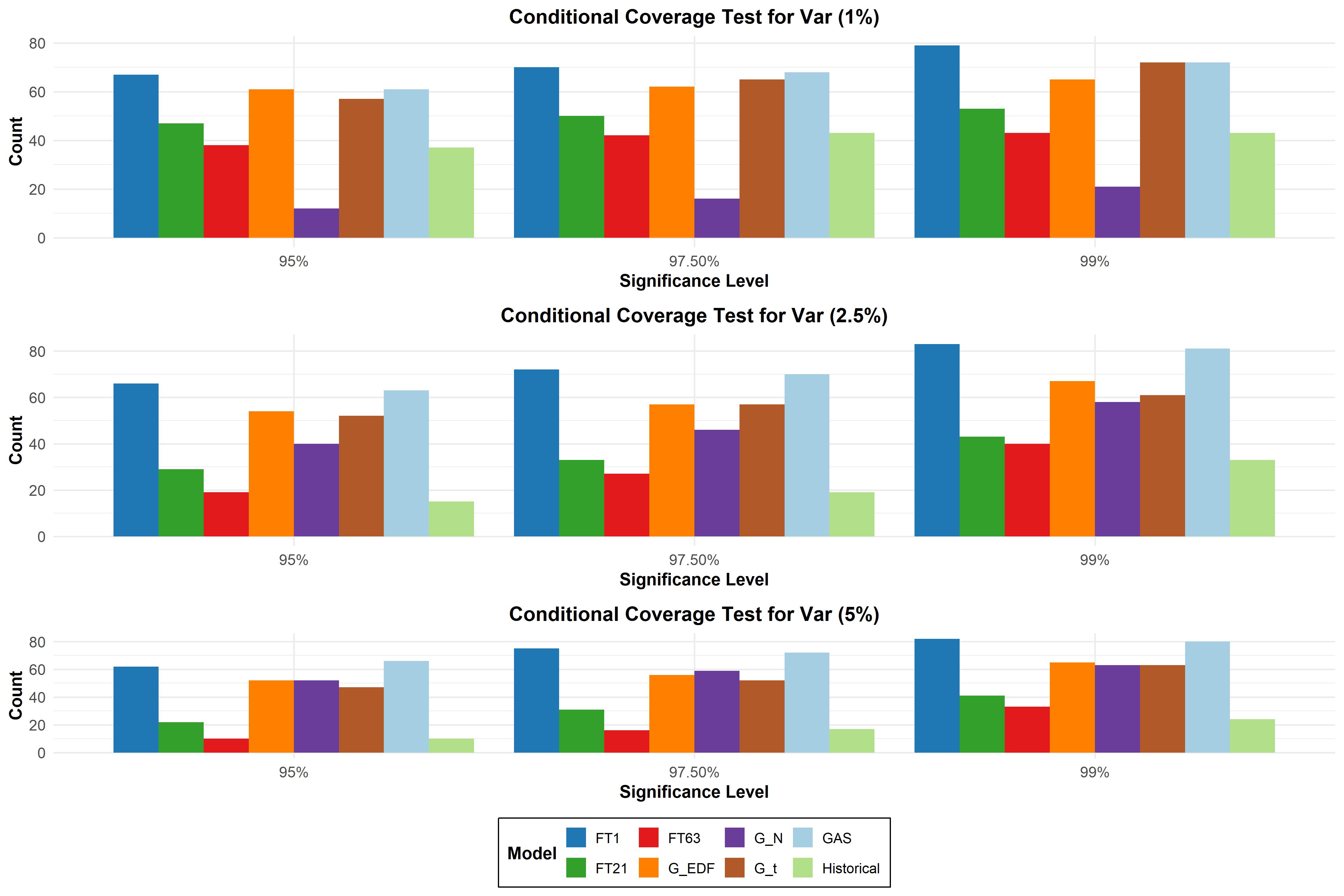
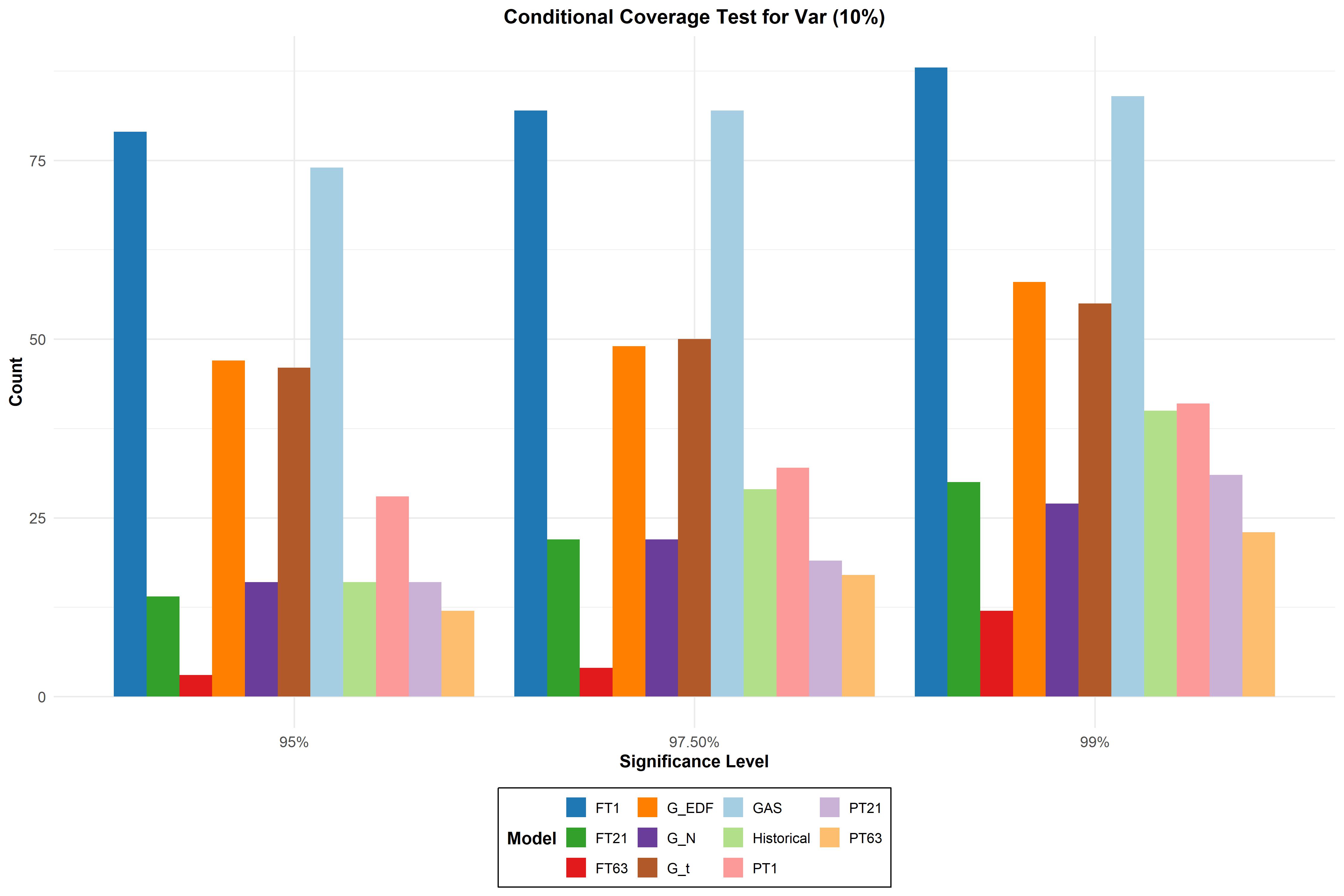
Figure A.2: This figure shows the bar plot of the number of assets (out of 92) for which we failed to reject the null hypothesis in the Conditional Coverage (CC) test at various Value at Risk (VaR) levels. A higher number indicates better model performance, as it reflects a closer alignment between observed and expected VaR violations for each specified model. Results are reported for four VaR confidence levels (1%, 2.5%, 5%, and 10%) across different models.

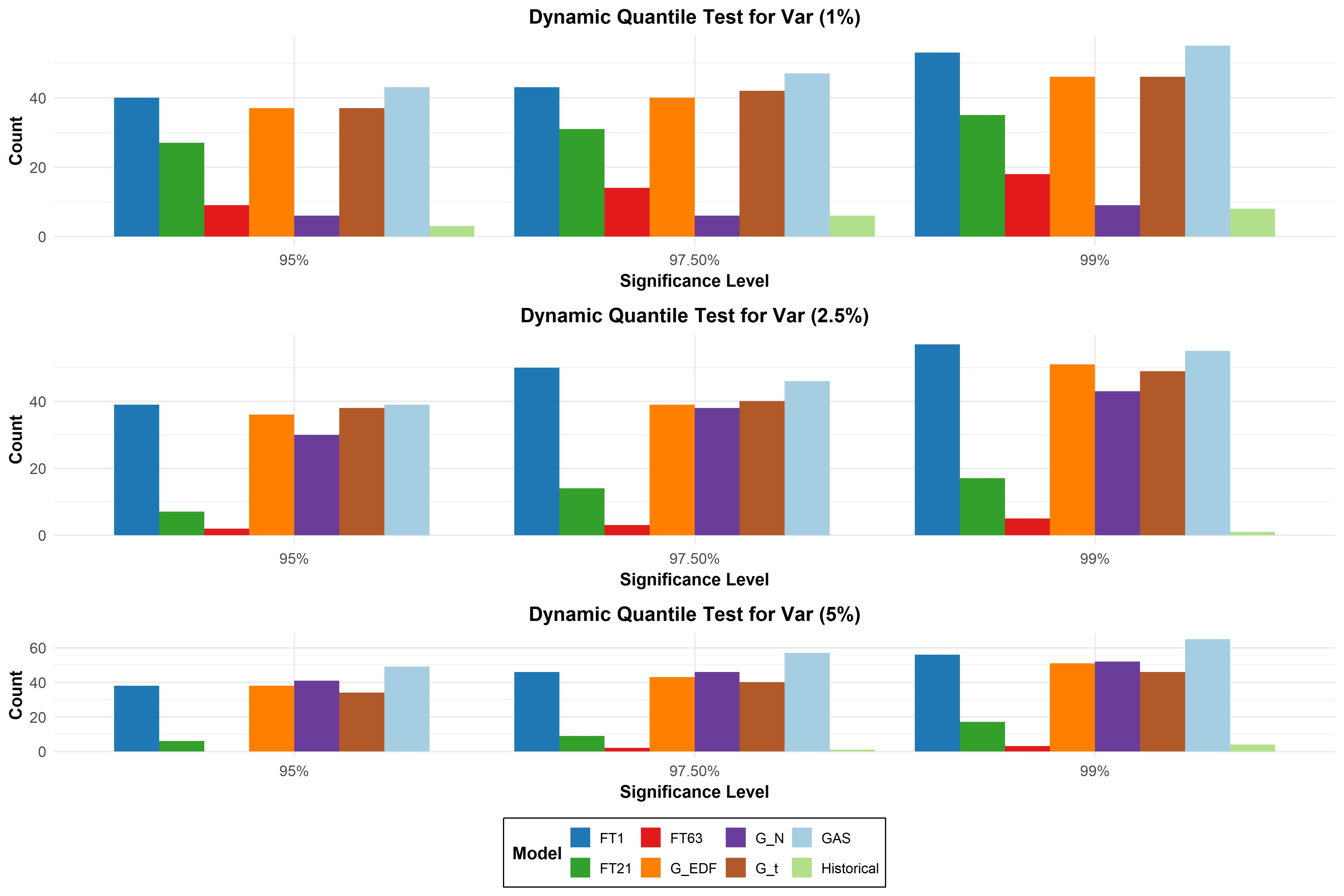
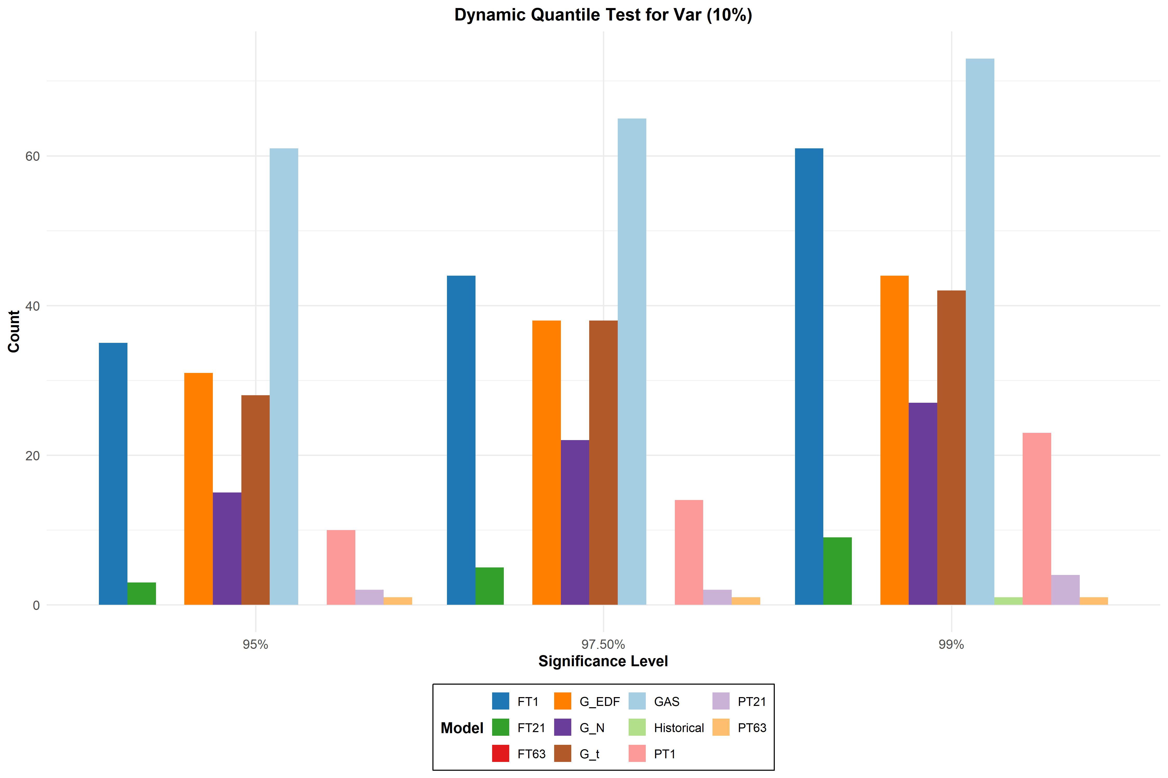
Figure A.3: This figure shows the bar plot of the number of assets (out of 92) for which we failed to reject the null hypothesis in the Dynamic Quantile (DQ) test at various Value at Risk (VaR) levels. A higher number indicates better model performance, as it reflects a closer alignment between observed and expected VaR violations for each specified model. Results are reported for four VaR confidence levels (1%, 2.5%, 5%, and 10%) across different models.

References

- Angelidis et al. (2004) Angelidis, T., Benos, A., Degiannakis, S., 2004. The use of GARCH models in VaR estimation. Statistical Methodology 1, 105–128.
- Athey et al. (2021) Athey, S., Imbens, G.W., Metzger, J., Munro, E., 2021. Using wasserstein generative adversarial networks for the design of monte carlo simulations. Journal of Econometrics , 105076.
- Bommasani et al. (2021) Bommasani, R., Hudson, D.A., Adeli, E., Altman, R., Arora, S., von Arx, S., Bernstein, M.S., Bohg, J., Bosselut, A., Brunskill, E., et al., 2021. On the opportunities and risks of foundation models. arXiv preprint arXiv:2108.07258 .
- Chakraborty et al. (2024) Chakraborty, N., Ornik, M., Driggs-Campbell, K., 2024. Hallucination detection in foundation models for decision-making: A flexible definition and review of the state of the art. arXiv preprint arXiv:2403.16527 .
- Chen et al. (2024) Chen, L., Pelger, M., Zhu, J., 2024. Deep learning in asset pricing. Management Science 70, 714–750.
- Christensen et al. (2023) Christensen, K., Siggaard, M., Veliyev, B., 2023. A machine learning approach to volatility forecasting. Journal of Financial Econometrics 21, 1680–1727.
- Christoffersen (1998) Christoffersen, P.F., 1998. Evaluating interval forecasts. International Economic Review 39, 841–862.
- Creal et al. (2013) Creal, D., Koopman, S.J., Lucas, A., 2013. Generalized autoregressive score models with applications. Journal of Applied Econometrics 28, 777–795.
- Das et al. (2024) Das, A., Kong, W., Sen, R., Zhou, Y., 2024. A decoder-only foundation model for time-series forecasting. arXiv preprint arXiv:2310.10688 .
- Diebold and Mariano (2002) Diebold, F.X., Mariano, R.S., 2002. Comparing predictive accuracy. Journal of Business & Economic Statistics 20, 134–144.
- Ehm et al. (2016) Ehm, W., Gneiting, T., Jordan, A., Krüger, F., 2016. Of quantiles and expectiles: consistent scoring functions, choquet representations and forecast rankings. Journal of the Royal Statistical Society Series B: Statistical Methodology 78, 505–562.
- Ericson et al. (2024) Ericson, L., Zhu, X., Han, X., Fu, R., Li, S., Guo, S., Hu, P., 2024. Deep generative modeling for financial time series with application in var: A comparative review. arXiv preprint arXiv:2401.10370 .
- Fissler and Ziegel (2016) Fissler, T., Ziegel, J.F., 2016. Higher order elicitability and Osband’s principle. The Annals of Statistics 44, 1680 – 1707. doi:10.1214/16-AOS1439.
- Garza and Mergenthaler-Canseco (2024) Garza, A., Mergenthaler-Canseco, M., 2024. Timegpt-1. arXiv preprint arXiv:2310.03589 .
- Gneiting (2011) Gneiting, T., 2011. Making and evaluating point forecasts. Journal of the American Statistical Association 106, 746–762.
- González-Rivera et al. (2004) González-Rivera, G., Lee, T.H., Mishra, S., 2004. Forecasting volatility: A reality check based on option pricing, utility function, value-at-risk, and predictive likelihood. International Journal of Forecasting 20, 629–645.
- Gu et al. (2020) Gu, S., Kelly, B., Xiu, D., 2020. Empirical asset pricing via machine learning. The Review of Financial Studies 33, 2223–2273.
- Guijarro-Ordonez et al. (2021) Guijarro-Ordonez, J., Pelger, M., Zanotti, G., 2021. Deep learning statistical arbitrage. arXiv preprint arXiv:2106.04028 .
- Hofert et al. (2022) Hofert, M., Prasad, A., Zhu, M., 2022. Multivariate time-series modeling with generative neural networks. Econometrics and Statistics 23, 147–164.
- Hoga and Demetrescu (2023) Hoga, Y., Demetrescu, M., 2023. Monitoring value-at-risk and expected shortfall forecasts. Management Science 69, 2954–2971.
- Kupiec (1995) Kupiec, P., 1995. Techniques for verifying the accuracy of risk measurement models. The Journal of Derivatives 3, 73 – 84.
- Makridakis et al. (2020) Makridakis, S., Spiliotis, E., Assimakopoulos, V., 2020. The M4 competition: 100,000 time series and 61 forecasting methods. International Journal of Forecasting 36, 54–74.
- Manganelli and Engle (2004) Manganelli, S., Engle, R.F., 2004. A comparison of value-at-risk models in finance. Risk measures for the 21st century , 123–143.
- Mikkilä and Kanniainen (2023) Mikkilä, O., Kanniainen, J., 2023. Empirical deep hedging. Quantitative Finance 23, 111–122.
- Nareklishvili et al. (2023) Nareklishvili, M., Polson, N., Sokolov, V., 2023. Generative causal inference. arXiv preprint arXiv:2306.16096 .
- Patton et al. (2019) Patton, A.J., Ziegel, J.F., Chen, R., 2019. Dynamic semiparametric models for expected shortfall (and value-at-risk). Journal of Econometrics 211, 388–413.
- Rasul et al. (2023) Rasul, K., Ashok, A., Williams, A.R., Khorasani, A., Adamopoulos, G., Bhagwatkar, R., Biloš, M., Ghonia, H., Hassen, N.V., Schneider, A., et al., 2023. Lag-llama: Towards foundation models for time series forecasting. arXiv preprint arXiv:2310.08278 .
- Spiliotis et al. (2020) Spiliotis, E., Kouloumos, A., Assimakopoulos, V., Makridakis, S., 2020. Are forecasting competitions data representative of the reality? International Journal of Forecasting 36, 37–53.
- Taylor (2005) Taylor, J.W., 2005. Generating volatility forecasts from value at risk estimates. Management Science 51, 712–725.
- Taylor (2019) Taylor, J.W., 2019. Forecasting value at risk and expected shortfall using a semiparametric approach based on the asymmetric Laplace distribution. Journal of Business & Economic Statistics 37, 121–133.
- Tran et al. (2018) Tran, D.T., Iosifidis, A., Kanniainen, J., Gabbouj, M., 2018. Temporal attention-augmented bilinear network for financial time-series data analysis. IEEE Transactions on Neural Networks and Learning Systems 30, 1407–1418.
- Tran et al. (2019) Tran, D.T., Kanniainen, J., Gabbouj, M., Iosifidis, A., 2019. Data-driven neural architecture learning for financial time-series forecasting. arXiv preprint arXiv:1903.06751 .