Analyzing (In)Abilities of SAEs via Formal Languages

Abstract

Autoencoders have been used for finding interpretable and disentangled features underlying neural network representations in both image and text domains. While the efficacy and pitfalls of such methods are well-studied in vision, there is a lack of corresponding results, both qualitative and quantitative, for the text domain. We aim to address this gap by training sparse autoencoders (SAEs) on a synthetic testbed of formal languages. Specifically, we train SAEs on the hidden representations of models trained on formal languages (Dyck-2, Expr, and English PCFG) under a wide variety of hyperparameter settings, finding interpretable latents often emerge in the features learned by our SAEs. However, similar to vision, we find performance turns out to be highly sensitive to inductive biases of the training pipeline. Moreover, we show latents correlating to certain features of the input do not always induce a causal impact on model’s computation. We thus argue that causality has to become a central target in SAE training: learning of causal features should be incentivized from the ground-up. Motivated by this, we propose and perform preliminary investigations for an approach that promotes learning of causally relevant features in our formal language setting.

Analyzing (In)Abilities of SAEs via Formal Languages

Abhinav Menon IIIT Hyderabad abhinav.m@research.iiit.ac.in                        Manish Shrivastava IIIT Hyderabad m.shrivastava@iiit.ac.in

David Krueger MILA david.scott.krueger@gmail.com                        Ekdeep Singh Lubana CBS, Harvard University ekdeeplubana@fas.harvard.edu

1 Introduction

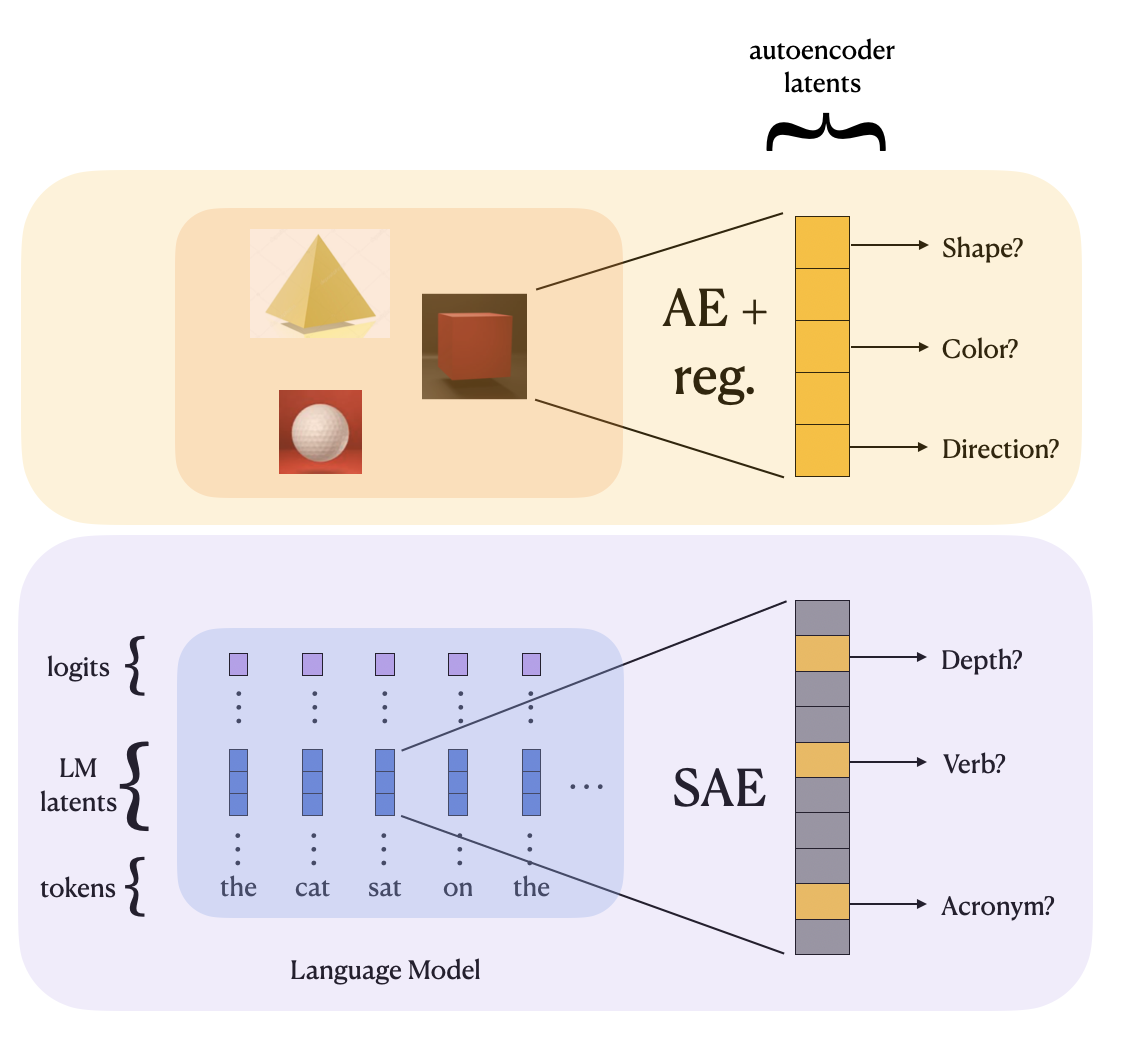
Figure 1: The autoencoder paradigm for interpretability. Autoencoders have formed the basis of approaches to disentanglement in the vision domain (Higgins et al., 2017). Utilizing synthetic testbeds, prior work has shown several limitations in this general pipeline Locatello et al. (2019); Träuble et al. (2021). While SAEs have similarly been used to disentangle hidden representations of language models for interpretability, we aim to perform a similar study as ones in vision to understand the (in)abilities of SAEs.

In recent years, mechanistic interpretability has gained currency as an approach towards understanding the functioning of language models (LMs) Nanda et al. (2023); Olsson et al. (2022); Wang et al. (2022); Li et al. (2024a). A mechanistic interpretability paradigm that has seen remarkable progress especially is sparse autoencoders (SAEs), which aims to disentangle model representations into independent, interpretable components Lieberum et al. (2024); Bricken et al. (2023); Cunningham et al. (2023); Engels et al. (2024); Gao et al. (2024); Marks et al. (2024); Rajamanoharan et al. (2024) (see App. A for related work). Similar interpretability approaches based on autoencoders have been extensively studied in the vision domain (see Fig. 1), from both empirical and theoretical viewpoints Locatello et al. (2019); Träuble et al. (2021); Lachapelle et al. (2023); Locatello et al. (2020); Klindt et al. (2020). Specifically, using synthetic testbeds where a ground-truth set of latents underlying the data-generating process can be listed Higgins et al. (2017), these studies have established results on the (non-)identifiability of disentangled representations via autoencoders and argued for the importance of inductive biases, which motivate different regularization terms. We argue a similar study is needed for understanding the (in)abilities of SAEs for interpreting LM representations.

This work. We propose the use of synthetic language testbeds to stress-test the SAE approach to interpretability of LMs. In particular, we train a spectrum of SAEs on a set of formal languages—specifically, probabilistic context free grammars (Dyck-2, Expr, and English)—and demonstrate interpretable latents that activate for relevant concepts of the data-generating process (e.g., parts-of-speech) are easily identifiable. However, similar to vision, we find results are highly sensitive to the training pipeline, with identified latents rarely having a causal impact on the model output. This indicates new approaches that directly target learning of causally relevant latents are needed. To take a step in this direction, we thus propose a training pipeline that exploits token-level correlations as “weak supervision” (Locatello et al., 2020). Overall, our contributions can be summarized as follows.

• We define formal languages of different complexities, train Transformers on these languages, and then analyze SAEs trained on their representations under several different hyperparameter settings. We identify several features occurring in these SAEs that correspond to variables central to the data generating process; e.g., depth and part of speech (Sec. 2).

• We demonstrate, inline with results from vision, that identifiability of disentangled features is not robust (Sec. 3). Results are highly sensitive to changes in normalization methods, hyperparameters, and other such settings. For example, models trained under $L_{1}$ regularization consistently fail to find interpretable features; additionally, normalization has widely varying effects on the reconstruction capabilities of the SAEs.

• We demonstrate that mere identification of disentangled features does not imply said features are causally relevant to the model’s computation (Sec. 3.3). This indicates causality should be actively modeled as a constraint in the training pipeline of SAEs. We take a step towards this objective by proposing a modified SAE training protocol that deems correlations between tokens as naturally available interventions, similar to use of correlated images in autoencoder based approach for vision interpretability (Locatello et al., 2020; Klindt et al., 2020; Brehmer et al., 2022). Results show that the proposed protocol often yields latents with interpretable and causal impact on model outputs in our formal language setting (Sec. 4). These results can be deemed a proof-of-concept demonstration that insights from prior work on autonencoder-based interpretability may continue to be useful for LM settings as well.

2 Experimental Setup

Our experiments consist of training SAEs (of various paradigms) on the intermediate representation of transformer models trained on formal languages. We explain the data generating process, model architectures, and training paradigms next.

2.1 Data and Models

The formal languages we work with are probabilistic context-free grammars (PCFGs), which are generated by starting with a fixed ‘start’ symbol, and probabilistically replacing nonterminals according to production rules. We work with three PCFGs, intended to represent levels of complexity (in parsing and generation). In order of increasing complexity, the languages we consider are Dyck-2 (the language of all matched bracket sequences with two types of brackets), Expr (a language of prefix arithmetic expressions), and English (a simple fragment of English syntax with only subject-verb-object constructions). See App. B for precise details.

We train Transformers Karpathy (2022) via the standard autoregressive language modeling pipeline on each of the above languages. The models have 128-dimensional embeddings, with 4 attention heads and MLPs, and 2 blocks. In all cases, the models achieve more than 99% validity, i.e., under stochastic decoding, the strings generated belong to the language more than 99% of the time.

2.2 SAE Architecture

Broadly, we use the conventional SAE architecture, which consists of two linear layers (an encoder and a decoder transform) with an activation function in between. More explicitly, if the sizes of the input and hidden state are $d$ and $h$ respectively, then our SAEs implement functions of the type

$$\operatorname{SAE}(x)=W_{\text{dec}}(\sigma(W_{\text{enc}}(x)+b_{\text{enc}}))+b_{\text{dec}},$$

where $W_{\text{enc}}\in\mathbb{R}^{h\times d}$, $W_{\text{dec}}\in\mathbb{R}^{d\times h}$, and $b_{\text{enc}}\in\mathbb{R}^{h},b_{\text{dec}}\in\mathbb{R}^{d}$. We pick $h$ from $\{d,2d,4d,8d\}$ and $\sigma=\text{ReLU}$ as the activation function. We refer to the encoder transform (up to and including the nonlinearity) as $E$, the decoder as $D$, and the hidden representation (the output of the encoder) as a latent. When these latents have interpretable explanations, identified correlationally (Sec. 3.1), we also refer to them as features.

Training is performed by optimizing on the MSE between $x$ and $\operatorname{SAE}(x)$, where the input $x$ to the SAEs is the output of the first block of the Transformer model. Sparsity is enforced via two main methods. The first (and most common in existing work) is an $L_{1}$-regularization term added to the loss, which encourages latent representations to have low $L_{1}$-norm. The hyperparameter for this method is the weight of the regularization term. We also use, following Gao et al. (2024), top-$k$ regularization—at the SAE hidden layer, after the activation, we select the highest $k$ latents, and zero out the rest. Effectively, we force the $L_{0}$-norm of the latents to be at most $k$, i.e., the hyperparameter is $k$ itself. We examine the effects of hyperparameters on the performance of SAEs in Sec. 3.2. We analyze variants of the architecture above by altering the normalization method and pre-bias. There are three parts of the operation of the SAE that can be normalized—the input, the reconstruction, and the decoder directions. This yields four architecture variants: no normalization (I), input and decoder with pre-bias (II), input alone (III), and input and reconstruction (IV). By pre-bias, we refer to the addition of a learnable vector $b_{\text{pre}}\in\mathbb{R}^{d}$ to the input before applying the encoder, which is then subtracted after applying the decoder.

2.3 Causality of Features

Given a trained SAE$:x\mapsto D(E(x))$, we examine the causality of the latents by defining a reconstructed run of the transformer. Let the model’s two layers be $L_{0}$ and $L_{1}$; then a normal run is $\text{logits}=W_{\text{LM}}L_{1}(L_{0}(t)),$ where $t\in\mathbb{R}^{s\times d}$ represents the embeddings of a sequence of $s$ tokens, and $W_{\text{LM}}\in\mathbb{R}^{d\times|V|}$ is the projection of the final representations into the logit space. The prediction of the next token is given, therefore, by $\operatorname{softmax}(\text{logits})$. We then define a reconstructed run as $\text{logits}=W_{\text{LM}}L_{1}(D(E(L_{0}(t))));$ i.e., we interrupt the run after the first layer, pass the output through the SAE, and resume the run using the reconstruction of the SAE. For ease of notation, we partition the reconstructed run into two functions, which chained together give the complete run:

$$f:=E\circ L_{0};\quad g:=W_{\text{LM}}\circ L_{1}\circ D.$$

Thus, the latent of a token $x$ is given by $f(x)$ and the logit distribution of a token with latent $l$ is given by $g(l)$. To study the causality of the representations, then, we intervene on the latent representation, between $E$ and $D$ (in other words, between $f$ and $g$). We intervene on the specific elements of the latent that correlate with interpretable features of the input tokens; for instance, in the English grammars, we search for latents correlating with each part of speech in the grammar. Our interventions consist of ‘clamping’ latents to some fixed value. In other words, for each token, we run the forward pass and extract the latent representation; we set certain elements to a clamp value, leaving the rest unchanged—this value is then passed through the decoder $D$ and the rest of the forward pass.

Figure 2: A feature matching corresponding opening and closing brackets. Each line represents a pair of brackets, and joins the opening bracket’s activation (left) to the closing bracket’s (right). We note that the depth and opening activation are sufficient to determine the closing activation, and that the opening and closing activations are sufficient to determine the depth.

We examine the effects of the interventions at the sentence level (Sec. 3.3). This is done in the context of free generation, where the model is prompted by a <BOS> token, and the above intervention is run on each token’s representation. We intervene using values spaced at 10 equal intervals in $[-v_{\text{max}},v_{\text{max}}]$, where $v_{\text{max}}$ is the maximum absolute value attained by the intervened feature. We use both positive and negative values to account for the possibility that the feature may be antipodal to our explanation.

In Sec. 4, we incentivize the SAEs to identify features with causal function by adding a regularization term (Fig. 6). We carry out the same studies noted above for those SAEs and qualitatively connect them to the nature of regularization (Sec. 4.3).

3 Results

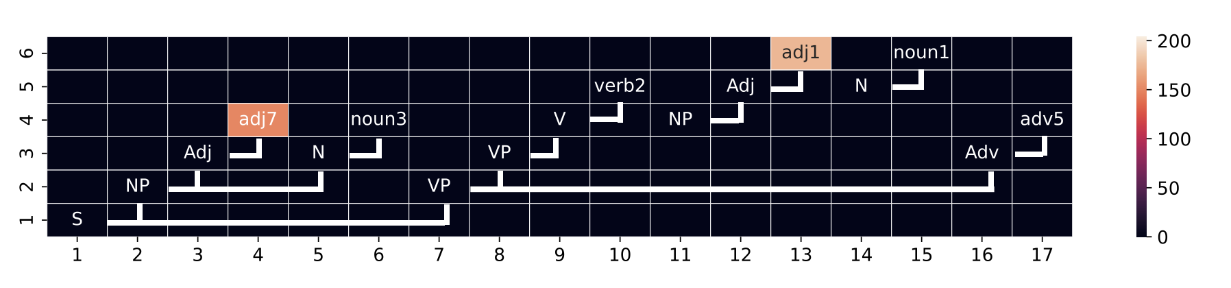
Figure 3: A feature that activates only on adjectives, at any position. Here, depth is represented by the y-axis and position by the x-axis; the lines connect nonterminals to their productions (see App. B for the production rules). The cell color represents the activation magnitude.

3.1 Do SAEs Find Features?

Qualitatively, we observe that top-$k$-regularized SAEs tend to have more interpretable features than $L_{1}$-regularized ones. The former results in interpretable features across all languages—we find features representing fundamental aspects of the corresponding grammars, as discussed next briefly. See App. C for further results, including other features we are able to identify and how strongly features correlate with their claimed explanations.

In the case of Dyck-2, we expect the depth (the number of brackets yet to be closed) to be represented. We find a feature that thresholds the depth of tokens, i.e., it activates on tokens with depth above a certain threshold depth $D$. Usually, $D$ is greater than the mean; for instance, when mean depth is 8.3, we find $D=11$. We also find features that match corresponding pairs of opening and closing brackets, usually at lower depths (Fig. 2). These features take values from only a few small ranges, and their values at an opening bracket determine those they take at the matching closing bracket. These features, even though they are binary, indicate that the token representations do maintain some form of counter (which aligns with claims from prior work, like Bhattamishra et al. (2020)).

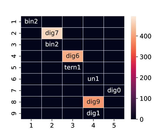
Figure 4: A feature that activates when exactly one more expression is required. Here, the x-axis is token depth, and the y-axis is token index. The lines connect the operators to their operands.

In Expr, the analogue of depth is a counter that indicates how many more expressions are needed to complete the sequence (App. B). We find a feature that activates exactly when this counter’s value is 1, i.e., when exactly one expression is required (Fig. 4). This provides strong evidence of a counter process being implemented; in fact, we note that generation without this process would be rather convoluted (Algorithm 1).

An inference we can make from the Expr features is that there is an implicit “type” feature in the representations, distinguishing operators of different valences. A natural place to look for this is the parts of speech in our English grammar, and we find that $k$-regularized SAEs do contain features corresponding to each part of speech. For example, we illustrate the ‘adjective’ feature in Fig. 3.

Further, we note a scaling relation in the performance of the top-$k$-regularized SAEs with hidden dimension size. The reconstruction loss they achieve (after a fixed number of iterations) decreases according to a power law with the size of the autoencoder’s hidden layer (see App. F); similar results were seen by Sharkey et al. (2024), relating the reconstruction loss to the L1 penalty coefficient, indicating our setup captures part of the phenomenology observed with complex settings.

Language	$L_{1}$				top-$k$
	I	II	III	IV	I	II	III	IV
Dyck-2	0.01	0.0	0.01	0.0	49.27	3.48	50.02	0.06
Expr	33.31	6.50	0.06	0.49	99.88	69.14	99.76	0.0
English	0.29	1.13	0.01	0.01	92.46	50.12	80.79	0.37

Table 1: Sensitivity to Hyperparameters. Reconstruction Accuracy (%) averaged over regularization values and hidden size. We present the accuracies for SAEs with no normalization (I); with inputs and decoder normalized, and pre-bias (II); with inputs normalized (III); and with inputs and reconstructions normalized (IV). The reconstruction capabilities of the models shows high variance across hyperparameter settings.

Input Sequence	#Required	Clamp $-v_{\text{max}}$	Clamp 0	Clamp $v_{\text{max}}$
un2 tern1 dig8 bin0 tern2 bin2 bin2 dig6 dig7 dig5	4	4	4	4
bin1 un1 tern1 bin2 dig0 dig7 dig0 bin1 dig3 dig7	1	1	1	1
un0 tern1 dig9 dig7 un0 tern1 un2 bin2 dig6 dig6	2	2	2	2
tern1 dig1 dig7 tern1 tern1 dig7 tern1 tern1 un0 un1	8	8	8	8

Table 2: Behavior of the Expr model under interventions. The ‘clamp’ columns indicate the number of expressions generated by the model after being prompted by the input sequence and an intervention defined by the clamp value. We see that there is no effect of the intervention on the behavior of the model.

3.2 Are SAEs Robust to Hyperparameters?

As noted before, we find top-$k$-regularized SAEs consistently yield more interpretable features languages than $L_{1}$-regularized SAEs. We also measure the reconstruction accuracy, or the percentage of valid generations of the model after the latents are substituted with the SAE reconstructions. Tab. 1 shows the average results for each combination of regularization, pre-bias, and normalization strategy (averaged across regularization values and hidden sizes). We see that top-$k$-regularized SAEs usually (but not always) outperform $L_{1}$-regularized ones if all other settings are kept the same. We also note from this table the high sensitivity to hyperparameter settings that SAEs exhibit: no clear trend is visible across languages, regularization methods, or normalization settings—inline with Locatello et al. (2019)’s findings.

3.3 Does Correlation Imply Causation?

An interesting aspect of the features we identify is that despite strongly correlating with the discussed explanation (see Tab. 3), they do not have the expected causal effects. In this section, we outline our findings in causal experiments (Sec. 2.3) on the features described above.

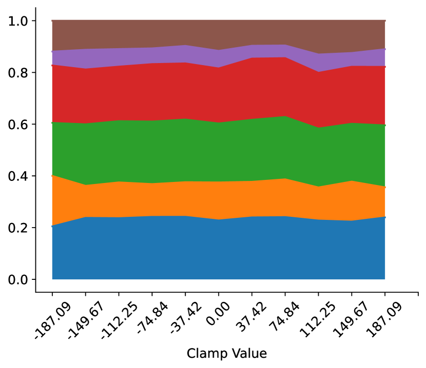
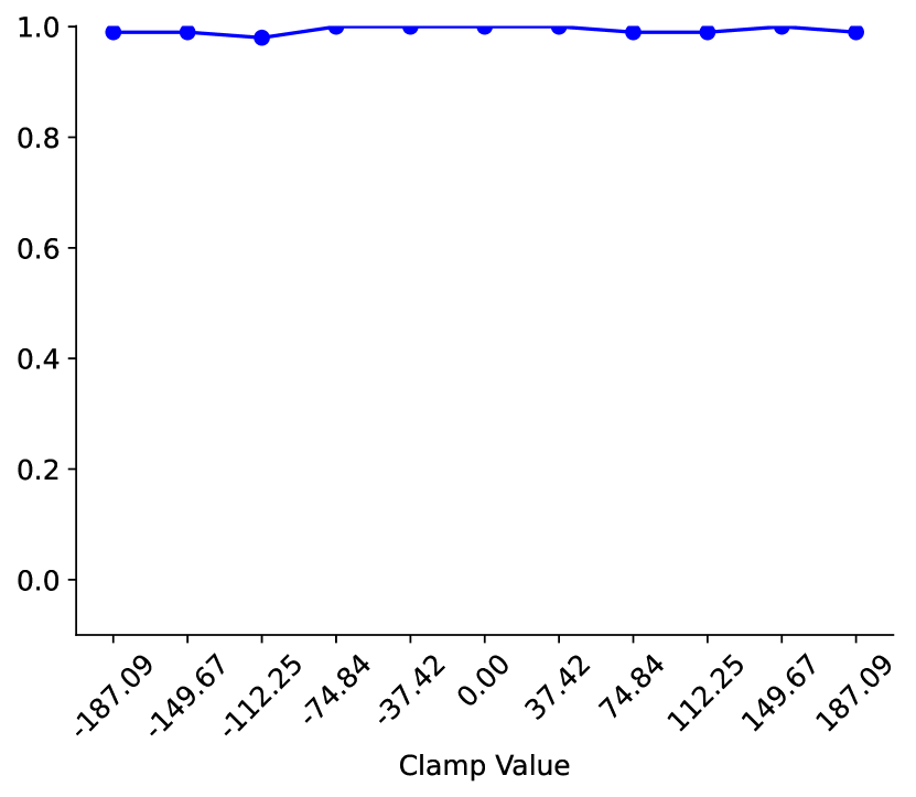
Figure 5: Behavior of the English model under interventions. We intervene on the model by replacing its hidden representations with the SAE’s reconstructions, where an SAE latent (specifically, one corresponding to adjectives) is clamped to a fixed value. These values are selected at uniform intervals from $[-v_{\text{max}},v_{\text{max}}]$, where $v_{\text{max}}$ is the maximum value taken by that latent (inline with Templeton et al. (2024)). For each value (x-axis), we plot the fraction of each part of speech (nouns, pronouns, adjectives, verbs, adverbs, and conjunctions) in the output (left) and the fraction of outputs that are grammatical (right). We see interventions yield essentially no visible effects.

In the case of Expr, we have seen in Sec. 3.1 that there is a counter feature that activates when exactly one expression is left to complete the sequence. We pass an incomplete sequence to the model, and intervene on this feature by clamping it to one of $\{-v_{\text{max}},0,v_{\text{max}}\}$, where $v_{\text{max}}$ is the maximum absolute value of the latent (see Sec. 2.3). We then examine the generations that result in each case. We expect that high clamp values will cause the model to generate only one more expression (even if more may be required) and low values will cause it to generate more than one, or perhaps end the sequence immediately (even if exactly one is needed); or vice versa, since we cannot be certain of the direction to apply intervention in. Tab. 2 presents the results of this experiment. For each input sample, we mention the number of expressions required to complete it, and the number of expressions actually generated by the model under each intervention. We do not see the expected—or indeed any—causal effect of intervening on this feature—it appears that this feature is only correlational in nature.

Similarly, we examine our English grammar. Here, we examine the effects of intervening on the part-of-speech features described in Sec. 3.1. Note that for a feature correlating with, say, adjectives, we can expect that if it has a causal effect, it must control the next-token distribution for that part-of-speech (as this is the only task the model is trained on). We thus apply our causality protocol (Sec. 2.3) to the feature correlating with adjectives. The results of this experiment are shown in Fig. 5. In this case, as in Expr, we do not see a causal effect of intervening on this feature. See App. D for similar results on other parts-of-speech.

4 Incentivizing Causality

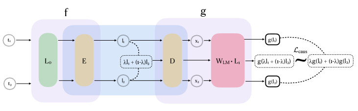
Figure 6: Operationalizing the causal regularization term. A clean run of the model consists of applying $L_{0}$, followed by $L_{1}$ and $W_{\text{LM}}$. We define a reconstructed run, which introduces an SAE between these two layers. The SAE consists of an encoder $E$ and a decoder $D$. We denote the input embeddings as $t$, SAE latents as $l$, and reconstructed model activations as $x$. Furthermore, we group the first part of the reconstructed run as $f:=E\circ L_{0}$, and the second part as $g:=W_{\text{LM}}\circ L_{1}\circ D$. Given two tokens $t_{1}$ and $t_{2}$, we interpolate between the latents $l_{1}$ and $l_{2}$ (indicated by a dotted line) and pass this as input to $g$; our causal loss $\mathcal{L}_{\text{caus}}$ is then given by the difference between the interpolation of the outputs, and the output of the interpolation.

Our results above indicate that though SAEs are competent at identifying features correlated with semantically meaningful concepts, these features may not have the expected (or any) causal effects. This mirrors similar observations made in vision, where it has been noted (Locatello et al., 2019) that mere data reconstruction pipelines (e.g., based on autoencoders) can fail to disentangle the latent factors of a generative model. However, later work on the topic demonstrated that correlations in the data-generating process (e.g., correlation in nearby frames of a video) can be leveraged to obtain disentangled representations (Locatello et al., 2020; Klindt et al., 2020). As this method relies on supervision via other data samples, rather than a ground truth, it is described as weak supervision. A warranted question then is whether weak supervision can be elicited in language modeling scenarios too.

Motivated by the above, we take inspiration from Klindt et al. (2020)’s use of temporal correlations in video data as weak supervision. We argue the temporal and sequential nature of language can be exploited in a similar manner as well: more precisely, we can consider tokens belonging to the same sequence to share latent factors, and therefore pair up tokens within sequences in a similar way as image pairs in vision. We next operationalize this idea in our setup (Sec. 4.1) and then analyze the features obtained by SAEs trained with this method (Sec. 4.2). We discuss in Sec. 4.3 the connection between the inductive biases of the proposed pipeline and the nature of identified features. We note that the proposed protocol and results should be deemed a proof-of-concept: our goal is to make a stronger connection to prior literature on autoencoder-based approaches to interpretability, hence eliciting (in)abilities of such protocols.

4.1 Defining Causal Loss

We propose an additional causal regularization term in the loss to incentivize causality. Thus, we now have a loss function given by

$$\mathcal{L}=\mathcal{L}_{\text{recon}}+\alpha\mathcal{L}_{\text{sparse}}+\beta\mathcal{L}_{\text{caus}}.$$

In order to define $\mathcal{L}_{\text{caus}}$, note that what we want is for interventions on the latents to lead to interpretable changes in the model output. However, we do not want the changes to be arbitrary, i.e., we cannot simply try to maximize the change caused by an ablation—then the incentive for disentanglement is harmed. We therefore introduce weak supervision, motivated by the ‘match pairing’ approach of Locatello et al. (2020); Klindt et al. (2020).

Specifically, we try to make the run (forward pass) of the model on a given token $t_{1}$ similar to its run on a different, albeit related, token $t_{2}$. More precisely, given a single token $t_{1}$, we try to intervene on its latent representation $l_{1}$ to cause its logit distribution to resemble that of $t_{2}$. We operationalize this by a simple interpolation technique—we intervene on $l_{1}$ during the reconstructed run (as defined in Sec. 2.3) of the model on $t_{1}$, replacing it with $\lambda\cdot l_{1}+(1-\lambda)\cdot l_{2}$ for some $\lambda\in[0,1)$. To define what to compare the output of the model on this corrupted run to be, we follow our intuition of using the run on $t_{2}$ as a form of supervision and compare the model output to the interpolation of the outputs of $t_{1}$ and $t_{2}$ (Fig. 6). This is similar to prior work that aims to improve the robustness of representations and obtain smoother decision boundaries by training on interpolations of inputs (Verma et al., 2019). Another way to motivate this operationalization is that we would like to force the model to change its output based on specific, surgical changes in the latents that happen as tokens evolve over time.

More formally, let $a\overset{\lambda}{\leftrightarrow}b$ denote the interpolation $\lambda a+(1-\lambda)b$ of vectors $a$ and $b$ by a scalar $\lambda$. Then we define the causal loss term for a token $t_{1}$, given a ‘baseline’ token $t_{2}$, as:

$$\mathcal{L}_{\text{caus}}(t_{1},t_{2}):=d\Big{(}g\left(l_{1}\overset{\lambda}{\leftrightarrow}l_{2}\right),g(l_{1})\overset{\lambda}{\leftrightarrow}g(l_{2})\Big{)},$$

where $d$ denotes MSE.

To pick $t_{2}$ in the pipeline above, we aim for as minimal an intervention as possible; this is to avoid the latent being completely overwritten, and to ensure that even small, surgical changes in the vicinity of the latent have causal effects. Thus we simply find the token with the latent nearest (by $L_{2}$ distance) to $l_{1}$. This is done at the sequence level; thus, for each sequence, we pair each token with the one nearest to it in the latent space, and find $\mathcal{L}_{\text{caus}}$ for each of these pairs. For $\lambda$, we simply sample from the uniform distribution over $[0,1]$ every iteration—this incentivizes causal effects for a wide range of interventions.

4.2 Nature of Causal Features

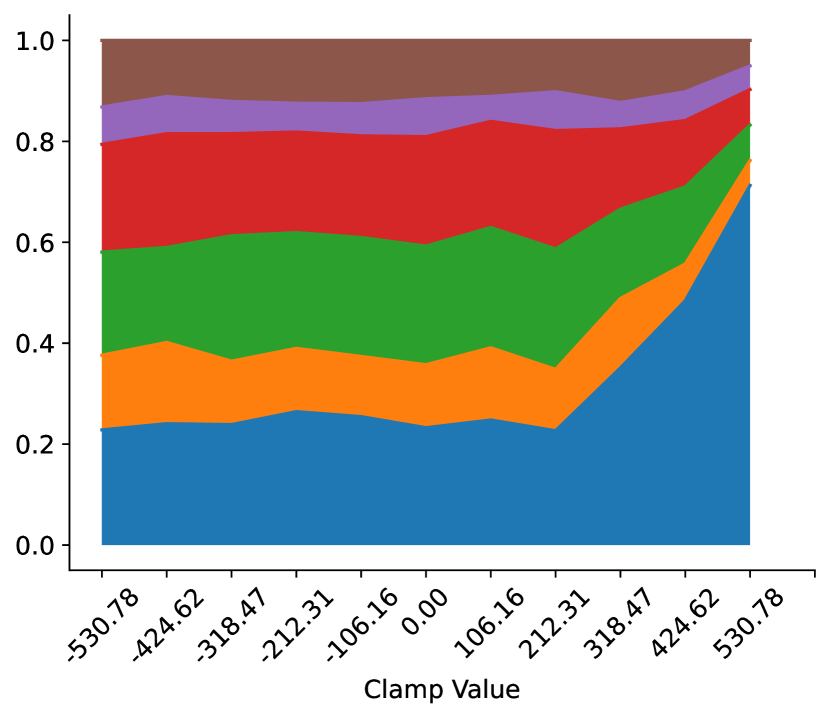
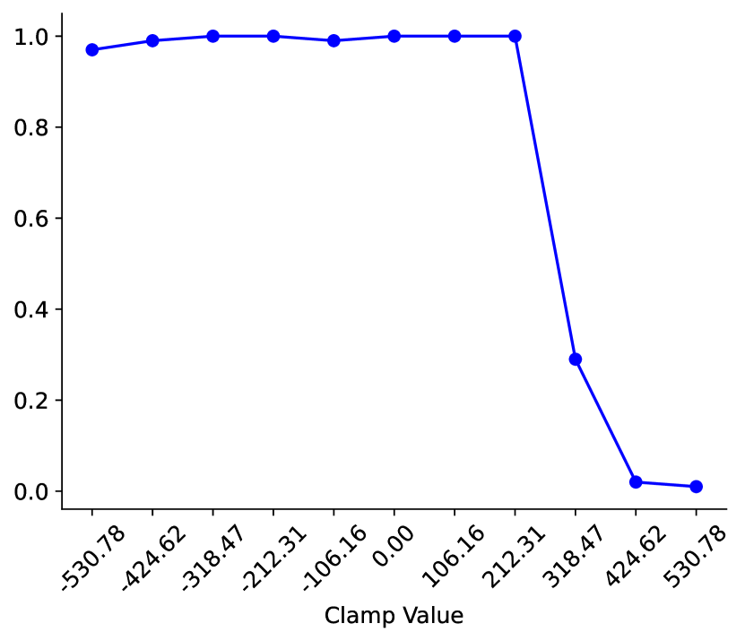
Figure 7: Behavior of the English model under interventions. We intervene on the model, replacing its hidden representations with the SAE’s reconstructions, clamping a single latent (in this case, the one corresponding to adjectives) to fixed value. These fixed values are selected at uniform intervals from $[-v_{\text{max}},v_{\text{max}}]$, where $v_{\text{max}}$ is the maximum value taken by that latent (inline with Templeton et al. (2024)). For each value of the clamp (x-axis), we plot the fraction of each part of speech (nouns, pronouns, adjectives, verbs, adverbs, and conjunctions) in the generated text (left) and the fraction of generations that are grammatical (right). We see that the SAEs trained with causal regularization have a predictable causal function.

As in the SAEs trained without this loss (Sec. 3.1), we identify a number of features correlating with parts of speech—specifically, adjectives, verbs and adverbs. Now, we predict that if these features have a monotonic causal function, they shift the output logit distribution towards the one predicted by the corresponding part of speech. For example, a feature correlating with adjectives should promote the probability of nouns being predicted next, as nouns are the only PoS allowed to come after adjectives (see App. B for the exact grammar). In the case of verbs, anything may appear as the next token except another verb; thus we expect the probability of verbs to be downweighted by this feature.

Fig. 7 presents the effect of these interventions on the PoS distribution across sentences, along with the grammaticality of generations. The effect is as we hypothesized. We also note that as soon as the distribution significantly shifts away from the uncorrupted distribution, the fraction of grammatical generations drops drastically. This supports, as pointed out in Träuble et al. (2021); Ahmed et al. (2020), the difficulty of learning disentangled representations from correlated data (in this case, with respect to PoS distribution and grammaticality). More examples of the causal function of these features can be found in App. D.3.

4.3 Inductive Biases in our Pipeline

As we remarked before, Locatello et al. (2019) demonstrated that finding latents underlying the data generating process is generally an ill-defined problem with multiple viable solutions. The authors thus argue that to the extent an approach achieves disentangled features, it is an inductive bias of the training pipeline. For example, their results show that a good deal of the variance in performance across paradigms (37%) can be accounted for by the effect of the objective function alone. In this section, therefore, we investigate the inductive biases of our approach. In particular, why do only certain parts of speech (adjectives, verbs and adverbs) have latents correlating with them when our causal loss term is introduced?

Figure 8: The computational graph of the second layer $L_{1}$ of the transformer model. Starting from the SAE latent $l$, the decoder $D$ produces a reconstruction of the model activation $x$; the blue box then represents $L_{1}$, whose output is projected by $W_{\text{LM}}$ into the logit space. The boldface arrows represent paths through the graph that involve fewer nonlinearities; our causal loss term incentivizes $D$ to write to the subspace of $x$ that is read by the modules in these paths.

To answer this, we reexamine the causal loss (Sec. 4.1). As $\overset{\lambda}{\leftrightarrow}$ represents a convex combination for all $\lambda\in[0,1]$, it effectively incentivizes the function $g$ to be distributive over convex combinations (i.e., over addition and scalar multiplication). In other words, it is an incentive for $g$ to be a linear function. This is of course not possible in full generality (else we would not need nonlinear models), but can work for features that have an approximately linear mapping to the output space.

In particular, consider the computational graph that $g$ represents (Fig. 8). Following the framework of Elhage et al. (2021), we consider the SAE decoder $D$ as writing to a subspace of $x\in\mathbb{R}^{d}$, which each of $\operatorname{attn}(x)$ and $\operatorname{MLP}(x)$ then read from. Now, note that the attention module involves two softmax operations, and is therefore a highly nonlinear operation. The MLP, by contrast, is a simple linear-GeLU-linear operation, and thus involves only one nonlinearity (which is in fact linear in the range $\mathbb{R}^{+}$). Thus, we claim that the more $D$ writes to the MLP’s input subspace, the ‘more linear’ it is; and the more it writes to the attention’s input subspace, the ‘more nonlinear’ it is. In other words, the ‘linearity incentive’ of the causal loss manifests itself as a preference for $D$ to have more causal effect on the MLP than on the attention module. For more evidence of this, refer to App. E.

To connect this to the parts of speech we have seen above, we note that it is exactly these parts of speech whose next-token distribution is static—adjectives, verbs, and adverbs. In other words, regardless of where they appear in the sequence, the next-token distribution is fixed by the part of speech—i.e., these tokens do not require attention for their next-token distribution. For instance, we remark that adjectives can only be followed by nouns—thus the next-token distribution of any adjective token assigns all the probability mass to the nouns in the vocabulary. Verbs and adverbs, too, behave the same way at any position.

By contrast, the tokens that can follow a noun or pronoun depend on whether or not it is a subject (only conjunctions or verbs) or an object (only conjunctions, adverbs, or <EOS>). Similarly, the tokens that can follow a conjunction depend on whether it connects two noun phrases (only nouns, adjectives, or pronouns) or verb phrases (only verbs).

Putting our subspace intuitions together with the fact that these parts of speech do not require attention, we find a plausible answer—the objective creates a signal to promote learning of features that have causal effects on the ‘more linear’ modules (the MLP), while features that affect the attention module are dispreferred. This also explains why our causal loss does not find features in the Dyck-2 and Expr models; these languages rely on stacks or counters for generation (which are implemented by attention, as shown by Bhattamishra et al. (2020)), rather than vocabulary complexity, and so the attention module carries more of the computational weight. We find further evidence for this in the fact that SAEs trained on these languages without causal loss do not identify any interpretable features other than those computed by attention.

Overall, inline with prior work on autoencoders-based interpretability (Locatello et al., 2019), our results highlight the importance of recognizing the inductive biases of any SAE paradigm for interpretability. We expect that any method aiming to integrate causality into feature identification will similarly have inductive biases, and no single method will overcome all the limitations of the paradigm.

5 Conclusion

Inspired by studies in vision (Locatello et al., 2019, 2020), we propose a minimalistic setup to assess challenges in the use of SAEs for model interpretability. We validate our setup by identifying semantically meaningful features and demonstrating the sensitivity of said features’ extraction to inductive biases. We further demonstrate a lack of causality, i.e., interventions on these features do not yield intended effects. We expect these results to bear out at scale as well, e.g., we find it likely that features identified by SAEs will not always be causally relevant to model computation. While previous works, like Marks et al. (2024), have successfully built upon SAE features to identify circuits, we believe our results demonstrate the importance of embedding causality into the feature identification process as a first-class citizen. As a step towards this integration, we propose a modified objective for training SAEs that exploits the structure of our data, and find that it succeeds in identifying features with predictable causal function. We deem these results as a proof-of-concept corroborating our broader arguments, and hypothesize that designing a singular protocol that works well for all tasks and modalities may be difficult.

6 Limitations

An important caveat for our results is that they come from a simplified, synthetic domain (viz., formal languages); although see App. A.5 for brief overview of how synthetic pipelines have been helpful to advancing our understanding of deep learning. We do believe that the essence of our results is likely to carry over to natural data—in fact, a recent contemporary work by Chaudhary and Geiger (2024a) already corroborates several of our claims. Nonetheless, it must be kept in mind that significant complications can arise from this domain shift. For example, as shown by Lachapelle et al. (2023), full-distribution data in natural language strongly disadvantages the identification of interpretable features, which can be remedied by a restriction to task-specific data. Our formal languages do not show this complication, presumably because the full-distribution variance is of a comparable order to the task-specific variance of natural language. Furthermore, our proposed causality regularization, while it succeeds in incentivizing the identification of causal directions, strongly prefers a certain kind of feature; i.e., those that form the input to the MLP module. We provide a qualitative explanation for this phenomenon, hoping to inform the application of methods like ours to more real-world settings. We consider overcoming this limitation—perhaps via methods other than regularization—an important future avenue of research.

7 Contributions

ESL and AM conceived the project together. ESL wrote code for the data generation process, which AM modified; AM also designed the formal languages, ran experiments and identified features. ESL and AM co-wrote the paper. ESL devised the causal loss idea for Section 4, and AM implemented the method and qualitatively analyzed the results. DSK acted as primary senior advisor, with inputs from MS.

Appendix

Appendix A Related Work

Prior work that has influenced the SAE approach to interpretability can be organized into four main directions: disentanglement (App. A.1), inductive biases (App. A.2), evaluation and metrics (App. A.3), and the nature of SAE features (App. A.4). We also discuss prior work on the use of synthetic data for interpretability (App. A.5).

A.1 Disentanglement and Interpretability

Locatello et al. (2019), working in the image domain, carry out a wide-ranging empirical and theoretical study of VAEs on synthetic image data, and prove a non-identifiability result on the learned latent representations. In other words, infinitely many possibilities for disentangled latent representations exist if only a data reconstruction objective is used, and so the disentanglement of the actual representations learned is extremely sensitive to the inductive biases of the autoencoder being used. Thus, no guarantees about the interpretability or task-specific usefulness of the learned representations can be assumed. Locatello et al. (2019) also note that identifiability results are in general not obtainable for the case of a nonlinear data-generating process (Hyvärinen and Pajunen, 1999; Hyvarinen and Morioka, 2017; Hyvarinen et al., 2019). Furthermore, Träuble et al. (2021) observe that real-world data can only be generated from highly correlated latents, possibly with a complex causal relationship. They prove also that disentangled representations do not represent an optimum in this case, and so entangled representations are learned. However, they also note that supervision can be leveraged to achieve true disentanglement – auxiliary data linking priors to observations can be used for weak supervision during training to resolve latent correlations. Later works outlined settings in which identifiability results can in fact be proven. For example, Lachapelle et al. (2023) propose a bi-level optimization problem, where the representations are optimized for reconstruction as well as performance on downstream tasks via sparse classifiers, and Squires et al. (2023) demonstrate how to achieve disentanglement with interventional data (data from observations with individual latents ablated).

Empirically, however, SAEs have been used to obtain many insights on the functioning of neural models. For instance, Demircan et al. (2024) use SAE features to draw connections between in-context learning (ICL) is implemented and temporal-difference (TD) learning, a reinforcement learning algorithm; and Lan et al. (2024) show that various LLMs have similar representational spaces, through matching the dictionaries learnt by SAE decompositions of these spaces.

A.2 Scaling Laws and Inductive Biases in SAEs

Locatello et al. (2019) highlight the importance of drawing attention to the inductive biases of autoencoders while using them to achieve disentanglement. They show that the objective function and random seed together are responsible for roughly 80% of the performance of VAE encoders, demonstrating the lack of robustness in the method. Many works have also obtained empirical results on the relationship between the dictionary size (i.e., the latent size of the autoencoder) and the features learned. For example, Sharkey et al. (2024) (working with numerical data) note that recovering the ground-truth features requires a dictionary size of 1–8$\times$ the size of the input, and that if sparsity is enforced by $L_{1}$-regularization, then larger dictionary sizes need larger penalties. Other studies have found that “dead” features (i.e., features that don’t activate on any sample) begin to occur from a dictionary size of about 4x (Cunningham et al., 2023), that a single feature in small SAEs “splits” into several features (whose union represents the former feature) in larger SAEs (Makelov et al., 2024; Bricken et al., 2023), and that several features are simply the same token in various contexts, like a physics “the” and a mathematics “the” (Bricken et al., 2023).

A.3 Metrics

Many aspects of SAEs have been identified as important for evaluation, and many metrics exist for each of these. Mainly, they can be classified along two axes: interpretability vs. disentanglement, and supervised vs. unsupervised. Supervised metrics require some ground-truth dictionary of features to evaluate against, which is generally assumed to be human-interpretable. Therefore, interpretability and disentanglement are tied together in these metrics. For example, BetaVAE uses the accuracy of a classifier trained to predict ground-truth features from learned ones (Locatello et al., 2019; Sepliarskaia et al., 2019); consistency and restrictiveness measure the sensitivity of ground-truth features to learned ones (Shu et al., 2019); and maximum mean cosine similarity (MMCS) maps the two sets of features using the cosine similarity (Sharkey et al., 2024). However, when no ground-truth is available, a feature set may be disentangled but not interpretable, or vice versa. Thus, unsupervised metrics evaluate interpretability and disentanglement separately. Examples of metrics for interpretability are controllability, which evaluates how ‘easy’ it is to control the model output by intervening on a feature set (Makelov et al., 2024), and next logit attribution, where the causal role of the feature in the model’s final logit output is examined (Bricken et al., 2023). Notably, Makelov et al. (2024) find that SAEs trained on task-specific data (IOI in their case study) learn meaningful directions, while those trained on full data perform on par with those that have random directions kept frozen through training.

A.4 Correlational and Causal Features

A number of studies demonstrate the causal effects of SAE features. For example, Bricken et al. (2023) show that the features representing Arabic-language text (in a one-layer transformer) can be clamped to a high value, increasing the probability of generating Arabic text. Templeton et al. (2024) scale up this work to analyze Claude’s representations, identifying a feature representing the Golden Gate Bridge in San Francisco, with a causal effect on how prominent this monument is in the model’s output. Notably, Marks et al. (2024) use SAE directions to identify circuits in models (across layers) responsible for specific tasks, like subject-verb agreement across relative clauses. However, as shown in our results, the bulk of features have no causal effects on the model computation (using standard SAE protocols). We claim similar results can be easily demonstrated in natural settings as well—for instance, Chaudhary and Geiger (2024b) report results qualitatively similar to ours in a restricted natural language setting as well.

Braun et al. (2024) also propose a modified training objective, called end-to-end(e2e) SAEs, to ensure that SAEs learn about the model rather than the dataset. They show that e2e SAEs obtain an improvement over standard SAEs in terms of reconstruction and interpretability.

A.5 Synthetic Data in Interpretability

Synthetic data from controlled, well-understood domains has long been used to investigate the functioning and capabilities of language models. This data takes various forms—Li et al. (2022) train a model to predict valid moves from a textualized representation of the board game Othello, and show that the model learns an internal representation of the board state that can be intervened on to change its predictions, and Li et al. (2024b) use arithmetic tasks, like modular addition, to characterize the capabilities of chain-of-thought prompting over standard decoding.

Formal languages have also supplied synthetic data, particularly to understand the expressivity of various sequence architectures. We have discussed in the main paper (Sec. 3.1) the results of Bhattamishra et al. (2020), who use the languages of Dyck-1, Shuffle-Dyck and boolean expressions to establish the role of attention in generalization across sequence lengths, and contextualize the set of languages recognizable by transformers within the Chomsky hierarchy (Sipser, 1996).

In the domain of interpretability, Cagnetta et al. (2024) use a class of CFGs, called random hierarchy models (RHMs), to identify how transformers learn compositional structures and quantify the data required to learn a hierarchical task. Allen-Zhu and Li (2024) also use probes to identify the mechanism by which transformers learn to recognize CFGs, identifying syntactic structures in hidden states and information-passing functions in attention patterns. In this connection, the results of Wen et al. (2024) are also relevant—they use the Dyck language to show that the attention module may be ‘nearly randomized’ without affecting the performance of the model. This provides important context for interpretability methods oriented towards isolated submodules of transformers, or ‘myopic’ methods.

Generative paradigms other than context-free grammars have also been used to investigate models—for instance, Lubana et al. (2024) use context-sensitive languages to investigate and model the phenomenon of emergent capabilities, or sudden improvement in certain tasks at certain points during training.

Appendix B Formal Grammars

We use, as mentioned in Sec. 2, three formal grammars on which we train transformer-based language models. The exact specification of these grammars, in terms of a context-free grammar (CFG), is presented below. Note that the actual data generation process is defined by a probabilistic CFG, which requires probabilities to be assigned to each of the productions of a nonterminal. We omit these probabilities for legibility here, but readers can refer to our codebase (https://anonymous.4open.science/r/pcfg-sae-mint24-4A64) for details.

B.1 Dyck-2

Given $n$ types of brackets (that is, $2n$ symbols consisting of $n$ opening and the matching $n$ closing brackets), the Dyck-$n$ consists of all the valid sequences of brackets. Algorithmically, a string belonging to Dyck-$n$ can be parsed by maintaining a stack of opening brackets, and popping the topmost one when the corresponding closing bracket is encountered. If a closing bracket that does not match the topmost opening bracket is encountered, the string is rejected. The production rules that express the generation of strings from Dyck-2, then, are as follows.

$$S \to S\,S\,\mid B_{1}\,\mid B_{2}$$

$$B_{1} \to\texttt{(}\,S\,\texttt{)}\mid\texttt{( )}$$

$$B_{2} \to\textbf{[}\,S\,\texttt{]}\mid\texttt{[ ]}$$

B.2 Expr

The Expr language is the set of prefix arithmetic expressions, in which operands are single digits from 0 to 9, and operators may be unary, binary or ternary. There are three operators of each type. Note that it is possible to view the vocabulary as being organized according to arity, or number of arguments needed. Thus digits are symbols of arity 0; unary operators of arity 1; binary operators of arity 2; and ternary operators of arity 3.

Algorithm 1 Identify points in the sequence where exactly one more expression is expected, without maintaining an explicit counter.

Tokens $t_{1},\dots,t_{n}$

$i=1$

while $i\leq n$ do

     if $t_{i}$ is a unary operator then

         mark $t_{i}$

         $i\leftarrow i+1$

     else if $t_{i}$ is a binary operator then

         $i\leftarrow$ the position of the last token of the first operand of $t_{i}$

         mark $t_{i}$

     else if _i is a ternary operator then

         $i\leftarrow$ the position of the last token of the second operand of $t_{i}$

         mark $t_{i}$

     else

         $i\leftarrow i+1$

     end if

end while

Since the syntax is prefix, there is no need to define precedence for unambiguous parsing. For parsing, it is sufficient to maintain a counter that keeps track of how many more expressions are needed to complete the sequence – this counter starts at 1 (as the whole sequence, which is pending, represents one expression), and is incremented by $n-1$ when we encounter a token of arity $n$. Thus, for instance, if 3 more expressions are needed to complete the sequence and a binary operator is encountered, we now need 4 more expressions – two to complete the binary operator, and two more to satisfy the original three. Parsing succeeds if this value reaches 0 at the end of the string, and fails if it becomes negative at any point during the parse.

The production rules for this language are as follows.

$$S \to O\mid D$$

$$D \to 0\mid 1\mid 2\mid 3\mid 4\mid 5\mid 6\mid 7\mid 8\mid 9$$

$$O \to U\,S\mid B\,S\,S\mid T\,S\,S\,S$$

$$U \to\text{un}_{1}\mid\text{un}_{2}\mid\text{un}_{3}$$

$$B \to\text{bin}_{1}\mid\text{bin}_{2}\mid\text{bin}_{3}$$

$$T \to\text{tern}_{1}\mid\text{tern}_{2}\mid\text{tern}_{3}$$

As we note in Sec. 2, SAEs trained on Expr models find a feature that activates on tokens where exactly one more expression is needed to complete the sequence, i.e., where the counter above has a value of 1. We consider it reasonable to assume the implicit computation of such a counter based on the existence of this feature, since the algorithm required to identify these tokens (Algorithm 1) is much more convoluted if we forbid explicitly computing this counter.

B.3 English

We define a simple fragment of English, intended to capture major parts of speech and bridge the gap between parsing languages like Dyck-2 and Expr above, and natural language parsing. We retain the two most common sentence constructions, but ignore more complicated syntactic features like agreement and relative clauses, and morphological features, like conjugations and declensions. This grammar can be parsed using any standard CFG parsing algorithm, like Earley or CKY parsing (Sipser, 1996).

The rules for the grammar are as follows.

$$S \to\text{NP}\,\text{VP}$$

NP $$\to\text{Pro}\mid\text{N}\mid\text{NP}\;\text{Conj}\;\text{NP}\mid\text{Adj}\,\text{N}$$

VP $$\to\text{V}\mid\text{V}\,\text{NP}\mid\text{VP}\;\text{Conj}\;\text{VP}\mid\text{VP}\,\text{Adv}$$

Each part of speech – nouns (N), verbs (V), pronouns (Pro), conjunctions (Conj), adjectives (Adj) and adverbs (Adv) – have ten tokens each. We omit the production rules listing these for brevity, but refer readers to the codebase (https://anonymous.4open.science/r/pcfg-sae-mint24-4A64) for details.

Explanation	Language	Settings	Correlation
One more expression required to complete the sequence.	Expr	(2, $k=16$)	0.972
Last token.	Expr	(8, $\alpha=10^{-3}$)	0.984
Verbs.	English	(8, $k=128$)	0.964
Adjectives.	English	(8, $k=128$)	0.985
Adverbs.	English	(8, $k=128$)	0.999
Conjunctions.	English	(8, $k=128$)	0.932
Stack depth 11 or more.	Dyck	(8, $k=128$)	0.924
All brackets at depth 0, and the first opening and all closing brackets at depth 1.	Dyck	(8, $k=128$)	0.912

Table 3: Features identified by SAEs. We give a description of each feature, with the language it is found in, and the correlation (Pearson coefficient) between the activations and the explanation. All the SAEs are trained without pre_bias or normalization; we therefore identify them by their expansion factor and regularization factor ($\alpha$ in the case of $L_{1}$- and $k$ in the case of top-$k$ regularization).

Appendix C Features

We describe here several other features we were able to identify in our SAEs. Results are shown in Tab. 3. Note that all the SAEs listed here are trained without pre_bias and without normalization. Thus, the hyperparameters specified in column 3 are the expansion factor (ratio between hidden size and input size) and, according to the regularization method, either the $L_{1}$ coefficient or $k$. For each feature, we note the hyperparameter settings of the SAE, our hypothesized explanation, and the correlation (Pearson coefficient) between the feature’s activation and the explanation.

In the Expr model, the SAEs identify features relating to a counter variable (based on the parsing process described in Sec. B.2) and position. Of the former kind, we find a feature that activates exactly when there is one more expression left to complete the sequence; as an example of the latter, there are features that activate only on the last token of a sequence.

In the model trained on a fragment of English, we find features representing several parts of speech – adjectives, verbs, adverbs, and conjunctions. Each of these activate to varying degrees on tokens belonging to the respective part of speech.

In the Dyck-2 model, as in the case of Expr, we see features that correspond to an intuitive stack-based parsing process. In Sec. 3, we present a feature that ‘matches’ corresponding opening and closing trends. There are also features that threshold the depth of (number of unclosed brackets that appear before) a token, i.e., they activate when the depth is above a certain value (11 in this case). We also find features that identify a combination of depth and whether a bracket is opening or closing.

Appendix D Causality of Features

We present here a detailed outline of our experimental protocols in the causality experiments. We also examine other features for causal effects, particularly the counter feature for Expr (described in Sec. 3), and part-of-speech features for English. In the latter case, we examine features identified by ordinary SAEs and SAEs with causal loss in Sec. D.2 and Sec.D.3 respectively. We refer the reader to our codebase for causal experiments (https://anonymous.4open.science/r/pcfg-sae-causal-arr-oct24-C607) for the implementation of these protocols.

D.1 Experimental Protocols

As explained in Sec. 2.3, in order to examine the causal effects of a latent identified by an SAE, we rely on interventions that replace this latent by some fixed value, and continue the computation of the larger model. In other words, consider a computational graph of the language model (see Fig. 6). The node corresponding to the layer that is being examined, i.e., the first hidden layer, is replaced by three nodes:

1. the actual representations generated by the previous layer, which form the input to the SAE;

2. the hidden layer of the SAE, which consists of the features identified by the SAE; and

3. the output, or the reconstruction, of the SAE.

The last node feeds back into the larger model, where the original input should have been used. Thus, we effectively replace the model activations with SAE reconstructions of those activations. We then intervene on node (ii) above – we select a single element in the SAE representation, set it to our value, and recompute the modified reconstruction, which is then used in the rest of the LM’s forward pass.

The exact intervention that we carry out is defined in terms of the maximum value $v_{\text{max}}$ that the feature attains across a sample of 1280 sequences. We then select the values for the intervention by spacing 10 intervals across the range $[-v_{\text{max}},v_{\text{max}}]$, i.e., the intervention values are

$$v_{i}=-v_{\text{max}}+\frac{i}{10}\cdot 2v_{\text{max}},\forall i\in\{0,1,\dots,10\}.$$

The principle of using $v_{\text{max}}$ as the baseline for our interventions is in line with Templeton et al. (2024). Note that the above leads to 11 possible values for the interventions.

D.2 English: Parts of Speech (without causal loss)

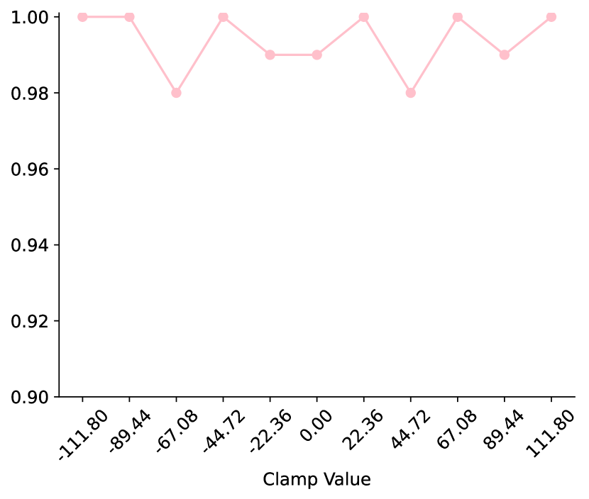
(d)

(e)

(f)

Figure 9: Behavior of the English model under interventions. We examine the causality of features corresponding to other parts of speech: verbs ((a) and (b)), conjunctions ((c) and (d)), and adverbs ((e) and (f)). At each clamp value (x-axis), we plot the distribution of nouns, pronouns, adjectives, verbs, adverbs, and conjunctions.

The results of interventions on various features are shown in Fig. 9. For each part of speech that we show, we follow the same process as in the case of adjectives (Fig. 5):

• determine the maximum value $v_{\text{max}}$ taken by a certain latent;

• pick clamp values at uniform intervals in the range $[-v_{\text{max}},v_{\text{max}}]$; and

• examine (i) the distribution of parts of speech and (ii) the grammaticality of the generations after clamping the latent to each value.

We observe that, similar to the adjectives feature in the main paper (see Fig. 5), the features for other parts of speech do not show causal effects either.

D.3 English: Parts of Speech (with causal loss)

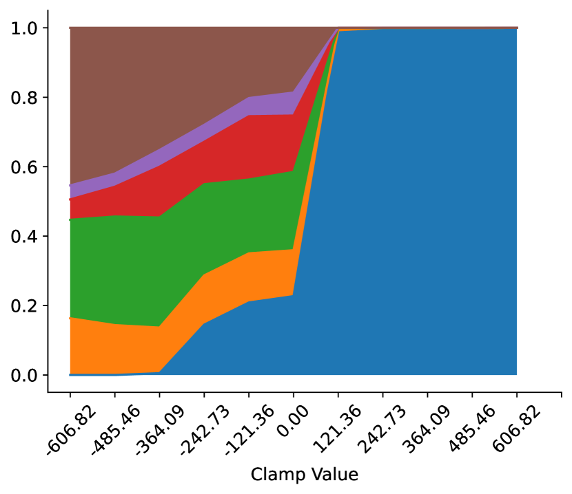
(b)

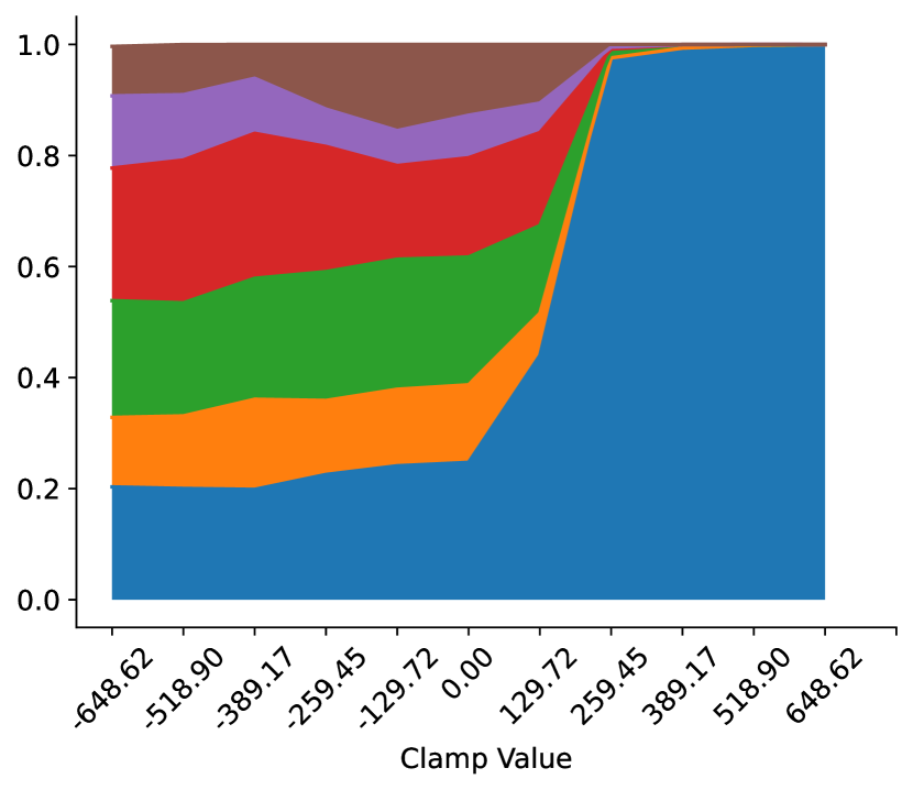
(c)

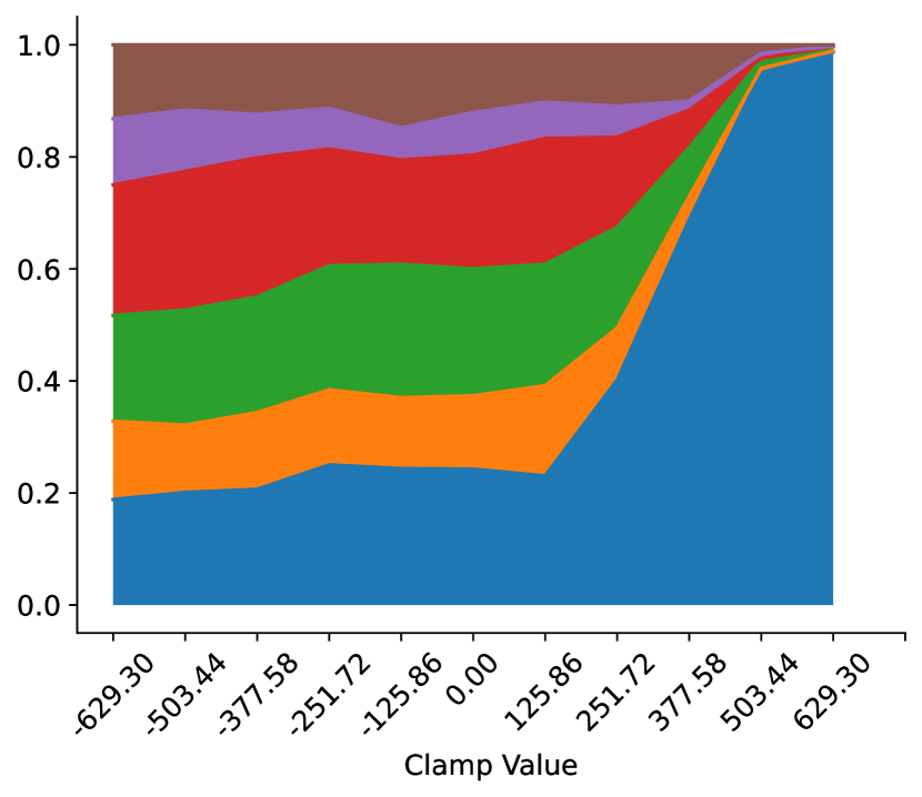
(d)

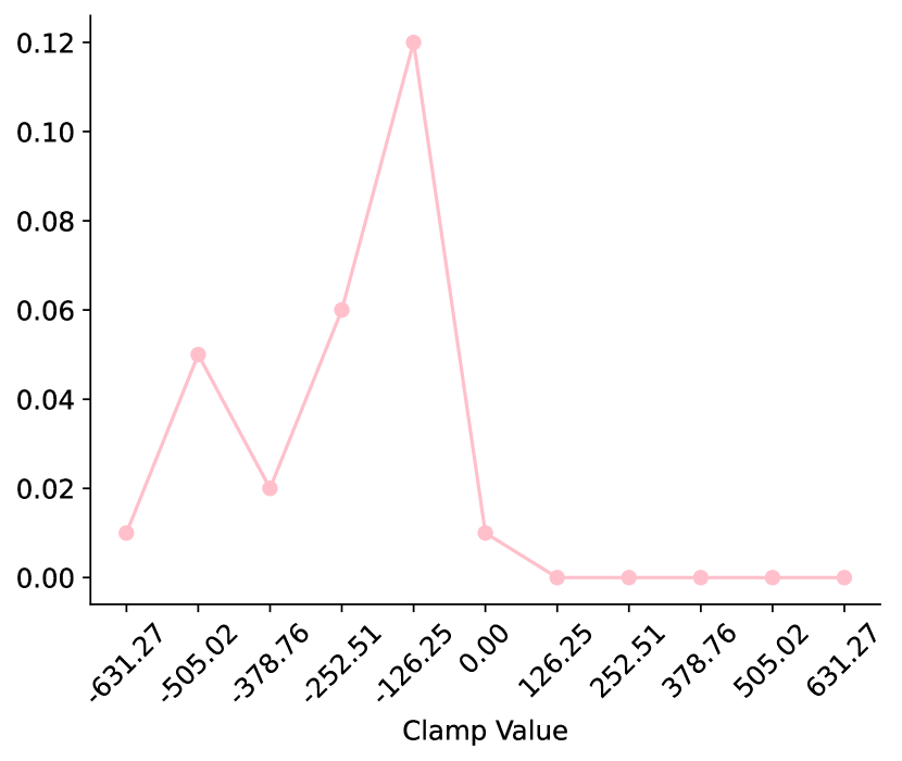
(e) (a) 15/15

(f) (b) 8/15

(g) (c) 4/15

(h) (d) 2/15

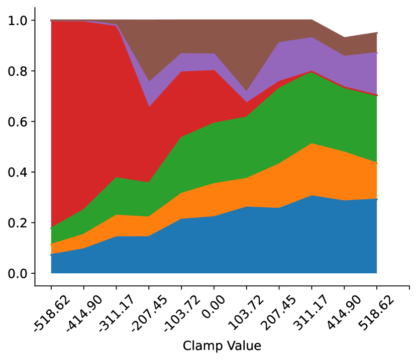
(i)

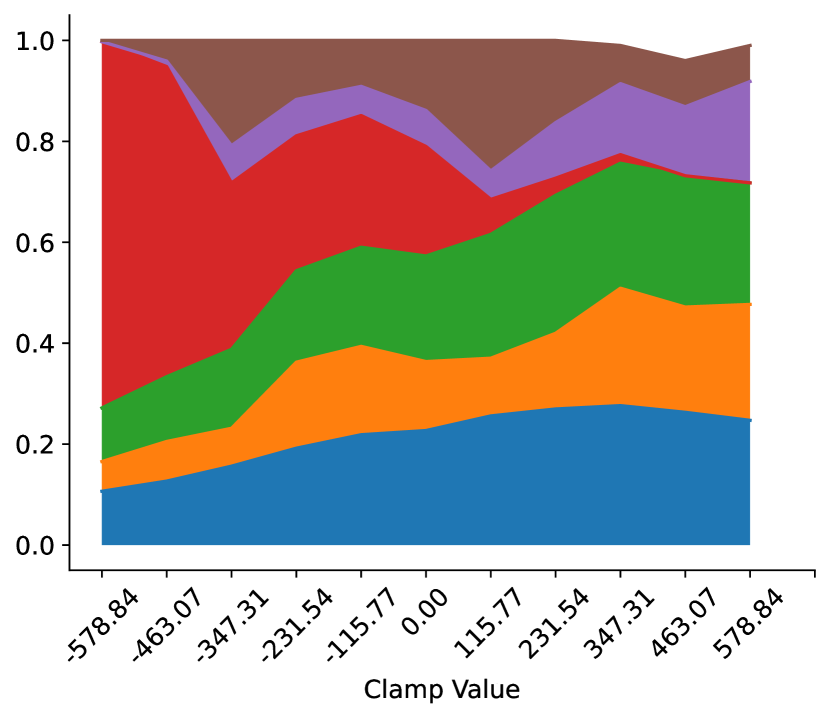
(j)

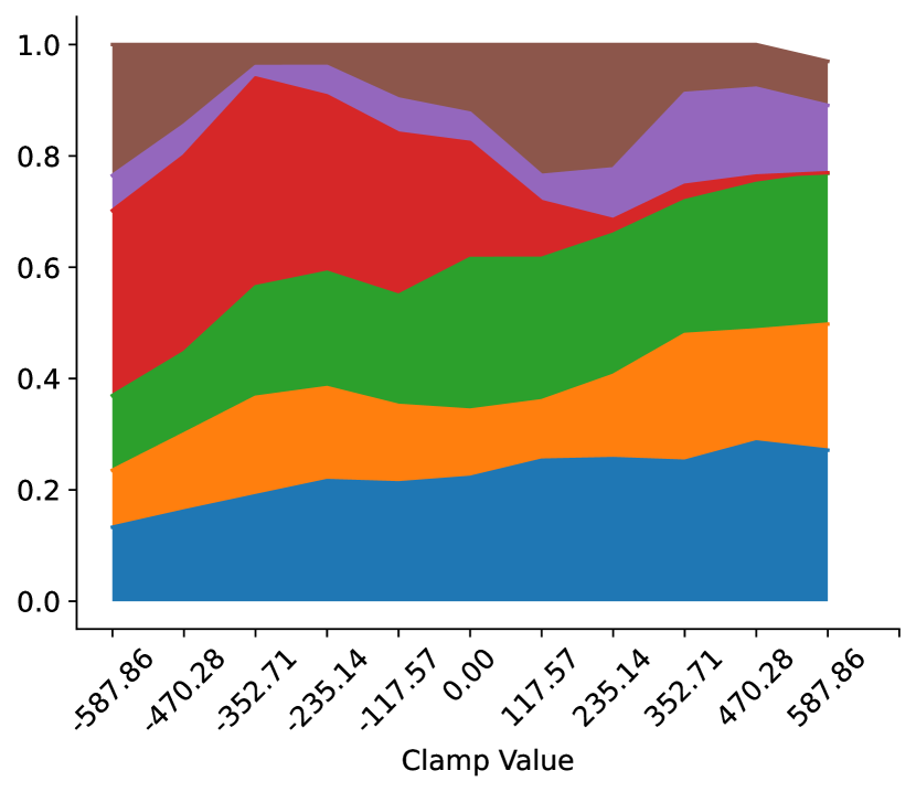
(k)

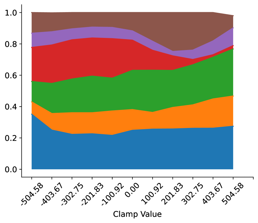
(l)

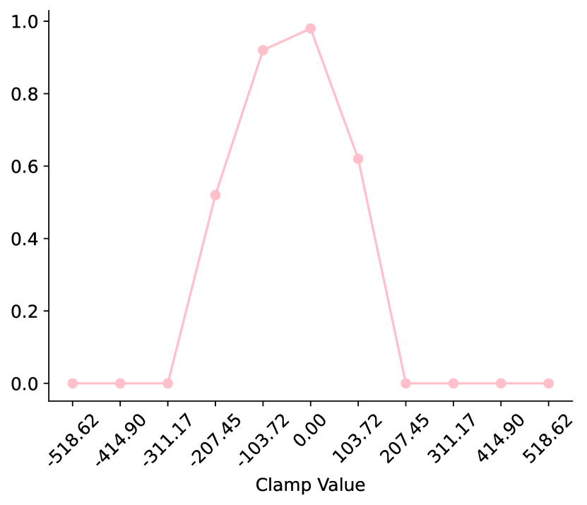
(m) (e) 5/5

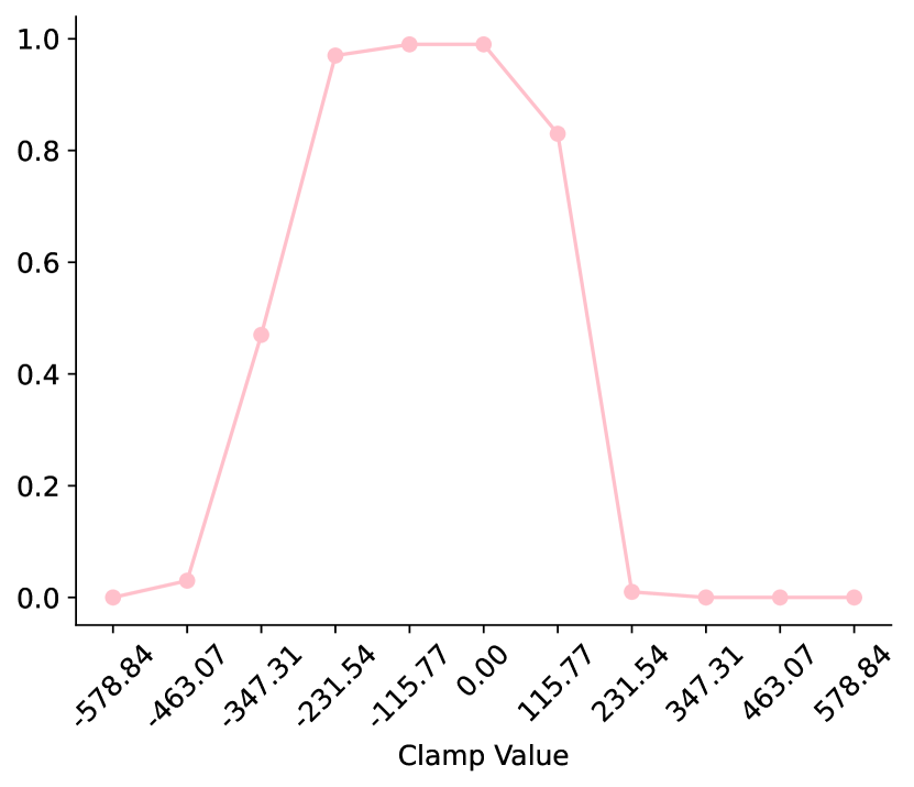
(n) (f) 4/5

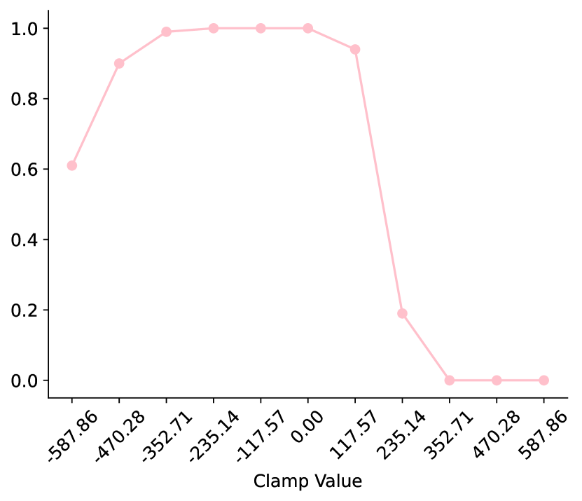
(o) (g) 3/5

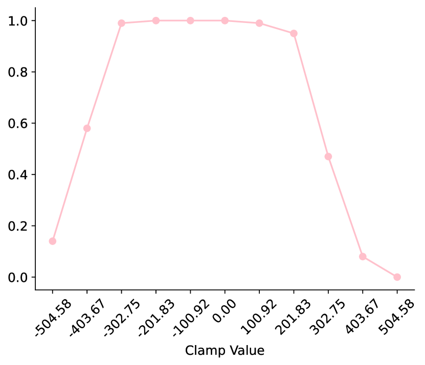
(p) (h) 2/5

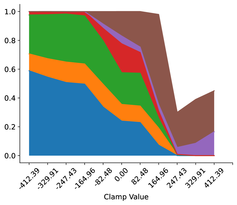
(q)

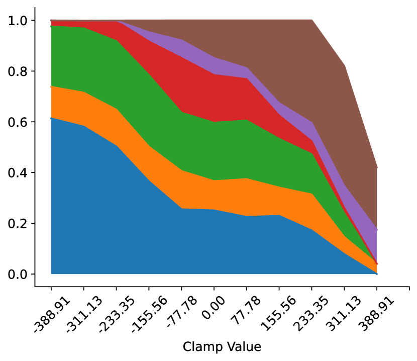
(r)

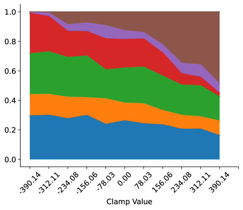
(s)

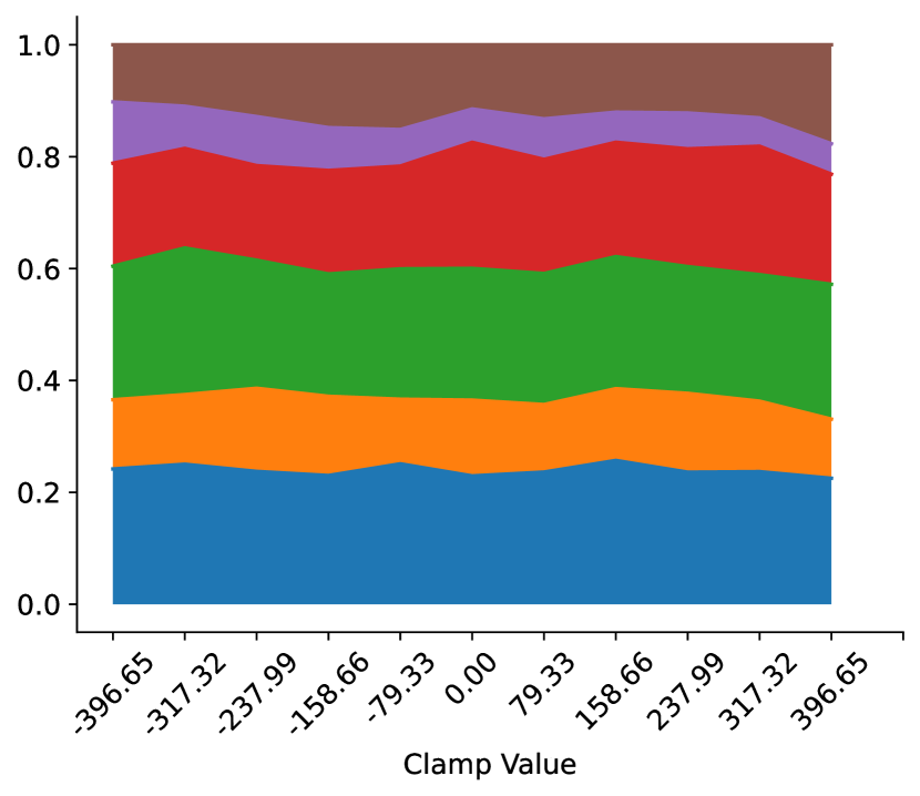
(t)

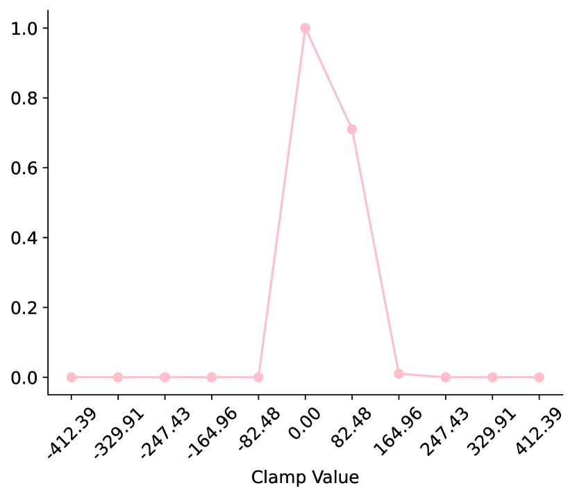
(u) (i) 13/13

(v) (j) 7/13

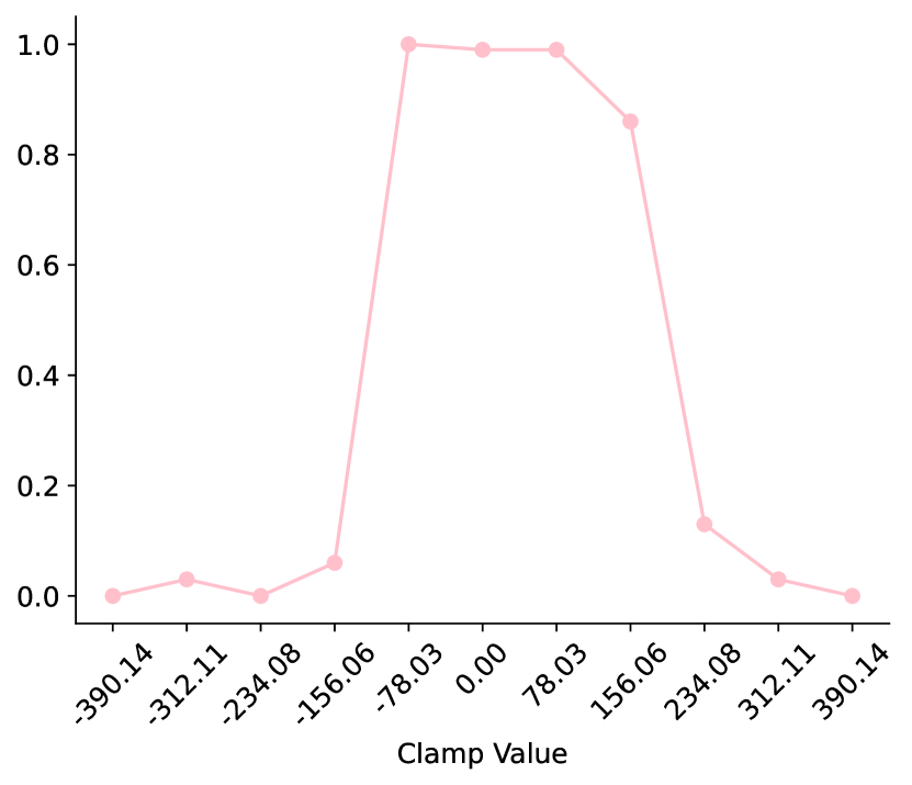
(w) (k) 4/13

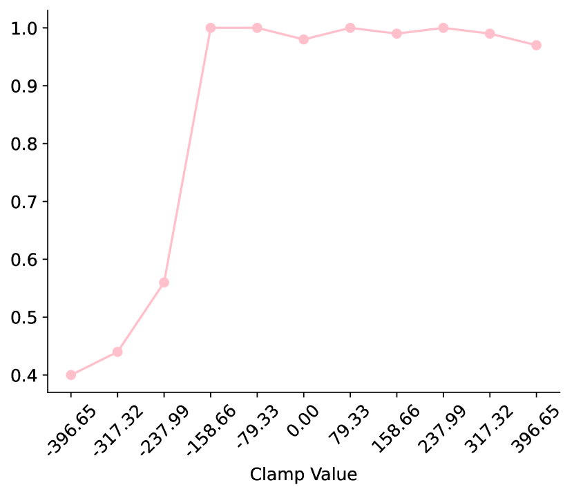
(x) (l) 2/13

Figure 10: Causal effects of adjectives ((a)-(d)), verbs ((e)-(h)), and adverbs ((i)-(l)). The caption of each image describes the number of latents being intervened on. At each clamp value (x-axis), we plot the distribution of nouns, pronouns, adjectives, verbs, adverbs, and conjunctions (top) and the percentage of grammatical generations (bottom).

As mentioned in Sec. 4, our SAEs trained with causal loss demonstrate features correlating with adjectives, verbs, and adverbs. We proceed in essentially the same manner as Sec. D.2 above. As our models, however, identify several features for each part of speech, we show the causal effects of subsets of these feature sets of various sizes, in order to demonstrate the causal effect of the entire set. For instance, if the model has 15 features corresponding to adjectives, we demonstrate causal effects of 15, 8, 4, and 2 features, each of which is obtained by random sampling. We intervene on a set of features in the same way as a single one – by clamping all of the latents to the same value, and resuming the run of the model. The effects of the interventions are shown in Fig. 10.

Applied Corruption	Divergence from Clean Run	Divergence from Corrupted Run
$\Delta x$	$10^{-3}$	$1.37$
$\Delta\operatorname{attn}(x)$	$9.1\cdot 10^{-5}$	$1.38$
$\Delta\operatorname{MLP}(x+\operatorname{attn}(x))$	$1.29$	$6.5\cdot 10^{-3}$
$\Delta_{\text{attn}}\operatorname{MLP}(x+\operatorname{attn}(x))$	$1.44$	$0.04$
$\Delta_{x}\operatorname{MLP}(x+\operatorname{attn}(x))$	$4.8\cdot 10^{-3}$	$1.53$

Table 4: KL divergence between partially corrupted runs, clean runs, and corrupted runs.

Following the logic of Sec. 4.2, we make the following predictions for each part of speech:

• Adjectives. As noted in Sec. 4.1, nouns are the only tokens that can come after adjectives. Therefore we expect the feature correlating with adjectives, if it has a causal effect, to upweight the probability of nouns being predicted.

• Verbs. We have also seen in Sec. 4.1 that any part of speech can follow a verb, except another verb. Thus, we expect the probability of verbs to be reduced by high values of verb-correlated features.

• Adverbs. The grammar (App. B) shows that adverbs can only be followed by conjunctions, more adverbs, or the <EOS> token. We then expect the former two types of tokens to be upweighted, and the other parts of speech dispreferred.

We observe that, in contrast to the features examined in Sec. D.2 above, these features show clear and predictable causal effects.

Appendix E Evidence for Linearity Incentive

Here, we present further evidence for our intuition that the causal loss incentivizes the SAE features to preferentially affect the MLP.

First, we examine the definition of the function $L_{1}$ (the second layer of the model). Ignoring LayerNorm and dropout, this function is simply

$$L_{1}(x)=x+\operatorname{attn}(x)+\operatorname{MLP}\left(x+\operatorname{attn}(x)\right).$$

Thus, when the input $x$ is corrupted to, say $x+\Delta x$, each of these terms lends a corresponding corrupted term the output of $L_{1}$ (and therefore of $g$).

Now, we examine the effect of adding each of these difference terms (separately) to $L_{1}(x)$. If, as we hypothesize, the MLP is the most significantly affected module, then we expect that

$$L_{1}(x) \approx L_{1}(x)+\Delta x$$ (1)

$$L_{1}(x) \approx L_{1}(x)+\Delta\operatorname{attn}(x)$$ (2)

$$L_{1}(x+\Delta x) \approx L_{1}(x)$$

$$+\Delta\operatorname{MLP}(x+\operatorname{attn}(x));$$ (3)

in other words, the effect of the corruption should be replicated by corrupting only the MLP output; and corrupting either of the other two terms should have no effect.

Correspondingly, we can carry this analysis to the input of the MLP module. Here, we expect that the difference in the MLP module’s output can be achieved by corrupting only $x$, and not $\operatorname{attn}(x)$ at all. To make this precise, we define

$$\Delta_{x}\operatorname{MLP}(x +\operatorname{attn}(x))$$

$$=\operatorname{MLP}(x+\Delta x+\operatorname{attn}(x))$$

$$\Delta_{\text{attn}}\operatorname{MLP}(x +\operatorname{attn}(x))$$

$$=\operatorname{MLP}(x+\operatorname{attn}(x+\Delta x)).$$

Then we expect, in line with the previous case, that

$$L_{1}(x) \approx L_{1}(x)$$

$$+\Delta_{\text{attn}}\operatorname{MLP}(x+\operatorname{attn}(x))$$ (4)

$$L_{1}(x+\Delta x) \approx L_{1}(x)$$

$$+\Delta_{x}\operatorname{MLP}(x+\operatorname{attn}(x));$$ (5)

in other words, the corruption of the attention module does not affect the output of the MLP module.
Note that in this setting, the corruption is only applied to the input of the MLP model; the outside $\operatorname{attn}(x)$ term remains as is.

We provide in Tab. 4 the KL divergence between expressions (1), (2), (3), (4) and (5) above, and the distributions corresponding to $L_{1}(x)$ and $L_{1}(x+\Delta x)$. The results are as we expect from the qualitative explanation in Sec. 4. Here, the corruption consists of clamping a feature correlating with adjectives to its maximum value.

Figure	Regularization	pre_bias	Normalization
Fig. 12	$L_{1}$	False	none
Fig. 13	top-$k$	False	none
Fig. 14	$L_{1}$	True	input, decoder
Fig. 15	top-$k$	True	input, decoder
Fig. 16	$L_{1}$	False	input
Fig. 17	top-$k$	False	input
Fig. 18	$L_{1}$	False	input, reconstruction
Fig. 19	top-$k$	False	input, reconstruction

Table 5: Hyperparameter Settings and Corresponding Figures.

It is interesting to note here that we were unable to identify interpretable features in the case of causal SAEs trained on Dyck and Expr models. We explain this, in line with the above, by observing that generation in these languages necessarily requires long-distance memory, in the form of a stack or a counter, which is a function taken up by attention in a transformer model (Bhattamishra et al., 2020). Thus the MLP plays much less of a role in these languages (given the lack of diversity in the vocabulary), and attention is much more important. Since our causal loss avoids identifying features that attention relies on, this explains the lack of features in these two languages.

(a)

(b)

(c)

(a)

Appendix F Power Law in Reconstruction Loss

We noted in Sec. 3 that the top-$k$ regularized SAEs reveal a power law in their reconstruction losses. The trends for various runs are shown in Fig. 11.

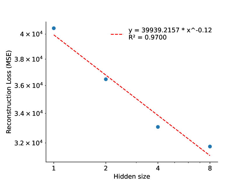
(a)

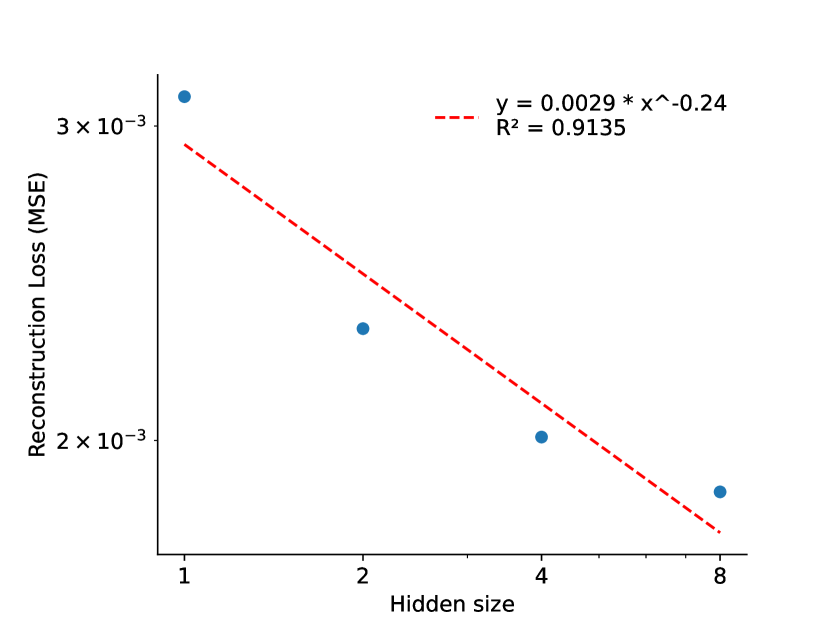
(b)

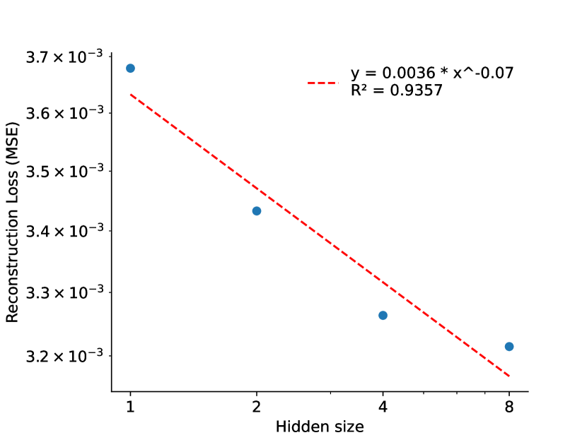
(c)

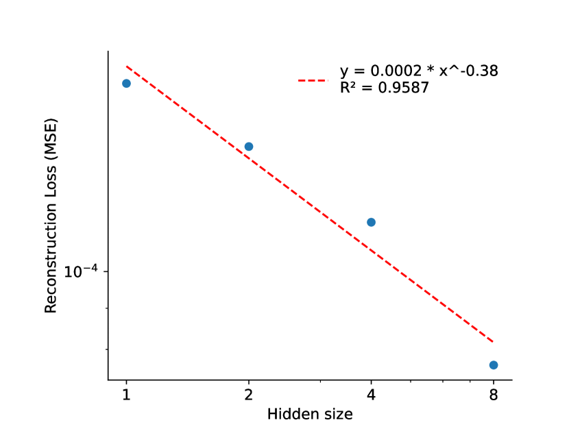
(d)

Figure 11: Scaling law connecting hidden size to reconstruction loss. The power law we identify for each top-$k$ regularized set of autoencoders. The four run sets are (a) without pre_bias or normalization; (b) with pre_bias and normalized inputs and decoder directions; (c) without pre_bias and normalized inputs; and (d) without pre_bias and normalized inputs and reconstructions.

Appendix G Training Details

For both our Transformer and SAE training, we use an online data generation process, that randomly generates a sequence from a given PCFG at every iteration. We use two different datasets for the training and validation in both cases.

Figs. 12 to 19 show the details of the various hyperparameter settings we have considered for SAEs, along with plots of the losses during training. For convenience, we record these details in Tab. 5 as well. Note that, in the case of $L_{1}$-regularized SAEs, the training loss is the sum of the reconstruction loss (the MSE loss between the SAE reconstructions and the inputs) and the regularization loss (the norm of the hidden representation, multiplied by the $L_{1}$ coefficient). The SAEs are trained for 5000 iterations, with losses logged every 25 iterations.

The Transformer models are trained for $7\times 10^{4}$ iterations.

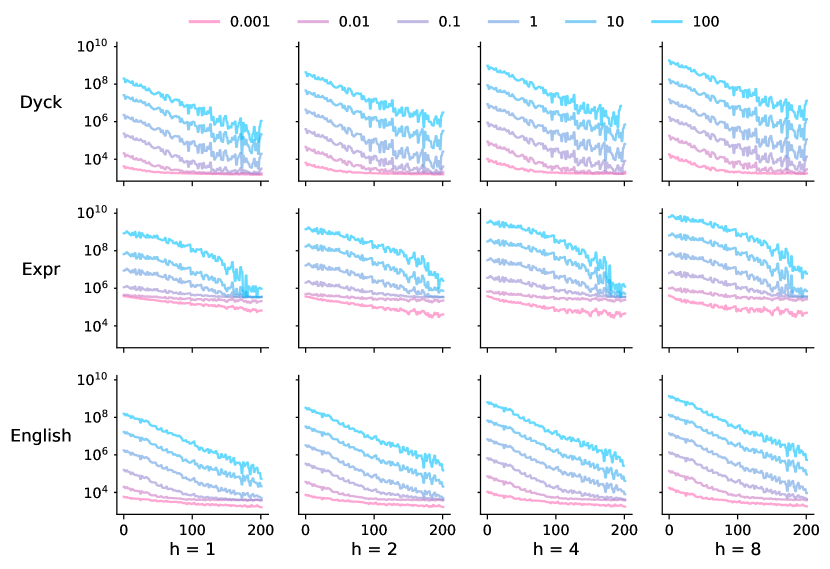
(a) Train Loss (sum of reconstruction and regularization losses)

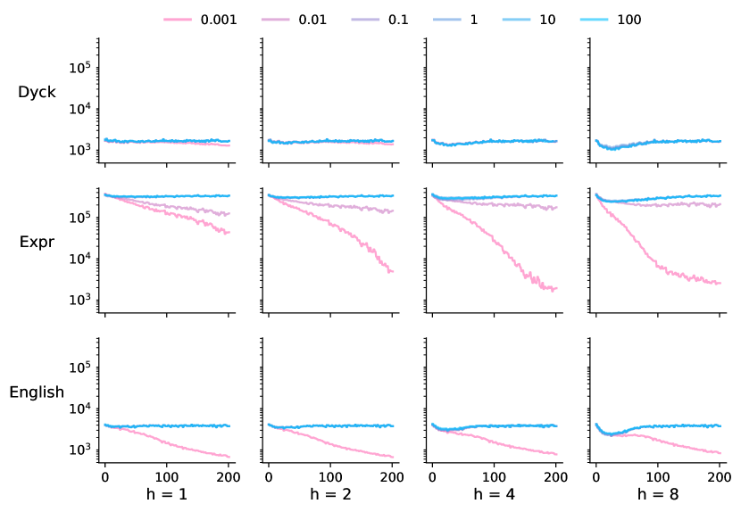
(b) Reconstruction Loss

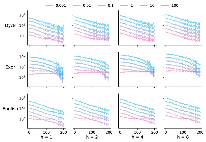
(c) Regularization Loss

Figure 12: $L_{1}$-regularized SAEs, without pre_bias and without normalization.

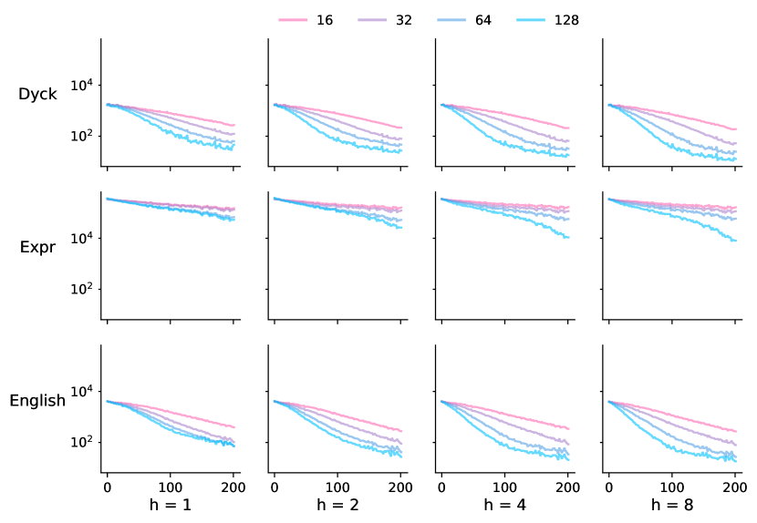
(a) Train Loss (only reconstruction loss)

Figure 13: top-$k$-regularized SAEs, without pre_bias and without normalization.

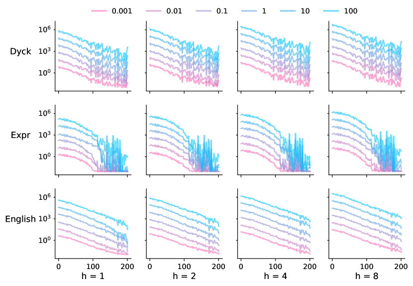
(a) Train Loss (sum of reconstruction and regularization losses)

(b) Reconstruction Loss

(c) Regularization Loss

Figure 14: $L_{1}$-regularized SAEs, with pre_bias and normalized inputs and decoder directions.

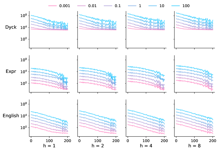
(a) Train Loss (only reconstruction loss)

Figure 15: top-$k$-regularized SAEs, with pre_bias and normalized inputs and decoder directions.

(a) Train Loss (sum of reconstruction and regularization losses)

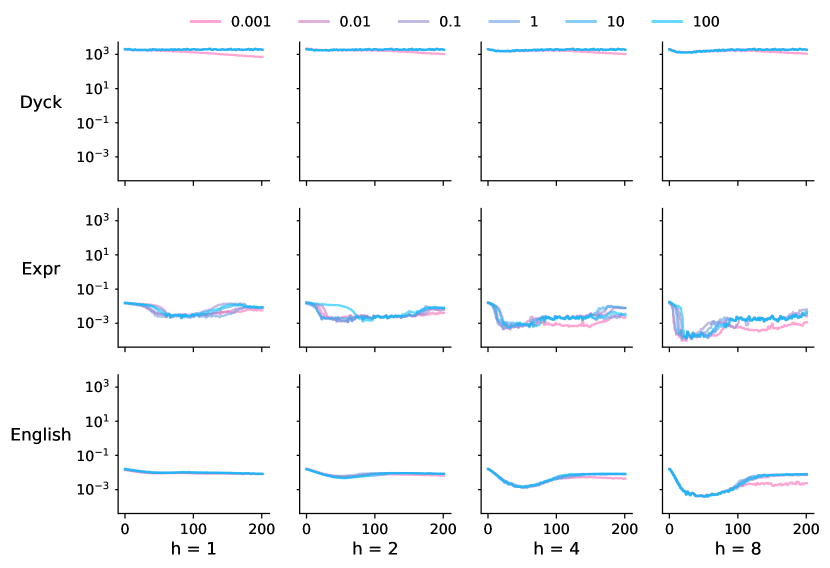
(b) Reconstruction Loss

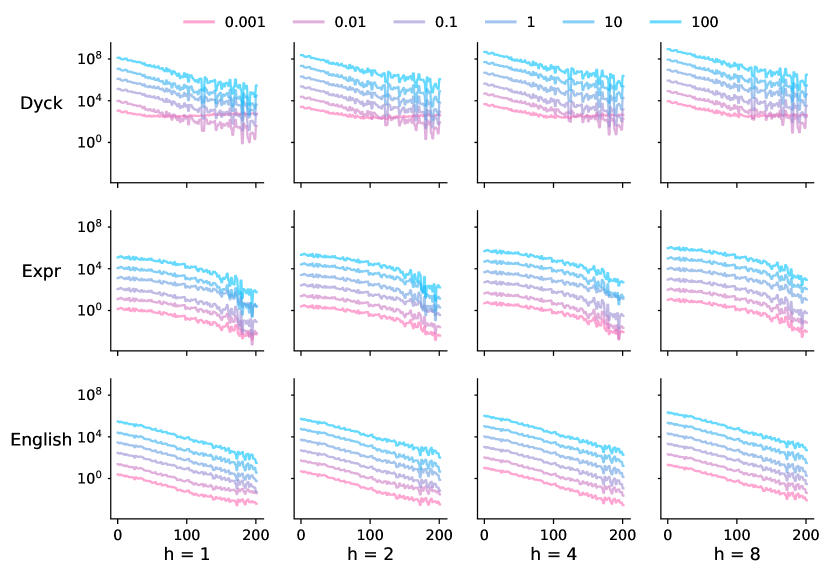
(c) Regularization Loss

Figure 16: $L_{1}$-regularized SAEs, without pre_bias and normalized inputs.

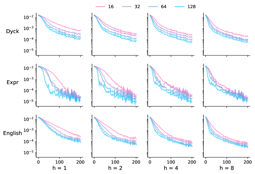
(a) Train Loss (only reconstruction loss)

Figure 17: top-$k$-regularized SAEs, without pre_bias and normalized inputs.

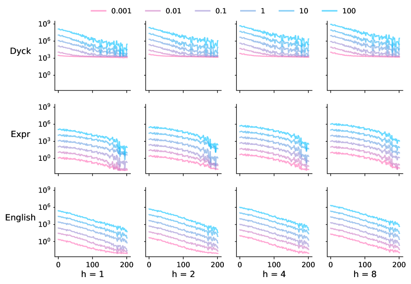
(a) Train Loss (sum of reconstruction and regularization losses)

(b) Reconstruction Loss

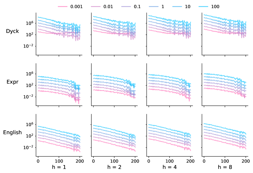
(c) Regularization Loss

Figure 18: $L_{1}$-regularized SAEs, without pre_bias and normalized inputs and reconstructions.

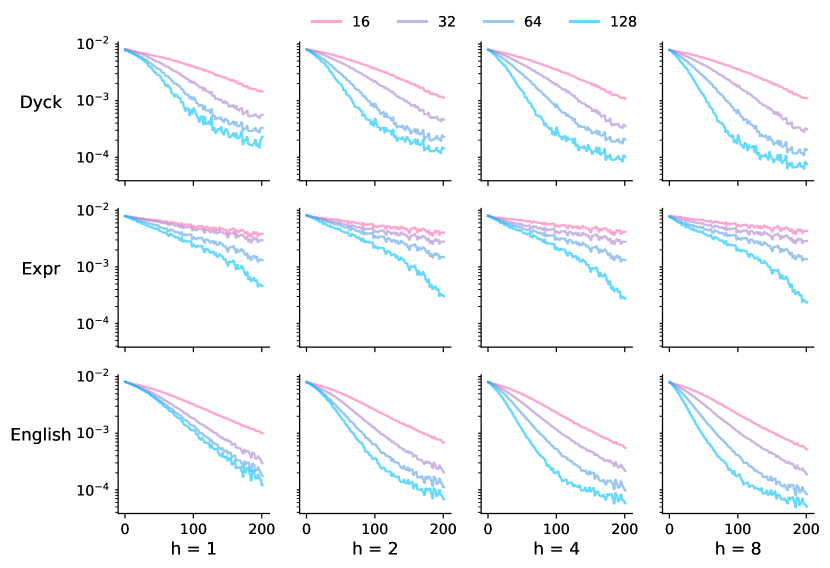
(a) Train Loss (only reconstruction loss)

Figure 19: top-$k$-regularized SAEs, without pre_bias and normalized inputs and reconstructions.

References

- Ahmed et al. (2020) Ossama Ahmed, Frederik Träuble, Anirudh Goyal, Alexander Neitz, Yoshua Bengio, Bernhard Schölkopf, Manuel Wüthrich, and Stefan Bauer. 2020. Causalworld: A robotic manipulation benchmark for causal structure and transfer learning. arXiv preprint arXiv:2010.04296.
- Allen-Zhu and Li (2024) Zeyuan Allen-Zhu and Yuanzhi Li. 2024. Physics of language models: Part 1, learning hierarchical language structures. Preprint, arXiv:2305.13673.
- Bhattamishra et al. (2020) Satwik Bhattamishra, Kabir Ahuja, and Navin Goyal. 2020. On the ability and limitations of transformers to recognize formal languages. arXiv preprint arXiv:2009.11264.
- Braun et al. (2024) Dan Braun, Jordan Taylor, Nicholas Goldowsky-Dill, and Lee Sharkey. 2024. Identifying functionally important features with end-to-end sparse dictionary learning. Preprint, arXiv:2405.12241.
- Brehmer et al. (2022) Johann Brehmer, Pim De Haan, Phillip Lippe, and Taco Cohen. 2022. Weakly supervised causal representation learning. In Advances in Neural Information Processing Systems.
- Bricken et al. (2023) Trenton Bricken, Adly Templeton, Joshua Batson, Brian Chen, Adam Jermyn, Tom Conerly, Nicholas L. Turner, Cem Anil, Carson Denison, Amanda Askell, Robert Lasenby, Yifan Wu, Shauna Kravec, Nicholas Schiefer, Tim Maxwell, Nicholas Joseph, Alex Tamkin, Karina Nguyen, Brayden McLean, Josiah E. Burke, Tristan Hume, Shan Carter, Tom Henighan, and Chris Olah. 2023. Towards monosemanticity: Decomposing language models with dictionary learning. https://transformer-circuits.pub/2023/monosemantic-features.
- Cagnetta et al. (2024) Francesco Cagnetta, Leonardo Petrini, Umberto M Tomasini, Alessandro Favero, and Matthieu Wyart. 2024. How deep neural networks learn compositional data: The random hierarchy model. Physical Review X, 14(3):031001.
- Chaudhary and Geiger (2024a) Maheep Chaudhary and Atticus Geiger. 2024a. Evaluating open-source sparse autoencoders on disentangling factual knowledge in gpt-2 small. arXiv preprint arXiv:2409.04478.
- Chaudhary and Geiger (2024b) Maheep Chaudhary and Atticus Geiger. 2024b. Evaluating open-source sparse autoencoders on disentangling factual knowledge in gpt-2 small. Preprint, arXiv:2409.04478.
- Cunningham et al. (2023) Hoagy Cunningham, Aidan Ewart, Logan Riggs, Robert Huben, and Lee Sharkey. 2023. Sparse autoencoders find highly interpretable features in language models. arXiv preprint arXiv:2309.08600.
- Demircan et al. (2024) Can Demircan, Tankred Saanum, Akshay K. Jagadish, Marcel Binz, and Eric Schulz. 2024. Sparse autoencoders reveal temporal difference learning in large language models. Preprint, arXiv:2410.01280.
- Elhage et al. (2021) Nelson Elhage, Neel Nanda, Catherine Olsson, Tom Henighan, Nicholas Joseph, Ben Mann, Amanda Askell, Yuntao Bai, Anna Chen, Tom Conerly, Nova DasSarma, Dawn Drain, Deep Ganguli, Zac Hatfield-Dodds, Danny Hernandez, Andy Jones, Jackson Kernion, Liane Lovitt, Kamal Ndousse, Dario Amodei, Tom Brown, Jack Clark, Jared Kaplan, Sam McCandlish, and Chris Olah. 2021. A mathematical framework for transformer circuits. Transformer Circuits Thread. Https://transformer-circuits.pub/2021/framework/index.html.
- Engels et al. (2024) Joshua Engels, Isaac Liao, Eric J Michaud, Wes Gurnee, and Max Tegmark. 2024. Not all language model features are linear. arXiv preprint arXiv:2405.14860.
- Gao et al. (2024) Leo Gao, Tom Dupré la Tour, Henk Tillman, Gabriel Goh, Rajan Troll, Alec Radford, Ilya Sutskever, Jan Leike, and Jeffrey Wu. 2024. Scaling and evaluating sparse autoencoders. arXiv preprint arXiv:2406.04093.
- Higgins et al. (2017) Irina Higgins, Loic Matthey, Arka Pal, Christopher Burgess, Xavier Glorot, Matthew Botvinick, Shakir Mohamed, and Alexander Lerchner. 2017. beta-vae: Learning basic visual concepts with a constrained variational framework. International Conference on Learning Representations.
- Hyvarinen and Morioka (2017) Aapo Hyvarinen and Hiroshi Morioka. 2017. Nonlinear ICA of temporally dependent stationary sources. In Artificial Intelligence and Statistics, pages 460–469. PMLR.
- Hyvärinen and Pajunen (1999) Aapo Hyvärinen and Petteri Pajunen. 1999. Nonlinear independent component analysis: Existence and uniqueness results. Neural networks, 12(3):429–439.
- Hyvarinen et al. (2019) Aapo Hyvarinen, Hiroaki Sasaki, and Richard Turner. 2019. Nonlinear ICA using auxiliary variables and generalized contrastive learning. In The 22nd International Conference on Artificial Intelligence and Statistics, pages 859–868. PMLR.
- Karpathy (2022) Andrej Karpathy. 2022. nanogpt. https://github.com/karpathy/nanoGPT.
- Klindt et al. (2020) David Klindt, Lukas Schott, Yash Sharma, Ivan Ustyuzhaninov, Wieland Brendel, Matthias Bethge, and Dylan Paiton. 2020. Towards nonlinear disentanglement in natural data with temporal sparse coding. arXiv preprint arXiv:2007.10930.
- Lachapelle et al. (2023) Sébastien Lachapelle, Tristan Deleu, Divyat Mahajan, Ioannis Mitliagkas, Yoshua Bengio, Simon Lacoste-Julien, and Quentin Bertrand. 2023. Synergies between disentanglement and sparsity: Generalization and identifiability in multi-task learning. In International Conference on Machine Learning, pages 18171–18206. PMLR.
- Lan et al. (2024) Michael Lan, Philip Torr, Austin Meek, Ashkan Khakzar, David Krueger, and Fazl Barez. 2024. Sparse autoencoders reveal universal feature spaces across large language models. Preprint, arXiv:2410.06981.
- Li et al. (2022) Kenneth Li, Aspen K Hopkins, David Bau, Fernanda Viégas, Hanspeter Pfister, and Martin Wattenberg. 2022. Emergent world representations: Exploring a sequence model trained on a synthetic task. arXiv preprint arXiv:2210.13382.
- Li et al. (2024a) Kenneth Li, Oam Patel, Fernanda Viégas, Hanspeter Pfister, and Martin Wattenberg. 2024a. Inference-time intervention: Eliciting truthful answers from a language model. Advances in Neural Information Processing Systems, 36.
- Li et al. (2024b) Zhiyuan Li, Hong Liu, Denny Zhou, and Tengyu Ma. 2024b. Chain of thought empowers transformers to solve inherently serial problems. arXiv preprint arXiv:2402.12875.
- Lieberum et al. (2024) Tom Lieberum, Senthooran Rajamanoharan, Arthur Conmy, Lewis Smith, Nicolas Sonnerat, Vikrant Varma, János Kramár, Anca Dragan, Rohin Shah, and Neel Nanda. 2024. Gemma scope: Open sparse autoencoders everywhere all at once on gemma 2. arXiv preprint arXiv:2408.05147.
- Locatello et al. (2019) Francesco Locatello, Stefan Bauer, Mario Lucic, Gunnar Raetsch, Sylvain Gelly, Bernhard Schölkopf, and Olivier Bachem. 2019. Challenging common assumptions in the unsupervised learning of disentangled representations. In international conference on machine learning, pages 4114–4124. PMLR.
- Locatello et al. (2020) Francesco Locatello, Ben Poole, Gunnar Rätsch, Bernhard Schölkopf, Olivier Bachem, and Michael Tschannen. 2020. Weakly-supervised disentanglement without compromises. In International Conference on Machine Learning, pages 6348–6359. PMLR.
- Lubana et al. (2024) Ekdeep Singh Lubana, Kyogo Kawaguchi, Robert P. Dick, and Hidenori Tanaka. 2024. A percolation model of emergence: Analyzing transformers trained on a formal language. Preprint, arXiv:2408.12578.
- Makelov et al. (2024) Aleksandar Makelov, George Lange, and Neel Nanda. 2024. Towards principled evaluations of sparse autoencoders for interpretability and control. arXiv preprint arXiv:2405.08366.
- Marks et al. (2024) Samuel Marks, Can Rager, Eric J Michaud, Yonatan Belinkov, David Bau, and Aaron Mueller. 2024. Sparse feature circuits: Discovering and editing interpretable causal graphs in language models. arXiv preprint arXiv:2403.19647.
- Nanda et al. (2023) Neel Nanda, Lawrence Chan, Tom Lieberum, Jess Smith, and Jacob Steinhardt. 2023. Progress measures for grokking via mechanistic interpretability. arXiv preprint arXiv:2301.05217.
- Olsson et al. (2022) Catherine Olsson, Nelson Elhage, Neel Nanda, Nicholas Joseph, Nova DasSarma, Tom Henighan, Ben Mann, Amanda Askell, Yuntao Bai, Anna Chen, et al. 2022. In-context learning and induction heads. arXiv preprint arXiv:2209.11895.
- Rajamanoharan et al. (2024) Senthooran Rajamanoharan, Arthur Conmy, Lewis Smith, Tom Lieberum, Vikrant Varma, János Kramár, Rohin Shah, and Neel Nanda. 2024. Improving dictionary learning with gated sparse autoencoders. arXiv preprint arXiv:2404.16014.
- Sepliarskaia et al. (2019) Anna Sepliarskaia, Julia Kiseleva, and Maarten de Rijke. 2019. How to not measure disentanglement. arXiv preprint arXiv:1910.05587.
- Sharkey et al. (2024) Lee Sharkey, Dan Braun, and Beren. 2024. [interim research report] taking features out of superposition with sparse autoencoders. https://www.lesswrong.com/posts/z6QQJbtpkEAX3Aojj/interim-research-report-taking-features-out-of-superposition.
- Shu et al. (2019) Rui Shu, Yining Chen, Abhishek Kumar, Stefano Ermon, and Ben Poole. 2019. Weakly supervised disentanglement with guarantees. arXiv preprint arXiv:1910.09772.
- Sipser (1996) Michael Sipser. 1996. Introduction to the theory of computation. ACM Sigact News, 27(1):27–29.
- Squires et al. (2023) Chandler Squires, Anna Seigal, Salil S Bhate, and Caroline Uhler. 2023. Linear causal disentanglement via interventions. In International Conference on Machine Learning, pages 32540–32560. PMLR.
- Templeton et al. (2024) Adly Templeton, Tom Conerly, Jonathan Marcus, Jack Lindsey, Trenton Bricken, Brian Chen, Adam Pearce, Craig Citro, Emmanuel Ameisen, Andy Jones, Hoagy Cunningham, Nicholas L Turner, Callum McDougall, Monte MacDiarmid, C. Daniel Freeman, Theodore R. Sumers, Edward Rees, Joshua Batson, Adam Jermyn, Shan Carter, Chris Olah, and Tom Henighan. 2024. Scaling monosemanticity: Extracting interpretable features from claude 3 sonnet. Transformer Circuits Thread.
- Träuble et al. (2021) Frederik Träuble, Elliot Creager, Niki Kilbertus, Francesco Locatello, Andrea Dittadi, Anirudh Goyal, Bernhard Schölkopf, and Stefan Bauer. 2021. On disentangled representations learned from correlated data. In International conference on machine learning, pages 10401–10412. PMLR.
- Verma et al. (2019) Vikas Verma, Alex Lamb, Christopher Beckham, Amir Najafi, Ioannis Mitliagkas, David Lopez-Paz, and Yoshua Bengio. 2019. Manifold mixup: Better representations by interpolating hidden states. In International conference on machine learning, pages 6438–6447. PMLR.
- Wang et al. (2022) Kevin Wang, Alexandre Variengien, Arthur Conmy, Buck Shlegeris, and Jacob Steinhardt. 2022. Interpretability in the wild: a circuit for indirect object identification in gpt-2 small. arXiv preprint arXiv:2211.00593.
- Wen et al. (2024) Kaiyue Wen, Yuchen Li, Bingbin Liu, and Andrej Risteski. 2024. Transformers are uninterpretable with myopic methods: a case study with bounded dyck grammars. Advances in Neural Information Processing Systems, 36.