Abstract

We address the challenge of causal discovery in structural equation models with additive noise without imposing additional assumptions on the underlying data-generating process. We introduce local search in additive noise model (LoSAM), which generalizes an existing nonlinear method that leverages local causal substructures to the general additive noise setting, allowing for both linear and nonlinear causal mechanisms. We show that LoSAM achieves polynomial runtime, and improves runtime and efficiency by exploiting new substructures to minimize the conditioning set at each step. Further, we introduce a variant of LoSAM, LoSAM-UC, that is robust to unmeasured confounding among roots, a property that is often not satisfied by functional-causal-model-based methods. We numerically demonstrate the utility of LoSAM, showing that it outperforms existing benchmarks.

1 Introduction

Causal discovery algorithms aim to learn the causal structure of data-generating processes (DGPs) from observational data by representing them as causal graphical models. These methods have fundamental applications in science, healthcare, and economics, enabling important downstream inference tasks such as causal effect estimation (Hoyer et al.,, 2008; Cheng et al.,, 2023; Shah et al.,, 2024). Traditional discovery methods can generally be classified as either constraint-based, leveraging conditional independence tests to identify causal relationships, or scoring-based, searching over the space of possible causal models and selecting the one that maximizes a goodness-of-fit measure (Glymour et al.,, 2019). While these nonparametric discovery methods have general applicability, they often suffer from worst-case exponential time complexity (Spirtes,, 2001), are limited to learning Markov equivalence classes (MEC) rather than unique directed acyclic graphs (DAGs) (Montagna et al., 2023a, ), and have poor sample efficiency, displaying finite sample failure modes even with reasonably large sample sizes (Maasch et al.,, 2024).

To enable worst-case polynomial time discovery of the unique DAG, various methods based on functional-causal-models (FCM) have been proposed (Zhang and Hyvarinen,, 2009). FCMs impose parametric assumptions on the functional form of the DGP to aid the discovery process. The additive noise model (ANM) is a popular modeling approach, where the causal parents of a variable are assumed to be statistically independent of its noise term; causal relationships are identified when a variable of interest is regressed against its hypothesized parent set, and an independent residual is recovered (Peters et al.,, 2014). However, most popular FCM-based methods either impose stronger assumptions over the functional form such as linearity (Shimizu et al.,, 2011), or suffer in sample complexity due to the use of high-dimensional nonparametric regressions (Peters et al.,, 2014; Montagna et al., 2023b, ).

Contributions  We propose a novel global causal discovery approach to graph learning in FCM that builds upon the method NHTS, proposed by Hiremath et al., (2024). NHTS leverages causal substructures in a local search approach to boost sample and computational efficiency, assuming nonlinear data-generating mechanisms. We depart from NHTS by 1) characterizing conditions that allow us to handle a more general class of causal models, including ANMs with both linear and nonlinear relations, and 2) leveraging proxy variables for discovery in models with latent unmeasured confounders. Further, we identify new local causal substructures that allow to us improve both sample and computational efficiency. Our approach learns the DAG from roots to leaves, leveraging the identification of roots to reduce the size of conditioning sets used in nonparametric regressions, and developing a continuous measure of residual dependence to improve algorithm stability. We summarize our contributions below:

• We introduce LoSAM, a novel topological ordering algorithm, designed for ANMs with both linear and nonlinear functions.

• We introduce a variant of LoSAM, LoSAM-UC, that is robust to unmeasured confounders between root vertices in ANMs.

• We evaluate LoSAM on synthetic data, outperforming baselines with higher accuracy and faster runtime.

Related Works  Traditional constraint-based methods include PC (Spirtes et al.,, 2000) and FCI (Spirtes,, 2001), while GES (Chickering,, 2002) and GRaSP (Lam et al.,, 2022) are popular scoring-based methods; these methods recover an equivalence class. Our work is most closely related to various FCM-based methods, each of which makes different parametric assumptions to recover the unique DAG. Early approaches such as ICA-LiNGAM (Shimizu et al.,, 2006) and DirectLiNGAM (Shimizu et al.,, 2011) tackle the simplest case of DAGs generated by linear functions and non-Gaussian noise terms. CAM (Bühlmann et al.,, 2014) assumes a generalized additive noise model and Gaussian noise, whereas RESIT (Peters et al.,, 2014), NoGAM (Montagna et al., 2023b, ), and NHTS (Hiremath et al.,, 2024) handle the more general class of nonlinear ANMs with arbitrary noise distributions.

Organization  We introduce preliminaries in Section 2, and the fully observed setting in Section 3. We establish various ancestor-descendant local causal substructures, introducing a topological sorting algorithm LoSAM. Next, we extend our method to the partially observed setting in Section 4 by leveraging proxy variables, developing LoSAM-UC. We test LoSAM in synthetic experiments and conclude in Section 5.

2 Preliminaries

An structural equation model (SEM) is represented by a DAG, denoted as $G=(V,E)$ on $|V|=d$ vertices, where $E$ represents directed edges. An edge $x_{i}\rightarrow x_{j}\in E$ iff (if and only if) $x_{i}$ has a direct causal influence on $x_{j}$. We define four pairwise relationships between vertices: 1) $\text{Ch}(x_{i})$ denotes the children of $x_{i}$ such that $x_{j}\in\text{Ch}(x_{i})$ iff $x_{i}\to x_{j}$, 2) $\text{Pa}(x_{i})$ denotes the parents of $x_{i}$ such that $x_{j}\in\text{Pa}(x_{i})$ iff $x_{j}\to x_{i}$, 3) $\text{An}(x_{i})$ denotes the ancestors of $x_{i}$ such that $x_{j}\in\text{An}(x_{i})$ iff there exists a directed path $x_{j}\dashrightarrow x_{i}$, 4) $\text{De}(x_{i})$ denotes the descendants of $x_{i}$ such that $x_{j}\in\text{De}(x_{i})$ iff there exists a directed path $x_{i}\dashrightarrow x_{j}$. We consider four vertex categories based on the totality of their pairwise relationships: 1) $x_{i}$ is a root iff $\text{Pa}(x_{i})=\emptyset$, 2) a leaf iff $\text{Ch}(x_{i})=\emptyset$, 3) an isolated vertex iff $x_{i}$ is both a root and a leaf, and 4) an intermediate vertex otherwise. We also classify vertices in terms of their triadic relationships: $x_{i}$ is a confounder of $x_{j}$ and $x_{k}$ if $x_{i}\in\text{An}(x_{j})\cap\text{An}(x_{k})$, or a mediator of $x_{j}$ to $x_{k}$ if $x_{i}\in\text{De}(x_{j})\cap\text{An}(x_{k})$.

Definition 2.1 (Topological Ordering).

Consider a DAG denoted as $G=(V,E)$. We say that a mapping $\pi:V\rightarrow\{0,1,\ldots,|V|\}$ is a linear topological sort iff $\;\forall x_{j}\in V$, whenever $x_{i}\in\text{Pa}(x_{j})$, $x_{i}$ appears before $x_{j}$ in the sort $\pi$, i.e., $\pi(x_{i})<\pi(x_{j})$.

Definition 2.2 (ANMs, Hoyer and Hyttinen, 2009).

Additive noise models are a general class of SEMs with

$$x_{i}=f_{i}(\text{Pa}(x_{i}))+\varepsilon_{i}$$ (1)

$\forall x_{i}\in V$, where $f_{i}$’s are arbitrary functions and $\varepsilon_{i}$’s are independent arbitrary noise distributions.

Definition 2.2 implicitly assumes the Causal Markov condition and acyclicity; we further assume faithfulness (Spirtes and Zhang,, 2016), as well as the unique identifiability of the ANM (see Appendix C for details).

3 Fully Observed Model

FCM-based approaches that leverage the additive noise assumption often decompose the graph learning problem into two phases: 1) inferring a causal ordering of the variables (topological ordering), and 2) identifying edges consistent with the causal ordering (edge pruning). Recently, Hiremath et al., (2024) leveraged local causal substructures to develop sample-efficient topological sorting algorithms and a nonparametric edge-pruning method; however, their sorting algorithms (LHTS, NHTS) were designed only to handle ANMs with either linear or nonlinear causal mechanisms. Mixed causal mechanisms pose a challenge because the conditions required to recover an independent residual (and thereby identify a causal relationship) vary based on the underlying functional relationships. Hiremath et al., (2024) show that in linear models specific ancestor-descendant pairs yield independent residuals, whereas the same test may yield dependent residuals when the mechanism is nonlinear.

To overcome the need to constrain the functional form, in this section we propose LoSAM, a novel topological ordering algorithm that generalizes NHTS to handle ANMs with both linear and nonlinear mechanisms, while improving sample and computational efficiency. Similar to NHTS, LoSAM follows a two-step procedure: 1) identifying the root vertices (Algorithm 1, Section 3.1), and 2) leveraging root vertices to identify the rest of the topological sort (Algorithm 2, Section 3.2). In Section 3.3, we build upon the above subroutines and introduce the full procedure of LoSAM.

3.1 Root Finding

To develop a subroutine for identifying roots in both linear and nonlinear causal mechanisms, we must identify properties that are unique to roots. We will establish a novel set of local causal structures where roots behave distinctly from non-roots, regardless of their functional relationship. Starting with the entire vertex set $V$, we iteratively prune away non-roots by leveraging these asymmetric properties, yielding only the roots.

We first note that non-roots can be partitioned into two distinct categories: those descending from a single root and those descending from multiple roots.

Definition 3.1 (Single Root Descendant).

A vertex $x_{i}\in V$ is a single root descendant (SRD) iff $\exists$ only one root $x_{j}$, such that $x_{j}\in\text{An}(x_{i})$.

Definition 3.2 (Multi Root Descendant).

A vertex $x_{i}\in V$ is a multi root descendant (MRD) iff $\exists$ at least two roots $x_{j},x_{k}$ such that $x_{j},x_{k}\in\text{An}(x_{i})$.

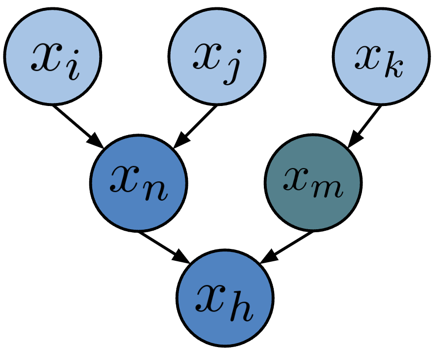
Figure 1: Exemplary DAG where $x_{i},x_{j},x_{k}$ are roots, $x_{m}$ is an SRD, and $x_{n},x_{h}$ are MRDs that induce VPs between $x_{i},x_{j}$.

Visually, we see this division of non-root vertices into SRDs and MRDs in Figure 1. For any MRD $x_{i}\in V$, we observe that $x_{i}$ forms a ‘v’ with any two of its root ancestors. We define this ancestor-descendant local substructure as a v-pattern (VP), and give a characterization based on marginal dependence constraints:

Definition 3.3 (VP).

We say that a vertex $x_{i}$ induces a v-pattern iff there exist two vertices $x_{j},x_{k}\in V$ such that $x_{i}\not\!\perp\!\!\!\perp x_{j},x_{i}\not\!\perp\!\!\!\perp x_{k},$ $x_{j}\perp\!\!\!\perp x_{k}$.

Definition 3.3 generalizes the notion of ‘v-structure’ (Spirtes et al.,, 2000) to a ancestral-descendant relationship. A v-structure can be thought of as a special case of a VP, where the inducing vertex is a child of the two other vertices. Next, in Lemma 3.1, we leverage VP to distinguish MRDs from SRDs and roots.

Lemma 3.1 (MRD Induces VP).

A vertex $x_{i}$ induces a VP iff $x_{i}$ is an MRD.

The proof of Lemma 3.1 (Appendix D.1) relies on the fact that all vertices in $V$ are partitioned into roots, SRDs, and MRDs. We further observe that 1) an MRD induces a VP because roots are all independent of each other, and 2) an SRD or a root does not induce VP.

Lemma 3.1 implies that by checking whether a vertex induces a VP between any two vertices in $V$, we can identify and prune MRDs from $V$, resulting in a subset $V^{\prime}\subset V$ containing only SRDs and roots. It remains to prune SRDs from $V^{\prime}$.

Next, in Lemma 3.2 (proof in Appendix D.2), we show that a root with no SRDs can be identified by testing for independence from the other variables in $V^{\prime}$:

Lemma 3.2 (Root with No SRDs).

For any $x_{i}\in V^{\prime}$, if $x_{i}\perp\!\!\!\perp x_{j}\;\forall x_{j}\in V^{\prime}\setminus\{x_{i}\}$, $x_{i}$ is a root with no SRDs.

Let $V^{\prime\prime}$ be the remaining vertices after identifying roots with no SRDs using Lemma 3.2. This set consists of roots with at least one SRD, along with the SRDs themselves. Like NTHS, we follow a two-step procedure to first recover a subset of roots through nonparametric regression, followed by pruning the remaining non-roots using conditional independence tests. To identify the children of the roots, NTHS leverages pairwise nonparametric regression, which yields an independent residual when a non-root is a child of the root and causal mechanisms are nonlinear. However, when the mechanism is linear, this procedure can also identify non-roots that are descendants of the root. We formally state the outcome of a nonparametric regression residual test below, considering both linear and nonlinear mechanisms.

Definition 3.4 (Ancestor-Descendant Test).

Let $x_{i},x_{j}\in V^{\prime\prime}$, and let $r_{ij}$ be the residual of $x_{j}$ nonparametrically regressed on $x_{i}$. Then, $x_{i}$ is identified as $\in\text{An}(x_{j})$ iff: 1) $x_{i}\perp\!\!\!\perp r_{ij}$, and 2) $x_{j}\not\!\perp\!\!\!\perp r_{ij}$.

Next, using the Ancestor-Descendant test in Definition 3.4, Lemma 3.3 establishes that the subset $W$ of $V^{\prime\prime}$ contains all the roots, which can be distinguished from non-roots within $W$:

Lemma 3.3 (Root ID).

Let $W$ be a subset of $V^{\prime\prime}$ such that $\forall x_{i}\in W$, 1) $\exists x_{j}\in V$ such that $x_{i}$ is identified as $\in\text{An}(x_{j})$, and 2) $\nexists x_{k}\in V$ such that $x_{k}$ is identified as $\in\text{An}(x_{i})$. Then $W$ contains all roots in $V^{\prime\prime}$.

Further, a vertex $x_{i}\in W$ is a root iff $\forall x_{j}\in W\setminus\{x_{i}\}$ with $x_{j}\not\!\perp\!\!\!\perp x_{i}$, there exists $x_{k}\in V^{\prime\prime}$ such that 1) $x_{i}$ is identified as $\in\text{An}(x_{k})$ and 2) $x_{i}$ does not d-separate $x_{k}$ and $x_{j}$, i.e., $x_{k}\not\!\perp\!\!\!\perp x_{j}|x_{i}$.

Note that $W$ will contain any SRDs that pass the Ancestor-Descendant Test; one such subcase occurs when an SRD has a child, and is its only parent. To distinguish the roots from these SRDs, the proof of Lemma 3.3 (Appendix D.3) relies on the intuition that, for any root vertex $x_{i}$ and SRD $x_{j}\in\text{De}(x_{i})$, there exists a child of $x_{i},x_{k}\in\text{Ch}(x_{i})$, such that $x_{k}$ is a mediator of $x_{i}$ to $x_{j}$. This implies that $x_{i}$ satisfies both conditions of Lemma 3.3. Note that any child $x_{k}$ of a root $x_{i}$ cannot be included in $W$, as the Ancestor-Descendant Test will always identify $x_{i}\in\text{An}(x_{k})$. On the other hand, SRDs in $W$ will fail to satisfy the second condition in Lemma 3.3: this asymmetry allows SRDs to be pruned.

Algorithm 1 outlines our root-finding procedure. In Stage 1, we run marginal independence tests between all vertices, leveraging Lemmas 3.1 and 3.2 to prune MRDs and roots with no SRDs, leaving SRDs and their root ancestors. In Stage 2, we run pairwise nonparametric regressions and independence tests on regressors and residuals to obtain the root superset $W$. We then apply Lemma 3.3, using conditional independence tests to identify the remaining roots. We show the asymptotic correctness of Algorithm 1 in Proposition 3.5 (proof in Appendix E.1):

1:Input: vertices $x_{1},\ldots,x_{d}\in V$.

2:Initialize: root set $RT$, root superset $W$.

3:Stage 1: Prune MRDs, Obtain Some Roots

4:Run pairwise $\perp\!\!\!\perp$ tests between each pair of vertices $x_{i},x_{j}\in V$ and remove all vertices that induce a VP (MRDs) from $V$ to obtain $V^{\prime}$.

5:Add any vertex $x_{i}\in V^{\prime}$ to $RT$ if $x_{i}\perp\!\!\!\perp x_{j}\forall x_{j}\in V^{\prime}\setminus{\{x_{i}\}}$, and remove all $x_{i}$ from $V^{\prime}$ to obtain $V^{\prime\prime}$.

6:Stage 2: Prune SRDs, Obtain Leftover Roots

7:Run pairwise nonparametric regression between $x_{i},x_{j}\in V^{\prime\prime}$; if $\exists x_{l}$ such that $x_{k}\in V^{\prime\prime}$ is identified as $\in\text{An}(x_{j})$, and there does not exist $x_{h}$ such that $x_{h}$ is identified $\in\text{An}(x_{k})$, add $x_{k}$ to $W$.

8:For $x_{i}\in W$, if $\forall x_{j}\in W\setminus{\{x_{i}\}}$ such that $x_{j}\not\!\perp\!\!\!\perp x_{i}$, $\exists x_{k}\in V^{\prime\prime}$ such that $x_{i}$ is identified as $\in\text{An}(x_{k})$ and $x_{k}\not\!\perp\!\!\!\perp x_{j}|x_{i}$, add $x_{i}$ to $RT$.

9:return $RT$.

Algorithm 1 Root Finder

Proposition 3.5.

Given the vertices of a DAG $G$ generated by an ANM, Algorithm 1 asymptotically returns the correct set of root vertices.

To our knowledge, our approach is the first to identify root vertices in ANMs without requiring any multivariate nonparametric regressions. In contrast, high-dimensional regressions are often a bottleneck for sample and computational efficiency (Peters et al.,, 2014), which limits many FCM-based methods from recovering the true topological sort from finite samples, despite asymptotic guarantees. In Theorem 3.6 (proof in Appx F.1), we formally show the reduction in the size of the conditioning sets used in Alg 1 compared to NHTS:

Theorem 3.6.

Given a DAG $G=(V,E)$ under an ANM, let $M\subseteq V$ and $R\subseteq V$ be the sets of MRDs and roots in $G$, respectively. Let $c^{\mathrm{Alg1}}_{\mathrm{max}}$ be the maximum conditioning set size in nonparametric regressions in Algorithm 1, and similarly, $c^{\mathrm{NHTS}}_{\mathrm{max}}$ for the root identification step in NHTS. Then, $c^{\mathrm{Alg1}}_{\mathrm{max}}=1$, and $c^{\mathrm{NHTS}}_{\mathrm{max}}$ = $\max_{x_{i}\in M}(\text{An}(x_{i})\cap R,0)$. This implies that $c^{\mathrm{Alg1}}_{\mathrm{max}}\leq c^{\mathrm{NHTS}}_{\mathrm{max}}$, and when $M\neq\emptyset$, $c^{\mathrm{Alg1}}_{\mathrm{max}}<c^{\mathrm{NHTS}}_{\mathrm{max}}$.

By leveraging the existence of VPs to prune MRDs, we limit conditioning sets used in nonparametric regressions in Algorithm 1 to a maximum size of one, improving sample efficiency and achieving faster runtime compared to the corresponding step in NHTS.

3.2 Sort Finding

After obtaining the set of roots, we develop Algorithm 2, which sorts the remaining non-roots into a topological ordering $\pi$. Similar to NHTS, we start by adding roots to $\pi$ in any order (because roots share no edges), leaving the unsorted vertices $U=V\setminus{\pi}$. We follow an iterative procedure by removing one vertex at a time from $U$ and adding it to $\pi$, ensuring the resulting $\pi$ is valid (Definition 2.1). In each iteration, we identify a valid candidate (VC) as illustrated in Figure 2:

Definition 3.7 (VC).

A vertex $x_{i}\in U$ is a valid candidate iff $\text{Pa}(x_{i})\cap U=\emptyset$.

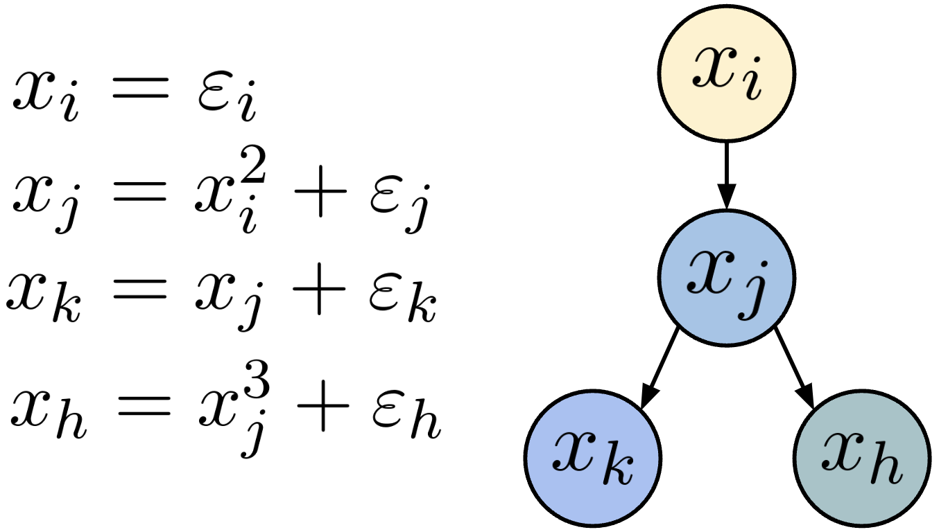
Figure 2: Exemplary DAG, where $x_{i}$ has been sorted into $\pi$, $x_{j}$ is a VC, $x_{k}$ is a LD, $x_{h}$ is a ND.

We proceed by first partitioning non-VC vertices in $U$ into different categories, relying on novel local causal substructures. We then leverage asymmetric properties to prune non-VCs from $U$, allowing the identification of a VC at each iteration. Before we introduce our substructures, we first note that the sort identification step in NHTS may incorrectly sort ANMs with both linear and nonlinear mechanisms.

Each iteration of NHTS’s sorting procedure consists of two stages: first, each vertex $x_{i}\in U$ is nonparametrically regressed onto the sorted vertices in $\pi$, producing a set of residuals $U_{E}$ (where $e_{i}\in U_{E}$ is the residual of $x_{i}$ regressed onto vertices in $\pi$). Second, independence tests are run between each residual $e_{i}$ and every vertex in $\pi$, and any vertex whose residual is independent of all vertices in $\pi$ is selected from $U$ and added to $\pi$.

This procedure exploits the fact that, for each non-VC $x_{i}\in U$ in a nonlinear ANM, there exists a mediator $x_{j}\in\text{An}(x_{i})\cap U$ between vertices in $\pi$ to $x_{i}$ such that $x_{i}$ is a nonlinear function of $x_{j}$. In Definition 3.8, we characterize such vertices as nonlinear descendants (ND), illustrated in Figure 2:

Definition 3.8 (ND).

A vertex $x_{i}\in U$ is a nonlinear descendant iff $x_{i}$ is a nonlinear function of at least one ancestor in $U$.

We observe that if any mediator $x_{j}\in U$ between vertices in $\pi$ and an ND $x_{i}\in U$ is not included in the regression of $x_{i}$ onto vertices in $\pi$, it will introduce omitted variable bias (Pearl et al.,, 2016), resulting in a dependent residual $e_{i}$. Utilizing this intuition, we identify NDs in Lemma 3.4 (proof in Appendix D.4).

Lemma 3.4 (ND Test).

Vertex $x_{i}$ is an ND iff $e_{i}$ is dependent on at least one sorted vertex in $\pi$.

Lemma 3.4 implies that if $x_{i}\in U$ is a VC, then $e_{i}\in U_{E}$ is independent of all sorted vertices in $\pi$.

When all causal mechanism are nonlinear, all non-VCs in $U$ are NDs. NHTS leverages this asymmetry between VCs and NDs in the sorting procedure to iteratively recover $\pi$. However, when linear mechanisms are allowed, there may exist additional vertices $\in U$ that are neither VCs nor NDs. These are the linear descendants (LD), as illustrated in Figure 2.

Definition 3.9 (LD).

A vertex $x_{i}$ is a linear descendant iff $x_{i}$ is a linear function of all ancestors in $U$.

Next, in Lemma 3.5, we show that LDs and VCs share the same independence conditions:

Lemma 3.5 (LD independence).

If $x_{i}\in U$ is an LD, $e_{i}\in U_{E}$ is independent of all sorted vertices in $\pi$.

Lemma 3.5 (proof in Appendix D.5) explains why NHTS fails when both linear and nonlinear mechanisms are present: LDs cannot be distinguished from VCs via residual independence tests alone. When both mechanisms are present, to identify VCs, it remains to prune LDs from $U$, obtaining a subset of vertices $U^{\prime}$. Then, to improve the stability of the algorithm under a finite sample, we select a vertex from $U^{\prime}$ that minimizes a test statistic, rather than checking directly for residual independence.

Pruning LDs   Lemma 3.6 establishes a subset $Q$ of $U$ that distinguishes LDs from VCs, leveraging nonparametric regression:

Lemma 3.6.

For $e_{i},e_{j}\in U_{E}$, let $q_{ij}$ be the residual of $e_{j}$ linearly regressed onto $e_{i}$, and $q_{ji}$ be the residual of $e_{i}$ linearly regressed onto $e_{j}$. Let $Q$ be the set of all $x_{i}\in U$ such that there exists $x_{j}\in U$ such that the following conditions hold: 1) $e_{j}\perp\!\!\!\perp q_{ji}$, 2) $e_{i}\not\!\perp\!\!\!\perp q_{ij}$.

Then $Q\subseteq U$ contains all LDs $\in U$ and no VCs.

To distinguish LDs from NDs and VCs, the proof of Lemma 3.6 relies on the intuition that, for any LD $x_{i}\in U$, there exists a VC $x_{j}$ such that $x_{j}$ is an ancestor of $x_{i}$, and $x_{i}$ is a linear function of $x_{j}$. This allows us to decompose the residual of $x_{i}$ ($e_{i}$) into a linear function of the residual of $x_{j}$ ($e_{j}$), yielding an independent residual when $e_{i}$ is linearly regressed onto $e_{j}$, but a dependent residual in the reverse direction. This intuition is formalized mathematically in Appendix D.6. Lemma 3.6 enables us to prune LDs from $U$, leaving the subset $U^{\prime}$ containing only VCs and NDs.

Improved Stability for ND Pruning   To prune NDs from $U^{\prime}$, NHTS relies on testing the independence of each residual $e_{i}\in U_{E}$ to all sorted vertices. While this procedure is asymptotically unbiased, in practice it requires selecting a cutoff for the independence test given the finite samples. If not done carefully, this can lead to erroneous VC identification. To improve the numerical stability of our procedure under finite samples, we propose the following test statistic, which captures the dependence between the residual $e_{i}$ and all sorted vertices in $\pi$ in a continuous manner:

$$t^{*}(e_{i},\pi)=\sum_{x_{j}\in\pi}\widehat{MI}(x_{j},e_{i}),$$ (2)

where $\widehat{MI}(x,y)$ is a nonparametric estimator of the mutual information (Kraskov et al.,, 2004). Instead of selecting a single cutoff to decide independence between the residual $e_{i}$ and all vertices in $\pi$, at each iteration, we choose the vertex in $U^{\prime}$ with the lowest test statistic, $x_{i}=\arg\min_{x_{j}\in U^{\prime}}t^{*}(e_{j},\pi)$, to be a VC, making our procedure more robust under finite samples.

Lemma 3.7 (proof in Appendix D.7) shows that the test statistics $t^{*}(e_{i},\pi)$ equals zero asymptotically only for $x_{i}$ that are VCs:

Lemma 3.7 (Consistency).

For $x_{i}\in U^{\prime}$, $t^{*}(e_{i},\pi)$ asymptotically approaches 0 as $n\rightarrow\infty$ iff $e_{i}$ is independent of all vertices in $\pi$, i.e., $x_{i}$ is a VC.

Leveraging Lemma 3.7, we propose Algorithm 2, Sort Finder, which iteratively builds the topological sort $\pi$, following a two-stage procedure: Stage 1 runs nonparametric regressions of each vertex in $U$ onto all vertices in $\pi$ to obtain the residual set $U_{E}$; we prune all LDs in $U$ using Lemma 3.6, obtaining the subset $U^{\prime}$. In Stage 2, we identify a VC by finding the vertex $x_{i}\in U^{\prime}$ that minimizes the test statistic $t^{*}(e_{i},\pi)$, according to Lemma 3.7. We repeat this procedure until all vertices are sorted. We provide asymptotic correctness of Algorithm 2 in Proposition 3.10 (proof in Appx E.2).

Proposition 3.10 (Correctness of Sort Finder).

Given a DAG $G=(V,E)$ under an ANM and the roots in $G$, Algorithm 2 asymptotically returns a valid sort $\pi$.

1:Input: vertices $x_{1},\ldots,x_{d}\in V$, roots $RT$

2:Initialize: add roots in $RT$ to $\pi$, unsorted vertices $U=V\setminus{\pi}$.

3:while $U\neq\emptyset$ do:

4:     Stage 1: Prune U

5:     Run a nonparametric regression of each vertex       in $U$ onto all vertices in $\pi$, and collect the       resulting residuals in the set $U_{E}$.

6:     Run pairwise linear regression between each pair       of residuals $e_{i},e_{j}\in U_{E}$ and collect residuals       $q_{ij},q_{ji}$; remove all $x_{i}\in U$ such that $e_{j}\perp\!\!\!\perp\hskip 16.99998ptq_{ji},e_{i}\not\!\perp\!\!\!\perp q_{ij}$ from $U$ to obtain $U^{\prime}$.

7:     Stage 2: Identify VC

8:     Identify $x_{*}=\arg\min_{x_{j}\in U^{\prime}}t^{*}(e_{j},\pi)$ as a VC,       add $x_{*}$to $\pi$, remove $x_{*}$ from $U$.

9:return $\pi$.

Algorithm 2 Sort Finder

3.3 LoSAM

By combining Algorithms 1 and 2, we describe our overall topological sort algorithm, local search in additive noise models, LoSAM, in Algorithm 3. LoSAM extends NHTS to ANMs with both linear and nonlinear mechanisms. It reduces the size of conditioning sets in the root identification phase to one and improves algorithm stability under finite samples by selecting a vertex with the smallest test statistic at each iteration of the sorting procedure.

1:Input: vertices $x_{1},\ldots,x_{d}\in V$

2:Run Root Finder (Alg 1), obtain $RT$.

3:Run Sort Finder (Alg 2) using $RT$, obtain sort $\pi$.

4:return $\pi$.

Algorithm 3 LoSAM

We provide the correctness of Algorithm 3 in Theorem 3.11 (proof in Appendix F.2), the worst-case time complexity in Theorem 3.12 (proof in Appendix F.2), and a detailed example in Appendix H.1.

Theorem 3.11 (LoSAM Correctness).

Given a DAG $G=(V,E)$ under an ANM, Algorithm 3 asymptotically returns a valid topological sort $\pi$.

Theorem 3.12 (LoSAM Runtime).

Given $n$ samples generated from a DAG $G=(V,E)$ under an ANM with $|V|=d$, the worst-case time complexity of Algorithm 3 is upper bounded by $O(d^{3}n^{3})$.

4 Partially Unobserved Model

Although FCM methods typically require all variables to be observed for correctness (Peters et al.,, 2014; Montagna et al., 2023b, ; Shimizu et al.,, 2011), this assumption may not hold in practice. A common approach to relax this requirement is to allow unmeasured common causes of measured variables, known as latent confounders. In such cases, existing methods often yield incorrect results (Maeda and Shimizu,, 2021). Similarly, we show several failure modes of LoSAM in partially unobserved models (Appendix I.1). We note that prior FCM-based methods that allow latent confounding require strong restrictions on the functional form of the underlying ANM: RCD (Maeda and Shimizu,, 2020) requires linear causal mechanisms, while CAM-UV (Maeda and Shimizu,, 2021) requires the causal model to be additive nonlinear in the variables and additive in the noise. In contrast, we do not require additional assumptions on ANM. In this section, we show that LoSAM can be adapted to handle latent confounders; we restrict our attention to latent confounding between roots, leaving the extension of LoSAM to other types of latent confounding for future work.

Latent confounding between roots affects the correctness of Algorithm 1 in both the MRD and SRD pruning stage: intuitively, an MRD no longer induces a v-pattern if all its root ancestors are latently confounded, while the conditional independence test approach cannot distinguish SRDs from their root ancestor when they are latently confounded with another root with SRDs. We adapt Lemma 3.3 by using bivariate nonparametric regression, rather than conditional independence tests, to prune SRDs from roots. However, to deal with MRDs that no longer induce a v-pattern, we rely on the existence of proxy variables, assuming that if all root ancestors of a MRD are confounded by latent variables, there exists at least one root ancestor that is a ‘proxy’ of two other root ancestors.

Definition 4.1 (Proxy).

Let $x_{i},x_{j},x_{k}$ be roots $\in V$. Suppose $x_{j},x_{k}$ are confounded by the set of unobserved variables $U$. Then, $x_{i}$ is a proxy of $x_{j},x_{k}$ iff $x_{i}\in\text{De}(x_{u}),\forall x_{u}\in U$.

Proxy variables (illustrated in Figure 3), have been leveraged in prior discovery works to address the effect of latent confounding on independence test results (Kuroki and Pearl,, 2014; Miao et al.,, 2018). In particular, Liu et al., (2024) show that if a latent variable $x_{u}$ confounds three roots $x_{i},x_{j},x_{k}$, then one root must act as a proxy for the other two roots; this allows us to identify that at least two latently confounded roots of an MRD are otherwise independent, enabling us to recover a v-pattern.

MRD Pruning  To identify MRDs in the presence of latent root confounding, we partition MRDs (illustrated in Figure 3) according to whether they are identifiable using the existing procedure:

Definition 4.2 (MRD-I).

An MRD $x_{i}\in V$ is an MRD-I iff at least two of $x_{i}^{\prime}s$ root ancestors are not confounded by a latent variable.

Definition 4.3 (MRD-N).

An MRD $x_{i}\in V$ is an MRD-N iff all of $x_{i}^{\prime}s$ root ancestors are dependent on each other, i.e., they are all mutually confounded by latent variables.

As MRD-Is have at least two unconfounded root ancestors, Lemma 4.1 (proof in Appendix D.8) shows that they can still be identified by checking v-patterns:

Lemma 4.1 (MRD-I Identifiability).

A vertex $x_{i}\in V$ is a MRD-I iff $x_{i}$ induces a VP. canv

However, since all root ancestors of an MRD-N are mutually confounded by latent confounders, MRD-Ns do not induce any v-patterns. To address this, we leverage the existence of a proxy root;

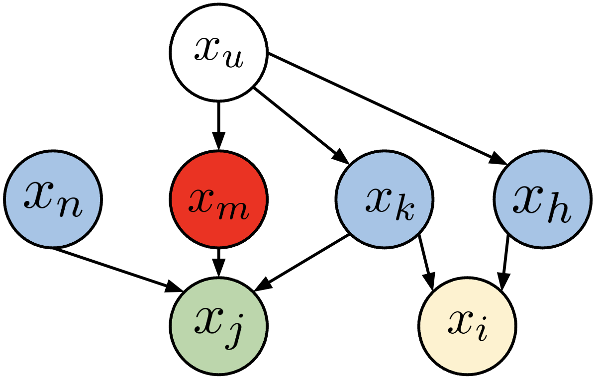
Figure 3: Exemplary DAG where $x_{u}$ is unobserved, $x_{m}$ is a proxy of $x_{k},x_{h}$, $x_{j}$ is MRD-I, and $x_{i}$ is MRD-N.

we iteratively check every triplet of dependent variables for whether one variable is a proxy for the other two, using the procedure provided by Liu et al., (2024). We then identify at least two independent root ancestors of each MRD-N in Lemma 4.2 (proof in Appendix D.9):

Lemma 4.2.

Under the existence of a root proxy, $x_{i}$ is an MRD-N iff it induces a VP with at least two of its root ancestors after all proxy variables are leveraged.

1:Input: vertices $x_{1},\ldots,x_{d}\in V$.

2:Initialize: root set $RT$, root superset $W$.

3:Stage 1: Prune MRDs, Obtain Some Roots

4:Run pairwise $\perp\!\!\!\perp$ tests between each pair of vertices $x_{i},x_{j}\in V$ and remove all MRD-I from $V$.

5:Check each dependant triplet of vertices for whether one is a proxy for the other two using procedure of Liu et al., (2024); remove all MRD-N to obtain $V^{\prime}$.

6:Add any vertex $x_{i}\in V^{\prime}$ to $RT$ if $x_{i}\perp\!\!\!\perp x_{j}\forall x_{j}\in V^{\prime}\setminus{\{x_{i}\}}$, and remove all $x_{i}$ from $V^{\prime}$ to obtain $V^{\prime\prime}$.

7:Stage 2: Prune SRDs, Obtain Roots

8:Run pairwise nonparametric regression between $x_{i},x_{j}\in V^{\prime\prime}$; if $\exists x_{l}$ such that $x_{k}\in V^{\prime\prime}$ is identified as $\in\text{An}(x_{j})$, and there does not exist $x_{h}$ such that $x_{h}$ is identified $\in\text{An}(x_{k})$, add $x_{k}$ to $W$.

9:For each $x_{i},x_{j}\in W$ such that $x_{i}\not\!\perp\!\!\!\perp x_{j}$, for all $x_{k}$ such that $x_{j}$ is identified $\in\text{An}(x_{k})$ regress $x_{k}$ onto $x_{i},x_{j}$ and collect the residual; add any $x_{i}$ that is always independent of the residual to $RT$.

10:Stage 3: Recover Sort

11:Run Sort Finder (Alg 2) using $RT$, obtain $\pi$.

12:return $\pi$

Algorithm 4 LoSAM-UV

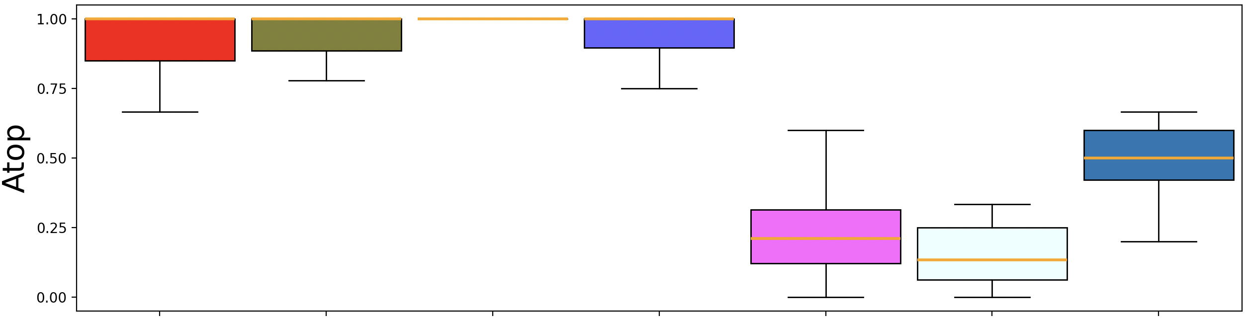
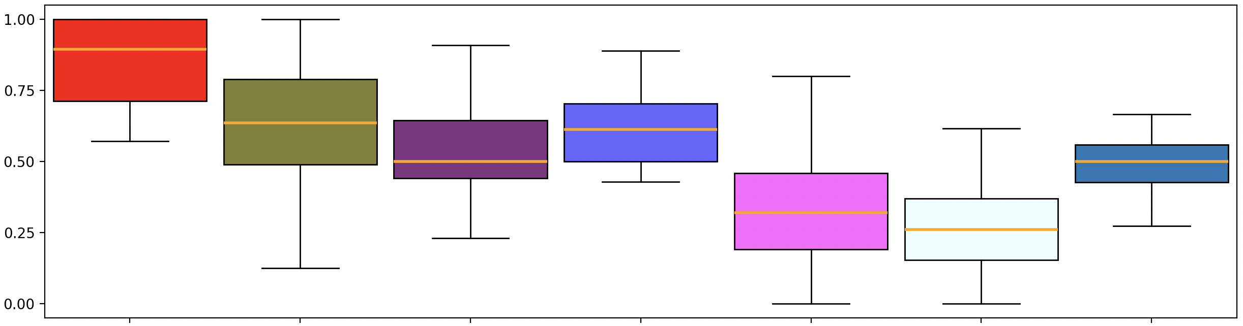
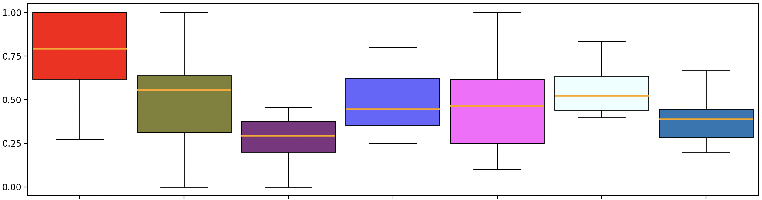
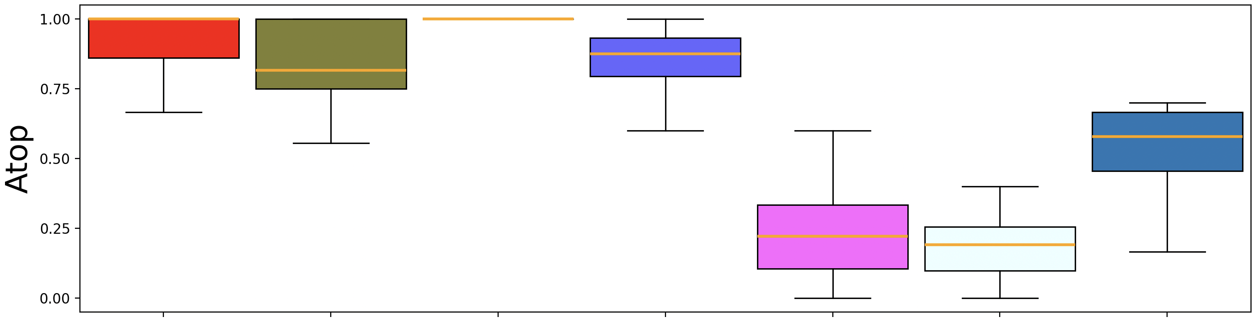
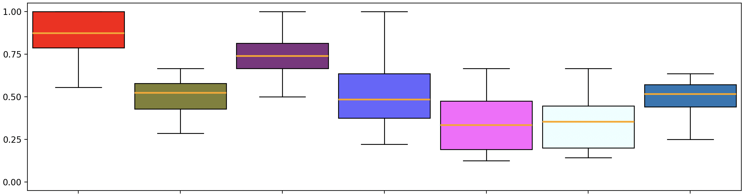
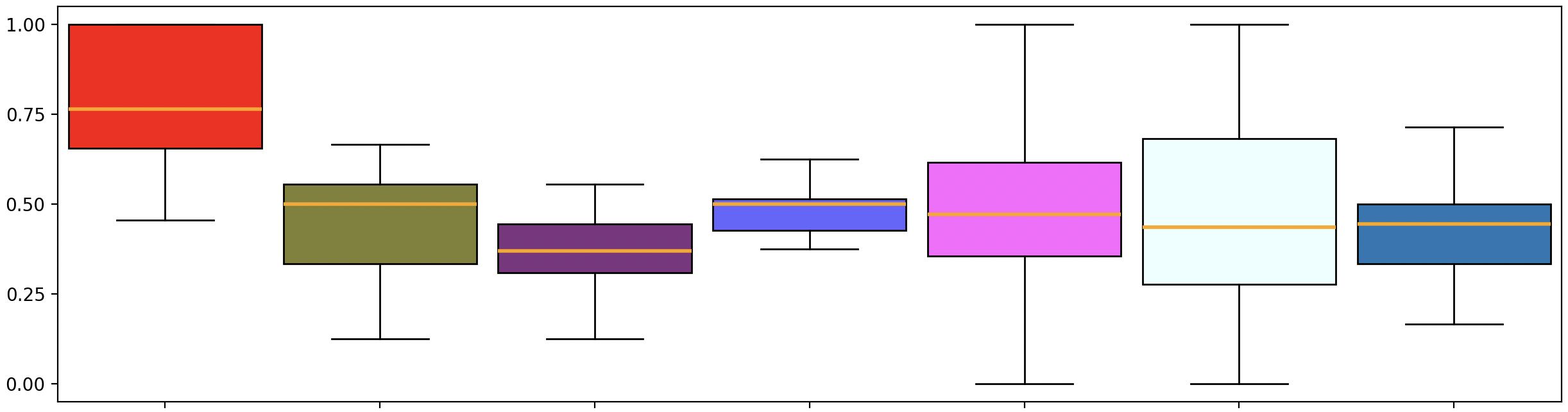
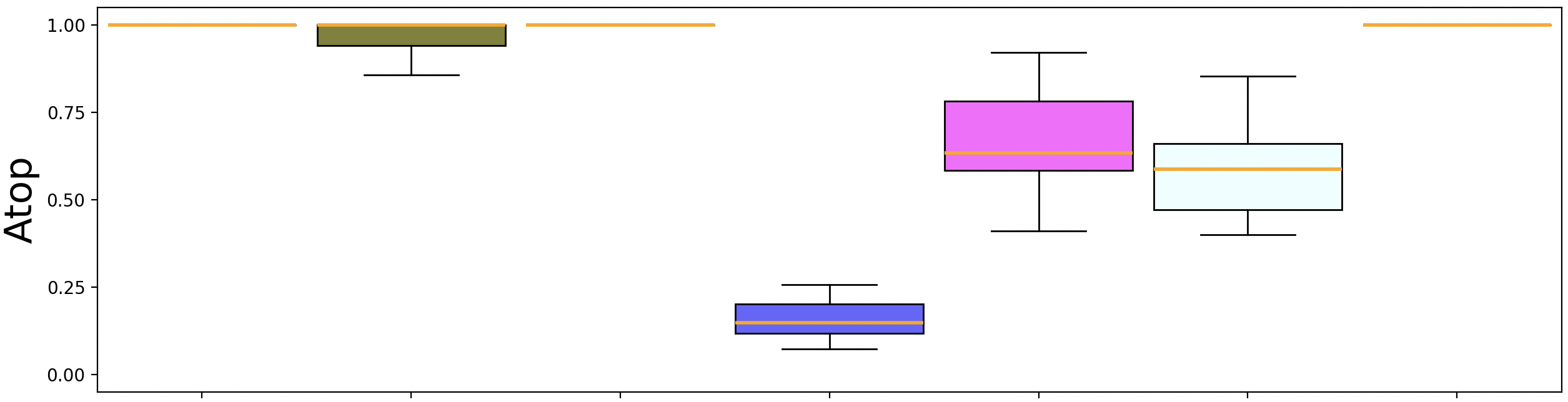
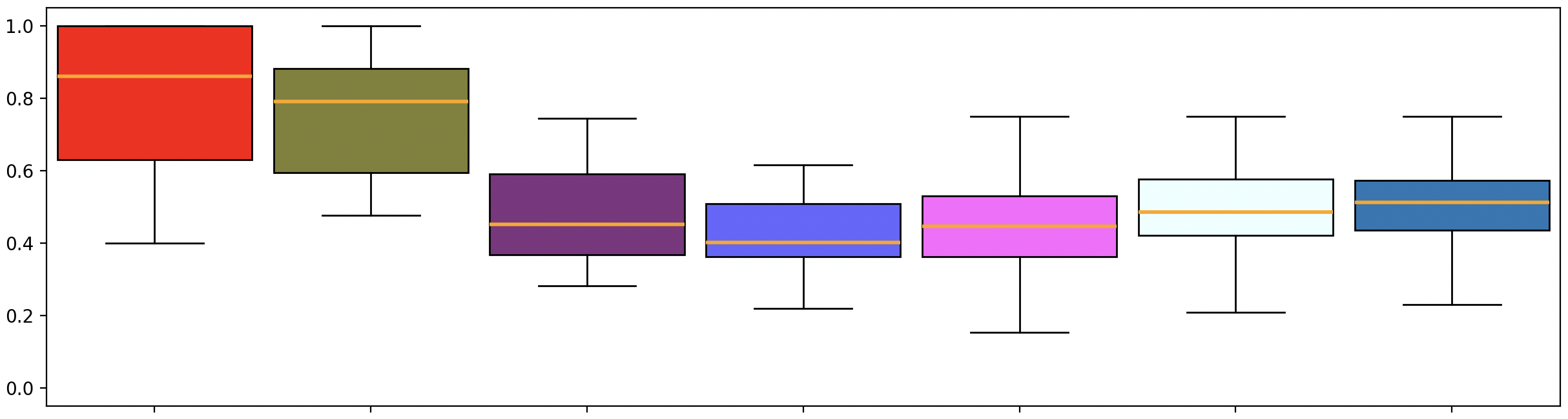
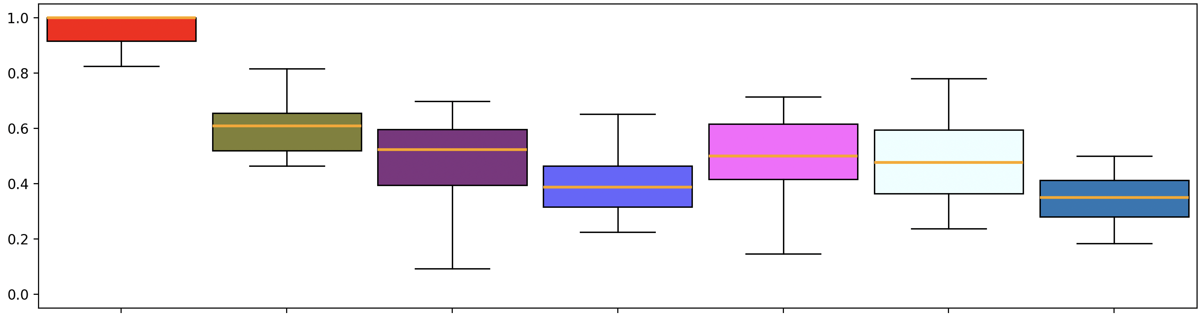
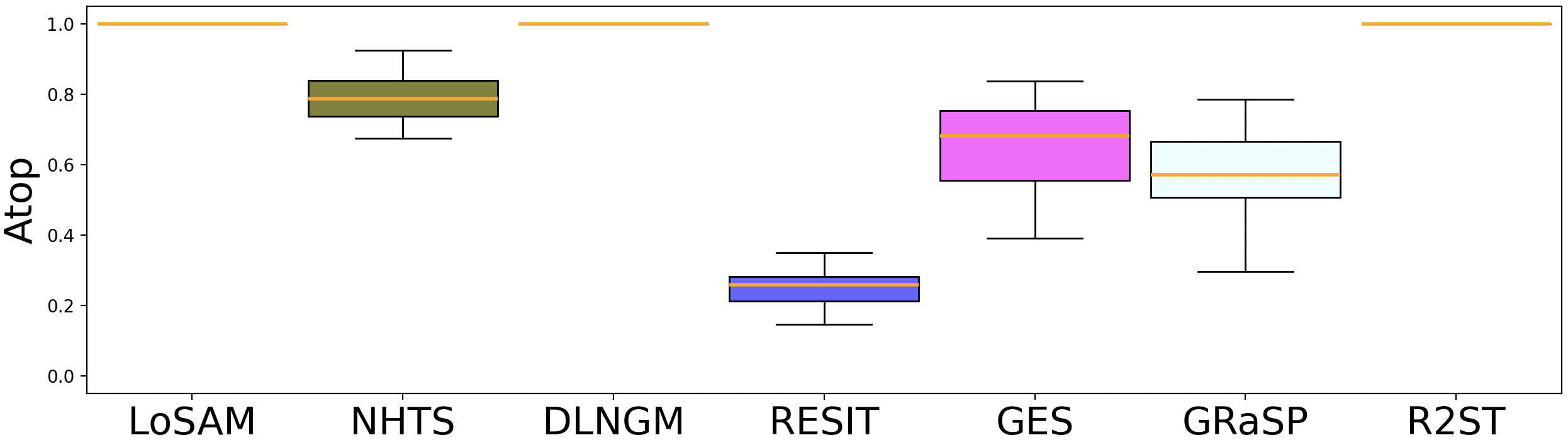
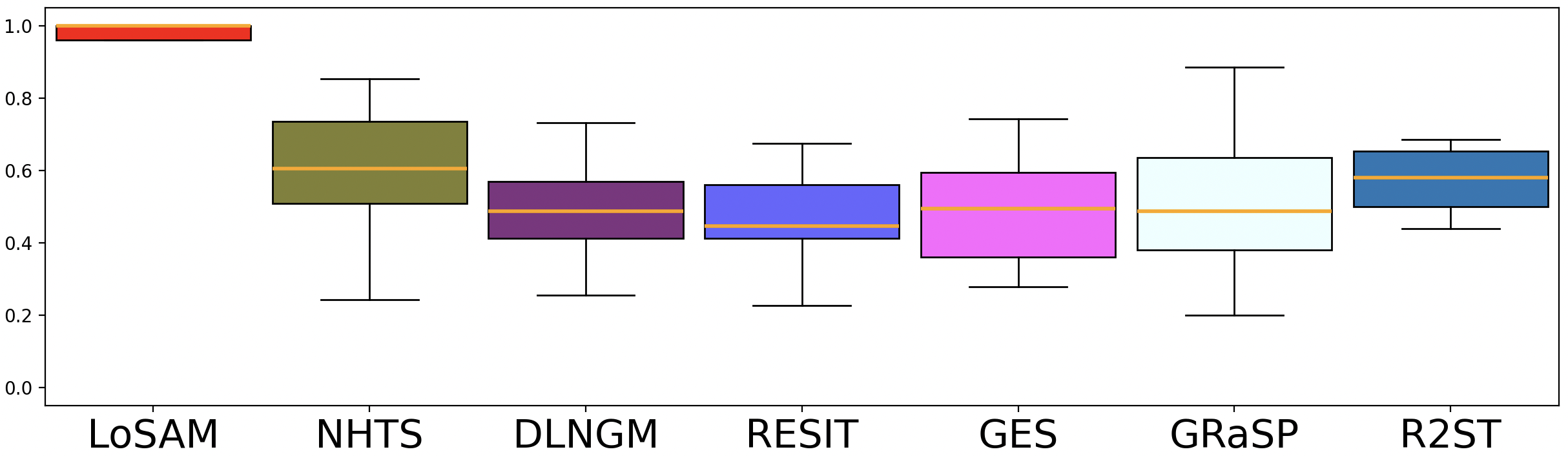
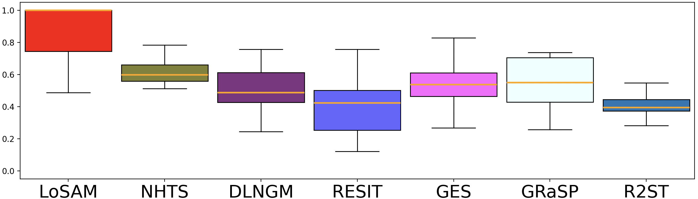
Figure 4: Performance of LoSAM on data generated with linear (left column), mixed (middle column), and nonlinear (right column) causal mechanisms, sparse (top two rows) and dense (bottom two rows) DAGs, and Uniform (rows one, three) or Laplace (rows two, four) error distributions. See Appendix G.3 for runtime results.

SRD Pruning 

Having pruned all MRDs (MRD-I and MRD-N), we are left with SRDs and roots in the set $V^{\prime}$. Similar to Alg 1, we identify all roots with no SRDs $\in V^{\prime}$ by using Lemma 3.2, obtaining the subset $V^{\prime\prime}\subseteq V^{\prime}$, and identify a superset of roots with SRDs $W\subseteq V^{\prime\prime}$ by using the Ancestor-Descendant test in Definition 3.4. It remains to prune SRDs from $W$.

We observe that when latent confounders between roots exist, Lemma 3.3 may fail. Recall that Lemma 3.3 relies on the fact that no root can d-separate any of its SRDs from every other vertex in $W$ that is dependent on the root. However, this no longer holds when the roots are confounded. In particular, if two roots are latently confounded, one root could d-separate any of its SRDs from the other root. Appendix I.3 formally states and illustrates this problem.

To address this, we prune the root superset $W$ using bivariate nonparametric regressions rather than conditional independence:

Lemma 4.3.

All roots are contained in $W$. For $x_{i},x_{j},x_{k}\in V$, let $r_{ij}^{k}$ be the residual of $x_{k}$ nonparametrically regressed onto both $x_{i}$ and $x_{j}$. Then, vertex $x_{i}\in W$ is a root vertex if and only if for every other vertex $x_{j}\in W$ such that $x_{i}\not\!\perp\!\!\!\perp x_{j}$, $\forall x_{k}$ such that $x_{j}$ is identified $\in\text{An}(x_{k})$, we have $x_{j}\perp\!\!\!\perp r_{ij}^{k}$.

Lemma 4.3 relies on the intuition if $x_{i}\in W$ is a root (a nondescendant of any vertex in $W$), then adding it as a covariate should not change the independence results of any pairwise regression. However, the reverse does not hold for any non-root SRD: the inclusion of these variables in the bivariate regression would yield at least one dependent residual when the regression involves its ancestor. We formally state this intuition mathematically in Appendix D.10.

Putting together changes to both MRD and SRD pruning, we present LoSAM-UC in Algorithm 4, a method that can handle latent confounders between roots.

We show the correctness of Algorithm 4 in Theorem 4.4 (proof in Appendix F.4), the worst-case time complexity in Theorem 4.5 (proof in Appendix F.5), and a detailed example in Appendix H.2.

Theorem 4.4.

Given a graph $G$, Algorithm 4 asymptotically finds a correct topological sort of $G$.

Theorem 4.5.

Given $n$ samples of $d$ vertices generated by an ANM, the worst case runtime complexity of Algorithm 4 is upper bounded by $O(d^{3}n^{3})$.

5 Experimental Results

Setup

We test our method across a wide selection of synthetic data settings, varying the graph sparsity, exogenous error distribution, and causal mechanisms. DAGs are randomly generated with the Erdos-Renyi model (Erdos and Renyi,, 1960); the average number of edges in each $d$-dimensional DAG is either $d$ (ER1) for sparse DAGs, or $4d$ (ER4) for dense DAGs. Uniform or Laplace noise is used as the exogenous error. We randomly sample the data ($d=10,n=300$) according to causal mechanisms that are either entirely linear, entirely nonlinear, or are mixed, with each vertex having linear or nonlinear mechanisms with probability $\frac{1}{2}$. Similar to recent related literature (Lippe et al.,, 2022; Ke et al.,, 2023), the nonlinear functions are parameterized by a neural network with random weights. We process the data to ensure that the simulated data is sufficiently challenging (Appendix G.1). Methods are evaluated on 20 DAGs in each experiment.

Metrics

$A_{top}$ is equal to the percentage of edges that can be recovered by the returned topological ordering (an edge cannot be recovered if a child is sorted before a parent) (Hiremath et al.,, 2024). We note that $A_{top}$ is a normalized version of the topological ordering divergence $D_{top}$ defined in Rolland et al., (2022). Note that the scoring-based approaches (GES, GRaSP) return a MEC, rather than a unique DAG; similar to prior work (Montagna et al., 2023a, ), we randomly select one topological ordering permitted by the returned MEC for evaluation, to enable fair comparison.

LoSAM Performance

Figure 4 demonstrates the performance of our topological ordering algorithm LoSAM; we take NHTS (Hiremath et al.,, 2024), DirectLiNGAM (Shimizu et al.,, 2011), RESIT (Peters et al.,, 2014), GES (Chickering,, 2002), and GRaSP (Lam et al.,, 2022) as baseline comparators that are agnostic to the noise distribution. We include the heuristic algorithm $R^{2}$-Sort (Reisach et al.,, 2023) as a measure of the gameability of the synthetic data (see Appendix G.1). We find that LoSAM outperforms all baselines (including the original local search method NHTS) in all experiments with nonlinear or mixed ANM, achieving the highest median $A_{top}$ in all trials. The enhanced performance in the nonlinear setting is likely attributed to increased stability with finite samples, achieved through the use of novel test statistics. Further, we test the robustness of LoSAM under linear data-generating mechanisms (Figure 4 left column). We observe that LoSAM outperformed all nonlinear baselines and achieved similar performance to DirectLiNGAM, a specialized method that leverages the linearity property. Additionally, we note that, as expected from Theorem 3.6, LoSAM had higher computational efficiency than NHTS, running $2-5\times$ faster across experiments (see Appendix G.3).

Discussion

In this paper, we developed two novel topological ordering algorithms for use in global causal discovery. LoSAM (Alg 3) improved on previous local search topological ordering methods by extending asymptotic guarantees from nonlinear ANMs to the full ANM setting while improving sample efficiency; we then adapted LoSAM to be resistant to latent confounding, developing LoSAM-UC (Alg 4). We tested LoSAM across a range of robustly generated synthetic data, finding that our method systematically outperformed baselines. Future work includes extending LoSAM-UC to handle latent confounding of non-roots, and applying the local search approach to a time series setting.

Checklist

1. For all models and algorithms presented, check if you include:

   1. A clear description of the mathematical setting, assumptions, algorithm, and/or model.
      Yes. Justification: see Section 2, Appendix C for mathematical setting and assumptions, and Sections 3, 4 for algorithm and model.

   2. An analysis of the properties and complexity (time, space, sample size) of any algorithm.
      Yes. Justification: see Sections 3.3, 4.

   3. (Optional) Anonymized source code, with specification of all dependencies, including external libraries.
      Yes. Justification: see supplementary material.

2. For any theoretical claim, check if you include:

   1. Statements of the full set of assumptions of all theoretical results.
      Yes. Justification: see Section 2, Appendix C.

   2. Complete proofs of all theoretical results.
      Yes. Justification: see Appendix D, E, and F.

   3. Clear explanations of any assumptions.
      Yes. Justification: see Appendix C.

3. For all figures and tables that present empirical results, check if you include:

   1. The code, data, and instructions needed to reproduce the main experimental results (either in the supplemental material or as a URL).
      Yes. Justification: see supplementary material.

   2. All the training details (e.g., data splits, hyperparameters, how they were chosen).
      Yes. Justification: see Appendix G.2.

   3. A clear definition of the specific measure or statistics and error bars (e.g., with respect to the random seed after running experiments multiple times).
      Yes. Justification: see Appendix G.2.

   4. A description of the computing infrastructure used. (e.g., type of GPUs, internal cluster, or cloud provider).
      Yes. Justification: see Appendix G.2.

4. If you are using existing assets (e.g., code, data, models) or curating/releasing new assets, check if you include:

   1. Citations of the creator If your work uses existing assets.
      Yes. Justification: see Appendix K.

   2. The license information of the assets, if applicable.
      Yes. Justification: see Appendix K.

   3. New assets either in the supplemental material or as a URL, if applicable.
      Yes. Justification: see supplemental material.

   4. Information about consent from data providers/curators.
      Not Applicable.

   5. Discussion of sensible content if applicable, e.g., personally identifiable information or offensive content.
      Not Applicable.

5. If you used crowdsourcing or conducted research with human subjects, check if you include:

   1. The full text of instructions given to participants and screenshots.
      Not Applicable.

   2. Descriptions of potential participant risks, with links to Institutional Review Board (IRB) approvals if applicable.
      Not Applicable.

   3. The estimated hourly wage paid to participants and the total amount spent on participant compensation.
      Not Applicable.

 

APPENDIX

 

Appendix A NOTATION

$G=(V,E)$

A DAG $G$ with $|V|=d$ vertices, where $E$ represents the set of directed edges between vertices.

$\mathrm{Ch}(x_{i})$

The set of child vertices of $x_{i}$.

$\mathrm{Pa}(x_{i})$

The set of parent vertices of $x_{i}$.

$\mathrm{De}(x_{i})$

The set of vertices that are descendants of $x_{i}$.

$\mathrm{An}(x_{i})$

The set of vertices that are ancestors of $x_{i}$.

$\pi$

A topological ordering of vertices, i.e. a mapping $\pi:V\rightarrow\{0,1,\ldots,d\}$.

$f_{i}$

An arbitrary function, used to generate vertex $x_{i}$.

$\varepsilon_{i}$

An independent noise term sampled from an arbitrary distribution, used to generate vertex $x_{i}$.

$\mathrm{SRD}$

A single root descendant, a vertex with only one root ancestor.

$\mathrm{MRD}$

A multi root descendant, a vertex with at least two root ancestors.

$\mathrm{VP}$

A v-pattern, a causal substructure between three vertices.

$V^{\prime}$

A subset of $V$ that contains only and all roots and SRDs.

$V^{\prime\prime}$

A subset of $V^{\prime}$ that contains only and all SRDs and roots with at least one SRD.

$r_{ij}$

The residual of the vertex $x_{j}$ nonparametrically regressed on the vertex $x_{i}$.

$W$

A subset of $V^{\prime\prime}$ that contains only and all vertices identified by the Ancestor-Descendant Test.

$M$

The set of MRDs in $V$.

$R$

The set of roots in $V$.

$c^{\mathrm{Alg1}}_{\mathrm{max}}$

The maximum size of conditioning sets used in Algorithm 1.

$c^{\mathrm{NHTS}}_{\mathrm{max}}$

The maximum size of conditioning sets used in the root identification step of NHTS.

$U$

The set of vertices left unsorted, i.e., not yet added to $\pi$.

$\mathrm{VC}$

A valid candidate; a vertex in $U$ with no parents in $U$.

$U_{E}$

The set of residuals produced from regressing each $x_{i}\in U$ onto vertices in $\pi$.

$e_{i}$

A residual in $U_{E}$ corresponding to $x_{i}\in U$.

$\mathrm{ND}$

A nonlinear descendant; a vertex in $U$ that is a nonlinear function of at least one vertex in $U$.

$\mathrm{LD}$

A linear descendant; a vertex in $U$ that is a linear function of all vertices in $U$.

$q_{ij}$

The residual produced by linearly regressing $e_{j}$ onto $e_{i}$.

$Q$

A subset of $U$ that contains all LDs, but no VCs.

$U^{\prime}$

A subset of $U$ that contains all VCs and some NDs.

$\widehat{MI}(x,y)$

A nonparametric estimator of mutual information between $x,y$.

$t^{*}(e_{i},\pi)$

A test statistic corresponding to $x_{i}\in U^{\prime}$.

$\mathrm{MRD-I}$

A multi root descendant that has at least two unconfounded root ancestors.

$\mathrm{MRD-N}$

A multi root descendant whose root ancestors are all mutually confounded.

$r_{ij}^{k}$

The residual produced by nonparametrically regressing $x_{k}$ onto $x_{i},x_{j}$.

Appendix B GRAPH TERMINOLOGY

In this section we clarify the term ‘d-separation’, a foundational concept for analyzing causal graphical models (Spirtes et al.,, 2000). First, we classify the types of paths that exist between vertices, then define d-separation in terms of those paths.

We first note that a path between $x_{i},x_{k}$ can either start and end with an edge out of $x_{j},x_{k}$ ($x_{k}\dashrightarrow\cdots\dashleftarrow x_{k}$), start with an edge of out of $x_{j}$ and end with an edge into $x_{k}$ ($x_{j}\dashrightarrow\cdots\dashrightarrow x_{k}$) or start with an edge into $x_{j}$ and edge with an edge into $x_{k}$ ($x_{j}\dashleftarrow\cdots\dashrightarrow x_{k}$). Paths such as $x_{k}$ ($x_{k}\dashrightarrow\cdots\dashleftarrow x_{k}$) do not transmit causal information between $x_{j},x_{k}$. Undirected paths that transmit causal information between two vertices $x_{j},x_{k}$ can be differentiated into frontdoor and backdoor paths (Spirtes et al.,, 2000). A frontdoor path is a directed path $x_{j}\dashrightarrow\cdots\dashrightarrow x_{k}$, while a backdoor path is a path $x_{j}\dashleftarrow\cdots\dashrightarrow x_{k}$.

Paths between two vertices are further classified, relative to a vertex set Z, as either active or inactive (Spirtes et al.,, 2000). A path between vertices $x_{j},x_{k}$ is active relative to Z if every node on the path is active relative to Z. Vertex $x_{i}\in V$ is active on path relative to Z if one of the following holds: 1) $x_{i}\in\textbf{Z}$ and $x_{i}$ is a collider 2) $x_{i}\not\in\textbf{Z}$ and $x_{i}$ is not a collider 3) $x_{i}\not\in\textbf{Z}$, $x_{i}$ is a collider, but $\text{De}(x_{i})\cap\textbf{Z}\neq\emptyset$. An inactive path is simply a path that is not active. Causally paths are typically described active or inactive with respect to $\textbf{Z}=\emptyset$ unless otherwise specified.

Vertices $x_{i},x_{j}$ are said to be d-separated by a set Z iff there is no active path between $x_{i},x_{j}$ relative to $Z$.

Appendix C ASSUMPTIONS

C.1 Causal Markov

The Causal Markov condition implies that a variable $x_{i}$ is independent of all non-descendants $x_{j}$, given its parents $\text{Pa}(x_{i})$ (Spirtes,, 2001). Equivalently, we say that an ANM $G=(V,E)$ satisfies the Causal Markov Condition if the joint distribution $p_{V}(V)$ over all $x_{i}\in V$ admits the following factorization:

$$p_{V}(V)=\prod_{i}^{d}p_{i}(x_{i}|\text{Pa}(x_{i})).$$ (3)

C.2 Acyclicity

We say that a causal graph $G$ is acyclic if there does not exist any directed cycles in $G$ (Spirtes,, 2001).

C.3 Faithfulness

Note that by assuming that a causal graph $G$ satisfies the Causal Markov assumption, we assume that data produced by the DGP of $G$ satisfies all independence relations implied by $G$ (Spirtes,, 2001). However, this does not necessarily imply that all independence relations observed in the data are implied by $G$. Under the assumption of faithfulness, the independence relations implied by $G$ are the only independence relations found in the data generated by $G$’s DGP (Spirtes,, 2001).

C.4 Identifiability of ANM

Following the style of (Montagna et al., 2023a, ), we first observe that the following condition guarantees that the observed distribution of a pair of variables $x_{i},x_{j}$ can only be generated by a unique ANM:

Condition C.1 (Hoyer and Hyttinen, (2009)).

Given a bivariate model $x_{i}=\varepsilon_{i},x_{j}=f_{j}(x_{i})+\varepsilon_{j}$ generated according to (1), we call the SEM an identifiable bivariate ANM if the triple $(f_{i},p_{\varepsilon_{i}},p_{\varepsilon_{j}})$ does not solve the differential equation $k^{\prime\prime\prime}=k^{\prime\prime}(-\frac{g^{\prime\prime\prime}f^{\prime}}{g^{\prime\prime}}+\frac{f^{\prime\prime}}{f^{\prime}})-2g^{\prime\prime}f^{\prime\prime}f^{\prime}+g^{\prime}f^{\prime\prime\prime}+\frac{g^{\prime}g^{\prime\prime\prime}f^{\prime\prime}f^{\prime}}{g^{\prime\prime}}-\frac{g^{\prime}(f^{\prime\prime})^{2}}{f^{\prime}}$ for all $x_{i},x_{j}$ such that $f^{\prime}(x_{i})g^{\prime\prime}(x_{j}-f_{j}(x_{i}))\neq 0$, where $p_{\varepsilon_{i}},p_{\varepsilon_{j}}$ are the density of $\varepsilon_{i},\varepsilon_{j}$, $f=f_{j},k=\log p_{\varepsilon_{i}},g=p_{\varepsilon_{j}}$. The arguments $x_{j}-f_{j}(x_{i}),x_{i}$ and $x_{i}$ of $g,k$ and $f$ respectively, are removed for readability.

There is a generalization of this condition to the multivariate ANM proved by (Peters et al.,, 2014):

Theorem C.2.

(Peters et al. (Peters et al.,, 2014)). An ANM corresponding to DAG $G$ is identifiable if $\forall x_{j}\in V,x_{i}\in\text{Pa}(x_{j})$ and all sets $S\subseteq V$ with $\text{Pa}(x_{j})\setminus\{i\}\subseteq S\subseteq\overline{\text{De}(j)}\setminus{\{x_{i},x_{j}\}}$, $\exists$ $X_{S}$ with positive joint density such that the triple $\Big{(}f_{j}(\text{Pa}(j)\setminus{\{x_{i}\}},x_{i}),p_{x_{i}|X_{s}},p_{\varepsilon_{j}}\Big{)}$ satisfies Condition C.1, and $f_{j}$ are non-constant in all arguments.

In this paper, we assume that all DAGs are generated by identifiable ANMs, as defined in Theorem C.2.

Appendix D LEMMA PROOFS

D.1 Proof of Lemma 3.1

See 3.1

Proof.

Suppose $x_{i}$ is an MRD. Then, $\exists x_{j},x_{k}$ such that $x_{j},x_{k}\in\text{An}(x_{i})$, and $x_{j},x_{k}$ are roots. Note that this implies that $x_{j}\perp\!\!\!\perp x_{k},x_{i}\not\!\perp\!\!\!\perp x_{j},x_{i}\not\!\perp\!\!\!\perp x_{k}$, which is a VP between $x_{j},x_{k}$ induced by $x_{i}$.

Suppose $x_{i}$ is not an MRD. We prove by contradiction that $x_{i}$ cannot induces a VP.

Suppose $x_{i}$ is an SRD. Let $x_{p}$ be any vertex such that $x_{p}\not\!\perp\!\!\!\perp x_{i}$, which implies that there must exist an active causal path between $x_{i},x_{p}$. Note, as $x_{i}$ is an SRD, there exists only one root vertex $x_{j}$ such that $x_{j}\in\text{An}(x_{i})$. Suppose for contradiction that $x_{p}\not\in\text{De}(x_{j})$. Suppose there is a frontdoor path from $x_{i}$ to $x_{p}$: then $x_{p}\in\text{De}(x_{i})\implies x_{p}\in\text{De}(x_{j})$, which contradicts our assumption that $x_{p}\not\in\text{De}(x_{j})$. Suppose there is a frontdoor path from $x_{p}$ to $x_{i}$: as $x_{p}\not\in\text{De}(x_{j})$, WLOG $\exists$ a root $x_{m}\neq x_{j}$ such that $x_{p}\in\text{De}(x_{m})$. This implies that $x_{i}\in\text{De}(x_{m})$ which contradicts the assumption that $x_{i}$ is an SRD. Suppose for contradiction that there exists a backdoor path between $x_{p},x_{i}$: this implies that $\exists$ $x_{c}$ that is a confounder between $x_{p},x_{i}$. Again, this implies that WLOG $\exists$ a root $x_{m}\neq x_{j}$ such that $x_{c}\in\text{De}(x_{m})\implies x_{i}\in\text{De}(x_{m})$, which contradicts the assumption that $x_{i}$ is an SRD. Therefore, it must be that, for any vertex $x_{p}\not\!\perp\!\!\!\perp x_{i}$, $x_{i},x_{p}\in\text{De}(x_{j})$, where $x_{j}$ is a root. Note, the above implies that for any vertices $x_{j},x_{k}$ such that $x_{j}\not\!\perp\!\!\!\perp x_{i},x_{k}\not\!\perp\!\!\!\perp x_{i}$, we have $x_{j},x_{k}\in\text{De}(x_{j})\implies x_{j}\not\!\perp\!\!\!\perp x_{k}$. This implies that $x_{i}$ cannot induce a VP between any two vertices $x_{j},x_{k}$.

Suppose $x_{i}$ is a root. Let $x_{j},x_{k}$ be any two vertices such that $x_{j}\not\!\perp\!\!\!\perp x_{i},x_{k}\not\!\perp\!\!\!\perp x_{i}$. Note that as $x_{i}$ is a root, there can only exist frontdoor paths between $x_{i}$ and other vertices, so the dependence relations imply that $x_{j},x_{k}\in\text{De}(x_{i})$. This means that $x_{i}$ is a confounder of $x_{j},x_{k}\implies x_{j}\not\!\perp\!\!\!\perp x_{k}$. Therefore, $x_{i}$ cannot induce a VP between $x_{j},x_{k}$. ∎

D.2 Proof of Lemma 3.2

See 3.2

Proof.

Note that $V^{\prime}$ is the union of vertices that are either SRDs or root vertices. We prove this by contradiction. Suppose that $x_{i}$ is an SRD: then $\exists x_{k}\in V^{\prime}$ such that $x_{k}$ is a root and $x_{i}\in\text{De}(x_{k})$ which implies $x_{i}\not\!\perp\!\!\!\perp x_{k}$. However, this contradicts our assumption that $x_{i}\perp\!\!\!\perp x_{j},\forall x_{j}\in V^{\prime}$. Now we show that $x_{i}$ cannot a root vertex with SRDs. Suppose that $x_{i}$ is a root vertex with SRDs: then $\exists x_{k}\in\text{De}(x_{i})\implies x_{i}\not\!\perp\!\!\!\perp x_{k}$. However, this contradicts our assumption that $x_{i}\perp\!\!\!\perp x_{j},\forall x_{j}\in V^{\prime}$. Additionally, note that a root vertex $x_{i}$ with no SRDs satisfies $x_{i}\perp\!\!\!\perp x_{j},\forall x_{j}\in V^{\prime}$. Therefore, $x_{i}$ must be a root vertex with no SRDs. ∎

D.3 Proof of Lemma 3.3

See 3.3

Proof.

In this proof, we say that $x_{i}$ is in ‘AD relation’ to $x_{k}$ iff $x_{i}$ is identified as $\in\text{An}(x_{k})$ by the Ancestor Descendant test (Definition 3.4).

By definition, any root vertex $x_{i}\in V^{\prime\prime}$ has at least one SRD $x_{j}\in V$, such that $x_{j}\in\text{Ch}(x_{i})$. Note that as $x_{j}=f_{ij}(x_{i})+\varepsilon_{j}$, $x_{i}$ is in AD relation to $x_{j}$. Note that as $x_{i}$ is a root vertex, all $x_{j}\in V^{\prime\prime}$ are either independent of $x_{i}$ or descendants of $x_{i}$. If $x_{j}\perp\!\!\!\perp x_{i}$, then $x_{j}$ will not be in AD relation to $x_{i}$ as $x_{i}\perp\!\!\!\perp r_{i}^{j}$, violating condition 2) in the AD definition. If $x_{j}\not\!\perp\!\!\!\perp x_{i}$, then $x_{j}\in\text{De}(x_{i})$, and therefore by assumption of ANM C.2 we have that $x_{j}\not\!\perp\!\!\!\perp r_{j}^{i}$, implying that $x_{j}$ is not in AD relation to $x_{i}$. This implies that all root vertices in $V^{\prime\prime}$ satisfy condition 1) and 2) of the definition of $W$, implying that all root vertices in $V^{\prime\prime}$ are contained in $W$.

Suppose $x_{i}\in W$ is a root vertex. Let $x_{j}\in W$ such that $x_{i}\not\!\perp\!\!\!\perp x_{j}$. Note that as $x_{j}\in W,x_{j}\not\!\perp\!\!\!\perp x_{i}$, $x_{j}$ must be an SRD of $x_{i}$, and $x_{i}$ is not in AD relation to $x_{j}$. This implies that $x_{j}\in\text{De}(x_{i})$ but $x_{j}\not\in\text{Ch}(x_{i})$. In particular, note that $\forall x_{k}$ such that $x_{k}\in\text{Ch}(x_{i})$, $x_{i}$ is AD relation to $x_{k}$. Therefore, there must exist at least one $x_{k}$ such that $x_{j}\in\text{De}(x_{k})$, which implies that $x_{k}\not\!\perp\!\!\!\perp x_{j}|x_{i}$, implying that $x_{i}$ satisfies the second set of conditions 1) and 2).

Suppose $x_{i}\in W$ is not a root. Suppose for contradiction that the second set of conditions 1) and 2) are satisfied by $x_{i}$. Let $x_{k}$ be any vertex such that $x_{i}$ is in AD relation to $x_{k}$. Note that $\exists x_{j}\in W$ such that $x_{j}$ is a root, and $x_{j}\not\!\perp\!\!\!\perp x_{i}$. Note that, all active paths between $x_{i}$ and $x_{k}$ must be frontdoor paths, and $x_{j}$ must lie along all paths: if not, then $x_{i}$ would be a confounder of $x_{j},x_{k}$, and therefore $x_{j}$ would not be in AD relation to $x_{k}$. This implies that $x_{i}\perp\!\!\!\perp x_{k}|x_{j}$, which contradicts condition 2).Therefore, the second set of conditions 1) and 2) cannot be simultaneously satisfied by nonroots. ∎

D.4 Proof of Lemma 3.4

See 3.4

Proof.

Suppose $x_{i}\in U$ is a ND. Then, by definition $\exists x_{j}\in U$ such that $x_{j}$ is a nonlinear function of its parents in $U$ ($\text{Pa}(x_{j})\cap U$), and $x_{j}$ is an ancestor of $ND$ ($x_{j}\in\text{An}(x_{i}$). Note that this implies that the regression of $x_{i}$ onto sorted vertices $\pi$ leads to omitted variable bias (Pearl et al.,, 2016), which leads to $e_{i}$ being dependent on any sorted vertex $x_{k}\in\pi$ such that $x_{k}$ is an ancestor of $x_{j}$ ($x_{k}\in\text{An}(x_{j})$). Therefore, $e_{i}$ is dependent on at least one sorted vertex in $\pi$.

Suppose $e_{i}$ is dependent on at least on sorted vertex in $\pi$. Note that by assumption there are only nonlinear functions, $x_{i}$ is not an LD. Suppose for contradiction that $x_{i}$ is a VC. Then, $x_{i}=f_{i}(\text{Pa}(x_{i}))+\varepsilon_{i}$. Note that as $\pi$ is a valid topological sort, it follows that $\text{Pa}(x_{i})\subseteq\pi$ and $\text{De}(x_{i})\cap\pi=\emptyset$. Therefore, $e_{i}=\varepsilon_{i}$, which implies $e_{i}\perp\!\!\!\perp x_{j},\forall x_{j}\in\pi$. This implies that $e_{i}$ is independent of all vertices in $\pi$, contradicting our above assumption.

∎

D.5 Proof of Lemma 3.5

See 3.5

Proof.

Let $x_{i}\in U$ be a LD. This implies that we can decompose $x_{i}$ into a potentially nonlinear function of its parents in $\pi$ and its the error terms of its ancestors in $U$:

$$x_{i}=f_{i}(\text{Pa}(x_{i})\cap\pi)+\sum_{x_{j}\in\text{An}(x_{i})\cap U}\alpha_{ij}\varepsilon_{j}+\varepsilon_{i}.$$ (4)

This implies that the residual of $x_{i}$ nonparametrically regressed onto $\pi$ equals

$$e_{i}=\sum_{x_{j}\in\text{An}(x_{i})\cap U}\alpha_{ij}\varepsilon_{j}+\varepsilon_{i}.$$ (5)

As $\varepsilon$ are mutually marginally independent, we have that $r_{i}\perp\!\!\!\perp x_{j},\forall x_{j}\in\pi$.

∎

D.6 Proof of Lemma 3.6

See 3.6

Proof.

Suppose $x_{i}\in U$ is an LD. Let $x_{j}\in U$ be an ancestor of $x_{i}$ such that $x_{j}$ has no parents in $U$, i.e. $\text{Pa}(x_{j})\cap U=\emptyset$. Such a vertex must always exist, as other $x_{i}$ would be a VC. We can decompose $x_{j}$ into a function of parents in $\pi$, and an independent error term:

$$x_{j}=f_{j}(\text{Pa}(x_{j})\cap\pi)+\varepsilon_{j}.$$ (6)

We can decompose $x_{i}$ into a function of parents in $\pi$, a sum of linear functions of parents in $U$, and the independent error term $\varepsilon_{i}$:

$$x_{i}=f_{i}(\text{Pa}(x_{i})\cap\pi)+\sum_{x_{j}\in\text{Pa}(x_{i})\cap U}\alpha_{ij}x_{j}+\varepsilon_{i}.$$ (7)

Note that as $x_{i}$ is a LD, all of its ancestors in $U$ are linear functions of their parents in $U$. Therefore, we can further decompose the sum of ancestors in $U$ as a linear sum of error terms:

$$x_{i}=f_{i}(\text{An}(x_{i})\cap S)+\sum_{x_{j}\in\text{An}(x_{i})\cap U}\beta_{ij}\varepsilon_{j}+\varepsilon_{i}.$$ (8)

Now, we consider the residuals $e_{i},e_{j}\in U_{E}$, which we can write as:

$$e_{j}=\varepsilon_{j}$$ (9)

and

$$e_{i}=\sum_{x_{j}\in\text{An}(x_{i})\cap U}\beta_{ij}\varepsilon_{j}+\varepsilon_{i}.$$ (10)

As $e_{i}$ is a linear function of $r_{e}$, we have that $e_{j}\perp\!\!\!\perp q_{ji},e_{i}\not\!\perp\!\!\!\perp q_{ij}$, implying that $x_{i}\in Q$. Therefore, $Q$ contains all LDs.

Let $x_{i}\in U$ be a VC. Then, we can write $x_{i}$ as the sum of a function of parents (which are all contained in $\pi$) and independent error term:

$$x_{i}=f_{i}(\text{Pa}(x_{i}))+\varepsilon_{i}.$$ (11)

Note that $e_{i}\in U_{E}$ is then just the independent error term:

$$e_{i}=\varepsilon_{i}.$$ (12)

Note that $e_{i}$ has no parents in $U_{E}$: therefore, for any vertex $x_{j}$ with associated residual $e_{j}\in U_{E}$, either $e_{i}\perp\!\!\!\perp e_{j}\implies e_{j}\perp\!\!\!\perp q_{ji},e_{i}\perp\!\!\!\perp q_{ij}$, or $e_{i}\not\!\perp\!\!\!\perp e_{j}\implies e_{j}\not\!\perp\!\!\!\perp q_{ji},e_{i}\not\!\perp\!\!\!\perp q_{ij}$. The last statement follows from the fact that if $e_{i}\not\!\perp\!\!\!\perp e_{j}$, as $e_{i}$ is an independent error term, $e_{j}$ must be a function of $e_{i}$; then, the conclusion follows by assumption of ANM C.2. Therefore, $x_{i}\not\in Q$, and therefore no VCs are included in $Q$. ∎

D.7 Proof of Lemma 3.7

See 3.7

Proof.

Note, $U^{\prime}$ contains only ND and VC vertices.

Suppose test stastistic $t^{*}(e_{i},S)$ asymptotically aproaches $0$ as $n\rightarrow\infty$. Suppose for contradiction that $e_{i}$ is not independent of $x_{j}\in\pi$. Note that this implies that the mutual information $\hat{MI}(x_{j},e_{i})\neq 0$, which contradicts our assumption that $t^{*}(e_{i},S)\rightarrow 0$.

Suppose $e_{i}$ is independent of all vertices in $S$. This implies that, for each $x_{j}\in\pi$ the mutual information approaches $0$: $\hat{MI}(x_{j},e_{i})\rightarrow 0$. This implies that the sum also approaches $0$: $t^{*}(e_{i},S)=\sum_{x_{j}\in\pi}\hat{MI}(x_{j},e_{i})\rightarrow 0$.

∎

D.8 Proof of Lemma 4.1

See 4.1

Proof of Lemma 4.1.

If $x_{i}\in V$ is an MRD-I, then $\exists x_{j},x_{k}$ that are both roots, and ancestors of $x_{i}$. This implies that $x_{i}\not\!\perp\!\!\!\perp x_{j},x_{i}\not\!\perp\!\!\!\perp x_{k},x_{j}\perp\!\!\!\perp x_{k}$, means that $x_{i}$ induces a V-pattern between $x_{j},x_{k}$.

Suppose $x_{i}\in V$ is not an MRD-I, i.e., is either an MRD-N, root or SRD. If $x_{i}$ is a root or SRD, it follows from Lemma 3.1 that $x_{i}$ does not induce a VP. Suppose $x_{i}$ is a MRD-N, i.e. all root ancestors of $x_{i}$ are confounded. First, note that for $x_{j},x_{k}$ to be dependent on $x_{i}$, they must either be a root ancestor of $x_{i}$ or be descendants of at least one of the root ancestors of $x_{i}$. Then, as all root ancestors of $x_{i}$ are mutually confounded by a latent variable, there must exist a backdoor path between $x_{j},x_{j}$. Therefore, $x_{j}\not\!\perp\!\!\!\perp x_{k}$, and thus an MRD-N $x_{i}$ cannot induce a VP.

∎

D.9 Proof of Lemma 4.2

See 4.2

Proof.

By assumption, we note that for at least two latently confounded root ancestors $x_{j},x_{k}$ of any MRD-N $x_{i}$, there exists $x_{p}$ that is a proxy variable of $x_{j},x_{k}$. Note that $x_{j},x_{k},x_{p}$ are all confounded by a latent confounder, and therefore they are all marginally dependent. Then, by employing the hypothesis testing procedure in (Liu et al.,, 2024), we recover that $x_{j}\perp\!\!\!\perp x_{k}$. As $x_{i}\not\!\perp\!\!\!\perp x_{j},x_{i}\not\!\perp\!\!\!\perp x_{k}$, this implies that $x_{i}$ induces a VP between $x_{j},x_{k}$.

Note, by assumption MRD-I have been pruned. Note, without latent confounding Lemma 3.1 shows that roots and SRDs do not induce VPs when there is no latent confounding. Note that after proxies are leveraged, the only independence results that are updated are those between some roots with proxies. This implies that the independence results still imply that roots and SRDs do not induce VPs. ∎

D.10 Proof of Lemma 4.3

See 4.3

Proof.

In this proof, we say that $x_{i}$ is in ‘AD relation’ to $x_{k}$ iff $x_{i}$ is identified as $\in\text{An}(x_{k})$ by the Ancestor Descendant test (Definition 3.4).

By definition, any root vertex $x_{i}\in V^{\prime\prime}$ has at least one SRD $x_{j}$, such that $x_{j}\in\text{Ch}(x_{i})$. Note that as $x_{j}=f_{ij}(x_{i})+\varepsilon_{j}$, $x_{i}$ is in AD relation to $x_{j}$. Note that as $x_{i}$ is a root vertex, all $x_{j}\in V^{\prime\prime}$ are not ancestors of $x_{i}$. If $x_{j}\perp\!\!\!\perp x_{i}$, then $x_{j}$ will not be in AD relation to $x_{i}$ as $x_{i}\perp\!\!\!\perp r_{ij}$, violating condition 2) in the AD definition. If $x_{j}\not\!\perp\!\!\!\perp x_{i}$, then $x_{j}\not\in\text{An}(x_{i})$, and therefore by assumption of the restricted ANM C.2 we have that $x_{j}\not\!\perp\!\!\!\perp r_{ji}$, implying that $x_{j}$ is not in AD relation to $x_{i}$. This implies that all root vertices in $V^{\prime\prime}$ satisfy condition 1) and 2) of the root superset $W$, implying that all root vertices in $V^{\prime\prime}$ are contained in $W$.

Let $x_{i}\in W$ be a root. Consider $x_{j}$ such that $x_{j}\not\!\perp\!\!\!\perp x_{i}$. Consider any $x_{k}$ such that $x_{j}$ is in AD relation to $x_{k}$. Note that $x_{j}\not\!\perp\!\!\!\perp x_{i}$ and $x_{i}$ being a root implies that $x_{i}$ is not a descendant of either $x_{j}$ or $x_{k}$. Additionally, as $x_{j}$ is in AD relation to $x_{k}$, $x_{i}$ cannot be a confounder of $x_{j},x_{k}$. This implies that $x_{i}\perp\!\!\!\perp x_{k}|x_{j}$, which implies that $r_{ij}^{k}\perp\!\!\!\perp x_{i}$.

Let $x_{i}\in W$ be a nonroot. Then, $\exists x_{j}\not\!\perp\!\!\!\perp x_{i}$ such that $x_{j}$ is the root ancestor of $x_{i}$. Note that $x_{i}$ is in AD relation to all of its children, $\text{Ch}(x_{i})$. Note that $\exists x_{k}\in\text{Ch}(x_{i})$ such that $x_{k}$ is an ancestor of $x_{i}$. As $x_{i}$ is a descendant of $x_{k}$, this implies that $x_{i}\not\!\perp\!\!\!\perp r_{ij}^{k}$.

More intuitively: if $x_{j}$ is identified as $\in\text{An}(x_{k})$, implying that $x_{j}$ is independent of residual of $x_{k}$ regressed onto $x_{j}$, $x_{j}$ should remain independent of residual produced by the bivariate regression of $x_{k}$ onto $x_{i},x_{j}$. In contrast, for any non-root SRD $x_{p}$ included in $W$ and identified as in $\text{An}(x_{h})$, there exists a root ancestor $x_{l}\in W$; therefore, if $x_{h}$ is regressed onto both $x_{l},x_{p}$ the resulting residual will be dependent on $x_{p}$.

∎

Appendix E PROPOSITION PROOFS

E.1 Proof of Proposition 3.5

See 3.5

Proof.

By Definition 3.1, Definition 3.2, Definition 3.3, and Lemma 3.1, Lemma 3.2, we have Stage 1 of Algorithm 1, correctly identifies all VPs in graph $G$, eliminates all MRDs to obtain $V^{\prime}$, then identifies all roots with no SRDs to obtain $V^{\prime\prime}$, a set that contains only SRDs and roots. By the Ancestor-Descendant test (Definition 3.4), a superset of roots $W\subseteq V^{\prime\prime}$ is identified, and by Lemma 3.3 Stage 2 identifies all roots $\in V^{\prime\prime}$ by pruning nonroots from $W$. Therefore, Root ID (Algorithm 1) correctly returns all roots in $G$. ∎

E.2 Proof of Proposition 3.10

See 3.10

Proof.

Note that the roots of graph $G$ are provided as input to Sort ID. Therefore, $\pi$ is initialized with the roots.

We now induct on the length of $\pi$ to show that Sort ID recovers a correct topological sort of vertices in $G$.

Base Iterations ($1,2$)

1. Suppose there are $m$ roots identified by Root ID. Then, $m$ out of $d$ vertices have been correctly sorted into $\pi$.

2. Note that in Stage 1, Sort Finder uses Lemma to prune the unsorted vertices $U$ to obtain $U^{\prime}$, which contains only NDs and VCs. Then, by Lemma 3.7, a VC $x_{*}$ is selected using the test statistic $t^{*}$. Therefore, when $x_{*}$ is added to $\pi$, $\pi$ is still a correct topological sort.

Iteration $k-1$, Inductive Assumption

We have correctly sorted $k-1$ vertices of $G$ into $\pi$.

1. Note that in Stage 1, Sort Finder uses Lemma to prune the unsorted vertices $U$ to obtain $U^{\prime}$, which contains only NDs and VCs. Then, by Lemma 3.7, a VC $x_{*}$ is selected using the test statistic $t^{*}$. Therefore, when $x_{*}$ is added to $\pi$, $\pi$ is still a correct topological sort.

Iteration $k-1$ Inductive Assumption is satisfied for iteration $k$, therefore we recover a valid topological sort $\pi$ from $|\pi|=m$ to $k$. Thus, for a DAG with $d$ vertices, Sort ID correctly recovers the full topological sort when provided the roots. ∎

Appendix F THEOREM PROOFS

F.1 Proof of Theorem 3.6

See 3.6

Proof.

In Root ID, nonparametric regression is used in Stage 2 to identify the root superset $W$. These regressions are pairwise, requiring only univariate regressions. However, in Stage 2 of NHTS, regressions are run where $x_{j}$ is regressed on $x_{i}$ and all $x_{k}\in P_{ij}=\{x_{k}\in V:x_{k}\perp\!\!\!\perp x_{i},x_{k}\not\perp\!\!\!\perp x_{j}\}$. We note that for $x_{j}$ that is an MRD, $P_{ij}$ is nonempty when $x_{i}$ is a root ancestor of $x_{j}$: in particular, $P_{ij}$ contains all other root ancestors of $x_{j}$. Therefore, NHTS requires multivariate regression whenever the graph contains MRDs; additionally, the size the largest multivariate regression is $P_{ij}$, which is bounded below by $\max_{x_{i}\in M}(\text{An}(x_{i})\cap R,0)$. ∎

F.2 Proof of Theorem 3.11

See 3.11

Proof.

The correctness of Algorithm 1 follows from Proposition 3.5, so the correct set of roots is returned. Then, it follows from Proposition 3.10 that when Algorithm 2 is given the roots it correctly returns a valid topological ordering $\pi$. ∎

F.3 Proof of Theorem 3.12

See 3.12

Proof.

We first find the runtime of Algorithm 1, then find the runtime of Algorithm 2.
Part 1: Root Finder
In Stage 1, Root ID first runs at most $O(d^{2})$ marginal independence tests that each have $O(n^{3})$ complexity. Then, to identify all VPs and prune MRDs, every triplet of vertices is checked, which has worst case $O(d^{3})$ complexity. In Stage 2, at most, $O(d^{2})$ pairwise nonparametric regressions are run, each with $O(n^{3})$ complexity. Therefore, Root ID has $O(d^{2}n^{3}+d^{3})$ time complexity.
Part 2: Sort Finder
In the worst case of a fully connected graph, there are $O(d)$ iterations of the Sort ID algorithm. In each iteration LoSAM runs at most $O(d^{2})$ nonparametric marginal independence tests, each of which has $O(n^{3})$ time complexity. Therefore, Sort ID has worst case $O(d^{3}n^{3})$ time complexity.
Overall Time Complexity
LoSAM (Algorithm 3) has an overall time complexity of $O(d^{3}n^{3})$, due mainly to the time compelxity of Sort ID. ∎

F.4 Proof of Theorem 4.4

See 4.4

Proof.

Stage 1 and Stage 2: Root ID
By Lemma 4.1 and Lemma 4.2 we have that Stage 1 correctly identifies all VPs in graph $G$, and eliminates all MRD-Is and MRD-Ns to obtain $V^{\prime}$, a set that contains only SRDs and roots. By Lemma 3.2, Stage 1 correctly identifies roots $\in V^{\prime}$ with no SRDs, obtaining the set $V^{\prime\prime}$ that contains SRDs and their root ancestors. By the Ancestor-Descendant test (Definition 3.4), a superset of roots $W\subseteq V^{\prime\prime}$ is identified in Stage 2. By Lemma 4.3, Stage 2 identifies all roots $\in V^{\prime\prime}$ by pruning nonroots from $W$. Therefore, after Stage 1 and Stage 2, the correct set of roots in $G$ are returned.

Stage 3: Sort ID
As there is not any latent confounding involving non-roots, Sort ID is correct when given the roots: this follows from Proposition 3.10. ∎

F.5 Proof of Theorem 4.5

See 4.5

Proof.

Stage 1 and Stage 2
In Stage 1, LoSAM-UC first runs at most $O(d^{2})$ marginal independence tests that each have $O(n^{3})$ complexity. Then, to identify VPs and prune MRD-Is, every triplet of vertices is checked, which has worst case $O(d^{3})$ complexity. In Stage 2, at most, $O(d^{2})$ pairwise univariate nonparametric regressions are run, each with $O(n^{3})$ complexity. Then, at most $O(d^{3})$ bivariate nonparametric regressions are fun, each with $O(n^{3})$ complexity. Therefore, Stage 1 and Stage 2 have a combined has $O(d^{3}n^{3})$ time complexity.
Stage 3: Sort ID
As there is not any latent confounding between nonroots, Sort ID has a worst case runtime of $O(d^{3}n^{3})$ when given the roots: this follows from Part 2: Sort ID in Appendix 3.12.
Overall Time Complexity
Due to the above results, LoSAM-UC (Algorithm 4) has an overall time complexity of $O(d^{3}n^{3})$.

∎

Appendix G EXPERIMENTS

G.1 DATA PROCESSING

Recent work have pointed out that simulated ANM often have statistical artifacts missing from real-world data (Reisach et al.,, 2021, 2023), leaving their real-world applicability open to question; for example, Reisach et al., (2021) develop Var-Sort, which sorts variables according to increasing variance and is performant on synthetic data that is not standardized. Additionally, Reisach et al., (2023) develop a scale-invariant heuristic method $R^{2}$-Sort by sorting variables according to increasing coefficient of determination $R^{2}$; they find that when synthetic data is naively generated it tends to have high $R^{2}$-sortability, while the prevalence of high $R^{2}$-sortability in real data is unknown.

To alleviate concern that our data is gameable by Var-Sort, we standardize all data to zero mean and unit variance. However, processing data to be challenging for $R^{2}$-sort is more difficult: Reisach et al., (2023) explain how the $R^{2}$ coefficients depend on the graph structure, noise variances, and edge weights of the underlying DAG in a complex manner, concluding that "one cannot isolate the effect of individual parameter choices on $R^{2}$-sortability, nor easily obtain the expected $R^{2}$-sortability when sampling ANMs given some parameter distributions, because the $R^{2}$ values are determined by a complex interplay between the different parameters." Therefore, we are unable to directly generate data with low $R^{2}$; instead, to generate each instance of data we randomly sample DAGs up to 100 times until a DAG with $R^{2}$-sortability less than $0.75$ is generated. We were able to achieve lowered $R^{2}$-sortability in all experiments except linear ANMs on dense graphs. These processing steps prevent the heuristic algorithms Var-Sort (Reisach et al.,, 2021) and $R^{2}$-Sort (Reisach et al.,, 2023) from leveraging arbitrary features of simulated data to accurately recover a topological sort, and ensure that the data is sufficiently challenging for our discovery algorithm and the baselines.

G.2 DETAILS

We provide additional details on our experimental approach. Note that, to enable a fair comparison to NHTS, similar to Hiremath et al., (2024) we implemented a version of NHTS that returns a linear topological sort, rather than a hierarchical topological sort, by adding only one vertex to the sort in each iteration of its sorting procedure. See file named ‘aistats2025_topological_sort_experiments’ for further details. Cutoff values were set to $\alpha=0.01$ for independence tests and $\alpha=0.05$ for residual independence tests for NHTS and LoSAM. For all other possible hyperparameters in other baseline methods, default settings were used. $A_{top}$ was used as a measure of the performance of topological ordering methods; see Section 5 for an explicit definition of $A_{top}$. Each graph in the experimental section displays a boxplot of $A_{top}$ values computed for orderings returned by each method. All experiments were conducted in Python, on a t2.2xlarge EC2 instance with 8vCPUs, 32 GiB memory; no parallelization was implemented.

G.3 RUNTIME RESULTS

These runtime results are for data generated by ANMs with mixed, linear and nonlinear causal mechanisms.

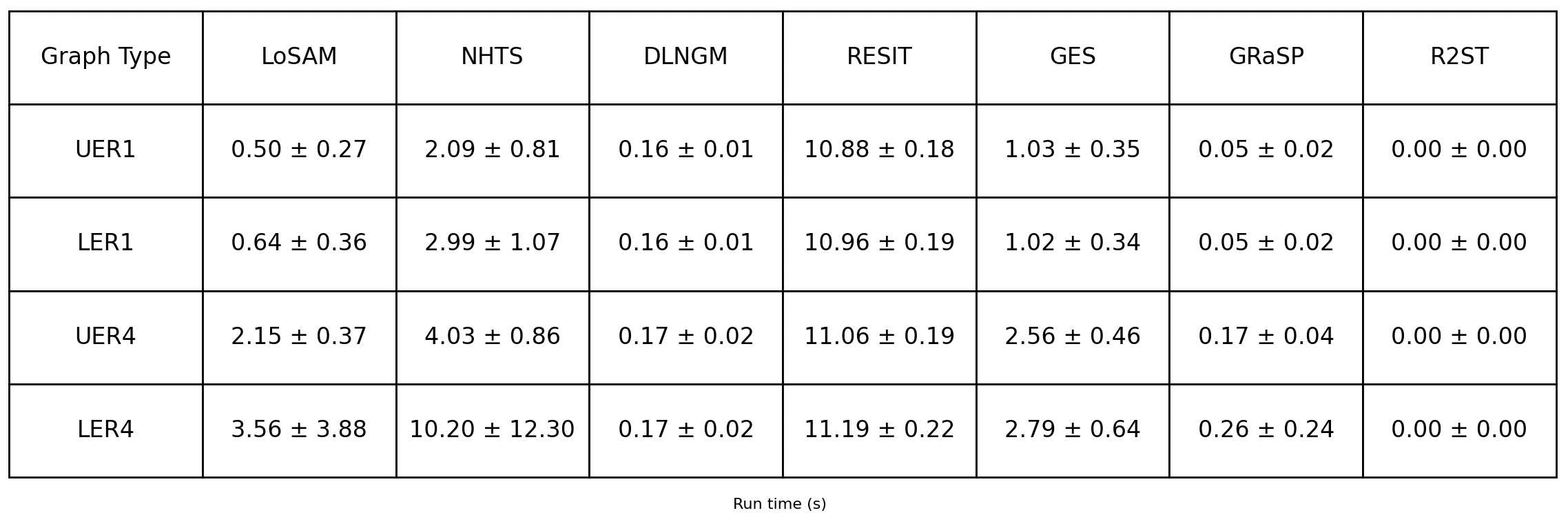
Figure 5: Runtimes for topological sorts on ANM with linear mechanisms. See Column 1 of Figure 4.

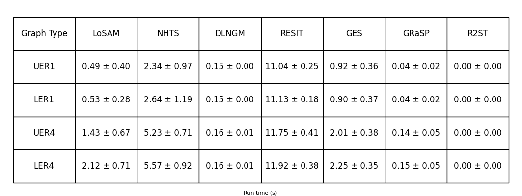
Figure 6: Runtimes for topological sorts on ANM with mixed mechanisms. See Column 2 of Figure 4.

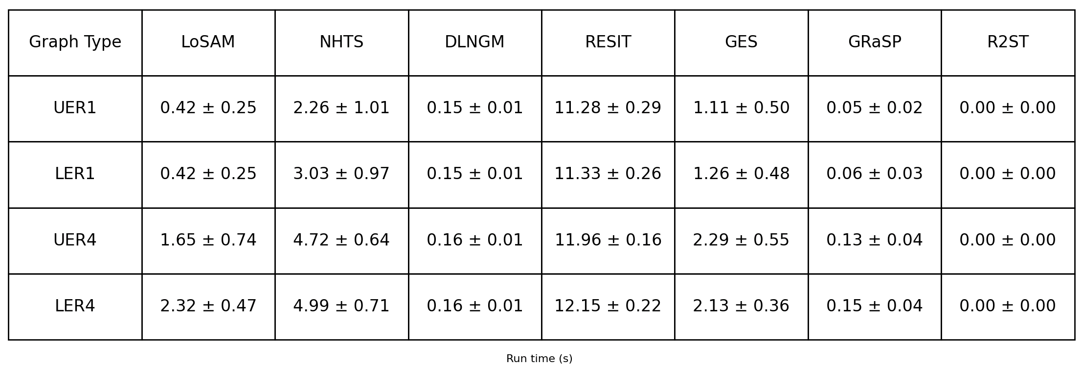
Figure 7: Runtimes for topological sorts on ANM with nonlinear mechanisms. See Column 3 of Figure 4.

Appendix H ALGORITHM WALKTHROUGHS

In this section we walk-through LoSAM and LoSAM-UC on exemplary DAGs.

H.1 LoSAM

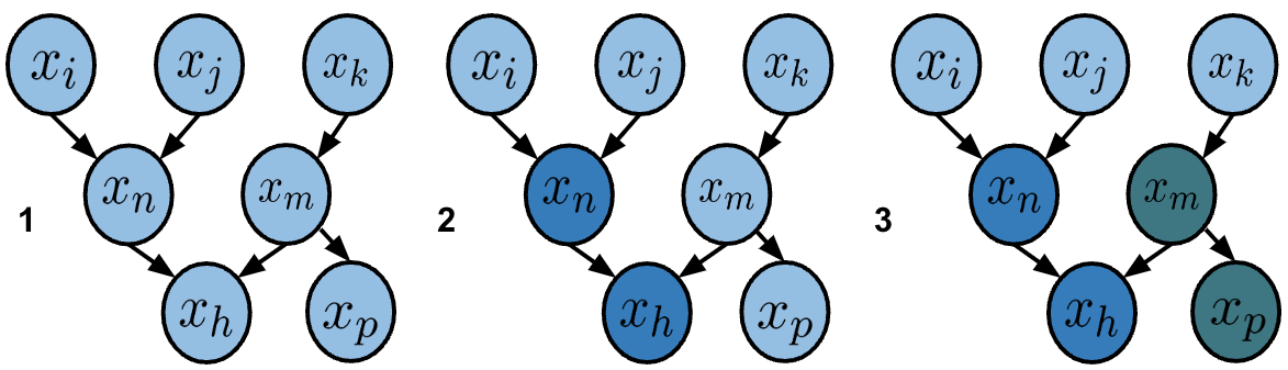
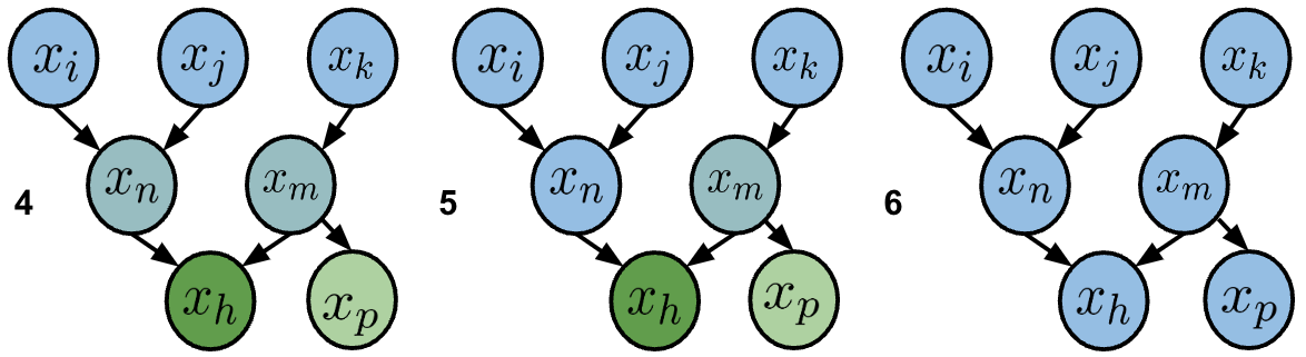
Figure 8: LoSAM walkthrough on example DAG.

Subfigure 1 of Figure 8 illustrates the example causal graph from which data is generated. Now, we walk through how LoSAM would obtain a topological sort of this DAG. In Stage 1 Root Finder, $x_{n},x_{h}$ are identified as MRDs and are pruned (subfigure 2). Then, $x_{i},x_{j}$ are recovered as roots, as they are independent of $x_{k},x_{m},x_{p}$. Then, in Stage 2, $x_{m},x_{p}$ are pruned as they are not identified as ancestors of any vertices, while $x_{k}$ is (subfigure 3). We therefore recover $x_{i},x_{j},x_{k}$ as roots. Subfigure 4 illustrates the decomposition of the graph into roots ($x_{i},x_{j},x_{k}$), VCs ($x_{n},x_{m}$), a ND $x_{h}$ and an LD ($x_{p}$). In Stage 1 of Sort Finder, $x_{p}$ is pruned from $U=\{x_{n},x_{m},x_{p},x_{h}\}$ as it as an LD. Then, $x_{n}$ is determined as a VC, as a minimizer of the test statistic $t^{*}$ (subfigure 5), and is sorted. This is again repeated 3 more times to sort all of $U$ (subfigure 6); therefore, LoSAM correctly obtains a valid sort $\pi$.

H.2 LoSAM-UC

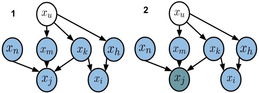
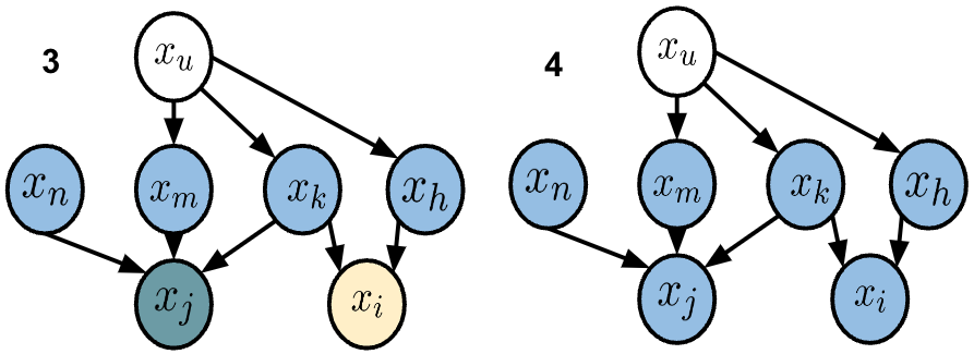
Figure 9: LoSAM walkthrough on example DAG.

Subfigure 1 of Figure 9 illustrates the example causal graph from which data is generated, where $x_{u}$ is unobserved. In Stage 1 of LoSAM-UV, $x_{j}$ is identified as a MRD-I and is pruned (subfigure 2). Then, $x_{m}$ is found as a proxy of $x_{k},x_{h}$, and therefore we identify that $x_{k}\perp\!\!\!\perp x_{h}$ given some unobserved confounder, and therefore $x_{i}$ induces a VP between $x_{k},x_{h}$ as a MRD-N. After pruning $x_{i},x_{j}$, we identify $x_{n}$ as a root, independent of $x_{m},x_{j},x_{h}$. In Stage 2, we confirm that $x_{m},x_{k},x_{h}$ are roots (subfigure 4) by recovering independent residuals from every bivariate regression. Using the discovered roots, in Stage 3 Sort Finder recovers a valid topological sort $\pi$.

Appendix I EXAMPLE EXPLANATIONS

I.1 FAILURE-MODES OF LoSAM

In this section, we detail how LoSAM, a method designed for fully observed models, may fail to accurately recover the true topological sort when unobserved variables are present. We detail how the Root Finder may fail in multiple different stages of the subroutine (Algorithm 1) to prune non-roots from roots.

Figure 10: LoSAM Failure Mode 1.

First, we use the exemplary DAG provided in Figure 10, where there exists an unobserved confounder $x_{u}$ between roots $x_{m},x_{k},x_{h}$. Note that in Stage 1 of Root Finder, pairwise independence tests are leveraged to prune all MRDs. However, although $x_{i},x_{j}$ are both MRDs with respect to observed variables, $x_{i}$ is not pruned due to $x_{u}$ confounding both root ancestors $x_{k},x_{h}$. Then, note that in Stage 2 of Root Finder, pairwise regression is leveraged to identify the root superset $W$, which consists of those vertices identified as ancestors by the Ancestor-Descendant Test. However, for $x_{k},x_{h}$ to be identified, this requires that there is an independent residual produced when $x_{i}$ is regressed onto $x_{k}$, and likewise when $x_{i}$ is regressed onto $x_{h}$. Suppose $x_{i}=x_{k}x_{h}+\varepsilon_{i}$; then, no independent residual is recovered from any pairwise regression, thus $x_{i}$ is not pruned from $W$, and therefore LoSAM fails to distinguish roots from non-roots.

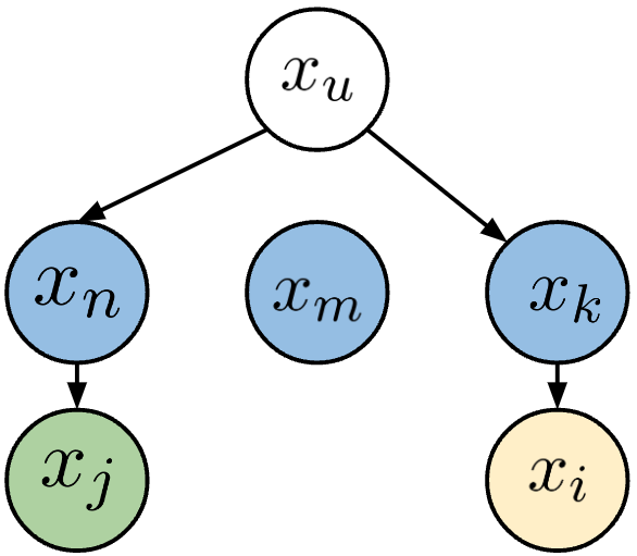
Figure 11: LoSAM Failure Mode 2.

Second, we use the exemplary DAG provided in Figure 11, where there exists an unobserved confounder $x_{u}$ between roots $x_{n},x_{k}$. Note that Stage 1 of Root Finder successfully prunes all MRDs, given that none exist in the DAG. Note that the root superset $W=\{x_{n},x_{k}\}$ is correctly identified; however, the conditional independence approach fails to identify $x_{n},x_{k}\in W$ as roots. Note that $x_{n}\not\!\perp\!\!\!\perp x_{k}$ due to the latent confounder $x_{u}$, and that $x_{n},x_{k}$ do d-separate $x_{j},x_{i}$ from each other: we have $x_{j}\perp\!\!\!\perp x_{k}|x_{n},x_{i}\perp\!\!\!\perp x_{n}|x_{k}$. This means that $x_{n},x_{k}$ cannot be pruned from $W$, and therefore LoSAM fails to distinguish roots from non-roots.

I.2 PROXY VARIABLES

In this section we further explain how the procedure provided by Liu et al., (2024) leverages proxy variables to recover the existence of causal relationships under latent confounding, allowing us to recover independence relations between roots.

Figure 12: Classic Proxy Variable Illustration.

Figure 12 illustrates the general case where $x_{h}$ is a proxy variable for $x_{m},x_{k}$, which are latently confounded by the unobserved variable $x_{u}$. It is unknown whether a direct causal relationship between $x_{m},x_{k}$ exists, i.e., whether $x_{m}\perp\!\!\!\perp x_{k}|x_{u}$. Importantly, $x_{h}$ is a descendent of the latent confounder $x_{u}$, but $x_{h}\perp\!\!\!\perp x_{m}|x_{u},x_{h}\perp\!\!\!\perp x_{k}|x_{u}$; this dependence structure naturally arises when latent confounding exists between multiple roots.

Suppose that there exists no edge between $x_{m},x_{k}$, i.e., $x_{m}\perp\!\!\!\perp x_{k}$. A normal independence test between $x_{m},x_{k}$ would find that $x_{m}\not\!\perp\!\!\!\perp x_{k}$. However, the procedure in Liu et al., (2024) leverages the proxy $x_{h}$ to identify that $x_{m}\perp\!\!\!\perp x_{k}|x_{u}$, without having observed $x_{u}$. This means that if a proxy for two latently confounded roots exist, one can recover the independence of the two roots; this allows us to identify all possible VPs, enabling the pruning of MRD-Ns.

I.3 LEMMA 3.3 FAILURE MODE

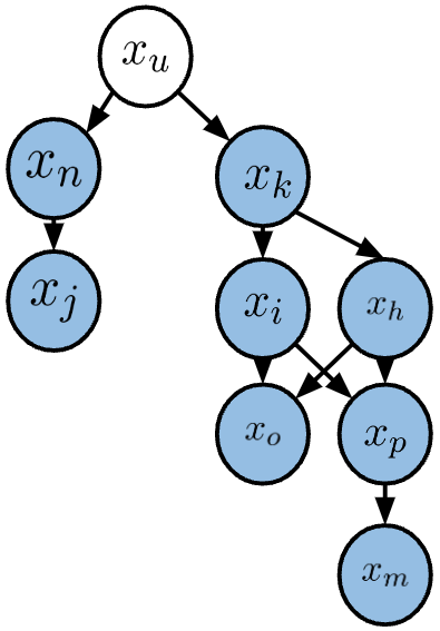
Figure 13: Exemplary DAG, to highlight where Lemma 3.3 may fail.

In this section we formalize how Lemma 3.3 may fail when latent confounders between roots exist, walking through a specific example DAG, illustrated in Figure 13.

Observe Figure 13, where $x_{u}$ is unobserved. As there are no MRDs, Stage 1 of Root Finder prunes no vertices and identifies no roots. In Stage 2, note that $x_{n}$ must be identified $\in\text{An}(x_{j})$, $x_{k}$ must be identified $\in\text{An}(x_{i}),\in\text{An}(x_{h})$, $x_{p}$ must be identified $\in\text{An}(x_{m})$. Therefore, $W=\{x_{n},x_{k},x_{p}\}$. Note that by Lemma 3.3 a vertex $x\in W$, is a root iff it fails to d-separate at least one of its identified descendants from every vertex it is dependent on. As expected, $x_{p}$ d-separates its only descendant $x_{m}$ from both $x_{n}$ and $x_{k}$, so it cannot be a root. However note that $x_{k}$ d-separates both its identified descendants $x_{i}$ or $x_{h}$ from $x_{n}$, while $x_{n}$ d-separates its only identified descendant $x_{j}$ from $x_{k}$ and $x_{p}$. The issue is that $x_{u}$ induces an active backdoor path between $x_{n},x_{k}$; by making roots dependent, we lose guaranteed asymmetry between roots and non-roots when considering vertices that are mutually dependent. Therefore, we are unable to prune any of $x_{n},x_{k},x_{p}$ as non-roots via Lemma 3.3 in Root Stage 2 of Root Finder.

Appendix J LIMITATIONS

We note that the standard approach in the causal discovery literature to assess a method’s finite sample performance is to evaluate the method on synthetically generated data (Reisach et al.,, 2021). This is because causal ground truth is incredibly rare, as it requires real-world experiments (Faller et al.,, 2024); these experiments can expensive, potentially unethical, but most importantly are often infeasible or ill defined (Spirtes and Scheines,, 2004). This lack of substantial real-world benchmark datasets is important because key assumptions that are used to generate synthetic data, which discovery methods rely on (such as additive noise, faithfulness, and causal sufficiency), may be violated in practice (Faller et al.,, 2024). Therefore we caution that experimental results on synthetic data should be interpreted as a demonstration of a method’s theoretical performance on somewhat idealized data, which may not reflect measurements from real-world settings where assumptions critical to the method are not met.

Appendix K ASSET INFORMATION

GES and GRaSP were imported from the causal-learn search package. DirectLiNGAM and RESIT were imported from the lingam package. $R^{2}-$sort was imported from the CausalDisco package. NHTS and LoSAM were implemented using the kernel ridge regression function from the Sklearn package, used kernel-based independence tests from the causal-learn package, and a mutual information estimator from the npeet package. All assets used have a CC-BY 4.0 license. See file named ‘aistats2025_topological_sort_experiments’ for further details.

References

- Bühlmann et al., (2014) Bühlmann, P., Peters, J., and Ernest, J. (2014). CAM: Causal additive models, high-dimensional order search and penalized regression. The Annals of Statistics, 42(6). arXiv:1310.1533 [cs, stat].
- Cheng et al., (2023) Cheng, D., Li, J., Liu, L., Yu, K., Duy Le, T., and Liu, J. (2023). Toward Unique and Unbiased Causal Effect Estimation From Data With Hidden Variables. IEEE Transactions on Neural Networks and Learning Systems, 34(9):6108–6120.
- Chickering, (2002) Chickering, D. M. (2002). Learning Equivalence Classes of Bayesian Network Structures.
- Erdos and Renyi, (1960) Erdos, P. and Renyi, A. (1960). On the evolution of random graphs.
- Faller et al., (2024) Faller, P., Vankadara, L., Mastakouri, A., Locatello, F., and Janzing, D. (2024). Self-compatibility: Evaluating causal discovery without ground truth. International Conference on Artifical Intellgience and Statistics.
- Glymour et al., (2019) Glymour, C., Zhang, K., and Spirtes, P. (2019). Review of Causal Discovery Methods Based on Graphical Models. Frontiers in Genetics, 10:524.
- Hiremath et al., (2024) Hiremath, S., Maasch, J., Gao, M., Ghosal, P., and Gan, K. (2024). Hybrid top-down global causal discovery with local search for linear and nonlinear additive noise models. To appear in NeurIPS 2024. https://arxiv.org/abs/2405.14496.
- Hoyer and Hyttinen, (2009) Hoyer, P. O. and Hyttinen, A. (2009). Bayesian discovery of linear acyclic causal models. In Proceedings of the 25th Conference on Uncertainty in Artificial Intelligence.
- Hoyer et al., (2008) Hoyer, P. O., Shimizu, S., Kerminen, A. J., and Palviainen, M. (2008). Estimation of causal effects using linear non-Gaussian causal models with hidden variables. International Journal of Approximate Reasoning, 49(2):362–378.
- Ke et al., (2023) Ke, N., Chiappa, S., Wang, J., Bornschein, J., Goyal, A., Rey, M., Weber, T., Botvinick, M., Mozer, M., and Rezende, D. (2023). Learning to induce causal structure. International Conference on Learning Representations.
- Kraskov et al., (2004) Kraskov, A., Stögbauer, H., and Grassberger, P. (2004). Estimating mutual information. Physical Review E, 69(6):066138.
- Kuroki and Pearl, (2014) Kuroki, M. and Pearl, J. (2014). Measurement bias and effect restoration in causal inference.
- Lam et al., (2022) Lam, W.-Y., Andrews, B., and Ramsey, J. (2022). Greedy Relaxations of the Sparsest Permutation Algorithm.
- Lippe et al., (2022) Lippe, P., Cohen, T., and Gavves, E. (2022). Efficient neural causal discovery without acyclicity constraints. International Conference on Learning Representations.
- Liu et al., (2024) Liu, M., Sun, X., Qiao, Y., and Wang, Y. (2024). Causal discovery via conditional independence testing with proxy variables.
- Maasch et al., (2024) Maasch, J., Pan, W., Gupta, S., Kuleshov, V., Gan, K., and Wang, F. (2024). Local discovery by partitioning: Polynomial-time causal discovery around exposure-outcome pairs. In Proceedings of the 40th Conference on Uncertainy in Artificial Intelligence.
- Maeda and Shimizu, (2020) Maeda, T. N. and Shimizu, S. (2020). RCD: Repetitive causal discovery of linear non-Gaussian acyclic models with latent confounders. In Proceedings of the 23rd International Conference on Artificial Intelligence and Statistics (AISTATS).
- Maeda and Shimizu, (2021) Maeda, T. N. and Shimizu, S. (2021). Causal Additive Models with Unobserved Variables. In Proceedings of the Thirty-Seventh Conference on Uncertainty in Artificial Intelligence, page 10.
- Miao et al., (2018) Miao, W., Geng, Z., and Tchetgen Tchetgen, E. (2018). Identifying causal effects with proxy variables of an unmeasured confounder.
- (20) Montagna, F., Mastakouri, A. A., Eulig, E., Noceti, N., Rosasco, L., Janzing, D., Aragam, B., and Locatello, F. (2023a). Assumption violations in causal discovery and the robustness of score matching. In 37th Conference on Neural Information Processing Systems.
- (21) Montagna, F., Noceti, N., Rosasco, L., Zhang, K., and Locatello, F. (2023b). Causal Discovery with Score Matching on Additive Models with Arbitrary Noise. In Proceedings of the 2nd Conference on Causal Learning and Reasoning. arXiv. arXiv:2304.03265 [cs, stat].
- Pearl et al., (2016) Pearl, J., Glymour, M., and Jewell, N. P. (2016). Causal inference in statistics: a primer. Wiley, Chichester, West Sussex.
- Peters et al., (2014) Peters, J., Mooij, J., Janzing, D., and Schölkopf, B. (2014). Causal Discovery with Continuous Additive Noise Models. arXiv:1309.6779 [stat].
- Reisach et al., (2021) Reisach, A., Seiler, C., and Weichwald, S. (2021). Beware of the simulated dag! causal discovery benchmarks may be easy to game. Advances in Neural Information Processing Systems, 34:27772–27784.
- Reisach et al., (2023) Reisach, A. G., Tami, M., Seiler, C., Chambaz, A., and Weichwald, S. (2023). A Scale-Invariant Sorting Criterion to Find a Causal Order in Additive Noise Models. In 37th Conference on Neural Information Processing Systems. arXiv. arXiv:2303.18211 [cs, stat].
- Rolland et al., (2022) Rolland, P., Cevher, V., Kleindessner, M., Russel, C., Scholkopf, B., Janzing, D., and Locatello, F. (2022). Score Matching Enables Causal Discovery of Nonlinear Additive Noise Models. In Proceedings of the 39 th International Conference on Machine Learning.
- Shah et al., (2024) Shah, A., Shanmugam, K., and Kocaoglu, M. (2024). Front-door adjustment beyond markov equivalence with limited graph knowledge. Advances in Neural Information Processing Systems, 36.
- Shimizu et al., (2006) Shimizu, S., Hoyer, P. O., Hyvarinen, A., and Kerminen, A. (2006). A Linear Non-Gaussian Acyclic Model for Causal Discovery. Journal of Machine Learning Research, 7:2003–2030.
- Shimizu et al., (2011) Shimizu, S., Inazumi, T., Sogawa, Y., Hyvarinen, A., Kawahara, Y., Washio, T., Hoyer, P. O., Bollen, K., and Hoyer, P. (2011). Directlingam: A direct method for learning a linear non-gaussian structural equation model. Journal of Machine Learning Research-JMLR, 12(Apr):1225–1248.
- Spirtes, (2001) Spirtes, P. (2001). An Anytime Algorithm for Causal Inference. In Proceedings of the Eighth International Workshop on Artificial Intelligence and Statistics, volume R3, pages 278–285. PMLR.
- Spirtes et al., (2000) Spirtes, P., Glymour, C., and Scheines, R. (2000). Causation, Prediction, and Search, volume 81 of Lecture Notes in Statistics. Springer New York, New York, NY.
- Spirtes and Scheines, (2004) Spirtes, P. and Scheines, R. (2004). Causal inference of ambiguous manipulations. Philosophy of Science.
- Spirtes and Zhang, (2016) Spirtes, P. and Zhang, K. (2016). Causal discovery and inference: concepts and recent methodological advances. Applied Informatics, 3(1):3.
- Zhang and Hyvarinen, (2009) Zhang, K. and Hyvarinen, A. (2009). On the Identifiability of the Post-Nonlinear Causal Model. Uncertainty in Artificial Intelligence.