Identification and modelling of optically thin inverse Compton scattering in the prompt emission of GRB131014A

Abstract

The mechanism responsible for the prompt gamma-ray emission of a gamma-ray burst continues to remain an enigma. The detailed analysis of the spectrum of GRB 131014A observed by the Fermi gamma ray burst monitor and Large Area Telescope has revealed an unconventional spectral shape that significantly deviates from the typical Band function. The spectrum exhibits three distinctive breaks and an extended power law at higher energies. Furthermore, the lower end of the spectrum aligns with power-law indices greater than -0.5, and in the brightest region of the burst, these values approach +1. The lowest spectral break is thereby found to be consistent with a blackbody. These observed spectral characteristics strongly suggest the radiation process to be inverse Compton scattering in an optically thin region. Applying the empirical fit parameters for physical modeling, we find that the kinetic energy of the GRB jet of bulk Lorentz factor, $\Gamma\sim 400$, gets dissipated just above the photosphere, approximately at a radius of $\sim 10^{14}$ cm. The electrons involved in this process are accelerated to a power-law index of $\delta=-1.5$, and the minimum electron Lorentz factor, $\gamma_{min}$, is approximately $3$. In summary, this study provides a comprehensive identification and detailed modeling of optically thin inverse Compton scattering in the prompt emission of GRB 131014A.

1 Introduction

Gamma ray bursts are the brightest explosive transients occurring in the distant cosmos. The origin of the intense gamma rays produced during the event is still debated. The uniqueness and non-repeating nature of GRB along with its wide variety of emission light curves makes it challenging to develop a generic radiation model for GRBs.

Within the classical fireball model scenario (Mészáros, 2006; Kumar & Zhang, 2015; Iyyani, 2018), the observed gamma ray emission is anticipated to be produced from the photosphere and in the optically thin regions above the photosphere. The high optical depth leading to the numerous scatterings of the radiation with the plasma results in thermalised emission from the photosphere. However, the kinetic energy dissipated in the site above the photosphere leads to relativistic shocks wherein the accelerated electrons cool via various non-thermal radiation processes. The competing non-thermal emission mechanisms are synchrotron emission (Rees & Meszaros, 1992; Tavani, 1996; Sari & Piran, 1997; Beniamini & Giannios, 2017; Beniamini et al., 2018) and Inverse Compton scattering (ICS) (Panaitescu & Mészáros, 2000; Stern & Poutanen, 2004; Pe’er & Waxman, 2004; Nakar et al., 2009; Ahlgren et al., 2015; Iyyani et al., 2015).

Synchrotron emission has long been favored as a model to explain non-thermal emissions in astrophysical phenomena. While it is widely accepted for producing non-thermal spectral shapes, straightforward synchrotron emission models struggle to account for the prompt emission spectra of GRBs. These challenges include hard low-energy spectral slopes, a narrow range of spectral peak energies (Iyyani, 2018), and the majority of GRB spectra being consistent with slow-cooled synchrotron emission models have lower radiation efficiencies, while, the fast-cooled synchrotron emission, is radiation-efficient, however, produces broad spectral peaks that are found to be inconsistent with the data (Burgess et al., 2014) etc. Nonetheless, several modified versions of synchrotron emission scenarios have been proposed to address these limitations (Dermer et al., 2000; Asano et al., 2009; Uhm & Zhang, 2014; Beniamini et al., 2018; Burgess et al., 2019).

The alternative non-thermal emission process that has been actively studied is inverse Compton scattering under various scenarios such as subphotospheric dissipation (Ghisellini & Celotti, 1999; Iyyani et al., 2015; Ahlgren et al., 2015) and synchrotron self Compton emission models in context of prompt emission (Granot et al., 2000; Lloyd & Petrosian, 2000; Stern & Poutanen, 2004; Zhang et al., 2019) and afterglow emissions (Abdalla et al., 2019; Derishev & Piran, 2019; Wang et al., 2019; Sari & Esin, 2001; Zhang et al., 2020). A significant limitation in this model, as highlighted by Piran et al. 2009, arises when the seed photons are considered at lower energies, such as optical or infrared. If the observed gamma-ray emission is considered to result from the inverse Compton upscattering of these seed photons, it implies a substantial amplification or, in other words, a high average electron Lorentz factor. This, in turn, would lead to higher order scatterings with emissions peaking at TeV energies, ultimately straining the energy budget of a GRB. However, this issue can be addressed if the seed emission originates at relatively higher energies such that the amplification reduces. Moreover, if the upscattered photons surpass the energy threshold for pair production, this can subsequently reduce the average electron Lorentz factor, thereby suppressing the higher-order scatterings (Piran et al., 2009).

In this study, we characterize an uncommon spectral shape with multiple spectral breaks in GRB 131014A through a comprehensive spectral analysis. Additionally, we model the observed spectrum using the optically thin inverse Compton scattering radiation mechanism. In sections 2 and 3, we describe the observations and the spectral analysis respectively. In section 4, we present the physical modelling to derive the physical scenario of the observed spectra. We present the discussions on the observed spectral properties and its physical interpretation in section 5 and finally conclude in section 6.

2 Observations

On 14 October 2013, multiple space satellites including Fermi Gamma-ray space telescope (Fitzpatrick & Xiong, 2013; Desiante et al., 2013), Konus Wind (Golenetskii et al., 2013) and Suzaku Wide-band All-sky Monitor (WAM; (Kawano et al., 2013)) triggered on the GRB131014A. The burst was localised in the sky at RA = $100.29^{\circ}$ and Dec = $-19.13^{\circ}$ with nearly $53^{\prime}$ uncertainty (Hurley et al., 2013). Nearly 12 hours post the trigger, the target of opportunity (ToO) observations carried out by Swift X-Ray Telescope (XRT) resulted in a detection of a fading X- ray source (Amaral-Rogers et al., 2013). An optical transient tentatively linked to this event was also later reported (Schulze et al., 2013; Kann et al., 2013; Swenson & Amaral-Rogers, 2013). However, there was no robust redshift measurement made for the burst.

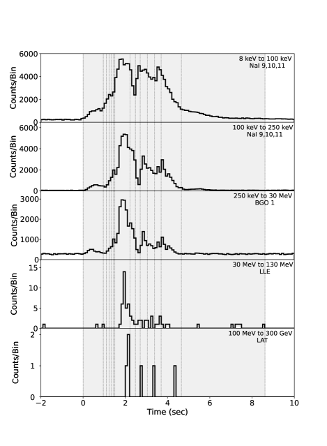
Figure 1: The multi-panel light curve (black solid line) of GRB 131014A with $0.1$ s binning, as observed across different energy ranges of NaI(9,10,11), BGO 1 and LAT detectors is shown. The shaded grey area represents the duration of the burst studied for time resolved spectral analysis. Additionally, the dotted vertical lines depict the time resolved intervals obtained from Bayesian block binning.

At 05:09:00.20 UT ($T_{0}$), the GRB triggered the two instruments aboard the Fermi spacecraft: the Gamma Ray Burst Monitor (GBM, covering 8 keV to 40 MeV) and the Large Area Telescope (LAT, spanning 30 MeV to 300 GeV). The burst displayed a complex, multi-pulsed light curve, depicted in Figure 1, illustrating its activity across increasing energy levels. The lightcurve includes observations of various detectors aboard GBM, including sodium iodide (NaI) covering 8 keV - 100 keV and 100 keV - 250 keV, as well as bismuth germanate (BGO) covering 250 keV - 30 MeV. Additionally, data from the LAT Low Energy (LLE, 30 MeV - 130 MeV) and LAT ($>100,\rm MeV$) detectors are included. The LLE and LAT emission commenced at $T_{0}+0.06\,s$ and $T_{0}+2.16\,s$ respectively. The LAT observations extended until $T_{0}+15\,s$ and detected a total of $31$ photons with energies exceeding $100\,\rm MeV$, with the highest photon energy recorded at $1.8\,\rm GeV$ occurring at $T_{0}+14\,s$ (Desiante et al., 2013). The burst had a duration of $T_{90}=3.2\pm 0.09\,s$ where $T_{90}$ represents the time interval during which $90\%$ of the burst fluence is measured. The burst recorded an energy fluence of $1.98\times 10^{-4}\,\rm erg\,cm^{-2}$, positioning it as the second most luminous among the shorter duration GRBs observed by Fermi with $T_{90}\leq 5\,s$.

3 Spectral Analysis

The spectral analyses were conducted using the Multi-Mission Maximum Likelihood (3ML, (Burgess et al., 2021)) package. The analysis included Fermi data from the three brightest NaI detectors, NaI 9, 10 and 11 with source angles $<60^{\circ}$ (Gruber et al., 2014) along with BGO 1 and LAT detectors providing a spectral coverage from $8$ keV to several GeV. In case of NaI detectors, data in the energy range 30 keV to 40 keV corresponding to the iodine-K edge were excluded, in addition, to those in the extreme edges such as those below 8 keV and those above 900 keV. For BGO, LAT-LLE and LAT ($>100MeV$) detectors, the data within the energy ranges 250 keV - 10 MeV, 30 MeV - 100 MeV and 100 MeV - 2 GeV were used respectively. The burst interval from 0 to 8.6 s where chosen for both the time integrated and time resolved analyses. The background was modelled using a polynomial function best fitted to data in the intervals pre ($T_{0}-20$s to $T_{0}-2$s) and post ($T_{0}+20$s to $T_{0}+30$s) the burst duration. The technique of maximum likelihood estimate was employed for estimating the model parameters while the Akaike Information Criterion (AIC) was used for the model selection.

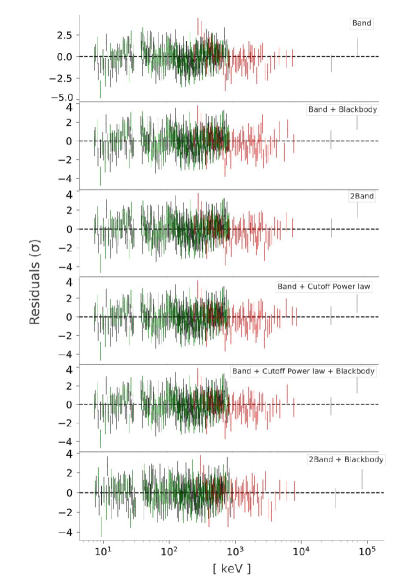
Figure 2: The residuals obtained for the spectral analysis using different models: Band, Band + blackbody, 2Band, Band + Cutoff power law, Band + Cutoff power law + blackbody, 2Band + blackbody, fitted to the data of the time interval [3.04s, 3.38s], are shown in ascending order from the upper to the lower panels, respectively.

The spectral analysis allows to identify and characterise the shape of the spectrum and subsequently the emission mechanism. Given the dynamic nature of GRB emissions, evident from their intricate light curves, employing the time-resolved spectroscopy becomes crucial. This approach enables us to identify the underlying instantaneous spectral shape, which might otherwise get smeared, leading to lose of precise spectral information when modeled over the entire duration during time-integrated analysis. Furthermore, in order to investigate the temporal evolution of the spectrum, a time-resolved spectral analysis of the burst was conducted. The time intervals of the analysis were determined using the Bayesian block binning method (Scargle, 1998) which resulted in 14 time bins. A detailed time resolved spectroscopy was carried out for the burst duration from 0 s to 8.6 s.

The underlying instantaneous spectral shape of the burst radiation can be best identified in the time resolved brightest bins with higher number of counts. Thus, the spectral analysis was initiated in the time intervals during the bright regions of the burst assuring enough number of photon counts for analysis. The joint spectral analysis including data from GBM and LAT detectors requires an effective area correction to be incorporated. The spectral data was initially modelled using the conventional models such as the Band function (Band et al., 1993) (Band) alone and in combination with a blackbody (Band + BB) (Axelsson et al., 2012; Iyyani et al., 2013). In addition, several intermediate complexity models such as ’Smoothly Broken Power Law’, ’Blackbody + Band $\times$ High Energy Cutoff’, ’Cutoff Power Law + Power Law’, ’Cutoff Power Law (CPL) + Blackbody’, ’Band + Cutoff Power Law’, ’Band + Cutoff Power Law + Power Law’, ’Band + Cutoff Power Law + Blackbody’ and a few more, were also tried for spectral modelling. However, these models resulted in poor fits with wavy residuals, often with unconstrained parameters, and occasionally with spectral components switching places between consecutive fits leading to inconsistent temporal evolution of the parameters. This strongly suggested that the spectrum has a more complicated shape.

A significant improvement in fitting was observed by adding an extra Band function to the Band + BB model, resulting in the most random structure of the residuals. We note that while the Band + CPL + BB model is an equally good fit in some time intervals, it results in poor fits in others. Despite having one fewer free parameter compared to the 2Bands + BB model, the Band model is more flexible than the Cutoff Power Law, allowing it to more accurately capture the spectral shapes of other time-resolved intervals as the spectrum evolves. Thus, the 2Bands + BB model is found to better capture the overall spectral evolution (see Table 1 in Appendix A).

By choosing 2 Bands + BB as the best fit model, the effective area correction factors i.e, the normalisation offsets of the detectors were estimated by fitting the data with this spectral model multiplied by a constant of normalisation for each instrument. The constant of the brightest NaI detector i.e NaI 10 was frozen at unity while that of all other detectors were kept free. The effective area correction factors for the various detectors were found as follows: $1\pm 0.009$, $1\pm 0.009$, $1.03\pm 0.015$ and $1.8\pm 0.6$ for NaI 9, NaI 11, BGO 1 and LLE respectively. Including the effective correction factors, the best fit model, 2 Bands + BB model brought about an improvement in the AIC statistics by $\Delta\,\rm AIC=49$, $\Delta\,\rm AIC=28$ and $\Delta\,\rm AIC=16$ with respect to the Band function fit alone, Band + BB and Band + CPL + BB respectively in the time interval [3.04s, 3.38s]. For comparison between the various spectral model fits, the residuals obtained in the case of Band only, Band + BB, 2 Bands, Band + CPL, Band + CPL + BB and 2 Bands + BB for the analysis of the time interval [3.04s, 3.38s], where the most significant improvement in $\Delta\,\rm AIC$ is obtained, are shown in the Figure 2. We note that the residuals follow a more random behaviour with minimal waviness in the case of 2 Bands + BB.

We further note that during the time-resolved analysis, in the initial time bins from 0 s to 1.49 s, the blackbody component could not be well-constrained, making 2Bands the best fit model. Although ’Band + Cutoff Power Law’ was sometimes an equally good fit, the overall spectral shapes remained unchanged. For continuity in modeling throughout the burst emission, we chose 2Bands as the best fit model in the initial bins where the blackbody component could not be constrained. This choice also ensured the continuity of the spectral model and consistent temporal evolution of the parameters. The identified shape of the overall spectrum (green solid line) of GRB131014A as in the $\nu F_{\nu}$ space in the regions before and after $1.49s$ are shown in Figure 3(a) and 3(b) respectively. The overall spectral shape exhibits multiple peaks/ breaks in the spectrum.

Furthermore, the time-integrated spectrum spanning from 0 to 8.6 s was also found to be well modelled using 2 Bands + BB yielding a significant improvement in the statistic by reducing the AIC by $229$, $79$ and $30$ with respect to the Band function only, Band + BB and Band + CPL + BB fits respectively. The obtained fit parameters of the best fit model is reported in the Table 1 in Appendix A. Thus, the spectral analysis of the burst reveals a unique overall spectral shape, distinct from the conventional GRB spectral shapes like the Band function or Band + Blackbody. The burst fluence is estimated to be 5$\times$$10^{-4}$ $erg/cm^{2}$ which corresponds to a total burst energy of 2.7 $\times$$10^{55}$ $erg$ assuming a redshift $z=2.12$ , radiation efficiency (1/Y) of 0.67 (Racusin et al., 2011) and the standard $\Lambda_{CDM}$ cosmology along with the cosmological parameters, $H_{0}=67.4\pm 0.5\,km\,s^{-1}\,Mpc^{-1}$, $\Omega_{m}=0.315$ and $\Omega_{vac}=0.685$ (Aghanim et al., 2020).

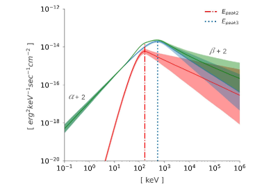
(a) Time interval : 1.34 s - 1.44 s

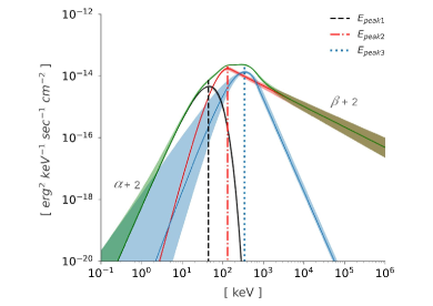
(b) Time interval : 3.04 s - 3.38 s

Figure 3: The spectral shape of the burst spectrum characterised by the best fit empirical model: (a) 2 Bands in time intervals less than $1.49s$ and (b) 2 Bands+ Blackbody in the time intervals above $1.49s$ are shown in the above $\nu\,F_{\nu}$ plots in green solid line. The shaded green region signifies the $68\%$ confidence interval of the overall model. The resulting shape of the spectrum is defined by the parameters: $\alpha$ and $\beta$ represent the low and high energy asymptotic power law indices respectively, while the three $\nu\,F_{\nu}$ peaks denoted by the $E_{peak1}$, $E_{peak2}$ and $E_{peak3}$ are marked by black (dashed), red (dash dotted) and blue (dotted) lines respectively. The individual spectral components of the model are also shown in black (Blackbody), red (Band₁) and blue (Band₂) solid lines along with their $68\%$ confidence intervals with same shaded colour.

3.1 Best fit model: 2 Bands + Blackbody

The multiple additive components composing the spectral model 2 Bands + BB (Figure 3) essentially captures the complex shape of the overall spectrum with the multiple breaks and the asymptotic power law behaviours observed both at the lower and higher energies. It is noted that all the parameters of the individual composing components are thereby are not essential eventually to characterise the overall net spectral shape. Therefore, we parameterise the obtained overall spectral shape in terms of the following parameters:

• $E_{peak1}$: The first spectral peak which is modelled by the blackbody component is referred to as $E_{peak1}$ which is around a few tens of keV. $E_{peak1}$ corresponds to the $\nu F_{\nu}$ peak of the blackbody fit.

• $E_{peak2}$: The second spectral peak modelled by one of the Band functions is referred to as $E_{peak2}$ which is around a hundred keV.

• $E_{peak3}$: The third spectral peak modelled by the second Band function is referred to as $E_{peak3}$ with values around a few hundreds of keV.

• $\alpha$: The low energy spectral index of the asymptotic power-law obtained below the spectral peak, $E_{peak1}$.

• $\beta$: The high energy spectral index of the asymptotic power-law obtained above the spectral peak, $E_{peak3}$.

The $\alpha$ and $\beta$ are determined by fitting a power law function to the low energy asymptotic part (below $E_{peak1}$) and the high energy asymptotic part (above $E_{peak3}$) of the photon flux plot of the overall spectral shape, respectively. The $68\%$ confidence interval errors for these indices were derived by fitting the power law function to the low and high energy asymptotic parts of the upper and lower bound curves of the $68\%$ region of the overall photon flux spectral shape, respectively. These parameters are depicted on the $\nu F_{\nu}$ plot in the Figure 3.

Furthermore, it is interesting to note that in addition to the spectral peaks mentioned above, the asymptotic power-law in the higher energies creates an extra break. In other words, the asymptotic behaviour of the higher energy spectrum significantly deviates from the turnover predicted by the $E_{peak3}$ in the higher end. In the following subsection, the temporal evolution of these five parameters along with the energy fluxes are presented.

3.2 Spectral analysis results

The evolution of the spectral parameters of the 2Bands+BB model as characterised in the preceding section, obtained via the time resolved analysis is presented in the Figure 4. The parameter $\alpha$, which represents the low-energy asymptotic power-law index, tends to stay predominantly above $-0.5$ and, in some instances, even reaches values close to $+1$ (Figure 4a). As the burst progresses and the emission is integrated over longer time intervals particularly towards the end, $\alpha$ tends to become softer approaching values $\leq-1$. The parameter $\beta$, which signifies the asymptotic high-energy power-law index of the spectrum, tends to exhibit a notably a steady trend, with values generally being around $-2.5$, as shown in Figure 4a. Examining the three spectral peaks denoted by $E_{peak1}$, $E_{peak2}$, and $E_{peak3}$ over time, their evolution is found to track the burst’s intensity, as illustrated in Figure 4b where the light curve is plotted in the background for reference. Initially, the $E_{peak2}$ and $E_{peak3}$ increase with time, reaching their peaks at $1.47$ s and $1.85$ s, respectively, followed by a decreasing trend for the remaining duration of the burst. As the BB component is not constrained, $E_{peak1}$ is not characterised until $1.49$ s (see section 5.2), however, afterwards, the $E_{peak1}$ also shows a decreasing trend consistent with the other spectral peaks. The temporal evolution of the total flux, $F_{tot}$ of the burst estimated for the energy range 8 keV to 5 GeV, is depicted in Figure 4c. The $F_{tot}$ ranges between $10^{-5}$ to $10^{-4}$ erg/cm²/s placing it among the brighter GRBs observed by Fermi. The flux light curve also demonstrates the multi-pulsed nature of the burst with several peaks. Furthermore, the temporal evolution of the ratios of the blackbody flux ($F_{BB}$) estimated in the energy range 8 keV - 5 GeV, and the energy flux within the extended power law at higher energies ($F_{hepl}$) of the spectrum estimated in the energy range scaling from the $E_{peak3}$ till $5$ GeV, with respect to the $F_{tot}$ are also shown in Figure 4c. The $F_{BB}/F_{tot}$ is found to increase with time from about $0.5\%$ to nearly $10.4\%$. On the other hand, the ratio $F_{hepl}/F_{tot}$ remains almost constant at around $0.5$ throughout the burst duration, as shown in Figure 4(c). In addition, the observed photon count fluxes obtained at the spectral peaks $E_{peak1}$, $E_{peak2}$ and $E_{peak3}$ are plotted in black triangle, blue square and red diamond respectively in Figure 4d. Throughout the burst, the average of the counts at the peaks $E_{peak2}$ and $E_{peak3}$ are generally less than those at $E_{peak1}$. Overall the counts at the spectral breaks peak at around $2.87$ s and subsequently decreases with time, closely following the total flux of the burst.

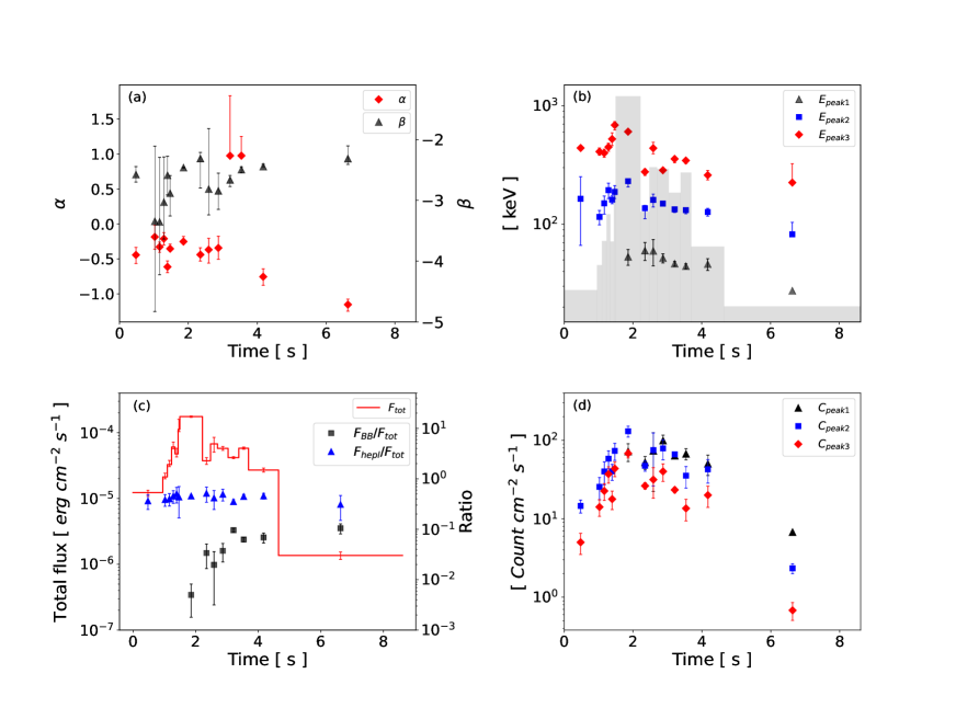
Figure 4: The temporal evolution of the model parameters characterising the spectral shape: (a) $\alpha$ (red diamond) and $\beta$ (black triangle); (b) spectral peaks, $E_{peak1}$ (black triangle), $E_{peak2}$ (blue square) and $E_{peak3}$ (red diamond) are shown. In plot (b), the light curve is shown in shaded grey in the background for reference. (c) The temporal evolution of the total energy flux of the burst, $F_{tot}$, along with the ratios of the thermal energy flux ($F_{BB}$) and energy flux in the extended power law region of the spectrum, $F_{hepl}$ to the total energy flux are shown in red step line, black square and blue triangle respectively. Furthermore, in (d) the temporal evolution of the photon counts fluxes at the spectral peaks, $C_{peak1}$, $C_{peak2}$ and $C_{peak3}$ are shown in black triangle, blue square and red diamond respectively. Note that since the BB component was not constrained until $1.49$ s, the corresponding parameters are absent in the aforementioned plots.

4 Physical Modelling

4.1 Inconsistencies with synchrotron and sub-photospheric dissipation models

The non-thermal nature of the GRB spectrum is commonly attributed to different radiation mechanisms, such as synchrotron radiation (Rees & Meszaros, 1994a; Tavani, 1996; Papathanassiou & Meszaros, 1996; Beniamini et al., 2018) or emissions originating from the photosphere, wherein subphotospheric dissipation (Rees & Mészáros, 2005; Pe’er & Waxman, 2004, 2005; Beloborodov, 2010) leads to spectral shapes that significantly deviate from a simple blackbody or that from a non-dissipative photosphere (Pe’er, 2008; Beloborodov, 2011; Lundman et al., 2013). Nevertheless, our study indicates that the emission detected from GRB131014A is unlikely to originate from these aforementioned two processes. Below we discuss the reasons supporting this inference.

The distinguishing aspect of the GRB131014A spectrum lies in the occurrence of multiple breakpoints. As evident in Figure 3, the $\nu F_{\nu}$ plot exhibits several peaks denoted as $E_{peak1}$, $E_{peak2}$, and $E_{peak3}$. Notably, there is an additional break marked by the extended high-energy power law. The spectrum beyond this break deviates significantly from the spectral turnover observed after $E_{peak3}$. Furthermore, within the burst’s bright region, it’s observed that the low-energy power law index predominantly maintains values $\geq-0.5$ and, in certain instances, approaches $+1$.

When considering a synchrotron spectrum, if $E_{peak3}$ is associated to either $\nu_{m}$ or $\nu_{c}$ for fast or slow cooling synchrotron emission, respectively, (Sari et al., 1998) then the additional breakpoint emerging from the extended power law cannot be explained in a typical synchrotron spectrum, especially at higher energies. Furthermore, the steep $\alpha$ values, approaching nearly $+1$, if associated with the spectral region below synchrotron absorption frequency, would necessitate an exceptionally high bulk Lorentz factor ($\Gamma\geq 1000$) of the outflow and also requires huge magnetic fields in order to position the absorption peak within the X-ray frequency range (Granot et al., 2000; Lloyd & Petrosian, 2000). Among the diverse modified versions of synchrotron emission models, Burgess et al. (Burgess et al., 2019) proposed a synchrotron model that incorporates time-dependent cooling of accelerated electrons. This model was demonstrated to successfully fit approximately $95\%$ of time-resolved peak GRB spectra, encompassing both soft and hard $\alpha$, surpassing even the $\alpha=-0.67$ threshold known as the ”line of death” for synchrotron emission (Preece et al., 1998). However, within these notably successful fits illustrated in Figure 4 of Burgess et al. (Burgess et al., 2019), the likelihood of achieving a successful fit to a spectrum characterised by $\alpha=+1$ is exceedingly low.

Alternatively, another model to explain the GRB spectrum is the sub-photospheric dissipation emission model. The presence of multiple breakpoints within the spectrum negates the plausibility of continuous dissipation occurring from far below up to the photosphere (Beloborodov, 2010; Giannios, 2012; Beloborodov, 2013). When exploring localised sub-photospheric dissipation models, such as those discussed in (Pe’er & Waxman, 2004, 2005), the studies by Ahlgren et al. (Ahlgren et al., 2015, 2019, 2022) wherein the model is directly tested with data, has revealed that for sub-photospheric dissipation occurring at moderate optical depths, the spectrum at high energies beyond the highest peak tends to exhibit a very steep profile (refer to the $\nu F_{\nu}$ plots depicted in Figure 1 in Ahlgren et al. (Ahlgren et al., 2019)). However, in the case of GRB131014A, the high-energy spectrum doesn’t showcase a cutoff; instead, it displays an extended power law characterised by a slope of approximately $-2.4$, persisting until energies around $1\,GeV$.

Therefore, upon evaluating the observational spectral characteristics of the burst in contrast to the expected behaviours of synchrotron and sub-photospheric dissipation models, the prevailing physical scenario appears to be consistent with optically thin inverse Compton scattering of the seed thermal photons originating from the photosphere.

4.2 Proposed Physical Scenario: Optically thin Inverse Compton

In the baryonic fireball model (Goodman, 1986; Paczynski, 1986) scenario, the prompt gamma ray emission is composed of the thermal emission that gets decoupled from the jet photosphere while the non-thermal emission is produced in the optically thin region above the photosphere. The kinetic energy of the outflow may get dissipated via processes like internal shock mechanism (Rees & Meszaros, 1994b; Sari et al., 1996; Kobayashi et al., 1997; Daigne & Mochkovitch, 1998), collisional dissipation (Beloborodov, 2010), etc., in the optically thin region resulting in shocks wherein the electrons get accelerated to relativistic speeds. In the absence of strong magnetic fields, the electrons lose energy via upscattering of the soft thermal photons advected from the photosphere leading to the formation of a non-thermal spectrum. This scattering processes is referred to as the optically thin inverse Compton scattering (ICS). In modeling the spectrum of the burst GRB 131014A, we examine inverse Compton scattering involving only single order of scatterings within an optically thin medium (please refer section 5.4 more details). This results in an ICS spectrum which conforms to the electron distribution’s profile (refer to Appendix B). The post-shock electron distribution (Ellison & Double, 2004; Spitkovsky, 2008; Baring, 2011; Summerlin & Baring, 2012; Burgess et al., 2014) in the outflow is considered to be encompassed of electrons in a thermal pool as well as those accelerated into a power-law tail, as given by

$$n_{e}(\gamma_{e})=n_{0}\left[\left(\frac{\gamma_{e}}{\gamma_{th}}\right)^{2}e^{-\gamma_{e}/\gamma_{th}}+\epsilon\left(\frac{\gamma_{e}}{\gamma_{th}}\right)^{-\delta}\Theta\left(\frac{\gamma_{e}}{\gamma_{min}}\right)\right]$$ (1)

where, $n_{e}$ is the number of electrons with Lorentz factor, $\gamma_{e}$; $n_{0}$ is the normalisation, $\gamma_{th}$ is the thermal electron Lorentz factor, $\gamma_{min}$ is the minimum electron Lorentz factor for the power law tail and is considered to be $\kappa\gamma_{th}$, $\epsilon$ is the normalization of the power law, and $\delta$ is the electron spectral index. $\Theta$(x) is the step function with $\Theta$(x) = 0 for x $<$ 1 and $\Theta$(x) = 1 for x $\geq$ 1. Several studies of Monte Carlo simulations of particle acceleration at relativistic shocks have indicated that the non-thermal population is directly derived from the thermal population (Spitkovsky, 2008; Baring & Braby, 2004) such that $\epsilon/\kappa^{2+\delta}\leq 0.1$. Furthermore, following the approach in Burgess et al. (2014), in order to have a minimised discontinuous transition between the thermal and non-thermal parts of the electron distribution, the value of $\epsilon$ is set to a small numerical value of $\kappa^{2}e^{-\kappa}$. Using the above constraint deduced from the simulations, the $\kappa$ can have values $\geq 1.5$. In this work, we use $\kappa=2$ which is found to be consistent with the values inferred for $\gamma_{min}$ and $\gamma_{th}$ from equation (13). The equation (1) is, thereby, simplified in terms of only three independent variables: $n_{0}$, $\gamma_{min}$ and $\delta$ as follows

$$n_{e}(\gamma_{e})=n_{0}\left[\left(\frac{2\gamma_{e}}{\gamma_{min}}\right)^{2}e^{\frac{-2\gamma_{e}}{\gamma_{min}}}+\ 4e^{-2}\left(\frac{2\gamma_{e}}{\gamma_{min}}\right)^{-\delta}\Theta\left(\frac{\gamma_{e}}{\gamma_{min}}\right)\right]$$ (2)

Note that due to single-order scattering, the thermal pool of electrons is anticipated to generate a corresponding spectral peak, while the extended power law distribution of the electrons is expected to produce a power law within the observed spectrum at higher energies.

The degree of Comptonisation in a medium is defined by the Compton $y$ parameter (Rybicki & Lightman, 1986a) which is given by the product of the average number of scatterings and the average fractional photon energy change per scattering. If $y$ $\gtrsim$ 1, the incident photon energy and the overall spectrum will undergo significant changes. If $y$ $\ll$ 1, the incident photon energy and spectrum minimal change is expected. Neglecting the down scattering of photons, the up-scattered photon energy ($x_{f}$) can be expressed in terms of the Compton $y$ parameter and the photon energy ($x_{0}$) before scattering as (Ghisellini, 2013)

$$x_{f}=x_{0}e^{y}$$ (3)

The mean amplification $A$ of the photon energy at each scattering is given by,

$$A=\frac{x_{f}}{x_{0}}$$ (4)

The equations (3) and (4), yields the Compton $y$ parameter in terms of the mean amplification factor as follows,

$$y=ln(A)$$ (5)

Furthermore, in the optically thin relativistic medium, the average number of scatterings is equivalent to the optical depth at the site, $\tau$ and using the definition of Compton $y$ parameter (Rybicki & Lightman, 1986b; Ghisellini, 2013), the optical depth at the dissipation site can be estimated as

$$\tau=\frac{y}{A-1}$$ (6)

Knowing the optical depth $\tau$ at the dissipation site further allows to estimate the dissipation radius as follows

$$R_{d}=\frac{R_{ph}}{\tau}$$ (7)

where $R_{ph}$ is the photospheric radius.

The average energy of the up-scattered photon can be expressed in terms of the average electron’s Lorentz factor in thermal part of the electron distribution, $\langle\gamma_{e}\rangle$, (Longair, 2011; Rybicki & Lightman, 1986a), as follows

$$x_{f}=\left(\frac{4}{3}\langle\gamma_{e,th}^{2}\rangle\langle\beta_{e,th}^{2}\rangle\right)x_{0}$$ (8)

where, $\langle\beta_{e,th}^{2}\rangle$ = $(1-\frac{1}{\langle\gamma_{e,th}^{2}\rangle})$ = $\frac{\langle v_{e}^{2}\rangle}{c^{2}}$, $\langle v_{e}^{2}\rangle$ is the average of the square of electron’s velocity in the thermal part of the electron distribution and $c$ is the velocity of light. Using equations (4) and (8), the average electron Lorentz factor can be expressed as follows:

$$\langle\gamma_{e,th}^{2}\rangle=\frac{3}{4}A+1$$ (9)

At asymptotic higher energies, the ICS spectrum generated by the power-law distribution of electrons is approximately described as follows (Aharonian & Atoyan, 1981)

$$C_{asym}\propto x_{f}^{-(\delta+1)}$$ (10)

where $C_{asym}$ is the counts flux of ICS photons at the asymptotic higher energies.

4.2.1 Estimating Physical Parameters from Observables

In the proposed physical scenario, we recognize ($E_{\text{peak2}}$ + $E_{\text{peak2}}$)/2 as the peak energy resulting from the first-order inverse Compton scattering of the blackbody (BB) component ($E_{peak1}$) by electrons in the thermal portion of the electron distribution. The amplification factor $A$, is thereby determined as follows

$$A=\frac{E_{peak2}+E_{peak3}}{2E_{peak1}}$$ (11)

The higher energy spectral peak part of the spectrum is produced by the inverse Compton scattering off the electrons with Lorentz factors ranging between $\gamma_{e}$ = 1 to $\gamma_{min}$. Thus, the average electron Lorentz factor of the thermal part of the electron distribution, $\langle\gamma_{e,th}^{2}\rangle$ applicable in equation (9) is estimated as follows

$$\langle\gamma_{e,th}^{2}\rangle\ =\frac{\int_{1}^{\gamma_{min}}\gamma_{e}^{2}n_{e}(\gamma_{e})\,d\gamma_{e}}{\int_{1}^{\gamma_{min}}n_{e}(\gamma_{e})\,d\gamma_{e}}$$ (12)

Using equation (2)

$$\langle\gamma_{e,th}^{2}\rangle=\left[\frac{-5}{2e^{2}}\gamma_{min}^{2}+\left(1+\gamma_{min}+\frac{1}{2}\gamma_{min}^{2}\right)\,e^{\frac{-2}{\gamma_{min}}}\right]^{-1}\\ \times\left[\frac{-21}{2e^{2}}\gamma_{min}^{4}+\left(1+2\gamma_{min}+3\gamma_{min}^{2}+3\gamma_{min}^{3}+\frac{3}{2}\gamma_{min}^{4}\right)e^{\frac{-2}{\gamma_{min}}}\right]$$ (13)

Using equations (9), (11) and (13), $\gamma_{min}$ is estimated using the observed parameters $E_{peak1}$,$E_{peak2}$ and $E_{peak3}$. Given the expression (10) for the asymptotic high energy part of the ICS spectrum, using the observable of the high energy spectral index, $\beta$ allows to estimate the electron power law index $\delta$ as follows (10)

$$\delta=-\beta-1$$ (14)

The normalisation, $n_{0}$ of the electron distribution can be estimated using the estimate of total number of electron in the shock region, $R_{d}$ which is given as

$$N_{e}=\frac{L}{m_{p}c^{3}\Gamma^{2}}R_{d}$$ (15)

where $L$ is the total burst luminosity given by $L=4\pi d_{L}^{2}\,YF_{tot}$, $d_{L}$ is the luminosity distance, $1/Y$ is the radiation efficiency and $F_{tot}$ is the observed total flux, $m_{p}$ is the mass of proton and $\Gamma$ is the bulk Lorentz factor.

The total number of electrons in the shock region can also be evaluated by integrating the electron distribution function given by equation (2) for all possible values of its Lorentz factor,

$$N_{e}=\int_{1}^{\infty}n_{e}(\gamma_{e})\,d\gamma_{e}$$ (16)

leading to the following

$$N_{e}=n_{0}\frac{\gamma_{min}}{2}\left[2+\frac{2^{-\delta+3}}{\delta-1}e^{-2}\right]$$ (17)

Solving equations (15) and (17), the expression of $n_{0}$ can be obtained in terms of $\gamma_{min}$, $\delta$, $L$ and the outflow parameters ($R_{d}$ and $\Gamma$, see section 4.3) which in turn are estimated using the spectral observables.

The number of electrons in the power law tail of the electron distribution is given as follows

$$N_{e,pow}=n_{0}\frac{\gamma_{min}}{2}\frac{2^{-\delta+3}}{\delta-1}e^{-2}$$ (18)

4.3 Outflow parameters

In the physical model interpretation of the burst spectrum, the blackbody component identified in the best fit spectral model is considered as the thermal emission advected from the photosphere of the jet. Associating the observed BB component to the photospheric emission allows to estimate the jet outflow parameters such as the Lorentz factor ($\Gamma$) at the photosphere; the nozzle radius ($R_{0}$): the radius from where the jet starts to expand freely; the saturation radius ($R_{s}$): the radius where the internal energy density of the jet becomes equal to the kinetic energy of the jet; and the photospheric radius ($R_{ph}$): the radius at which the photons get decoupled from the plasma, using the methodology given in (Pe’er et al., 2007; Iyyani et al., 2013, 2016). For an assumed redshift $z=2.12$, an average value for the GRBs with LAT data and a radiative efficiency $1/Y=0.65$ (Racusin et al., 2011), the average values of the outflow parameters are as follows: $\Gamma=400\pm 6$, $R_{0}$ = $(2.4\pm 1.1)\times 10^{8}$ cm, $R_{s}$ = $(8.4\pm 0.8)\times 10^{10}$ cm and $R_{ph}$ = $(1.8\pm 0.3)\times 10^{13}$ cm.

The temporal evolution of the outflow parameters is shown in Figure 5, except for the first six bins up to 1.49 s, as the BB component is not constrained during this period. Among the radial parameters, the nozzle radius, $R_{0}$ is found to increase with time from nearly close to the central engine of around several $10^{6}\,\rm cm$ to a peak value of around $10^{9}\,\rm cm$ and later remains nearly steady with time (Figure 5a). This temporal behaviour is consistent with that observed in previous studies (Iyyani et al., 2013, 2015, 2016). A corresponding similar trend is observed in $R_{s}$ as well. The photospheric radius is found to be nearly steady with only mild variations around $10^{13}$ cm (Figure 5a).

The Lorentz factor ($\Gamma$) of the outflow shows predominantly a monotonous decrease from an initial value of nearly $700$ to around $200$ across the total burst duration as evident in Figure 5b. It is noteworthy that despite multiple emission pulses during the total burst duration, on average, the Lorentz factor of the outflow keeps decreasing with time.

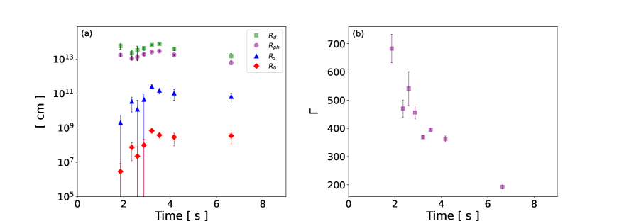
Figure 5: The evolution of the jet outflow parameters including (a) nozzle radius, $R_{0}$ (red diamond); saturation radius, $R_{s}$ (blue triangle); photopsheric radius, $R_{ph}$ (magenta circle), dissipation radius, $R_{d}$ (green square) and (b) the bulk Lorentz factor, $\Gamma$ with time are shown.

4.4 Inverse Compton Characteristics

The estimates of the physical parameters that characterize the optically thin inverse Compton scattering using the equations mentioned in subsection 4.2 are discussed here. The average estimates for the physical parameters are mentioned along with their temporal behaviours.

The mean amplification factor, $A$ and the Compton $y$ parameter are found to be $5.06\pm 0.20$ and $1.60\pm 0.08$ respectively. The value of $y\gtrsim 1$ suggests a substantial spectral change due to the inverse Compton scattering process. The temporal variation of these parameters is shown in Figure 6a. The optical depth ($\tau$) at which the dissipation shocks are generated is found to be $0.41\pm 0.05$ which indicates that the dissipation is taking place in the optically thin region of the jet (Figure 6b). This further gives the estimate of the dissipation radius which is found to lie closely above the photosphere, within the range of $10^{14}$ cm as shown in Figure 5a. We note that no significant trend is observed in the temporal evolution of these parameters during the burst duration.

The estimates of the parameters characterising the electron distribution presented in section 4.2 are discussed below. The $\gamma_{min}$, $\langle\gamma_{e,th}\rangle$, $\delta$ and $n_{0}$ are found to be $3\pm 0.07$, $2.17\pm 0.07$, $1.54\pm 0.05$ and $(4.0\pm 1.0)\times 10^{54}$ respectively. The temporal evolution of these parameters are shown in Figure 7a and 7b respectively. The total number of electrons, $N_{e}$ is found to be around $1.5\times 10^{55}$, while the ratio of the number of electrons in the power law tail of the electron distribution to the total number of electrons, $N_{e,pow}$/$N_{e}$ is around $20\%$ which is relatively higher than what is reported in particle in cell (PIC) simulation studies (Spitkovsky, 2008). The temporal variation of the parameters is shown in 7c. The total number of electrons is found to increase by an order of magnitude to around a several $10^{55}$ during the initial pulses of the burst, however, decreases to around several $10^{53}$ after $3.5$s (Figure 7c).

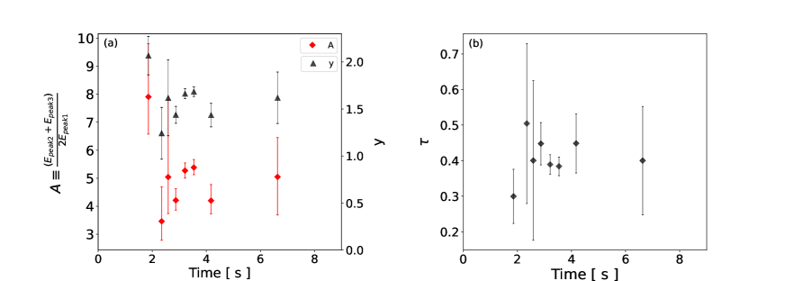
Figure 6: The temporal evolution of the microphysical parameters of the inverse Compton scattering such as (a) amplification parameter, $A$ (red diamond), Compton $y$ parameter (black triangle), and (b) optical depth $\tau$ (black diamond) at the dissipation site are shown.

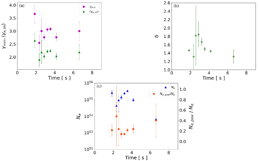
Figure 7: The temporal evolution of the parameters of the electron distribution at the dissipation site: (a) minimum electron Lorentz factor $\gamma_{min}$ (magenta circles), average electron Lorentz factor of the thermal part of the electron distribution, $\langle\gamma_{e,th}\rangle$ (green triangles), (b) power law index, $\delta$ (green diamond) and (c) total number of electrons, $N_{e}$ (blue triangle) along with the ratio of electrons in the power law with respect to the total number of electrons ($N_{e,pow}/N_{e}$, red square) are shown.

5 Discussion

5.1 Multiple breaks in GRB spectrum

A primary observational finding in the spectral analysis of Fermi-detected GRBs indicates that among the brightest instances, the time-resolved GRB spectra significantly differ from a singular Band function (Ackermann et al., 2013). These variations involve multiple additional components, such as a blackbody function at lower energies (Guiriec et al., 2011; Axelsson et al., 2012; Burgess et al., 2014; Iyyani et al., 2015), an extra power law extending to higher energies (Abdo et al., 2009; Ryde et al., 2010, 2011; Iyyani et al., 2015; Sharma et al., 2019) or a power law with an exponential cutoff (Ackermann et al., 2011). Some cases even show multiplicative components, like an exponential cutoff at higher energies (Ackermann et al., 2011; Vianello et al., 2018; Sharma et al., 2019).

GRB131014A aligns with these findings, displaying a spectrum that doesn’t conform to a simple, conventional Band function alone. The spectrum of GRB131014A exhibits distinctive features, including a thermal component at lower energies, as well as two spectral breaks identified at energies $E_{peak2}$ and $E_{peak3}$. Moreover, the trend of the turnover of the spectrum beyond $E_{peak3}$ is obscured by the extension of the high-energy power law, resulting in an additional spectral break at higher energies, indicating the onset of the extended power law. This unique spectral shape is reported here for the first time. Furthermore, we note that the ratio between the highest spectral peak ($E_{peak3}$) and the lowest spectral peak ($E_{peak1}$) is approximately about an order of magnitude. The complexity of this spectral shape poses challenges for modeling with simple empirical functions such as the Band function, cutoff power law, or smoothly broken power law. Consequently, multiple empirical functions, including two Band functions and a blackbody, were employed in an additive fashion in order to capture its features.

Furthermore, we note that GRB131014A was previously examined by Guiriec et al. (Guiriec et al., 2015), who focused solely on GBM data, excluding LLE and LAT emissions. Consequently, they may have overlooked the high-energy spectral break and extended power-law identified in our study.

5.2 Non-detection of BB in initial bins

Guiriec et al. (Guiriec et al., 2015) observed a robust thermal component in the spectrum of GRB131014A while conducting a detailed time-resolved spectral analysis with bin widths ranging from 2 ms to 94 ms (Guiriec et al., 2010). This analysis revealed initially hard low-energy spectral slopes ranging from $0$ to $+1$ during the burst’s early stages. In contrast, our study employs Bayesian Block binning for time-resolved analysis, resulting in broader time intervals and relatively softer $\alpha$ values ($\geq-0.5$) for the considered model. Acuner et al. (Acuner et al., 2019) demonstrated that synthetic spectra generated by convolving the theoretical model of non-dissipative photospheric emission ($\sim$ thermal component) with Fermi GBM’s response yielded $\alpha$ values ranging between $-0.4$ and $0.0$ when modeled using empirical functions like the Band function. Hence, our observation of $\alpha\geq-0.5$ strongly suggests a notable thermal contribution at lower energies within the burst spectrum, aligning with the findings of Guiriec et al. (Guiriec et al., 2015). Additionally, we observe that the thermal peak values reported by Guiriec et al. (Guiriec et al., 2015) during the initial time bins until 1.49 s range from approximately 100 keV to 200 keV (refer to Figure 2c in (Guiriec et al., 2015)), which corresponds well with the $E_{peak2}$ values identified in our analysis (refer to Figure 4b). Thus, it is worth noting that the thermal component of the best-fit model discussed in this current study differs from that referenced in Guiriec et al.’s work.

In our physical model interpretation, we have considered the GRB131014A to possess a baryon-dominated jet, which is typically expected to produce prominent thermal detections, in contrast to Poynting flux-dominated outflows, where the photospheric emission is highly suppressed (Zhang & Pe’er, 2009). However, our analysis fails to constrain the thermal component in the initial bins until 1.49 s. On extrapolating the observed trend of the ratio of thermal flux to the observed total flux (Figure 4c) in to the earlier time bins indicates that the expected thermal flux is much less than $1\%$. In addition, the trend of the thermal peak ($E_{peak1}$) on extrapolating to times before 1.49s also indicates values less than 40 keV which corresponds to $kT\ll 10\,\rm keV$. As the thermal component approaches lower fluxes as well as the edge of the observation window of the Fermi GBM makes it technically and statistically challenging to determine the component in the early time bins.

5.3 Microphysics of shock and electron cooling

In the optically thin region of the outflow where the kinetic energy of the outflow is dissipated via some dissipation mechanism to form diffusive shocks in the plasma cause the acceleration of certain fraction of electrons from the thermal pool to very high energies, producing a high energy power law tail. The values of the power law index, $\delta$, of the electron distribution 2 reveals some crucial characteristics of the shock and the background medium. For the diffusive acceleration at the parallel, ultra-relativistic shocks, the accepted value of $\delta$ is 2.2 (Kirk & Schneider, 1987; Kirk et al., 2000). However, if the background medium has pressure anisotropy, the $\delta$ may decrease below 2 in the scenario where the influence of pressure anisotropy on shock compression is significant (Double et al., 2004; Baring, 2006). The estimated values of $\delta$ for the GRB131014A, remain below 2 throughout the burst duration as shown in the Figure 7. This indicates that the plasma of GRB131014A where shocks are produced, has significant pressure anisotropy. The average value of $\gamma_{e}$ is estimated by considering the total electron distribution including both the thermal and non-thermal part of distribution 2. Although Fermi LAT can detect photons of energy up to 300 GeV, the maximum observed photon energy for the GRB131014A is 1.8 GeV. This implies that many photons with energies exceeding 1.8 GeV might not have been produced. This observed limit on the maximum energy of photons provides constraints on the maximum electron Lorentz factor ($\gamma_{max}$), which corresponds to nearly an order of $10^{4}$ ($\gamma_{max}$ $m_{e}c^{2}$ $\approx$ few GeV). Using this upper limit, the average value of $\gamma_{e}$ is estimated to be $\langle\gamma_{e}\rangle$ $\approx$ $10^{3}$. This allows us to further estimate the total energy of the electrons in the lab frame which is $E_{el}=\Gamma N_{e}\,\langle\gamma_{e}\rangle\,m_{e}c^{2}=5\times 10^{54}$ erg, where $\Gamma=400$ and $N_{e}=1.5\times 10^{55}$ for the time integrated spectrum. Thus, around $20\%$ of the total burst energy is allocated to the electrons in the shocked region.

For the ICS to be the dominant emission process over the synchrotron radiation, requires that the ratio $u_{ph}/u_{B}$ be higher than unity (Rybicki & Lightman, 1986a) where $u_{B}$ is the magnetic energy density and $u_{ph}$ is the radiation energy density due to the thermal emission at the dissipation site ($R_{d}\sim 10^{14}\,\rm cm$). The ratio can be rewritten as

$$\frac{u_{ph}}{u_{B}}=\frac{E_{ph}}{E_{B}}\equiv\frac{E_{BB}}{E_{B}}>1$$ (19)

where $E_{B}$ is the total magnetic energy and $E_{BB}$ is the total energy of the BB component of the observed spectrum for the entire burst duration which is estimated to be around $4\times 10^{53}$ erg. Substituting this value into equation 19 suggests that $E_{B}$ is less than $4\times 10^{53}$ erg, indicating that the total magnetic energy comprises less than $1\%$ of the total burst energy. Additionally, it suggests that the magnetic field intensity at the dissipation site, denoted by $B$, is less than approximately $10^{6}$ Gauss.

Furthermore, the accelerated electrons in the shock region of the outflow cool on time-scales in the co-moving frame given by $t^{\prime}_{cool}\simeq 3m_{e}c/4\gamma_{e}\sigma_{T}u_{ph}$, where $\sigma_{T}$ is the Thomson cross-section. The thermal energy density at the dissipation radius, $R_{d}\sim 10^{14}\,\rm cm$ is estimated to be $u_{ph}=2.4\times 10^{13}$ erg/$cm^{3}$. Thus, the Compton cooling time-scale for the electrons is found to be around $1.3\times 10^{-9}$ s which is much lesser than the dynamical time-scale, $t^{\prime}_{dyn}$ = $R_{d}$/$\Gamma$c = 6.75 s, indicating that the Compton cooling is much efficient during the prompt emission of the burst.

5.4 Insignificance of higher order ICS

Based on the calculations conducted in the preceding sections, we find that the kinetic energy dissipation of the jet occurs within the optically thin region spanning from $10^{13}$ to $10^{14}$ cm. Although the outflow progresses to a region where the probability of photon-electron scattering diminishes, there is still significant opacity due to photon-photon interactions. In the currently observed first order scattered part of the spectrum, it is observed that $8.6\times 10^{54}$ photons have energies exceeding 500 keV in the co-moving frame, assuming a burst Lorentz factor $\Gamma=400$. Taking this as a conservative estimate for the number of photons produced above 500 keV in the co-moving frame, we deduce that the compactness parameter, $l$, reaches unity at distances greater than $10^{14}$ cm. Consequently, throughout the duration of the burst, the dissipation site consistently falls within the region where $l>1$. This implies that combining photons that meet the pair production threshold ($>2m_{e}c^{2}$) can lead to pair production at the dissipation site.

The presence of a high-energy tail extending to several GeVs suggests that, subsequent to pair production, the optical depth at the dissipation site should remain at or below 1. Applying this constraint and setting $\tau_{\gamma,e}=1$ we calculate that the number of generated pairs should be approximately $8.5\times 10^{54}$. Let $N$ represent the actual number of photons above 500 keV. Only a fraction of $N$ converts into pairs, while the remaining contributes to the observed spectrum. Based on these constraints, we estimate that approximately less than or equal to $50\%$ of the photons with energies exceeding 500 keV have undergone pair production. As the total energy in electrons remains constant, the increase in leptonic particles post pair production reduces the $\gamma_{e}$ from nearly 1000 (as mentioned in section 5.3) to 370 post first order scattering.

In the overall electron distribution, the thermal component predominantly has values with $\gamma_{e}<3$. Therefore, the average $\gamma_{e}$ is mainly influenced by the values of $\gamma_{e}$ within the power-law distribution. Consequently, the observed decrease in the average, $\gamma_{e}$, can result from a steepening of the electron power-law index as well as when the minimum, $\gamma_{min}$, of the power-law shift towards the thermal part of the electron distribution. In both cases, the lower values of $\gamma_{e}$ carry more weight, reducing the average, $\gamma_{e}$.

Reduced values of $\gamma_{min}$ can, in turn, decrease the $\gamma_{th}$ of the electron distribution. As a result, the average $\gamma_{e,th}$ will decrease, causing the second-order Compton scattered peak to likely occur at energies lower and at reduced energy fluxes than anticipated. Thus, it is likely that the second-order scattered peak will only minimally impact the total observed flux of the first-order scattering.

In the proposed scenario of potential pair production occurring at the dissipation site, we anticipate that higher-order scatterings will be less significant within the current interpretation of the physical model presented.

6 Summary & Conclusion

In this study, we investigate in detail the radiation mechanism of the prompt emission of GRB131014A. The detailed time resolved spectral analysis of the GRB revealed that the spectrum is more complex than the typical Band function. The spectrum has an unconventional shape with three spectral peaks and an extended high energy power law tail, best fitted by 2Bands + blackbody model with high statistical significance. The overall shape of the spectrum is characterized by five parameters namely lower energy power law index $\alpha$, higher energy power law index $\beta$ and the three spectral peaks $E_{peak1}$, $E_{peak2}$ and $E_{peak3}$. Such a complex spectral shape is reported for the first time.

The persistently hard $\alpha$ values, surpassing $-0.5$ and occasionally reaching up to $+1$, defy an explanation through synchrotron radiation. Moreover, the presence of an extended power law extending to several GeV, rather than exhibiting a cutoff beyond the highest spectral peak, contradicts localized sub-photospheric dissipation models. Therefore, the overall spectral shape, featuring an extended power law, is more likely consistent with first-order inverse Compton scattering. In this scenario, thermal photons advected from the photosphere undergo upscattering by electrons accelerated in the shock region within the optically thin outflow. The resulting spectrum reflects the shape of the post-shock electron distribution, which comprises both a thermal component and a power-law component.

Within this physical framework, we characterize the properties of inverse Compton scattering, including the amplification factor and Compton $y$ parameter, and determine electron distribution parameters, such as the electron power-law index, which is around $1.5$. Despite multiple emission episodes occurring throughout the burst duration, the Lorentz factor of the outflow steadily decreases over time. Concurrently, the nozzle radius of the jet initially expands from nearly $10^{6}$ cm to approximately $10^{9}$ cm before becoming steady. This temporal behavior of the outflow aligns with the observations of single-pulsed emission GRBs. The shock region is estimated to lie just above the photosphere at an optical depth of $0.4$. Furthermore, our analysis indicates that approximately $20\%$ of the total burst energy goes into electrons, while less than $1\%$ goes to magnetic fields. Moreover, given that the dissipation site is well within the photon compactness region, we suggest that a portion of the upscattered photons in the first-order scattering, exceeding 500 keV in the co-moving frame, undergo pair production, ensuring that the resulting optical depth remains unity. This pair production is anticipated to lead to a decrease in the average electron Lorentz factor across both the thermal and power-law components of the electron distribution. Consequently, higher-order scatterings are suppressed, having a minimal impact on the observed first-order scattered inverse Compton spectrum.

In conclusion, this study offers a thorough identification and detailed modeling of optically thin inverse Compton scattering in the prompt emission of GRB 131014A.

Appendix A Fit parameters of the best fit model

In Table 1, the fit values for the eight free parameters of the best-fit model of ’2 Bands’ up to 1.49 s, and the ten free parameters of the best-fit model of ’2 Bands + Blackbody’ above 1.49 s, are listed. Additionally, the $\Delta$ AIC ($\rm AIC_{\rm model}-\rm AIC_{\rm best\,model}$) values for the various models relative to the best-fit model in each time interval are also provided.

Appendix B Comparison with Simulated Inverse Compton spectrum

Using the electron distribution characteristics obtained in section 4.4 for one of the brighter time intervals, i.e [3.04s - 3.38s] (Figure 8) and the blackbody function of temperature 12 keV as the seed photon distribution, a first order inverse Compton scattering spectrum is simulated using the Naima package (Zabalza, 2015). The obtained simulated spectrum is shown in Figure 9 is found to closely resemble the observed spectrum of the same interval shown on the left in the Figure 9. This preliminary analysis provides encouraging results supporting the physical scenario that the observed spectrum is a result of first-order optically thin inverse Compton scattering of photospheric emission. In a subsequent future work, we aim to directly model the GRB data with the ICS model using the Naima package.

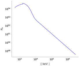
Figure 8: Post-shock electron distribution with $\delta$=1.7, $\gamma_{min}$=3.06, $n_{0}$=6.98$\times$$10^{54}$ is shown.

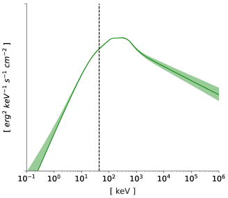
(a) Observed spectrum

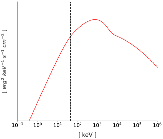
(b) Simulated spectrum

Figure 9: Comparison between the observed and simulated spectra. (a) Observed spectrum best fitted by 2Bands + Blackbody model is shown in green solid line. (b) Simulated spectrum of first order inverse Compton scattering is shown. The black dashed vertical lines represent blackbody temperature at 12 keV.

Time-resolved analysis results

Time intervals (s)

Blackbody

Band1

Band2

$\Delta$AIC = AICmodel - AIC${}_{best\,model}$

K (cm-2keV-3s-1)

kT (keV)

K1 (cm-2keV-1s-1)

$\alpha_{1}$

$\beta_{1}$

Epeak1 (keV)

K2 (cm-2keV-1s-1)

$\alpha_{2}$

$\beta_{2}$

Epeak2 (keV)

$Band$

$Band+BB$

$Band+CPL$

$2Band$

$Band+CPL+BB$

0.00 - 0.95

None

None

0.35${}^{+0.15}_{-0.17}$

0.80${}^{+0.62}_{-0.67}$

-2.55${}^{+0.16}_{-0.15}$

164${}^{+23}_{-21}$

0.09${}^{+0.02}_{-0.02}$

-0.44${}^{+0.13}_{-0.13}$

-4.99${}^{+0.04}_{-0.01}$

440${}^{+51}_{-61}$

4

1

0

0

None

0.95 - 1.09

None

None

1.04${}^{+0.54}_{-0.51}$

0.80${}^{+0.64}_{-0.62}$

-3.09${}^{+0.91}_{-1.15}$

115${}^{+16}_{-17}$

0.26${}^{+0.04}_{-0.04}$

-0.24${}^{+0.20}_{-0.20}$

-4.99${}^{+0.19}_{-0.03}$

410${}^{+30}_{-29}$

4

3

2

0

None

1.09 - 1.23

None

None

1.11${}^{+0.89}_{-0.65}$

1.36${}^{+0.91}_{-0.73}$

-3.17${}^{+0.89}_{-0.99}$

150${}^{+23}_{-29}$

0.43${}^{+0.07}_{-0.07}$

-0.35${}^{+0.10}_{-0.08}$

-4.96${}^{+0.66}_{-0.15}$

399${}^{+32}_{-31}$

4

4

2

0

None

1.23 - 1.34

None

None

0.79${}^{+0.70}_{-0.65}$

3.01${}^{+0.001}_{-0.002}$

-3.24${}^{+1.00}_{-1.14}$

194${}^{+30}_{-30}$

0.64${}^{+0.09}_{-0.08}$

-0.20${}^{+0.09}_{-0.09}$

-3.45${}^{+0.48}_{-0.46}$

449${}^{+36}_{-37}$

3

2

4

0

None

1.34 - 1.44

None

None

3.44${}^{+1.02}_{-1.16}$

3.00${}^{+0.005}_{-0.003}$

-2.55${}^{+0.35}_{-0.25}$

161${}^{+12}_{-11}$

0.31${}^{+0.05}_{-0.05}$

-0.60${}^{+0.09}_{-0.09}$

-2.87${}^{+0.28}_{-0.33}$

525${}^{+64}_{-69}$

1

3

1

0

None

1.44 - 1.49

None

None

2.20${}^{+1.01}_{-1.12}$

2.99${}^{+0.001}_{-0.01}$

-2.85${}^{+0.59}_{-0.74}$

188${}^{+24}_{-25}$

0.56${}^{+0.06}_{-0.05}$

-0.24${}^{+0.08}_{-0.06}$

-4.07${}^{+1.25}_{-0.08}$

687${}^{+47}_{-61}$

1

1

2

0

None

1.49 - 2.22

0.0023${}^{+0.002}_{-0.001}$

13.47${}^{+2.34}_{-2.45}$

2.15${}^{+0.61}_{-0.54}$

1.36${}^{+0.56}_{-0.51}$

-2.44${}^{+0.04}_{-0.04}$

132${}^{+19}_{-22}$

0.80${}^{+0.08}_{-0.08}$

-0.26${}^{+0.06}_{-0.05}$

-3.75${}^{+0.44}_{-0.39}$

606${}^{+23}_{-25}$

137

20

3

0

4

2.22 - 2.47

0.003${}^{+0.002}_{-0.0008}$

15.26${}^{+0.61}_{-4.67}$

8.33${}^{+6.35}_{-3.52}$

2.99${}^{+0.07}_{-0.51}$

-2.29${}^{+0.07}_{-0.10}$

137${}^{+7}_{-26}$

0.52${}^{+0.11}_{-0.10}$

-0.46${}^{+0.12}_{-0.06}$

-4.28${}^{+1.77}_{-0.29}$

277${}^{+15}_{-20}$

6

2

2

3

None

2.47 - 2.70

0.005${}^{+0.004}_{-0.001}$

15.30${}^{+1.38}_{-7.04}$

7.70${}^{+2.22}_{-6.62}$

2.55${}^{+0.07}_{-1.82}$

-2.74${}^{+0.33}_{-0.30}$

161${}^{+14}_{-22}$

0.47${}^{+0.08}_{-0.13}$

-0.40${}^{+0.19}_{-0.13}$

-3.19${}^{+0.44}_{-0.52}$

448${}^{+50}_{-43}$

20

3

4

4

1

2.70 - 3.04

0.004${}^{+0.001}_{-0.001}$

13.20${}^{+1.11}_{-1.12}$

6.82${}^{+1.11}_{-1.25}$

1.90${}^{+0.25}_{-0.25}$

-2.44${}^{+0.04}_{-0.03}$

150${}^{+1}_{-1}$

0.59${}^{+0.05}_{-0.05}$

-0.58${}^{+0.05}_{-0.05}$

-4.99${}^{+0.32}_{-0.04}$

286${}^{+1}_{-1}$

25

9

2

0

1

3.04 - 3.38

0.02${}^{+0.002}_{-0.001}$

11.85${}^{+0.38}_{-0.61}$

25.62${}^{+4.18}_{-3.48}$

3.00${}^{+0.002}_{-0.002}$

-2.67${}^{+0.09}_{-0.08}$

134${}^{+3}_{-8}$

0.19${}^{+0.16}_{-0.04}$

1.97${}^{+0.38}_{-2.09}$

-5.00${}^{+0.002}_{-0.001}$

356${}^{+15}_{-28}$

49

28

26

23

16

3.38 - 3.69

0.02${}^{+0.003}_{-0.002}$

11.27${}^{+0.43}_{-0.68}$

31.58${}^{+6.27}_{-3.44}$

3.00${}^{+0.001}_{-0.001}$

-2.50${}^{+0.06}_{-0.04}$

132${}^{+2}_{-9}$

0.23${}^{+0.16}_{-0.01}$

2.78${}^{+0.13}_{-1.97}$

-4.10${}^{+0.78}_{-0.47}$

345${}^{+14}_{-20}$

42

23

16

13

5

3.69 - 4.65

0.01${}^{+0.004}_{-0.003}$

11.73${}^{+1.17}_{-1.32}$

14.39${}^{+5.06}_{-4.74}$

2.99${}^{+0.005}_{-0.04}$

-2.43${}^{+0.06}_{-0.07}$

127${}^{+9}_{-10}$

0.29${}^{+0.06}_{-0.07}$

-0.74${}^{+0.11}_{-0.10}$

-5.00${}^{+0.003}_{-0.001}$

260${}^{+27}_{-23}$

16

12

6

6

9

4.65 - 8.61

0.003${}^{+0.001}_{-0.0002}$

7.74${}^{+0.10}_{-0.10}$

0.04${}^{+0.005}_{-0.005}$

-1.06${}^{+0.06}_{-0.12}$

-4.99${}^{+0.54}_{-0.06}$

82${}^{+0.5}_{-0.5}$

0.01${}^{+0.001}_{-0.007}$

-1.11${}^{+0.28}_{-0.26}$

-2.29${}^{+0.21}_{-0.14}$

225${}^{+106}_{-10}$

4

4

3

2

1

Time-integrated analysis results

0.00 - 8.61

0.002${}^{+0.0005}_{-0.0005}$

12.39${}^{+0.62}_{-0.62}$

3.41${}^{+0.42}_{-0.41}$

2.99${}^{+0.001}_{-0.001}$

-2.39${}^{+0.03}_{-0.03}$

150.31${}^{+4.28}_{-4.23}$

0.24${}^{+0.01}_{-0.01}$

-0.55${}^{+0.03}_{-0.03}$

-3.33${}^{+0.23}_{-0.22}$

451.34${}^{+11.63}_{-12.29}$

229

79

79

59

30

Table 1: The fit parameters and its errors of the spectral components of the best fit model along with the AIC difference of the different models with respect to the best fit model are listed. In the time-resolved spectral analysis, in the initial 6 time intervals, 2Bands model is considered to be the best fit model while in the remaining 8 time intervals, 2Band + BB is the best fit model. ’None’ indicates that the model could not be fitted to the data. In time-integrated spectral analysis, the best fit model is found to be 2Band + BB.

References

- Abdalla et al. (2019) Abdalla, H., et al. 2019, Nature, 575, 464, doi: 10.1038/s41586-019-1743-9
- Abdo et al. (2009) Abdo, A. A., Ackermann, M., & et al. 2009, ApJL, 706, L138, doi: 10.1088/0004-637X/706/1/L138
- Ackermann et al. (2011) Ackermann, M., Ajello, M., & et al. 2011, ApJ, 729, 114, doi: 10.1088/0004-637X/729/2/114
- Ackermann et al. (2013) —. 2013, ApJS, 209, 11, doi: 10.1088/0067-0049/209/1/11
- Acuner et al. (2019) Acuner, Z., Ryde, F., & Yu, H.-F. 2019, MNRAS, 487, 5508, doi: 10.1093/mnras/stz1356
- Aghanim et al. (2020) Aghanim, N., et al. 2020, Astron. Astrophys., 641, A6, doi: 10.1051/0004-6361/201833910
- Aharonian & Atoyan (1981) Aharonian, F. A., & Atoyan, A. M. 1981, Ap&SS, 79, 321, doi: 10.1007/BF00649428
- Ahlgren et al. (2019) Ahlgren, B., Larsson, J., Ahlberg, E., et al. 2019, MNRAS, 485, 474, doi: 10.1093/mnras/stz110
- Ahlgren et al. (2022) —. 2022, VizieR Online Data Catalog, J/MNRAS/485/474
- Ahlgren et al. (2015) Ahlgren, B., Larsson, J., Nymark, T., Ryde, F., & Pe’er, A. 2015, MNRAS, 454, L31, doi: 10.1093/mnrasl/slv114
- Amaral-Rogers et al. (2013) Amaral-Rogers, A., Evans, P. A., & Page, K. L. 2013, GRB Coordinates Network, 15344, 1
- Asano et al. (2009) Asano, K., Inoue, S., & Mészáros, P. 2009, ApJ, 699, 953, doi: 10.1088/0004-637X/699/2/953
- Axelsson et al. (2012) Axelsson, M., Baldini, L., & et al. 2012, ApJ, 757, L31, doi: 10.1088/2041-8205/757/2/L31
- Band et al. (1993) Band, D., Matteson, J., Ford, L., et al. 1993, ApJ, 413, 281, doi: 10.1086/172995
- Baring (2006) Baring, M. G. 2006, Advances in Space Research, 38, 1281, doi: 10.1016/j.asr.2005.02.004
- Baring (2011) —. 2011, Advances in Space Research, 47, 1427, doi: 10.1016/j.asr.2010.02.016
- Baring & Braby (2004) Baring, M. G., & Braby, M. L. 2004, ApJ, 613, 460, doi: 10.1086/422867
- Beloborodov (2010) Beloborodov, A. M. 2010, MNRAS, 407, 1033, doi: 10.1111/j.1365-2966.2010.16770.x
- Beloborodov (2010) Beloborodov, A. M. 2010, Monthly Notices of the Royal Astronomical Society, 407, 1033, doi: 10.1111/j.1365-2966.2010.16770.x
- Beloborodov (2011) Beloborodov, A. M. 2011, ApJ, 737, 68, doi: 10.1088/0004-637X/737/2/68
- Beloborodov (2013) —. 2013, ApJ, 764, 157, doi: 10.1088/0004-637X/764/2/157
- Beniamini et al. (2018) Beniamini, P., Barniol Duran, R., & Giannios, D. 2018, MNRAS, 476, 1785, doi: 10.1093/mnras/sty340
- Beniamini & Giannios (2017) Beniamini, P., & Giannios, D. 2017, MNRAS, 468, 3202, doi: 10.1093/mnras/stx717
- Burgess et al. (2019) Burgess, J. M., Bégué, D., Greiner, J., et al. 2019, Nature Astronomy, 471, doi: 10.1038/s41550-019-0911-z
- Burgess et al. (2021) Burgess, J. M., Fleischhack, H., Vianello, G., et al. 2021, The Multi-Mission Maximum Likelihood framework (3ML), 2.2.4, Zenodo, doi: 10.5281/zenodo.5646954
- Burgess et al. (2014) Burgess, J. M., Preece, R. D., & et al. 2014, ApJ, 784, 17, doi: 10.1088/0004-637X/784/1/17
- Daigne & Mochkovitch (1998) Daigne, F., & Mochkovitch, R. 1998, Monthly Notices of the Royal Astronomical Society, 296, 275, doi: 10.1046/j.1365-8711.1998.01305.x
- Derishev & Piran (2019) Derishev, E., & Piran, T. 2019, ApJ, 880, L27, doi: 10.3847/2041-8213/ab2d8a
- Dermer et al. (2000) Dermer, C. D., Böttcher, M., & Chiang, J. 2000, ApJ, 537, 255, doi: 10.1086/309017
- Desiante et al. (2013) Desiante, R., Kocevski, D., Vianello, G., et al. 2013, GRB Coordinates Network, 15333, 1
- Double et al. (2004) Double, G. P., Baring, M. G., Jones, F. C., & Ellison, D. C. 2004, ApJ, 600, 485, doi: 10.1086/379702
- Ellison & Double (2004) Ellison, D. C., & Double, G. P. 2004, Astroparticle Physics, 22, 323, doi: 10.1016/j.astropartphys.2004.08.005
- Fitzpatrick & Xiong (2013) Fitzpatrick, G., & Xiong, S. 2013, GRB Coordinates Network, 15332, 1
- Ghisellini (2013) Ghisellini, G. 2013, Radiative Processes in High Energy Astrophysics, Vol. 873, doi: 10.1007/978-3-319-00612-3
- Ghisellini & Celotti (1999) Ghisellini, G., & Celotti, A. 1999, ApJL, 511, L93, doi: 10.1086/311845
- Giannios (2012) Giannios, D. 2012, MNRAS, 422, 3092, doi: 10.1111/j.1365-2966.2012.20825.x
- Golenetskii et al. (2013) Golenetskii, S., Aptekar, R., Frederiks, D., et al. 2013, GRB Coordinates Network, 15338, 1
- Goodman (1986) Goodman, J. 1986, ApJ, 308, L47, doi: 10.1086/184741
- Granot et al. (2000) Granot, J., Piran, T., & Sari, R. 2000, ApJ, 534, L163, doi: 10.1086/312661
- Gruber et al. (2014) Gruber, D., Goldstein, A., & et al. 2014, ApJS, 211, 12, doi: 10.1088/0067-0049/211/1/12
- Guiriec et al. (2011) Guiriec, S., Connaughton, V., & et al. 2011, ApJL, 727, L33, doi: 10.1088/2041-8205/727/2/L33
- Guiriec et al. (2015) Guiriec, S., Mochkovitch, R., Piran, T., et al. 2015, ApJ, 814, 10, doi: 10.1088/0004-637X/814/1/10
- Guiriec et al. (2010) Guiriec, S., Briggs, M. S., Connaugthon, V., et al. 2010, ApJ, 725, 225, doi: 10.1088/0004-637X/725/1/225
- Hurley et al. (2013) Hurley, K., Goldsten, J., Golenetskii, S., et al. 2013, GRB Coordinates Network, 15363, 1
- Iyyani (2018) Iyyani, S. 2018, Journal of Astrophysics and Astronomy, 39, 75, doi: 10.1007/s12036-018-9567-9
- Iyyani et al. (2016) Iyyani, S., Ryde, F., Burgess, J. M., Pe’er, A., & Bégué, D. 2016, MNRAS, 456, 2157, doi: 10.1093/mnras/stv2751
- Iyyani et al. (2013) Iyyani, S., Ryde, F., & et al. 2013, MNRAS, 433, 2739, doi: 10.1093/mnras/stt863
- Iyyani et al. (2015) Iyyani, S., Ryde, F., Ahlgren, B., et al. 2015, MNRAS, 450, 1651, doi: 10.1093/mnras/stv636
- Iyyani et al. (2015) Iyyani, S., Ryde, F., Ahlgren, B., et al. 2015, Monthly Notices of the Royal Astronomical Society, 450, 1651, doi: 10.1093/mnras/stv636
- Kann et al. (2013) Kann, D. A., Kruehler, T., Varela, K., & Greiner, J. 2013, GRB Coordinates Network, 15347, 1
- Kawano et al. (2013) Kawano, T., Ohno, M., Takaki, K., et al. 2013, GRB Coordinates Network, 15348, 1
- Kirk et al. (2000) Kirk, J. G., Guthmann, A. W., Gallant, Y. A., & Achterberg, A. 2000, ApJ, 542, 235, doi: 10.1086/309533
- Kirk & Schneider (1987) Kirk, J. G., & Schneider, P. 1987, ApJ, 315, 425, doi: 10.1086/165147
- Kobayashi et al. (1997) Kobayashi, S., Piran, T., & Sari, R. 1997, ApJ, 490, 92, doi: 10.1086/512791
- Kumar & Zhang (2015) Kumar, P., & Zhang, B. 2015, Phys. Rep., 561, 1, doi: 10.1016/j.physrep.2014.09.008
- Lloyd & Petrosian (2000) Lloyd, N. M., & Petrosian, V. 2000, ApJ, 543, 722, doi: 10.1086/317125
- Longair (2011) Longair, M. S. 2011, High Energy Astrophysics
- Lundman et al. (2013) Lundman, C., Pe’er, A., & Ryde, F. 2013, MNRAS, 428, 2430, doi: 10.1093/mnras/sts219
- Mészáros (2006) Mészáros, P. 2006, Reports on Progress in Physics, 69, 2259, doi: 10.1088/0034-4885/69/8/R01
- Nakar et al. (2009) Nakar, E., Ando, S., & Sari, R. 2009, ApJ, 703, 675, doi: 10.1088/0004-637X/703/1/675
- Paczynski (1986) Paczynski, B. 1986, ApJ, 308, L43, doi: 10.1086/184740
- Panaitescu & Mészáros (2000) Panaitescu, A., & Mészáros, P. 2000, ApJ, 544, L17, doi: 10.1086/317301
- Papathanassiou & Meszaros (1996) Papathanassiou, H., & Meszaros, P. 1996, ApJ, 471, L91, doi: 10.1086/310343
- Pe’er (2008) Pe’er, A. 2008, ApJ, 682, 463, doi: 10.1086/588136
- Pe’er et al. (2007) Pe’er, A., Ryde, F., Wijers, R. A. M. J., Mészáros, P., & Rees, M. J. 2007, ApJ, 664, L1, doi: 10.1086/520534
- Pe’er & Waxman (2004) Pe’er, A., & Waxman, E. 2004, ApJ, 613, 448, doi: 10.1086/422989
- Pe’er & Waxman (2005) —. 2005, ApJ, 628, 857, doi: 10.1086/431139
- Piran et al. (2009) Piran, T., Sari, R., & Zou, Y.-C. 2009, MNRAS, 393, 1107, doi: 10.1111/j.1365-2966.2008.14198.x
- Preece et al. (1998) Preece, R. D., Briggs, M. S., & et al. 1998, ApJL, 506, L23, doi: 10.1086/311644
- Racusin et al. (2011) Racusin, J. L., Oates, S. R., Schady, P., et al. 2011, ApJ, 738, 138, doi: 10.1088/0004-637X/738/2/138
- Rees & Meszaros (1992) Rees, M. J., & Meszaros, P. 1992, MNRAS, 258, 41P, doi: 10.1093/mnras/258.1.41P
- Rees & Meszaros (1994a) —. 1994a, ApJ, 430, L93, doi: 10.1086/187446
- Rees & Meszaros (1994b) —. 1994b, ApJ, 430, L93, doi: 10.1086/187446
- Rees & Mészáros (2005) Rees, M. J., & Mészáros, P. 2005, ApJ, 628, 847, doi: 10.1086/430818
- Rybicki & Lightman (1986a) Rybicki, G. B., & Lightman, A. P. 1986a, Radiative Processes in Astrophysics
- Rybicki & Lightman (1986b) —. 1986b, Radiative Processes in Astrophysics (pp. 400. ISBN 0-471-82759-2. Wiley-VCH)
- Ryde et al. (2010) Ryde, F., Axelsson, M., & et al. 2010, ApJL, 709, L172, doi: 10.1088/2041-8205/709/2/L172
- Ryde et al. (2011) Ryde, F., Pe’er, A., & et al. 2011, MNRAS, 415, 3693, doi: 10.1111/j.1365-2966.2011.18985.x
- Sari & Esin (2001) Sari, R., & Esin, A. A. 2001, ApJ, 548, 787, doi: 10.1086/319003
- Sari et al. (1996) Sari, R., Narayan, R., & Piran, T. 1996, ApJ, 473, 204, doi: 10.1086/178136
- Sari & Piran (1997) Sari, R., & Piran, T. 1997, ApJ, 485, 270, doi: 10.1086/304428
- Sari et al. (1998) Sari, R., Piran, T., & Narayan, R. 1998, ApJL, 497, L17, doi: 10.1086/311269
- Scargle (1998) Scargle, J. D. 1998, ApJ, 504, 405, doi: 10.1086/306064
- Schulze et al. (2013) Schulze, S., Xu, D., Malesani, D., et al. 2013, GRB Coordinates Network, 15337, 1
- Sharma et al. (2019) Sharma, V., Iyyani, S., Bhattacharya, D., et al. 2019, ApJ, 882, L10, doi: 10.3847/2041-8213/ab3a48
- Spitkovsky (2008) Spitkovsky, A. 2008, ApJ, 682, L5, doi: 10.1086/590248
- Stern & Poutanen (2004) Stern, B. E., & Poutanen, J. 2004, MNRAS, 352, L35, doi: 10.1111/j.1365-2966.2004.08163.x
- Summerlin & Baring (2012) Summerlin, E. J., & Baring, M. G. 2012, ApJ, 745, 63, doi: 10.1088/0004-637X/745/1/63
- Swenson & Amaral-Rogers (2013) Swenson, C. A., & Amaral-Rogers, A. 2013, GRB Coordinates Network, 15342, 1
- Tavani (1996) Tavani, M. 1996, ApJ, 466, 768, doi: 10.1086/177551
- Uhm & Zhang (2014) Uhm, Z. L., & Zhang, B. 2014, Nature Physics, 10, 351, doi: 10.1038/nphys2932
- Vianello et al. (2018) Vianello, G., Gill, R., Granot, J., et al. 2018, ApJ, 864, 163, doi: 10.3847/1538-4357/aad6ea
- Wang et al. (2019) Wang, X.-Y., Liu, R.-Y., Zhang, H.-M., Xi, S.-Q., & Zhang, B. 2019, ApJ, 884, 117, doi: 10.3847/1538-4357/ab426c
- Zabalza (2015) Zabalza, V. 2015, Proc. of International Cosmic Ray Conference 2015, 922
- Zhang & Pe’er (2009) Zhang, B., & Pe’er, A. 2009, ApJ, 700, L65, doi: 10.1088/0004-637X/700/2/L65
- Zhang et al. (2020) Zhang, H., Christie, I. M., Petropoulou, M., Rueda-Becerril, J. M., & Giannios, D. 2020, MNRAS, 496, 974, doi: 10.1093/mnras/staa1583
- Zhang et al. (2019) Zhang, Y., Geng, J.-J., & Huang, Y.-F. 2019, ApJ, 877, 89, doi: 10.3847/1538-4357/ab1b10