Addressing the Null Paradox in Epidemic Models: Correcting for Collider Bias in Causal Inference
Abstract
We address the null paradox in epidemic models, where standard methods estimate a non-zero treatment effect despite the true effect being zero. This occurs when epidemic models mis-specify how causal effects propagate over time, especially when covariates act as colliders between past interventions and latent variables, leading to spurious correlations. Standard approaches like maximum likelihood and Bayesian methods can misinterpret these biases, inferring false causal relationships. While semi-parametric models and inverse propensity weighting offer potential solutions, they often limit the ability of domain experts to incorporate epidemic-specific knowledge. To resolve this, we propose an alternative estimating equation that corrects for collider bias while allowing for statistical inference with frequentist guarantees, previously unavailable for complex models like SEIR.
Keywords Null paradox, Causal inference, Epidemic models, Inverse propensity weighting, Estimating equations
1 Introduction
In this paper we consider the problem of inferring the causal effects of time-varying interventions in epidemics. Our goal is to examine epidemic models through the lens of causal inference. In particular, we study the consequences of the common practice of adding an intervention directly into an epidemic model, for example, by letting the model for the reproduction number depend on . The term intervention can refer to control measures, treatments, public health policies or spontaneous changes in population behavior such as reduced mobility. Such interventions often change over time, often depending on the state of the epidemic. For example, we may want to estimate the effect of vaccinations, masks or social mobility on the number of infections or number of hospitalizations.
As an example, consider the usual SIR model due to Kermack and McKendrick (1927) which is given by three differential equations
| (1) | ||||
for , where is the number of susceptibles at time , is the number of new infections at , is the number of removed and is the total population size. In many cases, we do not observe but rather we observe another variable which could be reported cases, hospitalizations, deaths, etc. This requires a further model relating to infections . The negative binomial distribution is a common choice. To include an intervention we could, for example, replace with where is the parameter that modulates the effect of on the subsequent number of infections (and therefore on ).
Another example is the discretized SEIR model (Lekone and Finkenstädt, 2006; Gibson and Renshaw, 1998; Mode and Sleeman, 2000) which models susceptibles , exposed , infecteds and removed by
| (2) | ||||
where , , , , and
In this model, represents the time interval (for example day), denotes the number of susceptibles who become infected, is the number of cases, and is the number of removed cases. The parameters are the transmission rate , the mean incubation period and the mean infectious period . To include an intervention we could, for example, replace with .
We will refer to models that are modified to include an intervention as augmented epidemic models. In the language of causal inference, these are models for counterfactuals. That is, they are models that are used to specify the effect of the intervention on the outcome. We might use such a model to answer a question like: how many cases would there be if we locked down for 2 weeks?
In the epidemic modeling literature, the parameters of these models are usually estimated by interpreting the model as a model for the data generating process. Then one can use maximum likelihood or Bayesian methods. But data generating models and counterfactual models are, in general, not the same thing. They coincide if there are no confounding variables but otherwise they can be quite different. In that case maximum likelihood estimates can be biased.
In the causal literature, two methods are available for correctly estimating the parameters of the counterfactual model. The first (and simplest) is to use an estimating equation instead of likelihood based methods. The second is to construct a joint distribution that is consistent with the counterfactual model using, for example, the Evans-Didelez (2023) frugal parameterization. This permits likelihood based inference but requires many more modeling assumptions. Our main goal is to explain why using estimating equations to estimate the parameters of the model can have advantages over the common practice of using the maximum likelihood estimate or Bayes estimate.
Paper Outline
In Sections 2 and 3 we provide brief backgrounds for causal inference and for common types of epidemic models, including the semi-mechanistic model and SEIR model of main interest here. Specifically we apply the -formula to derive the mean causal effect of an intervention when using these models. In Section 4 we combine causal inference and epidemic models and describe how their parameters are estimated. In Section 5 we explain why the ubiquitous -null paradox phenomenon arises and how our estimation approach provides remedies to it. Finally, we present empirical examples based on simulated and observational data in Section 6 and conclude in Section 7.
2 Background on Causal Inference
Putting aside epidemic models for a moment, we now review some background on causal inference.
First, consider a single outcome and a binary treatment . The counterfactual is the value the outcome would take if the intervention were set to . Thus, we now have four random variables where is the value would have if and is the value would have if . These counterfactuals are linked to the observed data by the equation . If then but is unobserved. If then but is unobserved. Many causal questions are quantified by these counterfactuals. For example, is used to quantify the causal effect of the treatment. It can be shown that if there are no confounding variables — variables that affect and — then so that the distribution of the counterfactual is the same as the conditional distribution of the observable . But if there are confounding variables then it can be shown (under three conditions described below) that
and in general, .
Now consider observed time series data on a subject of the form
where is some intervention at time , is the outcome of interest at time and refers to potential confounding variables which might affect and . We use overbars to represent histories such as . Again we introduce the counterfactual which is the value would have had the treatment sequence been rather than the actual observation . For example, suppose that means that the subject wore a mask and means that the subject didn’t wear a mask. Then is the outcome at time if the subject never wore a mask. (In some literature, is denoted by .) Causal inference requires three conditions:
(A1) No interference: if then .
(A2) Positivity: for all values, where is the density of given the past.
(A3) No unmeasured confounding: the variable is independent of given the past measured variables.
Assumption (A1) means that the observed is equal to the counterfactual if the observed treatment sequence happens to equal . This means a subject’s outcome is affected by their treatment but not affected by another subject’s treatment. Assumption (A2) means that, conditional on the past, every subject has nonzero probability of receiving treatment at any level. Assumption (A3) means that we have measured all important confounding variables, which are variables that affect the treatment and the outcome.
In this setting, and under assumptions (A1)-(A3), Robins (1986) proved that
where
| (3) |
where is the history before time . Equation 3 is known as the -formula. Note that, in general,
which is the difference between causation (the left hand side) and correlation (the right hand side). In what follows, we will often write where denotes any parameters that are involved. The -formula above is for the mean but there are similar expressions for densities, cdf’s, quantiles etc. In particular, let denote the density of counterfactual evaluated at a point . Then
| (4) |
Again, the causal density should not be confused with the usual conditional . The causal effect in Eq. 3 is the mean of ,
where .
The -formula has a graphical interpretation. Starting with a directed graph such as Fig. 1, form a new graph in which all arrows pointing into any are removed and in which any is fixed at a value ; see Fig. 1. Equation 4 is then the marginal density for corresponding to the density in the graph .
It is common in the causal inference literature for the user to specify a simple, interpretable model called a marginal structural model (MSM). For example, one might take
| (5) |
which says that the mean of is a linear function of the cumulative dose . This is not a model for the data generating process, and it is possible to estimate the parameters of a MSM without completely specifying the data generating process using an estimating equation, as we explain later. Instead, this approach is akin to specifying a regression model for the effect of on , except that this must be done having observed . We never observe the counterfactuals except for the one observed case . This means that such models are not data driven but user specified, and they are not typically evaluated for goodness-of-fit.
3 Epidemic Causal Models
While semi-parametric marginal structural models such as Eq. 5 have been applied to epidemic data (Bonvini et al., 2022), they often limit the ability of domain experts to incorporate epidemic-specific knowledge. Instead, we interpret the augmented epidemic model as defining a model for the counterfactual . It seems, in fact, that this is how augmented models are intended to be interpreted. For example, it is common to do scenario predictions from an epidemic model by fixing and simulating from the model. In other words, we use the augmented model to answer questions like: what would happen if we set to be ? This is precisely what a counterfactual is. Throughout the paper, we maintain the assumption that the augmented epidemic model defines a model for the counterfactuals .
As always, it should be understood that the model is at best an approximation. More precisely, we are estimating the projection of onto the model .
Now we discuss the details of obtaining from an augmented epidemic model. We start with an example where it can be obtained in closed form.
Example 1 (Semi-mechanistic Model).
We consider a version of the semi-mechanistic epidemic model from Bhatt et al. (2022): for parameter ,
| (6) | ||||
where
| (7) |
is the maximum transmission rate, is the infection to death distribution and is the generating distribution. A different version takes
| (8) |
We call these the multiplicative and exponential versions. For fixed values of , , and , this model is a pair of linear equations and is an example of a structural equation model (SEM).
Meaningful dynamics in this model requires some positive infections prior to time . Bhatt et al. (2022) assumed for and for , where is a parameter to be estimated and . Let indicate those seeding values in the infection process. (We still exclude those seeding values in the definition of .)
For the exponential model define
and for the multiplicative model define
Finally, define
Then the marginal structural model is given in a closed form as follows.
Theorem 3.1.
For the exponential model,
| (9) |
and
| (10) |
where the subscript represents the -th element of the outcome vector. For the multiplicative model, the expressions are the same except that and replace and .
Proof.
Consider the intervened graph in Fig. 1 with set to . For this graph, we have
for the exponential model (Eq. 8), which, as mentioned above, is a linear structural equation model. Now
and hence, the last element of this vector is
Subsequently,
The proof proceeds similarly for the multiplicative model (Eq. 6), but with and in place of and . ∎
The General Case.
In general, writing down is not possible. Instead, we approximate it by Monte Carlo for each value of . We fix fixed at . Now we simulate from the augmented epidemic model parameterized with . We repeat this simulation times giving values for . Then we set
| (11) |
This approach is very simple albeit computationally expensive.
4 Estimation
Now we discuss the estimation of the parameters .
No Confounding Case.
First suppose there are no confounding variables. In this case, . Thus, the augmented model not only provides a model for the counterfactuals, it also provides a model for the observed data . Specifically, it defines
One way to estimate is to maximize the likelihood
where is the density of . When is not available in closed form we can estimate the likelihood using simulation based inference (SBI) (Gourieroux and Monfort, 1993). (One can also combine the likelihood with a prior and get the Bayes estimate.)
Alternatively, we can define to be the solution of the estimating equation
where
is the density of given the past and . The function is an arbitrary function of whose choice affects the standard deviation of the estimator. For simplicity, we take .
In principle, the mle is optimal in parametric models and the estimator from the estimating equation might have larger variance than the mle. The advantage of using the estimating equation is that the estimator is robust to the presence of certain unobserved variables called phantoms; we explain this point in Section 5.
Confounding Case.
Now suppose there are confounding variables . These are variables that affect both the ’s and the ’s. In this case, it is no longer true that that the distribution of the counterfactuals is equal to the conditional distribution of the observables . In this case, the estimating equation still provides a valid way to estimate .
We estimate by solving the estimating equation
| (12) |
where
and is the density of given the past.
Solving Estimating Equations.
To solve the estimating equations in Eq. 12, we apply Newton’s method, which requires the computation of the first derivative of the left-hand side of the equation with respect to the parameter of interest. Specifically, since is the key parameter in both the semi-parametric model (Eq. 6) and the SEIR model (Eq. 2), we provide detailed calculations for the derivative with respect to .
Example 2 (Derivative for the Semi-mechanistic Model).
In Example 1, we derived the closed-form expression for the marginal structural model in the multiplicative semi-mechanistic model as:
For each element of the parameter vector (either or ), the first derivative of with respect to is given by:
where is parameterized by the rate function , and is an indicator function. Similarly, the derivative of with respect to follows the same structure.
Using the identity from matrix calculus, , we can express the derivative of with respect to as:
The derivative for exponential model is given similarly.
Example 3 (Derivative for the SEIR Model).
The SEIR model does not admit a closed-form expression for the marginal structural model . In Eq. 11, we proposed estimating this quantity through Monte Carlo approximation for each given . Here, we describe how the derivative of this approximation can also be computed using Monte Carlo samples.
First, by applying the -formula, we have:
where , , and are binomial random variables. The "number of trials" parameters for these variables depend on the conditioning terms , , and , with success probabilities denoted by , , and , respectively. Importantly, only , and consequently , are parametrized by through .
Now, suppose we have Monte Carlo samples drawn under the parameter . For any alternative parameter , we approximate the -formula using importance sampling as follows:
where is the Radon–Nikodym derivative. Note that when , the importance sampling estimator reduces to the Monte Carlo approximation for as given in Eq. 11.
Next, to compute the derivative of with respect to , we recognize that the derivative of the Radon–Nikodym derivative at is simply the gradient of the log-likelihood, i.e., . By applying the chain rule, we obtain:
Inference.
5 Phantoms and the Null Paradox
An additional reason for recommending to use estimation equations is due to variables we refer to as phantoms. Phantoms are unobserved variables that affect the ’s but not the ’s; they are not confounding variables. Phantoms are very likely to exist, and they pose a serious problem because they make likelihood based methods inconsistent (Robins, 1986; Robins and Wasserman, 1997a).
It may be shown that phantoms do not alter the -formula at all. But they cause problems for maximum likelihood and Bayesian methods. In particular, even if the ’s have no causal effect, the maximum likelihood estimator will show a non-zero effect. Robins called this the -null paradox.
To see a specific example of this, suppose we model the observables in Fig. 2 as:
where is the true causal effect of on . Now if we were to observe data , we would fit the model
to estimate , the effect of on . If depends on then must be nonzero. If has no causal effect on then must be zero. But what if both are true? What if (i) depends on but (ii) there is no causal effect? The reason can be dependent on even when there is no causal effect, is the presence of phantoms. Consider the directed graph in Fig. 2 from Robins and Wasserman (1997b), Bonvini et al. (2022) and Bates et al. (2022). Because there are no arrows from the and to , there is no causal effect and it is easy to show that the distribution of does not depend on . However, the variable is a collider — it has two arrows converging. From standard directed graph calculations, this implies that is dependent on and given . That is is a function of . Thus we have precisely the situation where has conditional dependence on the treatment but there is no causal effect.
However, the model cannot represent this situation. Indeed, no finite dimensional parametric model can model (i) and (ii). The reason we cannot model (i) and (ii) simultaneously is that the model is not variation independent: dependence and causation are tied together in the parameterization of the model. The ML and Bayes estimates (which are estimating the Kullback-Leibler (KL) projection of the distribution onto the model) are driven strongly by the dependence between and , rather than by the causal effect. So when both (i) and (ii) hold, both these the estimates will be nonzero even though there is no causal effect. In fact, because ,
| (13) | ||||
which no longer involves the phantom variable. Hence, the MLE of estimates , which is biased for the true causal effect . There is phantom bias.
To summarize, this problem is due to three things: phantoms, which enable (i) and (ii) to both be true (see Section 5), variation dependence, which is a property of the model, and the fact that the KL projection is driven by dependence.
We can illustrate the problem as follows. Let represent some measure of conditional dependence and let denote the causal effect. Then
The fact that in the real world we can have dependence but no causal effect and the model cannot represent this, means that the model is misspecified. If denotes the parameter values that correspond to no causal effect and denotes the parameter values that correspond to conditional dependence, we have that . This problem is well known in causal inference. It is called the -null paradox and affects any sequentially parameterized causal model (models that parameterize the distribution of each variable given the past). This was first pointed out by Robins (1986) and has received much attention since then; see, for example, Robins and Wasserman (1997b), Bates et al. (2022), Robins (2000), Babino et al. (2019) and Evans and Didelez (2024). It appears that the problem has gone unnoticed in the literature on modeling epidemics.
Our estimating approach using estimation equation in Section 4 suggests a remedy. For example, under the model of Fig. 2, if we use the estimating equation approach instead, the counterfactual from the model is:
which yields the estimating equation
Setting the estimating equation to zero for any yields (and ). Hence the estimating equation yields an unbiased estimate of the causal effect . There is no phantom bias. We have focused on the relationship between and the ’s but similar comments apply to .
6 Examples
The first two examples illustrate that phantoms variables induce bias in parameter estimated via ML, but that using estimating equations instead yields unbiased estimates. The last example is an analysis of the effect of a certain measure of mobility on Covid-19 deaths in 30 US states at the start of the pandemic.
6.1 Semi-mechanistic model simulated data
We now turn to a more realistic epidemic model. We simulate epidemic time series consistent with the DAG in Fig. 1, as follows. For , we
-
1.
simulate phantoms from a Gaussian random process with mean zero and covariance kernel , with ;
-
2.
sample confounders from a Gaussian distribution with variance and mean , where and ;
-
3.
generate binary interventions from a Bernoulli distribution with
where ;
-
4.
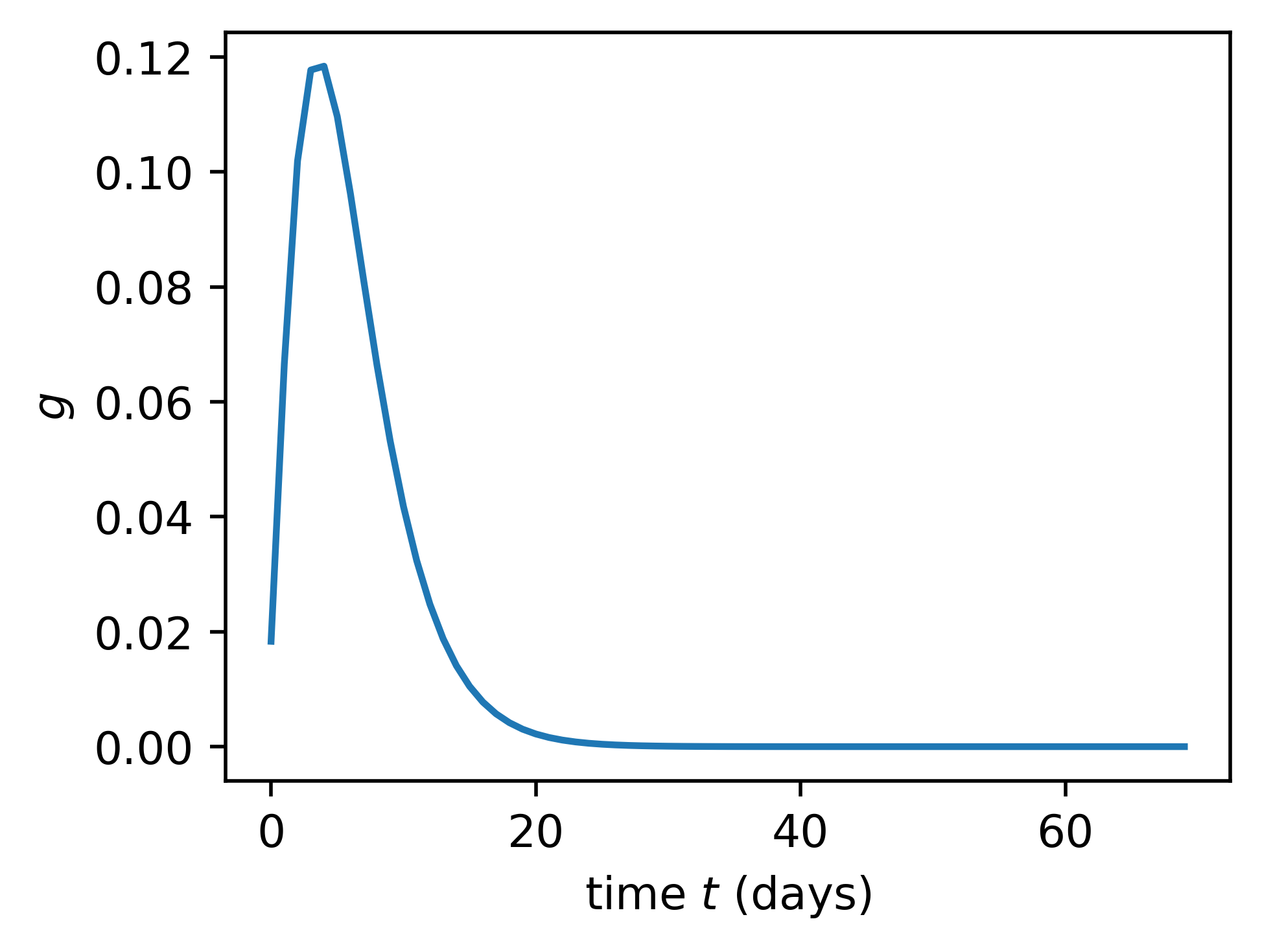
simulate an infection process from a negative binomial distribution with “number of successes” parameter and mean parameter specified in Eq. 6 – the mean of the semi-mechanistic model with generating distribution in Fig. 3 and
where is the maximum transmission rate. We consider linearly spaced values of in , and for each value, we set , which has the effect of keeping in the same ballpark for all values of .
-
5.
Finally, we simulate an observed time series – e.g. cases or deaths – according to Eq. 6 with and , for simplicity, so that for all .
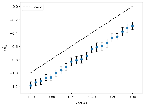
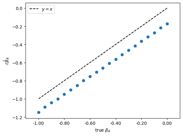
For each , we simulated 200 times series from the model, and for each, we obtained the MLEs of the ’s using the package freqepid, assuming negative binomial with semi-mechanistic model mean (Eq. 6) and reproduction number . Fig. 4 shows the averages of the 200 MLEs of for each true , along with 95% confidence intervals. There is phantom bias.
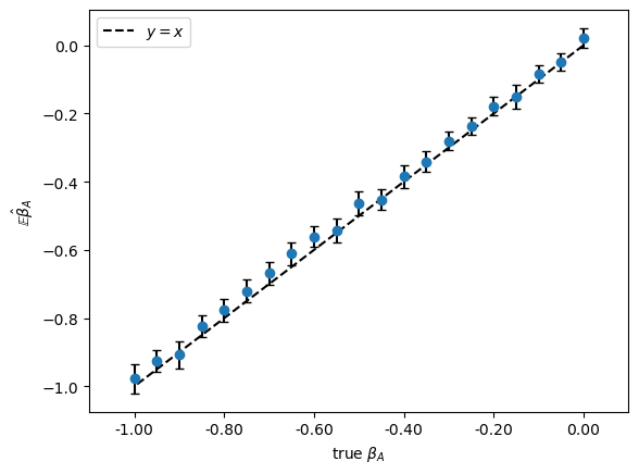
This bias is absent in the results under the same simulation conditions, except with set to zero, as shown in Fig. 7. This observation confirms that the bias in Fig. 4 is due to the presence of phantom variables.
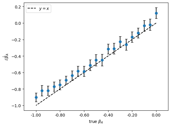
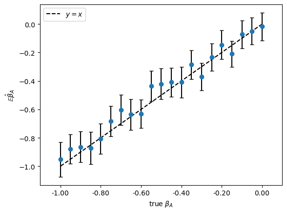
Next, we estimated using the estimating equation (Eq. 12) from the same simulation. For this, we employed the multiplicative semi-mechanistic model with the rate function . This model has closed-form expressions for both and its derivative , as derived in Examples Example 1 and Example 2. Using these results, we solved the estimating equation via Newton’s method. To address confounding, we modeled the propensity score for using a logistic regression based on , , and . From 200 i.i.d. estimates for each , we computed 95% confidence intervals, and Fig. 4 presents the results for 21 different true values of . These results demonstrate that the estimates obtained from the estimating equations are unbiased, even in the presence of phantom variables.
6.2 SEIR model simulated data
We demonstrate the same using the SEIR model in Eq. 2. First, we set , and , where the total population was set . Then for , we
-
1.
simulate phantoms from the same Gaussian random process as the previous example;
-
2.
sample confounders from a Gaussian distribution with variance and mean , where and ;
-
3.
generate binary interventions from a Bernoulli distribution with
where ;
-
4.
simulate an exposure process from a binomial distribution with number of trials and success probability
where . We consider linearly spaced values of in , and for each value, we set , which has the effect of keeping in the same ballpark for all values of .
Then, .
-
5.
simulate an infection process from a binomial distribution with number of trials and success probability .
Then, .
-
6.
Finally, we simulate an observed time series from a binomial distribution with number of trials and success probability .
Then, .
For each value of , we simulated 200 time series from the SEIR model. Since we do not have a developed method for estimating the MLE in this setting, we instead used a regressive approach to estimate the parameters. Specifically, for each iteration, we fit a binomial regression model:
where was included as a log-offset in the regression. This approximates the generation of the exposure process by using that when the right hand side is sufficiently small. Fig. 5 shows the average regressive estimates of over the 200 simulations for each true value of , along with the corresponding 95% confidence intervals. A phantom bias is evident in the estimates.
Next, we estimated using the estimating equation approach (Eq. 12) on the same simulated data. In this approach, the SEIR model was parameterized as . Since this model lacks a closed-form expression for and its derivative , we employed Monte Carlo approximations to compute them as described in Eq. 11 and Example 3, and solved the estimating equation using Newton’s method. To account for confounding, we modeled the propensity score of using a logistic regression model based on , , and . The 95% confidence intervals were derived from 200 independent estimates for each . Fig. 5 presents the results for 21 true values, showing that the estimates from the estimating equations are unbiased, even in the presence of phantom variables.
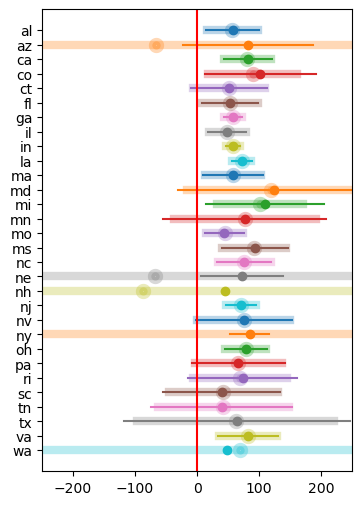
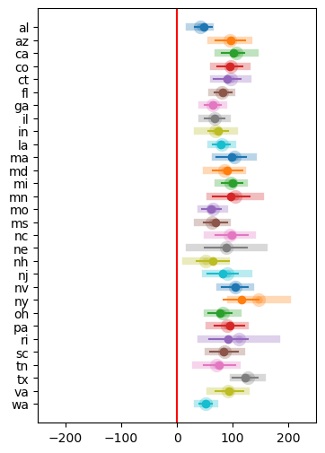
6.3 We Estimate the Causal Effect of Mobility on Covid-19 Transmission
We analyzed the effect of a mobility measure on Covid-19 death data for U.S. states, using the dataset described in Bong et al. (2023). The data are sourced from the Delphi repository at Carnegie Mellon University (delphi.cmu.edu), and consist of daily observations from February 15 to August 1, 2020 (168 days). The dataset includes state-level records of Covid-19 deaths, denoted as , and a mobility measure, “proportion of full-time work” (), which represents the fraction of mobile devices that spent more than six hours at a location other than their home during daytime (using SafeGraph’s full_time_work_prop). We focused on the 30 states that reported more than 20 deaths on at least one day and truncated the time series 30 days prior to reaching a total of 10 accumulated deaths, following the procedure outlined in Bhatt et al. (2022). A preprocessing step was used to correct for the weekend effect, which shows fewer deaths reported on Saturdays and Sundays (see Bong et al. (2023) for further details).
Figure 6 presents the estimates of from the estimating equation in Eq. 12, assuming the semi-parametric model (Eq. 6) for the 30 states. The faint thick lines show the point estimates and 95% confidence intervals, calculated separately for each state’s data. These estimates can be improved by borrowing strength across states using a frequentist approach based on the robust empirical Bayes shrinkage method introduced by Armstrong et al. (2022), and extended to multivariate parameters by Bong et al. (2023). The dark thin lines represent the shrinkage-adjusted estimates. We also compare these results with the maximum likelihood (ML) estimates from Bong et al. (2023), based on the same semi-parametric model, assuming negative binomial (NB) distributed death counts. All 30 states show differences in the estimates within the 95% confidence intervals between the estimating equation and ML approaches. Specifically, in 24 out of 30 states, the estimates from the estimating equation were lower than those from ML. This result is statistically significant, assuming a binomial probability of for the two methods yielding smaller estimates equally across all states (). This suggests the potential presence of a phantom effect, where the ML estimates may overestimate the global causal effect of mobility on Covid-19 deaths.
7 Conclusion
Augmenting an epidemic model to include an intervention variable is quite common. We have seen that such a model is best viewed as a model for counterfactual random variables. This makes it possible to use the model to answer causal questions about the effect of an intervention on an epidemic. We have argued that the best way to estimate the parameters in such a model is to use an appropriate estimating equation. Maximum likelihood and Bayesian methods are less useful as they are susceptible to certain biases due to latent variables. In particular, these methods can lead to rejecting the null hypothesis that there is no causal effect, even when the null is true.
There are many other subtleties involved in causal inference in the context of modeling epidemics. Yet the literature on combining methods of modern causal inference with epidemic modeling is sparse. This paper is meant as a first step in this direction.
References
- Andrews (1988) Donald WK Andrews. Laws of large numbers for dependent non-identically distributed random variables. Econometric theory, 4(3):458–467, 1988.
- Andrews (1991) Donald WK Andrews. An empirical process central limit theorem for dependent non-identically distributed random variables. Journal of Multivariate Analysis, 38(2):187–203, 1991.
- Armstrong et al. (2022) Timothy B Armstrong, Michal Kolesár, and Mikkel Plagborg-Møller. Robust empirical bayes confidence intervals. Econometrica, 90(6):2567–2602, 2022.
- Babino et al. (2019) Lucia Babino, Andrea Rotnitzky, and James Robins. Multiple robust estimation of marginal structural mean models for unconstrained outcomes. Biometrics, 75(1):90–99, 2019.
- Bates et al. (2022) Stephen Bates, Edward Kennedy, Robert Tibshirani, Valerie Ventura, and Larry Wasserman. Causal inference with orthogonalized regression: Taming the phantom. arXiv preprint arXiv:2201.13451, 2022.
- Bhatt et al. (2022) Samir Bhatt, Neil Ferguson, Seth Flaxman, Axel Gandy, Swapnil Mishra, and James A Scott. Semi-mechanistic bayesian modeling of covid-19 with renewal processes. Journal of the Royal Statistical Society, Series A, 2022.
- Bong et al. (2023) Heejong Bong, Valérie Ventura, and Larry Wasserman. Frequentist inference for semi-mechanistic epidemic models with interventions. arXiv preprint arXiv:2309.10792, 2023.
- Bonvini et al. (2022) Matteo Bonvini, Edward H. Kennedy, Valerie Ventura, and Larry Wasserman. Causal inference for the effect of mobility on COVID-19 deaths. The Annals of Applied Statistics, 16(4):2458 – 2480, 2022. doi: 10.1214/22-AOAS1599. URL https://doi.org/10.1214/22-AOAS1599.
- De Jong (1997) Robert M De Jong. Central limit theorems for dependent heterogeneous random variables. Econometric Theory, 13(3):353–367, 1997.
- De Jong and Davidson (2000) Robert M De Jong and James Davidson. Consistency of kernel estimators of heteroscedastic and autocorrelated covariance matrices. Econometrica, 68(2):407–423, 2000.
- Evans and Didelez (2024) Robin J Evans and Vanessa Didelez. Parameterizing and simulating from causal models. Journal of the Royal Statistical Society Series B: Statistical Methodology, 86(3):535–568, 2024.
- Gibson and Renshaw (1998) Gavin J Gibson and Eric Renshaw. Estimating parameters in stochastic compartmental models using markov chain methods. Mathematical Medicine and Biology: A Journal of the IMA, 15(1):19–40, 1998.
- Gourieroux and Monfort (1993) Christian Gourieroux and Alain Monfort. Simulation-based inference: A survey with special reference to panel data models. Journal of Econometrics, 59(1-2):5–33, 1993.
- Kermack and McKendrick (1927) William Ogilvy Kermack and Anderson G McKendrick. A contribution to the mathematical theory of epidemics. Proceedings of the royal society of london. Series A, Containing papers of a mathematical and physical character, 115(772):700–721, 1927.
- Lekone and Finkenstädt (2006) Phenyo E Lekone and Bärbel F Finkenstädt. Statistical inference in a stochastic epidemic seir model with control intervention: Ebola as a case study. Biometrics, 62(4):1170–1177, 2006.
- Mode and Sleeman (2000) Charles J Mode and Candace K Sleeman. Stochastic processes in epidemiology: HIV/AIDS, other infectious diseases and computers. World Scientific, 2000.
- Newey et al. (1987) Whitney K Newey, Kenneth D West, et al. A simple, positive semi-definite, heteroskedasticity and autocorrelation consistent covariance matrix. Econometrica, 55(3):703–708, 1987.
- Robins (1986) James Robins. A new approach to causal inference in mortality studies with a sustained exposure period—application to control of the healthy worker survivor effect. Mathematical modelling, 7(9-12):1393–1512, 1986.
- Robins (2000) James M Robins. Marginal structural models versus structural nested models as tools for causal inference. In Statistical models in epidemiology, the environment, and clinical trials, pages 95–133. Springer, 2000.
- Robins and Wasserman (1997a) James M Robins and L Wasserman. Estimation of effects of sequential treatments by reparameterizing directed acyclic graphs. In Proceedings of the Thirteenth Conference on Uncertainty in Artificial Intelligence, pages 409–420. Morgan Kaufmann, 1997a.
- Robins and Wasserman (1997b) James M Robins and Larry Wasserman. Estimation of effects of sequential treatments by reparameterizing directed acyclic graphs. In Proceedings of the Thirteenth conference on Uncertainty in artificial intelligence, pages 409–420, 1997b.
Appendix