Why Go Full? Elevating Federated Learning
Through Partial Network Updates

Abstract

Federated learning is a distributed machine learning paradigm designed to protect user data privacy, which has been successfully implemented across various scenarios. In traditional federated learning, the entire parameter set of local models is updated and averaged in each training round. Although this full network update method maximizes knowledge acquisition and sharing for each model layer, it prevents the layers of the global model from cooperating effectively to complete the tasks of each client, a challenge we refer to as layer mismatch. This mismatch problem recurs after every parameter averaging, consequently slowing down model convergence and degrading overall performance. To address the layer mismatch issue, we introduce the FedPart method, which restricts model updates to either a single layer or a few layers during each communication round. Furthermore, to maintain the efficiency of knowledge acquisition and sharing, we develop several strategies to select trainable layers in each round, including sequential updating and multi-round cycle training. Through both theoretical analysis and experiments, our findings demonstrate that the FedPart method significantly surpasses conventional full network update strategies in terms of convergence speed and accuracy, while also reducing communication and computational overheads.

1 Introduction

Federated learning is a machine learning framework that protects data privacy, which has attracted widespread attention from researchers in recent years (McMahan et al., 2017; Kairouz et al., 2019; Li et al., 2019). In traditional federated learning, after receiving the global model sent by the server, each client uses their local data to update the entire model parameters set for several iterations; then, the server averages the updated models to obtain a new global model and broadcasts it to all clients, starting the next training round.

Although this paradigm has been successful in many scenarios (Hard et al., 2018; Rieke et al., 2020), its convergence speed and ultimate performance are often lower than those of centralized schemes (McMahan et al., 2017; Zou et al., 2023), even when data across clients are independently and identically distributed (i.i.d.). This suggests that while full network updates and sharing enrich each model layer with more knowledge, they also introduce potential negative effects on final performance. To further investigate the underlying reason, we conduct an experiment to visualize the update step sizes during each iteration. Typically, in centralized learning, the update step sizes of the model show a downward trend, indicating that the model is gradually converging. However, in federated learning, as shown in Fig. 1a, the update step sizes significantly increase after each parameter averaging. This suggests that after averaging, the gradients calculated by subsequent layers become particularly large, indicating inadequate cooperation among layers within the global model, a phenomenon we term as layer mismatch. The cause of this issue is illustrated in Figure 2a. The middle section of the figure depicts the local models of each client, which have undergone sufficient local training. Within these local models, the layers cooperate effectively, demonstrating match. However, upon aggregating the parameters of each layer, the averaged layers may struggle to maintain this cooperation, resulting in mismatch. Such layer mismatch could lead to two problems: firstly, the final global model in federated learning may not converge to the optimal point of the global loss function, thereby negatively affecting performance. Secondly, the overall federated learning process may continually experiencing disruption due to mismatch by the server, substantially hampering training efficiency.

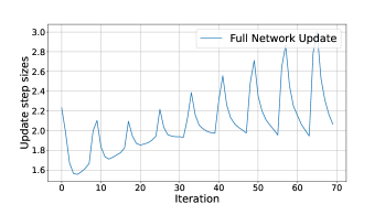
(a) Update step sizes of traditional federated learning with full network updates.

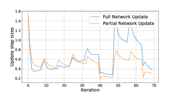
(b) Update step sizes comparison between full network updates and partial network updates.

Figure 1: Update step sizes for each iteration. The experiment uses the ResNet-8 model with 20,000 CIFAR-100 images distributed in an i.i.d. manner across 40 clients.

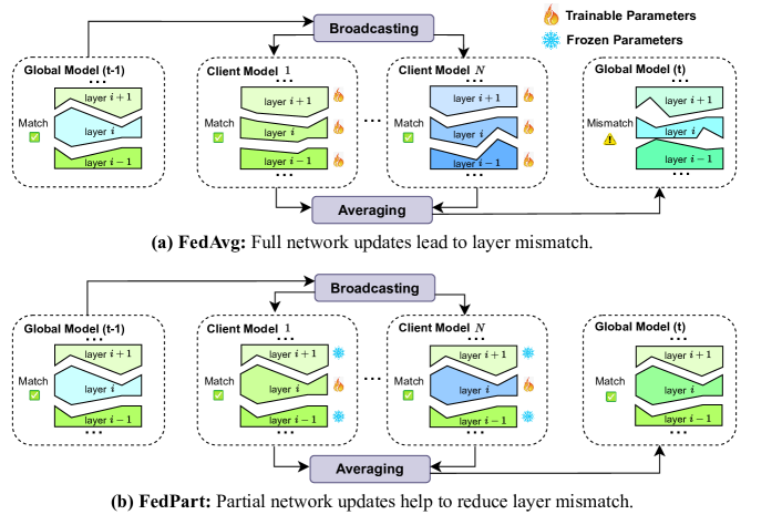
Figure 2: Mechanism for layer mismatch in FedAvg and FedPart.

To address the aforementioned problems, we propose FedPart, which employs partial network updates. Our main motivation is illustrated in Fig. 2b. In this toy example, we assume that only the $i$-th layer of the network is trainable in the current round. During local training of each client, the $i$-th layer can naturally align with other frozen parameters. These untrainable layers act as anchors, constraining the update direction of the $i$-th layer. This makes the averaged layers more likely to align with other layers. To validate this approach, we conduct experiments and visualize the results in Figure 1b. The curves clearly demonstrate that partial network updates significantly reduce the increase in update step sizes after averaging, thereby affirming their effectiveness in mitigating layer mismatch.

However, as a trade-off, training and transmitting only a portion of the parameters at a time might limit the efficiency of knowledge learning and sharing. After thorough analysis, we identify that the solution to this problem lies in the strategy for selecting trainable parameters. Therefore, we carefully design a strategy for selecting trainable parameters in FedPart, drawing on two key principles. The first principle is sequential updating. We train the network layers sequentially, from shallow to deep, one layer at a time. This design is based on the observation that the shallower layers of a neural network typically converge to their final parameters faster than the deeper ones (Raghu et al., 2017). To maintain consistency with this inherent order, we apply a similar sequential strategy in layer selection. The second principle is the multi-round cycle training strategy. Our method emphasizes the importance of repeating the process of training from shallow layers to deep layers multiple times. During the original full network updates, shallow layers often learn low-level features, while deep layers learn high-level semantic features (Zeiler and Fergus, 2014; Erhan et al., 2009). To preserve this property, inspired by the idea of Block Coordinate Descent (BCD) (Poczos and Tibshirani, ), we propose the multi-round cycling training method to retain this characteristic to the greatest extent.

In addition, FedPart also features computation and communication efficiency, which makes it highly suitable for edge computation scenarios (Wang et al., 2019a, b; Abreha et al., 2022). This is because FedPart only needs to train a part of the neural network at each training round, thereby significantly reducing the computational overhead of each client in each iteration. At the same time, since clients only need to upload and download the parts of the model that need updating, the amount of parameters to be transmitted is also greatly reduced.

To validate the effectiveness of FedPart, we conduct explorations from both theoretical and experimental perspectives. Theoretically, we demonstrate that FedPart has a superior convergence rate under non-convex settings compared to FedAvg. Experimentally, we perform extensive evaluations on various datasets and model architectures. The results indicate that the FedPart method significantly improves convergence speed and final performance (e.g., an improvement of 24.8% on Tiny-ImageNet with ResNet-18), while also reducing both communication overhead (by 85%) and computational overhead (by 27%) simultaneously. Furthermore, our ablation experiments highlight the individual contributions of the proposed strategies in enhancing the overall performance of FedPart. We also include comprehensive visualization experiments to demonstrate the internal rationality of FedPart. In summary, the contributions of this paper are as follows:

• We observe the issue of layer mismatch in federated learning, caused by updating and aggregating all parameters in each training round. This phenomenon can potentially impact the model’s convergence speed and overall performance.

• To mitigate the effects of layer mismatch, we introduce FedPart, which implements partial network updates. Additionally, we develop corresponding strategies for selecting trainable parameters.

• We analyze the convergence rate of FedPart in a non-convex setting, demonstrating its theoretical advantages over full network updates.

• We perform extensive experiments, showing that FedPart achieves significant improvements across multiple evaluation metrics compared to the full network update scheme. Additionally, ablation and visualization experiments help to further understand the rationality of FedPart.

2 Related Work

Currently, researches on partial parameter training or aggregation in federated learning has seen some applications, which can be broadly categorized into three types:

Train all parameters, aggregate partial parameters. Also known as personalized federated learning, this approach involves each client training all parameters but only aggregating some of them (Tan et al., 2022). For example, FedPer (Arivazhagan et al., 2019) and FedBN (Li et al., 2021b) personalizes classification and batch-normalization layers respectively, FedRoD (Chen and Chao, 2021) applies both global and local classifier heads. Other works may only upload a low-rank space of parameter matrices (Wang et al., 2023; Wu et al., 2024a). Although these methods achieve impressive results in data-heterogeneous scenarios, they usually exhibit performance degradation when datasets across clients are distributed in an i.i.d. manner. Additionally, these methods do not reduce computational overhead and, and the reduction in communication overhead is also relatively minimal since the personalized parts are usually small.

Train partial parameters, aggregate all parameters. This category refers to each client training a different part of the model, with a general update to the entire model during aggregation. For example, PVT (Yang et al., 2022) and FedPT (Sidahmed et al., 2021) strategically assigns specific model layers to each client, Federated Dropout (Caldas et al., 2018) and FedPMT (Wu et al., 2023) randomly assign a neurons in different layers to clients, HeteroFL (Diao et al., 2020) and FjORD (Horvath et al., 2021) deterministically decide a trainable subnetwork based on client computational power, FedRolex (Alam et al., 2022) further introduces a sliding window method, and CoCoFL (Pfeiffer et al., 2022) introduces a quantization technique for overhead reduction. The core goal of these methods is generally to reduce client overhead, especially focusing on dynamically utilizing the varying computational powers for clients. However, compared to full network updates, these methods often result in performance degradation and slower convergence speed.

Progressive Training. This approach starts with a small model and gradually increases its size until the entire network is trained (Rusu et al., 2016). This training paradigm has gain attention in the field of federated learning as its efficiency in reducing resource consumption (e.g., ProgFed (Wang et al., 2022) and ProFL (Wu et al., 2024b)). However, because these methods eventually train a full model, they are not able to solve the layer mismatch problem. Moreover, while they aim to reduce resource consumption, they often result in performance loss compared to full network training. To the best of our knowledge, our FedPart is the first to simultaneously boost convergence accuracy and efficiency.

3 Method

Generally speaking, FedPart is based on partial network updates, which trains and aggregates only few layers of the global network model for each training round. At the beginning of each training round that requires partial network update, the server first determines which layers need to be trained and sends this information to all clients. Subsequently, each client trains the corresponding layers, transmitting them to the server for aggregation, and the server broadcasts the averaged results to each client for next training round. We elaborate on two crucial elements in the subsequent subsections: partial network updates and the strategy for selecting trainable layers.

3.1 Partial Network Updates

The partial network updates involve training and aggregating only few layers of the global network model in each later communication rounds. Specifically, we partition the layers of global model into trainable ones and frozen ones. For each training iteration $t$ and client $i$, the optimization objective is: $\mathop{\arg\min}_{w_{i}^{t}}\mathbb{E}_{x\sim\mathbf{D_{i}}}[\mathcal{L}(x|\hat{w_{i}^{t}},\tilde{w}_{i}^{t})],$ where $\hat{w_{i}^{t}}$ and $\tilde{w}_{i}^{t}$ respectively denotes parameters of trainable and non-trainable layers, $\mathbf{D_{i}}$ represents the local data distribution of client $i$ and $\mathcal{L}(\cdot)$ refers to the loss function. To optimize this objective, we adopt the following gradient descent formula:

$$w_{i}^{t+1}=w_{i}^{t}-\gamma*S_{i}^{t}\odot\nabla_{w_{i}^{t}}\mathcal{L}(x|w_{i}^{t}),\quad x\sim\mathbf{D_{i}}.$$ (1)

Here, $w_{i}^{t}\triangleq\{\hat{w}_{i}^{t},\tilde{w}_{i}^{t}\}$ represents the total parameter set, $\gamma$ is the learning rate, $S_{i}^{t}$ is a binary mask that selectively enables updates only for trainable parameters and $\odot$ denotes element-wise product. After performing several local training iterations, the parameters of these selected layers are sent to the server and globally averaged at iteration $T$: $\bar{w}_{T}=\frac{1}{N}\sum_{i=1}^{N}w_{i}^{T},$ where $N$ represents the number of clients. In the formula mentioned above, for simplicity of formulation, we aggregate and calculate the gradient for all parameters. However, in practical implementation, we only update and transmit the trainable parts, thereby significantly reducing the computational and communication costs.

3.2 Strategy for Selecting Trainable Layers

Training only a subset of parameters in each round may restrict the efficiency of knowledge learning and sharing. Our main aim in designing the strategy for selecting trainable layers is to mitigate this limitation. As illustrated in Fig.3, following the initial full network updates, we train parameters layer by layer from the shallowest to the deepest. Subsequently, we cycle back to the shallowest layer and periodically repeat this process. This strategy encompasses the following two key principles:

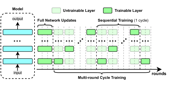
Figure 3: Strategy for selecting trainable layers.

Sequential updating. This principle refers to training model layers in sequence, from shallow to deep layers one at a time. Our motivation is that the convergence of neural network exhibits a natural intrinsic order, with shallower layers typically converging earlier than deeper ones (Raghu et al., 2017). By updating partial network in accordance with this inherent training order, we can mirror the convergence process of full network updates, thus maintaining the training efficiency.

Multi-round cycle training. This principle refers to repeating the process of updating the neural network layers from shallow to deep multiple times. We illustrate our motivation with an example: in a fully trained neural network, shallow layers primarily focus on low-level semantic features (such as the edges in images), while deeper layers focus on higher-level semantic features (such as the main objects in images). However, during partial network updates, because the deeper layers are initially non-trainable, shallow layers are forced to learn complex high-level semantic features, which disrupts the original information hierarchy in the neural network. Through multi-round cycle training, we return to the shallow layers after training the deep layers. This strategy can reduce the burden on the shallow layers and approximate the final effect of full network updates.

3.3 Convergence Analysis for FedPart

To analyze the convergence of FedPart, we first introduce some definitions and notations. Let each client use a uniform loss function $\mathcal{L}(x|w)$ with parameters $w$, for the data $x$ to calculate the loss function value, $f_{i}(w)=\mathbb{E}_{x\sim\mathbf{D_{i}}}[\mathcal{L}(x|w)]$ which is the expected loss function of client $i$. In this setting, the overall optimization goal of federated learning can be written as the sum of the expected loss functions of each client, that is: $f(w)=\frac{1}{N}\sum_{i=1}^{N}f_{i}(w)$. Additionally, for notational simplicity, we denote the parameters of the $i$-th client at time $t$ as $w_{i}^{t}$, the computed stochastic gradient vector as $G_{i}^{t}$, and the average of all client models at time $t$ as $\bar{w}^{t}$.

To represent partial network updates, we add a binary matrix $S_{i}^{t}$ as a mask for each update process of each client. To keep consistency with the methods section, we assume that for each mask $S_{i}^{t}$, $\frac{1}{M}$ of the elements are 1, and the rest are 0. Before proving the convergence of our FedPart under non-convex conditions, we first propose three necessary assumptions:

Assumption 1: The expected loss function of any client is L-smooth, namely:

$$||\nabla f_{i}(w)-\nabla f_{i}(u)||\leq L||w-u||,\forall i,w,u.$$ (2)

Assumption 2: The variance and second-order moments of the gradients are bounded, that is:

$$\mathbb{E}_{x\sim\mathbf{D_{i}}}[||\nabla\mathcal{L}(x|w)-\nabla f_{i}(w)||^{2}] \leq\sigma^{2},\forall i,w,x\in\mathbf{D_{i}},$$

$$\mathbb{E}_{x\sim\mathbf{D_{i}}}[||\nabla\mathcal{L}(x|w)||^{2}] \leq G^{2},\forall i,w,x\in\mathbf{D_{i}}.$$

Assumption 3: The variance of the gradients is approximately equal under all permissible masks:

$$\frac{\mathbb{E}_{x\sim\mathbf{D_{i}}}[||S_{1}\odot(\nabla\mathcal{L}(x|w)-\nabla f_{i}(w))||]}{\mathbb{E}_{x\sim\mathbf{D_{i}}}[||S_{2}\odot(\nabla\mathcal{L}(x|w)-\nabla f_{i}(w))||]}\leq k,\forall i,w,x\in\mathbf{D_{i}},S_{1},S_{2}.$$ (3)

The first two assumptions are common in the literature, ensuring certain necessary characteristics of the loss function. The third assumption ensures that the specific choice of the mask matrix does not have too much impact on the final update variance, as long as the mask meets the requirements. A further discussion about the third assumption can be found in Appendix G.

Based on these assumptions, we can analyze the convergence of FedPart. In terms of the approximate convergence rate, we maintain consistency with related literature (Alistarh et al., 2017; Lian et al., 2017; Ghadimi and Lan, 2013), using the average magnitude of the expected gradient over iterations, and finally obtain the following theorem form:

Theorem: Under assumptions 1-3, with the total number of clients as $N$, and all parameters divided into $M$ groups of trainable parameters, the convergence rate of FedPart satisfies:

$$\frac{1}{T}\sum_{t=1}^{T}\mathbb{E}[||S_{i}^{t}\odot\nabla f(\bar{w}^{t-1})||^{2}]=O(\frac{1}{\sqrt{MNT}}),$$ (4)

where $\odot$ denotes element-wise product. A detailed proof of this theorem is provided in Appendix B. The results show that compared to the convergence rate of full network updates $O(\frac{1}{\sqrt{NT}})$ (Yu et al., 2019), FedPart’s convergence performance is significantly better. This advantage becomes more pronounced as the choice amount of partial parameters per instance is reduced, which aligns with our original intention to reduce layer mismatch. However, it should be noted that convergence analysis can only indicate the difficulty of converging to a stationary point, and cannot measure the model’s performance after convergence. Therefore, in practice, it is not advisable to indiscriminately reduce the amount of parameters trained each time.

3.4 Analysis for Communication and Computational Cost

Communication Cost. Suppose FedPart divides all layers into $M$ groups, and only one group is trained during each partial training session, with one communication round for each group. Then, the communication costs of FedPart will be $\frac{1}{M}$ of the original costs. This significant reduction can be explained as follows: Assume the communication cost of transmitting the complete model is $C$. By comparing the total communication cost for updating all parameters $Comm_{FNU}$ against the cost for updating only a subset of parameters $\boldsymbol{Comm_{PNU}}$ across one training cycle, we can derive:

$$\frac{\boldsymbol{Comm_{PNU}}}{Comm_{FNU}}=\frac{C}{M*C}=\frac{1}{M}.$$ (5)

Computational Cost. Assume computational costs are the same across all layers, our method in the partial network update phase can reduce the overall computational expense by $\frac{1}{3}$. The primary reason for this reduction is that in FedPart, it is unnecessary to compute gradients for the layers preceding the trainable parameters. To analyze this quantitatively, suppose the total overhead for both forward and backward propagation in a complete model satisfies $D_{tot}=D_{for}+D_{bak}$. The ratio of computational costs over a single training cycle can then be formulated as

$$\frac{\boldsymbol{Comp_{PNU}}}{Comp_{FNU}}=\frac{M*D_{for}+\sum_{i=1}^{M}\frac{i*D_{bak}}{M}}{M*D_{for}+M*D_{bak}}=\frac{M*D_{for}+\sum_{i=1}^{M}\frac{(M+1)*D_{bak}}{2M}}{M*D_{for}+M*D_{bak}}.$$

Given the nature of the backward propagation formulas, it is often approximated in the literature that the computational cost of backward propagation is about twice that of forward propagation (Rasley et al., 2020; Hobbhahn and Sevilla, 2021). Therefore, the above equation can be rewritten as:

$$\frac{\boldsymbol{Comp_{PNU}}}{Comp_{FNU}}\approx\frac{M*D_{for}+{(M+1)*D_{for}}}{M*D_{for}+2M*D_{for}}\approx\frac{2}{3}$$ (6)

4 Experiments

In the experimental setup, we primarily choose 40 clients, with local epochs to be 8. We test the global model on a balanced set. Unless specifically stated otherwise, the training datasets across all clients are independently and identically distributed (i.i.d.). We utilize the Adam optimizer (Kingma and Ba, 2014) with a learning rate of 0.001, which is determined to be the optimal learning rate. Consistent with prior references (Li et al., 2021b; Chen et al., 2022), we refrain from uploading local statistical information during model aggregation. Each experiment is conducted three times with different random seeds to ensure robustness. The experimental results for additional scenarios, including learning-rate tuning and client sampling, are presented in Appendix F.

When choosing experimental metrics, we employ three distinct measures to capture different facets of the benefits. These metrics include: Best Acc., which represents the ultimate accuracy achieved in classification tasks; Comm., indicating the total upstream transmission volume required by each client for a given training round (in GB); and Comp., which illustrates the total floating-point computation required by each client (in TFLOPs). All experiments are conducted on a server equipped with 8×A100 GPUs, and we provide the complete source code in our supplementary material.

4.1 Main Properties

Comparison with full network updates. We apply the FedPart method to three classic federated learning algorithms: FedAvg (McMahan et al., 2017), FedProx (Sahu et al., 2018), and FedMOON (Li et al., 2021a), and compare the results with their full network updates (FNU) counterparts. We utilize ResNet-8 (He et al., 2016) (detailed in Appendix A) and update only one layer in each two consecutive training rounds (denoted as 2 R/L). Additionally, we insert five rounds of full network training between each cycle in our FedPart. We conduct experiments on the CIFAR-10 (Krizhevsky et al., 2010), CIFAR-100 (Krizhevsky et al., 2009), and TinyImageNet (Le and Yang, 2015) datasets.

Table 1: Performance of FL algorithms with full network and partial network updates.

Data	C	FedAvg		FedProx		FedMoon		Comm.		Comp.
		FNU	FedPart	FNU	FedPart	FNU	FedPart	FNU	FedPart	FNU	FedPart
CIF AR- 10	1	56.0 (±1.1)	57.7 (±0.5)	54.4 (±2.1)	57.5 (±0.6)	58.9 (±0.5)	57.8 (±0.4)	4.83	1.35	4.38	3.21
	2	58.6 (±1.6)	60.2 (±0.4)	60.2 (±1.5)	59.9 (±0.5)	61.1 (±0.1)	59.4 (±0.2)	9.65	2.70	8.76	6.43
	3	59.6 (±1.7)	61.7 (±0.3)	62.3 (±0.7)	61.3 (±0.1)	62.3 (±0.4)	59.8 (±0.1)	14.5	4.05	13.2	9.64
	4	60.7 (±1.3)	62.8 (±0.2)	62.8 (±1.1)	62.3 (±0.1)	62.3 (±0.4)	60.5 (±0.6)	19.3	5.40	17.5	12.9
CIF AR- 100	1	30.9 (±0.4)	31.0 (±0.5)	30.6 (±0.3)	30.9 (±0.5)	31.0 (±0.5)	30.9 (±0.4)	4.92	1.38	4.39	3.22
	2	32.9 (±0.3)	34.8 (±0.5)	33.6 (±0.5)	34.7 (±0.4)	33.2 (±0.9)	35.1 (±0.4)	9.65	2.75	8.78	6.44
	3	34.3 (±0.2)	36.1 (±0.5)	34.5 (±0.5)	36.7 (±0.4)	34.6 (±1.1)	36.5 (±0.6)	14.8	4.13	13.2	9.66
	4	35.6 (±0.3)	37.0 (±0.6)	35.8 (±0.2)	37.1 (±0.4)	35.0 (±1.0)	37.2 (±0.6)	19.7	5.51	17.6	12.9
	5	35.6 (±0.3)	37.2 (±0.7)	36.2 (±0.5)	37.5 (±0.2)	35.4 (±0.8)	37.6 (±0.5)	24.6	6.88	21.9	16.1
Tiny- Imag eNet	1	15.6 (±0.6)	17.1 (±0.2)	15.8 (±0.4)	16.8 (±0.2)	17.5 (±0.6)	17.3 (±0.3)	5.02	1.40	17.5	12.9
	2	17.0 (±0.8)	20.3 (±0.1)	17.2 (±1.0)	20.1 (±0.2)	17.5 (±0.6)	20.5 (±0.0)	10.0	2.81	35.1	25.7
	3	17.6 (±0.4)	20.8 (±0.2)	18.0 (±0.5)	20.7 (±0.1)	18.4 (±0.8)	21.1 (±0.1)	15.1	4.21	52.6	38.6
	4	17.7 (±0.4)	21.1 (±0.1)	18.2 (±0.7)	21.2 (±0.1)	18.4 (±0.8)	21.5 (±0.1)	20.1	5.62	70.1	51.4
	5	17.7 (±0.4)	21.4 (±0.2)	18.4 (±0.8)	21.5 (±0.2)	18.4 (±0.8)	21.7 (±0.1)	25.1	7.02	87.7	64.3

The results in Table 1 show that our FedPart method demonstrates rapid convergence and consistently outperforms traditional FNU methods across all training cycles C, ultimately achieving significantly higher accuracy (e.g., improving FedAvg on Tiny-ImageNet by 21%). At the same time, its communication and computational costs are only 28% and 73% of those required by FNU. Furthermore, we observe that in some scenarios, the performance improvements of other federated learning algorithms even surpass those observed with FedAvg. This demonstrates that the layer mismatch problem we address is fundamentally different from issues tackled by previous works, and thus the performance enhancements they provide are independent of each other. This is a highly desirable property. However, our results on CIFAR-10 are less impressive. This suggests that in simpler datasets, the primary issue might be the client drift problem explored in previous studies, whereas the layer mismatch problem becomes more prominent in complex datasets.

Table 2: Performance of FedPart for ResNet-18.

Data	C	FedAvg-FNU			FedAvg-FedPart
		Best Acc.	Comm.	Comp.	Best Acc.	Comm.	Comp.
CIFAR- 10	1	59.4 (±1.5)	82.1	11.2	53.5 (±0.5)	12.2	8.19
	2	61.4 (±0.1)	164	22.3	57.5 (±0.6)	24.5	16.4
	3	61.7 (±0.2)	246	33.5	59.2 (±0.4)	36.7	24.6
CIFAR- 100	1	30.4 (±0.4)	82.5	11.2	27.8 (±0.5)	12.3	8.20
	2	31.9 (±0.6)	165	22.4	31.6 (±0.4)	24.6	16.4
	3	32.0 (±0.5)	247	33.5	33.4 (±0.4)	36.8	24.6
Tiny- ImageNet	1	13.7 (±0.2)	82.8	44.7	12.0 (±0.2)	12.3	32.8
	2	13.7 (±0.2)	166	89.4	15.1 (±0.3)	24.7	65.5
	3	13.7 (±0.2)	248	134	17.1 (±0.2)	37.0	98.3

FedPart with deeper models. To evaluate the effectiveness of FedPart with deeper networks, we conduct experiments on ResNet-18 (detailed in Appendix A). This presents a more challenging scenario, as the proportion of trainable parameters significantly decreases in each round. Our experimental setup also follows the 2 R/L pattern, with five additional full network updates inserted between cycles. The results, displayed in Table 2, show that in deeper networks, FedPart not only maintains its advantages in terms of convergence speed and accuracy but also offers even more substantial reductions in communication and computational costs (by 85% and 27% compared to full network updates).

Table 3: Performance of FedPart on NLP datasets.

Data	C	FedAvg-FNU			FedAvg-FedPart
		Best Acc.	Comm.	Comp.	Best Acc.	Comm.	Comp.
AG News	1	91.4 (±0.3)	22.3	5.58	91.1 (±0.2)	7.43	4.16
	3	92.0 (±0.2)	66.9	16.7	91.5 (±0.2)	22.3	12.5
	5	92.1 (±0.3)	106	27.9	92.0 (±0.3)	37.2	20.8
Sogou News	1	94.2 (±0.2)	51.8	5.58	93.8 (±0.2)	17.3	4.16
	3	94.3 (±0.2)	155	16.7	94.3 (±0.2)	51.8	12.5
	5	94.4 (±0.2)	259	27.9	94.4 (±0.2)	86.3	20.8

FedPart for language modality. We also extend the FedPart method to the field of natural language processing and evaluate it on AGnews and SogouNews (Zhang et al., 2015) datasets. We choose the transformer architecture (Vaswani et al., 2017) for experiments. As shown in Table 3, the results indicate that FedPart performs well on language tasks, not only maintaining comparable performance as FNU, but also reducing communication and computational overhead by 66% and 25%, respectively. This demonstrates the method’s extensibility.

FedPart under data heterogeneity. We also evaluate the performance of FedPart under scenarios involving data heterogeneity. The results in Table 5 show that our FedPart consistently improve final performance(e.g., an improvement of 3.4% on Tiny-ImageNet) in the presence of data heterogeneity. However, the extent of performance improvement is relatively smaller. This suggests that client drift (Karimireddy et al., 2020) may have a more pronounced negative impact on our method. We also conduct experiments with extreme data heterogeneity ($\alpha=0.1$) in Appendix F.3.

Table 4: Performance of FedPart under data heterogeneity (Dirichlet, $\alpha=1$).

Dataset	C	FedAvg-FNU	FedPart
CIFAR- 10	2	57.7 (± 0.7)	57.8 (± 0.4)
	3	59.2 (± 0.7)	59.2 (± 0.4)
	4	60.4 (± 1.1)	60.7 (± 0.4)
	5	60.4 (± 1.1)	61.4 (± 0.4)
CIFAR- 100	2	33.1 (± 0.4)	34.4 (± 0.1)
	3	34.3 (± 0.6)	35.8 (± 0.2)
	4	34.9 (± 0.6)	36.8 (± 0.1)
	5	35.2 (± 0.5)	37.4 (± 0.1)
Tiny- ImageNet	2	16.9 (± 0.3)	19.8 (± 0.4)
	3	17.4 (± 0.1)	20.3 (± 0.1)
	4	17.4 (± 0.1)	20.4 (± 0.1)
	5	17.4 (± 0.1)	20.8 (± 0.3)

Table 5: Performance of FedPart with different training rounds per layer.

Dataset	R/L	r=15	r=25	r=35	r=45	r=55	r=65
CIFAR- 10	1	58.06	59.35	60.06	60.56	61.12	61.21
	2	56.85	58.80	58.80	60.46	60.46	61.25
	4	56.17	58.76	59.60	59.60	59.60	59.60
	10	48.22	54.65	57.40	57.40	59.03	59.03
CIFAR- 100	1	28.10	29.86	31.25	32.17	32.60	33.09
	2	24.47	30.07	30.07	32.53	32.53	33.59
	4	23.56	26.26	28.19	32.01	32.01	32.01
	10	22.83	23.51	26.04	26.43	29.21	30.94
Tiny- ImageNet	1	14.37	16.33	18.02	19.27	19.88	20.18
	2	11.32	16.00	16.00	19.25	19.25	20.69
	4	9.09	11.44	15.21	17.89	17.89	17.89
	10	11.33	12.03	12.03	12.03	12.03	16.16

4.2 Ablation Study

Training rounds per layer. In our FedPart, the training rounds per layer (denoted as $R/L$) is an important hyperparameter. A larger R/L value means more thorough training in each cycle, but it also results in a decrease in the number of cycles within the same number of training rounds. We explore the performance of FedPart under different R/L. From the results in Table 5, when $R/L=1$, the outcome shows limited final performance due to insufficient training for each layer. However, further increasing the R/L value not only fails to improve the final performance but also reduces the convergence speed. In extreme cases, when $R/L=10$, only one cycle is conducted overall, significantly impacting both the convergence speed and the final accuracy. This indicates that generally, increasing the number of cycles is more reasonable than extending their duration. This aligns with the motivation behind our proposal of multi-cycling training.

Table 6: Impact of the warm-up rounds.

Dataset	State	0 init.	5 init.	60 init.
CIFAR- 10	bef.	0	41.56	58.92
	aft.	58.48	61.25	66.18
CIFAR- 100	bef.	0	20.38	34.16
	aft.	29.53	33.59	36.65
Tiny- ImageNet	bef.	0	9.11	16.25
	aft.	16.81	20.69	19.99

Table 7: Impact of training sequences.

Dataset	C	Seq.	Rev.	Ran.
CIFAR- 10	1	58.80	58.53	59.62
	2	60.46	59.76	59.97
	3	61.25	60.19	60.23
CIFAR- 100	1	30.07	27.84	29.58
	2	32.53	29.41	30.92
	3	33.59	31.79	31.44
Tiny- ImageNet	1	16.00	13.15	15.91
	2	19.25	15.62	17.71
	3	20.69	18.33	18.99

Rounds of initial warm-up updates. To explore the impact of the duration of the initial full network updates phase (i.e. warm-up stage), we conduct experiments with this stage set to lengths of 0, 5, and 60. In Table 7, the term state refers to the period before or after partial network updates, which follow the warm-up phase. The experimental results clearly show that initial full network updates is crucial to the final model’s accuracy. However, extending the full network update phase yields diminishing returns. However, even when the model is trained with FNU until no further accuracy improvement is observed (60 init.), utilizing FedPart still enhances the model’s accuracy. This confirms FedPart’s capability to improve the convergence of the final global model and reduce layer mismatch.

Different orders for selecting trainable layers. We experiment with three different orders for selecting trainable parameters: sequential, reverse, and random. Sequential is the default configuration of FedPart, selecting layers from shallow to deep. In contrast, the reverse sequence selects layers from deep to shallow, while the random sequence selects layers randomly in each round. The results of the experiments are depicted in Table 7, demonstrating that the effectiveness of the three methods ranks as: sequential > reverse > random. This aligns with the intrinsic convergence order of neural networks and meets our experimental expectations.

4.3 Visualization Results

In this section, we conduct experiments to demonstrate why our proposed parameter selection strategy can enhance final performance, and what the impact of layer-wise information exchange has on privacy. Our experiments are based on ResNet-8 and the CIFAR-100 dataset. We analyze the models obtained from four different methods: 1) FedAvg-100, which represents training with full network for 100 rounds; 2) FedPart(No Init. 1C), which represents using FedPart for one cycle without initial full network updates; 3) FedPart(1C), which involves initial full network updates followed by one cycle of FedPart training; 4) FedPart(5C), which involves initial full network updates followed by five cycles of FedPart training. The visualization results are as follows.

Activation maximization visualization. Activation maximization (Erhan et al., 2009) involves finding an input that maximizes a specific activation value within a neural network, reflecting the feature patterns the neuron focuses on. We use this method to explore the visual patterns captured by different models and measure their similarity using SSIM (Structural Similarity Index Measure) (Hore and Ziou, 2010). The results in Table 9 show that, without initial full network updates and multiple cycles, the features captured by the FedPart model significantly differ from those of the FedAvg model. However, this discrepancy decreases after applying our layer-selection strategy, suggesting that the model better recognizes the hierarchical nature of different semantic information, thus enhancing its performance. Additional visual results are provided in Appendix C.

Convolutional kernel visualization. We also analyze how different models extract semantic information by visualizing the convolutional kernels. We find that in the full network updates represented by FedAvg-100, the shallow convolutional kernels primarily function as edge/corner detectors. However, direct training of partial networks disrupts this property. Further, by employing initial full network updates and adding multiple training cycles, we gradually restore this characteristic. This effectively explains the impact of the parameter selection strategy on the final model formation. For specific visualization results of the convolutional kernels, please refer to Appendix D.

4.4 Privacy Issue

We further posit that FedPart exhibit stronger ability of privacy protection, as it transmits less information in each communication round. Formally, we can abstract the model training process (for both full and partial parameter training) as a mapping: $(\Delta w_{1},\Delta w_{2},...,\Delta w_{n})=f(x)$, where the left hand side denotes the updates to each model parameter, and $x$ is the training data. From a privacy attack perspective, the goal is to find the best $x$ such that the updates to $w$ are as close as possible to the actual updates in each dimension. This resembles solving a system of equations, where $x$ are the unknowns, and each dimension of $w$ update represents an equation. With partial network training, the unknowns $x$ remain unchanged compared with full parameter training, but the number of equations decreases (i.e., less information for the attack to follow). Therefore, we believe partial network training leakages less information in general.

To verify this experimentally, we conduct several rounds of federated learning using both full network and partial network updates. We employ DLG (Deep Leakage from Gradients) (Zhu et al., 2019) to attempt the recovery of original images and use PSNR (Peak Signal-to-Noise Ratio) (Hore and Ziou, 2010) to measure the extent of privacy leakage. DLG is a classic privacy leakage scheme, which aims at finding an input that produces gradients most similar to the gradients calculated from a given sample. In this way, DLG can approximately recover the input sample. Let the original model input be $x$, then the specific formula for recovering the input $\hat{x}$ is as:

$$\min_{\hat{x}}||\nabla_{\hat{x}}\mathcal{L}(\hat{x}|w)-\nabla_{x}\mathcal{L}(x|w)||^{2}$$ (7)

And we use PSNR to measure the quality of the reconstructed image. Since $x$ denote the original image and $\hat{x}$ the reconstructed image, the PSNR is calculated as follows:

$$\text{PSNR}=-10\cdot\log_{10}(\text{MSE}(x,\hat{x}))$$ (8)

Where $\text{MSE}(x,\hat{x})$ denotes the mean square error between $m\times n$ matrices $x$ and $\hat{x}$, given by:

$$\text{MSE}(x,\hat{x})=\frac{1}{m\cdot n}\sum_{i=1}^{m}\sum_{j=1}^{n}(x(i,j)-\hat{x}(i,j))^{2}$$ (9)

A smaller MSE value indicates a higher similarity between the two images. Consequently, a larger PSNR value implies a better quality of the reconstructed image.

The results in Table 9 show that, for different trainable layers, our method consistently exhibits better privacy protection in both average and worst-case scenarios compared to full network updates. Attacking examples and detailed metric implementations are provided in Appendix E.

Table 8: SSIM of activation maximization images between FedAvg and FedPart.

	#1 (Conv)	#10 (FC)
FedPart(No Init. 1C)	0.680	0.896
FedPart(1C)	0.863	0.955
FedPart(5C)	0.865	0.980

Table 9: Average and Max PSNRs of reconstructed images for FedAvg and FedPart models.

Model	Param.	Avg. PSNR	Max PSNR
FedAvg-100	All	17.07	25.57
FedPart(5C)	#1 (conv)	12.53	15.02
	#10 (fc)	13.84	16.88

5 Conclusion and Limitation

This article identifies that the model averaged in federated learning is not directly applicable to the specific tasks of each client, a situation we refer to as layer mismatch. To address this issue, we propose the FedPart method, which introduces a strategy for selecting and training partial networks. We validate the effectiveness of FedPart both theoretically and experimentally. In future work, we plan to evaluate our method on a wider range of model architectures and apply it to larger-scale datasets to further investigate its effectiveness and scalability.

6 Acknowledgement

This work was supported by the National Natural Science Foundation of China under Grants 62372028 and 62372027.

Appendix A Implementation Details

In Section 4, we primarily adopt ResNet and language transformer for experiments, whose architectures are illustrated in Fig. 4 and Fig. 5, respectively.

We also demonstrate the detailed partitioning method in our FedPart. Taking ResNet-8 (on the left in Fig. 4) as an example, we divide the trainable parameters of the model into 10 layers, corresponding to the numbers $\#1$-$\#10$. Among these, the trainable parameters of $\#1$-$\#9$ include not only the weights of the convolutional layers but also the weights and biases of the accompanying BN layers after the convolutional layers. The other models follow the same representation method of layer partitioning. During the sequential training phase of the FedPart method, we select one single layer to train in the order of their numbering $\#i$.

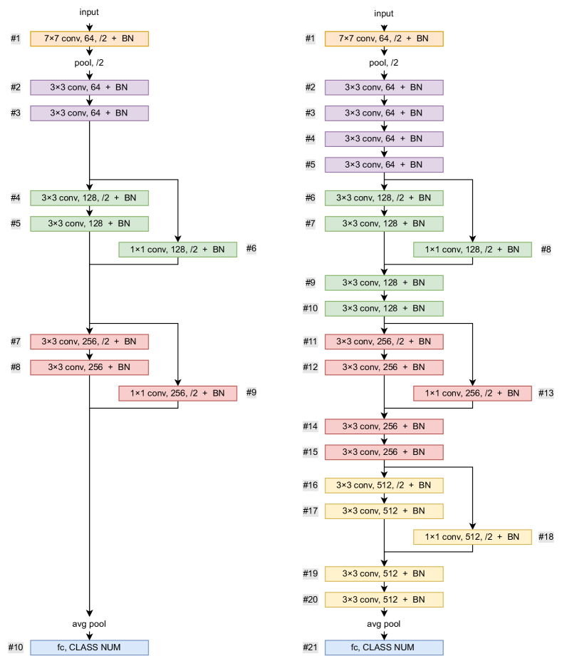
Figure 4: Model architecture and layer partitioning about our ResNet-8 and ResNet-18 model.

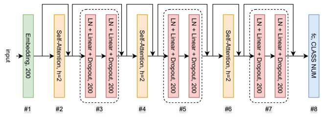
Figure 5: Model architecture and layer partitioning for language transformer.

Appendix B Proof for Convergence Rate of FedPart

Before beginning the proof, we need to analyze the upper bound of the gradient variance after parameter selection. According to Assumption 3, we know that for any mask matrices $S_{1},S_{2}$, it holds that:

$$\frac{\mathbb{E}_{x\sim\mathbf{D_{i}}}[||S_{1}\odot(\nabla\mathcal{L}(x|w)-\nabla f_{i}(w))||]}{\mathbb{E}_{x\sim\mathbf{D_{i}}}[||S_{2}\odot(\nabla\mathcal{L}(x|w)-\nabla f_{i}(w))||]}\leq k,\forall i,w,x\in\mathbf{D_{i}},S_{1},S_{2}$$ (10)

Constructively, we set a series of mask matrices $S_{1},\cdots,S_{M}$ that have no overlapping ’1’ elements at the same positions and their sum exactly forms an all-one matrix. Clearly, each of these mask matrices meets our requirements. Therefore, we can derive:

$$\mathbb{E}_{x\sim\mathbf{D_{i}}}[||S_{j}\odot(\nabla\mathcal{L}(x|w)-\nabla f_{i}(w))||^{2}]\geq\frac{1}{k^{2}}*{\mathbb{E}_{x\sim\mathbf{D_{i}}}[||S_{1}\odot(\nabla\mathcal{L}(x|w)-\nabla f_{i}(w))||^{2}]}$$ (11)

Summing over $j$ from 1 to $M$, the left-hand side of the inequality is exactly the variance of the gradient without any mask matrices. Therefore:

$$\sum_{j=1}^{M}\mathbb{E}_{x\sim\mathbf{D_{i}}}[||S_{j}\odot(\nabla\mathcal{L}(x|w)-\nabla f_{i}(w))||^{2}] =\mathbb{E}_{x\sim\mathbf{D_{i}}}[||\nabla\mathcal{L}(x|w)-\nabla f_{i}(w)||^{2}]$$

$$\geq\frac{M}{k^{2}}*{\mathbb{E}_{x\sim\mathbf{D_{i}}}[||S_{1}\odot(\nabla\mathcal{L}(x|w)-\nabla f_{i}(w))||^{2}]}$$

According to Assumption 2, the upper limit of the left side of the inequality is $\sigma^{2}$, so we finally obtain a general upper bound for the gradient with masks:

$$\mathbb{E}_{x\sim\mathbf{D_{i}}}[||S\odot(\nabla\mathcal{L}(x|w)-\nabla f_{i}(w))||^{2}]\leq\frac{\sigma^{2}k^{2}}{M},\forall i,w,x\in\mathbf{D_{i}},S$$ (12)

Having prepared the groundwork, we are now ready to begin the formal proof process. First, based on Assumption 1, as the loss function is L-smooth, we have:

$$\mathbb{E}[f(\bar{w}^{t})]\leq\mathbb{E}[f(\bar{w}^{t-1}]+\mathbb{E}[\left\langle S_{i}^{t}\odot\nabla f(\bar{w}^{t-1}),\bar{w}^{t}-\bar{w}^{t-1}\right\rangle]+\frac{L}{2}\mathbb{E}[||\bar{w}^{t}-\bar{w}^{t-1}||^{2}]$$ (13)

Next, we analyze the third term on the right-hand side of the inequality above to derive the following inequality:

$$\mathbb{E}[||\bar{w}^{t}-\bar{w}^{t-1}||^{2}] =\gamma^{2}\mathbb{E}[||\frac{1}{N}\sum_{i=1}^{N}S_{i}^{t}\odot G_{i}^{t}||^{2}]$$

$$=\gamma^{2}\mathbb{E}[||\frac{1}{N}\sum_{i=1}^{N}S_{i}^{t}\odot(G_{i}^{t}-\nabla f_{i}(w_{i}^{t-1}))||^{2}]+\gamma^{2}\mathbb{E}[||\frac{1}{N}\sum_{i=1}^{N}S_{i}^{t}\odot\nabla f_{i}(w_{i}^{t-1})||^{2}]$$

$$=\frac{\gamma^{2}}{N^{2}}\sum_{i=1}^{N}\mathbb{E}[||S_{i}^{t}\odot(G_{i}^{t}-\nabla f_{i}(w_{i}^{t-1}))||^{2}]+\gamma^{2}\mathbb{E}[||\frac{1}{N}\sum_{i=1}^{N}S_{i}^{t}\odot\nabla f_{i}(w_{i}^{t-1})||^{2}]$$

$$\leq\frac{\gamma^{2}\sigma^{2}k^{2}}{MN}+\gamma^{2}\mathbb{E}[||\frac{1}{N}\sum_{i=1}^{N}S_{i}^{t}\odot\nabla f_{i}(w_{i}^{t-1})||^{2}]$$

The last inequality comes from the derived Eq. 12. Next, we analyze the second term on the right-hand side of Eq. 13:

$$\mathbb{E}[\left\langle S_{i}^{t}\odot\nabla f(\bar{w}^{t-1}),\bar{w}^{t}-\bar{w}^{t-1}\right\rangle] =-\gamma\mathbb{E}[\left\langle S_{i}^{t}\odot\nabla f(\bar{w}^{t-1}),\frac{1}{N}\sum_{i=1}^{N}S_{i}^{t}\odot G_{i}^{t}\right\rangle]$$

$$=-\gamma\mathbb{E}[\left\langle S_{i}^{t}\odot\nabla f(\bar{w}^{t-1}),\frac{1}{N}\sum_{i=1}^{N}S_{i}^{t}\odot\nabla f_{i}(w_{i}^{t-1})\right\rangle]$$

$$=-\frac{\gamma}{2}\mathbb{E}[||S_{i}^{t}\odot\nabla f(\bar{w}^{t-1})||^{2}+||\frac{1}{N}\sum_{i=1}^{N}S_{i}^{t}\odot\nabla f_{i}(w_{i}^{t-1})||^{2}-$$

$$\quad\quad||S_{i}^{t}\odot\nabla f(\bar{w}^{t-1})-\frac{1}{N}\sum_{i=1}^{N}S_{i}^{t}\odot\nabla f_{i}(w_{i}^{t-1})||^{2}]$$

$$\leq-\frac{\gamma}{2}\mathbb{E}[||S_{i}^{t}\odot\nabla f(\bar{w}^{t-1})||^{2}+||\frac{1}{N}\sum_{i=1}^{N}S_{i}^{t}\odot\nabla f_{i}(w_{i}^{t-1})||^{2}-$$

$$\quad\quad||\nabla f(\bar{w}^{t-1})-\frac{1}{N}\sum_{i=1}^{N}\nabla f_{i}(w_{i}^{t-1})||^{2}]$$

Further expanding the right-hand side of the above inequality, we can obtain:

$$\mathbb{E}[||\nabla f(\bar{w}^{t-1})-\frac{1}{N}\sum_{i=1}^{N}\nabla f_{i}(w_{i}^{t-1})||^{2}] =\mathbb{E}[||\frac{1}{N}\sum_{i=1}^{N}\nabla f_{i}(\bar{w}^{t-1})-\frac{1}{N}\sum_{i=1}^{N}\nabla f_{i}(w_{i}^{t-1})||^{2}]$$

$$=\frac{1}{N^{2}}\mathbb{E}[||\sum_{i=1}^{N}(\nabla f_{i}(\bar{w}^{t-1})-\nabla f_{i}(w_{i}^{t-1}))||^{2}]$$

$$\leq\frac{1}{N}\mathbb{E}[\sum_{i=1}^{N}||\nabla f_{i}(\bar{w}^{t-1})-\nabla f_{i}(w_{i}^{t-1})||^{2}]$$

$$\leq\frac{L^{2}}{N}\sum_{i=1}^{N}\mathbb{E}[||\bar{w}^{t-1}-w_{i}^{t-1}||^{2}]$$

In the above derivation, we have used the assumption of L-smoothness and Jensen’s inequality. Next, we will continue to estimate the upper limit of this term. Assuming that the last time $t=t_{0}$ was a parameter aggregation, and the next time the parameters aggregate is at $t=t_{0}+E$, then:

$$\mathbb{E}[||\bar{w}^{t}-w_{i}^{t}||^{2}] =\mathbb{E}[||\gamma\sum_{\tau=t_{0}+1}^{t}\frac{1}{N}\sum_{i=1}^{N}S_{i}^{\tau}\odot G_{i}^{\tau}-\gamma\sum_{\tau=t_{0}+1}^{t}S_{i}^{\tau}\odot G_{i}^{\tau}||^{2}]$$

$$=\gamma^{2}\mathbb{E}[||\sum_{\tau=t_{0}+1}^{t}\frac{1}{N}\sum_{i=1}^{N}S_{i}^{\tau}\odot G_{i}^{\tau}-\sum_{\tau=t_{0}+1}^{t}S_{i}^{\tau}\odot G_{i}^{\tau}||^{2}]$$

$$\leq 2\gamma^{2}\mathbb{E}[||\sum_{\tau=t_{0}+1}^{t}\frac{1}{N}\sum_{i=1}^{N}S_{i}^{\tau}\odot G_{i}^{\tau}||^{2}+||\sum_{\tau=t_{0}+1}^{t}S_{i}^{\tau}\odot G_{i}^{\tau}||^{2}]$$

$$\leq 2(t-t_{0})\gamma^{2}\mathbb{E}[\sum_{\tau=t_{0}+1}^{t}||\frac{1}{N}\sum_{i=1}^{N}S_{i}^{\tau}\odot G_{i}^{\tau}||^{2}+\sum_{\tau=t_{0}+1}^{t}||S_{i}^{\tau}\odot G_{i}^{\tau}||^{2}]$$

$$\leq 2(t-t_{0})\gamma^{2}\mathbb{E}[\sum_{\tau=t_{0}+1}^{t}\sum_{i=1}^{N}\frac{1}{N}||S_{i}^{\tau}\odot G_{i}^{\tau}||^{2}+\sum_{\tau=t_{0}+1}^{t}||S_{i}^{\tau}\odot G_{i}^{\tau}||^{2}]$$

$$\leq 4(t-t_{0})\gamma^{2}G^{2}\leq 4E\gamma^{2}G^{2}$$

Substituting all the above inequalities into the right side of Eq. 13, we can finally obtain that when using a learning rate $0\leq\gamma\leq\frac{1}{L}$, it satisfies:

$$\mathbb{E}[f(\bar{w}^{t})] \leq\mathbb{E}[f(\bar{w}^{t-1})]-\frac{\gamma-\gamma^{2}L}{2}\mathbb{E}[||\frac{1}{N}\sum_{i=1}^{N}S_{i}^{t}\odot\nabla f_{i}(w_{i}^{t-1})||^{2}$$

$$\quad\quad-\frac{\gamma}{2}\mathbb{E}[||S_{i}^{t}\odot\nabla f(\bar{w}^{t-1})||^{2}+2\gamma^{3}E^{2}G^{2}L^{2}+\frac{L}{2NM}\gamma^{2}\sigma^{2}k^{2}$$

$$\leq\mathbb{E}[f(\bar{w}^{t-1})]-\frac{\gamma}{2}\mathbb{E}[||S_{i}^{t}\odot\nabla f(\bar{w}^{t-1})||^{2}+2\gamma^{3}E^{2}G^{2}L^{2}+\frac{L}{2NM}\gamma^{2}\sigma^{2}k^{2}$$

After rearranging the above inequalities, we obtain

$$\mathbb{E}[||S_{i}^{t}\odot\nabla f(\bar{w}^{t-1})||^{2}\leq\frac{2}{\gamma}(\mathbb{E}[f(\bar{w}^{t-1})]-\mathbb{E}[f(\bar{w}^{t})])+4\gamma^{2}E^{2}G^{2}L^{2}+\frac{L}{NM}\gamma\sigma^{2}k^{2}$$ (14)

Finally, summing the inequalities from $t=1,\cdots,T$, and multiplying both sides by $\frac{1}{T}$, we can obtain:

$$\frac{1}{T}\sum_{i=1}^{T}\mathbb{E}[||S_{i}^{t}\odot\nabla f(\bar{w}^{t-1})||^{2}\leq\frac{2}{\gamma T}(f(\bar{w}^{0})-f^{*})+4\gamma^{2}E^{2}G^{2}L^{2}+\frac{L}{NM}\gamma\sigma^{2}k^{2}$$ (15)

Selecting a learning rate $\gamma=\frac{\sqrt{NM}}{L\sqrt{T}}$, we can obtain: $\frac{1}{T}\sum_{i=1}^{T}\mathbb{E}[||S_{i}^{t}\odot\nabla f(\bar{w}^{t-1})||^{2}\leq\frac{2L}{\sqrt{NMT}}(f(\bar{w}^{0})-f^{*})+\frac{4NME^{2}G^{2}}{T}+\frac{\sigma^{2}k^{2}}{\sqrt{NMT}}$. Further choosing $E\leq\frac{T^{1/4}}{(MN)^{3/4}}$, we can obtain a further corollary: $\frac{1}{T}\sum_{i=1}^{T}\mathbb{E}[||S_{i}^{t}\odot\nabla f(\bar{w}^{t-1})||^{2}\leq\frac{2L}{\sqrt{NMT}}(f(\bar{w}^{0})-f^{*})+\frac{4G^{2}}{\sqrt{MNT}}+\frac{\sigma^{2}k^{2}}{\sqrt{NMT}}=O(\frac{1}{\sqrt{NMT}})$. This proves the convergence rate of FedPart.

Appendix C Visualizations for Activation Maximization

For better visualizing the semantic information recognized by each layer in the different models, in Fig. 6, we present representative results from the first and last layers of models under four scenarios: FedAvg-100, FedPart(No Init. 1C), FedPart(1C), and FedPart(5C).

From the visualization results, it can be observed that FedAvg-100, due to being a full network update, captures low-level semantic features (such as clear boundaries) in shallow layers, while deeper layers capture complex semantic information. However, the results of FedPart(No Init. 1C) exhibit noticeable differences in color and structural features compared to the full network update. This verifies our conjunction that partial network update is detrimental to forming such a hierarchical information extraction approach, leading to the model converging to possible local minima. Additionally, we can also see that by including the initial phase of full network updates and multiple rounds of sequential training, the similarity of semantic information obtained by the model gradually approaches that of FedAvg. Therefore, the results sufficiently demonstrate that although we only train one layer of the network each time, by employing an appropriate layer selection scheme, we ultimately achieve an effect close to that of full network updates.

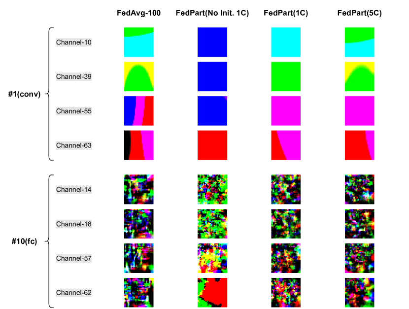
Figure 6: Activation maximization images of different channels within different layers.

Appendix D Visualizations for Convolutional Kernel

To visually depict the characteristics of the convolutional kernels in the first convolutional layer of different models, we conduct kernel visualization. The four models we select come from the following scenarios: FedAvg-100, FedPart(No Init. 1C), FedPart(1C), and FedPart(5C).

In Fig. 7, we present a comparison of results for planes in the first convolutional layer. It can be seen that the kernels in the first convolutional layer of the FedAvg-100 model are mostly edge and corner detectors. In contrast, the results of FedPart(No Init. 1C) and FedPart(1C) appear more random and irregular. However, after training to convergence, the results of FedPart(5C) are noticeably more similar to those of FedAvg-100, and start to exhibit characteristics of simple feature extractors. This indicates that through partial network updates, the layers of the model gradually coordinate with each other, yielding a cooperative effect.

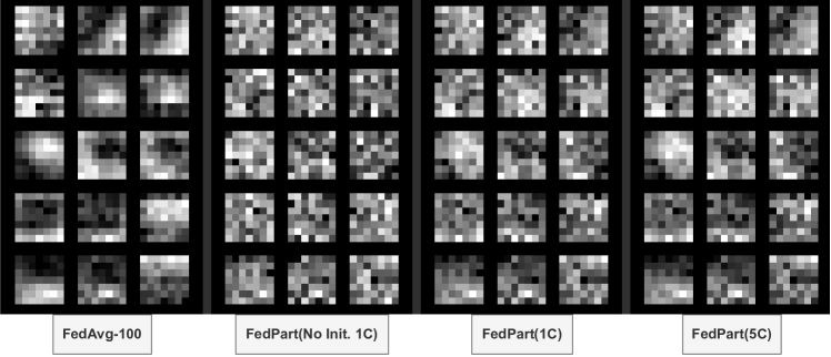
Figure 7: Convolutional kernel visualization results of 5 planes in the first convolutional layer. Each plane include three color channels of image.

Appendix E Robustness to Privacy Attack

In this section, we will provide a detailed introduction to the results of privacy leakage using the DLG method on full network updates and partial network updates. We perform DLG attacks in four settings: transmiting all parameters in FedAvg-100 model; and transmiting only the parameters of layers $\#1$, $\#9$, and $\#10$ separately in FedPart(5C) model. In Fig. 8, we select some representative reconstructed images. The leftmost column represents the original images, while the four columns on the right show the reconstructed images obtained through DLG attacks under different settings.

It can be observed that in the FedAvg-100 scenario, the reconstructed images have the highest quality, exhibiting significant similarity to the original images. However, when adopting partial network updates, the reconstruction quality is poor. Apart from minor color correlations, the reconstructed images exhibit significant differences in structural features compared to the originals. This validates our claim that under the FedPart method, transmitting only a subset of parameters can effectively preserve data privacy.

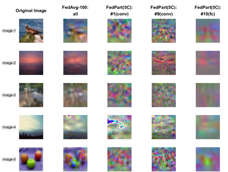
Figure 8: The reconstructed images from DLG attacks on full network of FedAvg-100 and different partial network of FedPart(5C).

Appendix F Additional Experiments

F.1 Learning Rate Tuning

In this section, we explore the appropriate learning rate for our experimental configurations. We conduct experiments on the CIFAR-100 dataset using ResNet-8 for both FNU and PNU methods. The experimental results for Adam optimizer with different learning rates are shown in Table 10.

From the results, it can be seen that both FNU and PNU methods perform best with a learning rate of 0.001. So in our experimental configurations, the Adam optimizer with a learning rate of 0.001 is finally chosen.

Table 10: Performances (Best Acc.) for different learning rate in full network and partial network updates.

Dataset	Cycle	FedAvg-FNU			FedPart
		lr=0.0001	lr=0.001	lr=0.01	lr=0.0001	lr=0.001	lr=0.01
CIFAR- 100	1	24.82	30.68	28.15	16.56	31.36	23.41
	2	30.08	32.53	30.13	21.88	34.70	30.10
	3	31.91	34.02	30.93	25.42	36.34	31.94
	4	32.45	35.91	30.93	27.85	37.12	32.54
	5	32.95	35.91	31.65	29.98	37.70	33.31

F.2 Evaluation of Client Sampling

In this section, we conduct experiments with 150 clients, randomly sampling 20% of the clients for training and aggregation in each communication round. The experimental results are shown in Table 11. Our method achieves final performance improvements of +2.1%, +1.6%, and +3.4% on CIFAR-10, CIFAR-100, and Tiny-ImageNet, respectively, indicating that FedPart performs better than FedAvg in this scenario.

Table 11: Performance of FedPart with client sampling.

Dataset	C	FedAvg-FNU	FedPart
CIFAR- 10	2	60.82	63.22
	3	61.50	63.22
	4	64.34	66.08
	5	65.00	67.08
CIFAR- 100	2	34.82	37.13
	3	39,36	37.13
	4	39.64	41.00
	5	40.55	42.12
Tiny- ImageNet	2	19.63	23.06
	3	19.63	23.06
	4	22.01	26.03
	5	23.33	26.75

F.3 Analysis under Extreme Data Heterogeneity

In this section, we conduct experiments with an $\alpha=0.1$ setting as data heterogeneity is more severe. The experimental results are shown in Table 12.

It can be seen that, in this extreme non-IID scenario ($\alpha=0.1$), the model accuracy of our method is roughly on par with that of the full parameter method. However, this does not imply that FedPart offers no performance advantages—the benefits primarily arise from reduced communication and computation costs. The results indicate that FedPart can achieve similar accuracy to FedAvg while significantly reducing communication and computation costs (these metrics are consistent with those observed in the IID scenario). As shown in Table 1, when training on Tiny-ImageNet, FedPart reduces communication overhead by 72% and computation overhead by 27%. Therefore, we believe that even in such an extreme scenario of data heterogeneity, our method still holds practical value.

Table 12: Performance of FL algorithms with full network and partial network updates under extreme data heterogeneity (Dirichlet, $\alpha=0.1$)

Data	C	FedAvg		FedProx
		FNU	FedPart	FNU	FedPart
CIFAR- 10	1	33.79	44.02	39.64	43.85
	2	44.08	44.41	46.88	45.42

Appendix G Justification of Assumption 3

In Assumption 3 in Section 3.3, we assume that for any mask matrices $S_{1},S_{2}$, it holds that:

$$\frac{\mathbb{E}_{x\sim\mathbf{D_{i}}}[||S_{1}\odot(\nabla\mathcal{L}(x|w)-\nabla f_{i}(w))||]}{\mathbb{E}_{x\sim\mathbf{D_{i}}}[||S_{2}\odot(\nabla\mathcal{L}(x|w)-\nabla f_{i}(w))||]}\leq k,\forall i,w,x\in\mathbf{D_{i}},S_{1},S_{2}$$ (16)

Regarding the value of $k$ on the right side of the equation above, recall Eq. 15 in Appendix B, the convergence rate of FedPart satisfies:

$$\frac{1}{T}\sum_{i=1}^{T}\mathbb{E}[||S_{i}^{t}\odot\nabla f(\bar{w}^{t-1})||^{2}\leq\frac{2}{\gamma T}(f(\bar{w}^{0})-f^{*})+4\gamma^{2}E^{2}G^{2}L^{2}+\frac{L}{NM}\gamma\sigma^{2}k^{2}$$

Therefore, theoretically, the smaller the value of $k$, the smaller the value on the right side of this inequality, leading to improved convergence of FedPart. Hence, it is important to carefully examine the value range of $k$ in practice.

We begin with analysing the lower bound of $k$. Since $S_{1}$ and $S_{2}$ are arbitrary, it possible that $S_{1}=S_{2}$, indicating a lower bound of 1 for the value $k$. As for approximating the upper bound of the $k$, we conduct Monte Carlo simulations on real-world nueral networks.

We test the $k$ values in three neural networks at different training stages. For each neural networks, we conduct Monte Carlo simulations for 10,000 samples to accurately approximate the value of $k$. The experimental results are shown in Table 13. We can see that $k$ is close to 1 under different settings, which proves that the effect of applying different masks to the variability of gradient is similar, thus strongly supporting Assumption 3.

Table 13: Monte Carlo simulation experiments for the value of $k$.

	ResNet-8	ResNet-18
0% Training (Random initialized)	1.09	1.08
50% Training (Intermediate)	1.13	1.18
100% Training (Fully trained)	1.13	1.17

NeurIPS Paper Checklist

1. Claims

2. Question: Do the main claims made in the abstract and introduction accurately reflect the paper’s contributions and scope?

3. Answer: [Yes]

4. Justification: The following content of this paper is centered on the partial network updating method introduced in the abstract and introduction.

5. Guidelines:

   • The answer NA means that the abstract and introduction do not include the claims made in the paper.

   • The abstract and/or introduction should clearly state the claims made, including the contributions made in the paper and important assumptions and limitations. A No or NA answer to this question will not be perceived well by the reviewers.

   • The claims made should match theoretical and experimental results, and reflect how much the results can be expected to generalize to other settings.

   • It is fine to include aspirational goals as motivation as long as it is clear that these goals are not attained by the paper.

6. Limitations

7. Question: Does the paper discuss the limitations of the work performed by the authors?

8. Answer: [Yes]

9. Justification: We have discussed our limitations in the conclusion section.

10. Guidelines:

    • The answer NA means that the paper has no limitation while the answer No means that the paper has limitations, but those are not discussed in the paper.

    • The authors are encouraged to create a separate "Limitations" section in their paper.

    • The paper should point out any strong assumptions and how robust the results are to violations of these assumptions (e.g., independence assumptions, noiseless settings, model well-specification, asymptotic approximations only holding locally). The authors should reflect on how these assumptions might be violated in practice and what the implications would be.

    • The authors should reflect on the scope of the claims made, e.g., if the approach was only tested on a few datasets or with a few runs. In general, empirical results often depend on implicit assumptions, which should be articulated.

    • The authors should reflect on the factors that influence the performance of the approach. For example, a facial recognition algorithm may perform poorly when image resolution is low or images are taken in low lighting. Or a speech-to-text system might not be used reliably to provide closed captions for online lectures because it fails to handle technical jargon.

    • The authors should discuss the computational efficiency of the proposed algorithms and how they scale with dataset size.

    • If applicable, the authors should discuss possible limitations of their approach to address problems of privacy and fairness.

    • While the authors might fear that complete honesty about limitations might be used by reviewers as grounds for rejection, a worse outcome might be that reviewers discover limitations that aren’t acknowledged in the paper. The authors should use their best judgment and recognize that individual actions in favor of transparency play an important role in developing norms that preserve the integrity of the community. Reviewers will be specifically instructed to not penalize honesty concerning limitations.

11. Theory Assumptions and Proofs

12. Question: For each theoretical result, does the paper provide the full set of assumptions and a complete (and correct) proof?

13. Answer: [Yes]

14. Justification: The full set of assumptions is provided in Section 3.3, and a complete proof is available in Appendix B.

15. Guidelines:

    • The answer NA means that the paper does not include theoretical results.

    • All the theorems, formulas, and proofs in the paper should be numbered and cross-referenced.

    • All assumptions should be clearly stated or referenced in the statement of any theorems.

    • The proofs can either appear in the main paper or the supplemental material, but if they appear in the supplemental material, the authors are encouraged to provide a short proof sketch to provide intuition.

    • Inversely, any informal proof provided in the core of the paper should be complemented by formal proofs provided in appendix or supplemental material.

    • Theorems and Lemmas that the proof relies upon should be properly referenced.

16. Experimental Result Reproducibility

17. Question: Does the paper fully disclose all the information needed to reproduce the main experimental results of the paper to the extent that it affects the main claims and/or conclusions of the paper (regardless of whether the code and data are provided or not)?

18. Answer: [Yes]

19. Justification: We release our complete code in the supplementary materials.

20. Guidelines:

    • The answer NA means that the paper does not include experiments.

    • If the paper includes experiments, a No answer to this question will not be perceived well by the reviewers: Making the paper reproducible is important, regardless of whether the code and data are provided or not.

    • If the contribution is a dataset and/or model, the authors should describe the steps taken to make their results reproducible or verifiable.

    • Depending on the contribution, reproducibility can be accomplished in various ways. For example, if the contribution is a novel architecture, describing the architecture fully might suffice, or if the contribution is a specific model and empirical evaluation, it may be necessary to either make it possible for others to replicate the model with the same dataset, or provide access to the model. In general. releasing code and data is often one good way to accomplish this, but reproducibility can also be provided via detailed instructions for how to replicate the results, access to a hosted model (e.g., in the case of a large language model), releasing of a model checkpoint, or other means that are appropriate to the research performed.

    • While NeurIPS does not require releasing code, the conference does require all submissions to provide some reasonable avenue for reproducibility, which may depend on the nature of the contribution. For example

      1. If the contribution is primarily a new algorithm, the paper should make it clear how to reproduce that algorithm.

      2. If the contribution is primarily a new model architecture, the paper should describe the architecture clearly and fully.

      3. If the contribution is a new model (e.g., a large language model), then there should either be a way to access this model for reproducing the results or a way to reproduce the model (e.g., with an open-source dataset or instructions for how to construct the dataset).

      4. We recognize that reproducibility may be tricky in some cases, in which case authors are welcome to describe the particular way they provide for reproducibility. In the case of closed-source models, it may be that access to the model is limited in some way (e.g., to registered users), but it should be possible for other researchers to have some path to reproducing or verifying the results.

21. Open access to data and code

22. Question: Does the paper provide open access to the data and code, with sufficient instructions to faithfully reproduce the main experimental results, as described in supplemental material?

23. Answer: [Yes]

24. Justification: This full code is released in the supplementary materials, and the datasets are also public.

25. Guidelines:

    • The answer NA means that paper does not include experiments requiring code.

    • Please see the NeurIPS code and data submission guidelines (https://nips.cc/public/guides/CodeSubmissionPolicy) for more details.

    • While we encourage the release of code and data, we understand that this might not be possible, so “No” is an acceptable answer. Papers cannot be rejected simply for not including code, unless this is central to the contribution (e.g., for a new open-source benchmark).

    • The instructions should contain the exact command and environment needed to run to reproduce the results. See the NeurIPS code and data submission guidelines (https://nips.cc/public/guides/CodeSubmissionPolicy) for more details.

    • The authors should provide instructions on data access and preparation, including how to access the raw data, preprocessed data, intermediate data, and generated data, etc.

    • The authors should provide scripts to reproduce all experimental results for the new proposed method and baselines. If only a subset of experiments are reproducible, they should state which ones are omitted from the script and why.

    • At submission time, to preserve anonymity, the authors should release anonymized versions (if applicable).

    • Providing as much information as possible in supplemental material (appended to the paper) is recommended, but including URLs to data and code is permitted.

26. Experimental Setting/Details

27. Question: Does the paper specify all the training and test details (e.g., data splits, hyperparameters, how they were chosen, type of optimizer, etc.) necessary to understand the results?

28. Answer: [Yes]

29. Justification: We state important details in our main paper, while the full information can be viewed in our released code.

30. Guidelines:

    • The answer NA means that the paper does not include experiments.

    • The experimental setting should be presented in the core of the paper to a level of detail that is necessary to appreciate the results and make sense of them.

    • The full details can be provided either with the code, in appendix, or as supplemental material.

31. Experiment Statistical Significance

32. Question: Does the paper report error bars suitably and correctly defined or other appropriate information about the statistical significance of the experiments?

33. Answer: [Yes]

34. Justification: The main results in our paper is repeated for 3 different random seeds and we have shown the error bar for each metric.

35. Guidelines:

    • The answer NA means that the paper does not include experiments.

    • The authors should answer "Yes" if the results are accompanied by error bars, confidence intervals, or statistical significance tests, at least for the experiments that support the main claims of the paper.

    • The factors of variability that the error bars are capturing should be clearly stated (for example, train/test split, initialization, random drawing of some parameter, or overall run with given experimental conditions).

    • The method for calculating the error bars should be explained (closed form formula, call to a library function, bootstrap, etc.)

    • The assumptions made should be given (e.g., Normally distributed errors).

    • It should be clear whether the error bar is the standard deviation or the standard error of the mean.

    • It is OK to report 1-sigma error bars, but one should state it. The authors should preferably report a 2-sigma error bar than state that they have a 96% CI, if the hypothesis of Normality of errors is not verified.

    • For asymmetric distributions, the authors should be careful not to show in tables or figures symmetric error bars that would yield results that are out of range (e.g. negative error rates).

    • If error bars are reported in tables or plots, The authors should explain in the text how they were calculated and reference the corresponding figures or tables in the text.

36. Experiments Compute Resources

37. Question: For each experiment, does the paper provide sufficient information on the computer resources (type of compute workers, memory, time of execution) needed to reproduce the experiments?

38. Answer: [Yes]

39. Justification: Descriptions about the resources required is stated in Section 4.

40. Guidelines:

    • The answer NA means that the paper does not include experiments.

    • The paper should indicate the type of compute workers CPU or GPU, internal cluster, or cloud provider, including relevant memory and storage.

    • The paper should provide the amount of compute required for each of the individual experimental runs as well as estimate the total compute.

    • The paper should disclose whether the full research project required more compute than the experiments reported in the paper (e.g., preliminary or failed experiments that didn’t make it into the paper).

41. Code Of Ethics

42. Question: Does the research conducted in the paper conform, in every respect, with the NeurIPS Code of Ethics https://neurips.cc/public/EthicsGuidelines?

43. Answer: [Yes]

44. Justification: The research conducted in the paper conform, in every respect, with the NeurIPS Code of Ethics.

45. Guidelines:

    • The answer NA means that the authors have not reviewed the NeurIPS Code of Ethics.

    • If the authors answer No, they should explain the special circumstances that require a deviation from the Code of Ethics.

    • The authors should make sure to preserve anonymity (e.g., if there is a special consideration due to laws or regulations in their jurisdiction).

46. Broader Impacts

47. Question: Does the paper discuss both potential positive societal impacts and negative societal impacts of the work performed?

48. Answer: [Yes]

49. Justification: This paper may have positive societal impacts due to its better ability for privacy protection, which is discussed in Section 4

50. Guidelines:

    • The answer NA means that there is no societal impact of the work performed.

    • If the authors answer NA or No, they should explain why their work has no societal impact or why the paper does not address societal impact.

    • Examples of negative societal impacts include potential malicious or unintended uses (e.g., disinformation, generating fake profiles, surveillance), fairness considerations (e.g., deployment of technologies that could make decisions that unfairly impact specific groups), privacy considerations, and security considerations.

    • The conference expects that many papers will be foundational research and not tied to particular applications, let alone deployments. However, if there is a direct path to any negative applications, the authors should point it out. For example, it is legitimate to point out that an improvement in the quality of generative models could be used to generate deepfakes for disinformation. On the other hand, it is not needed to point out that a generic algorithm for optimizing neural networks could enable people to train models that generate Deepfakes faster.

    • The authors should consider possible harms that could arise when the technology is being used as intended and functioning correctly, harms that could arise when the technology is being used as intended but gives incorrect results, and harms following from (intentional or unintentional) misuse of the technology.

    • If there are negative societal impacts, the authors could also discuss possible mitigation strategies (e.g., gated release of models, providing defenses in addition to attacks, mechanisms for monitoring misuse, mechanisms to monitor how a system learns from feedback over time, improving the efficiency and accessibility of ML).

51. Safeguards

52. Question: Does the paper describe safeguards that have been put in place for responsible release of data or models that have a high risk for misuse (e.g., pretrained language models, image generators, or scraped datasets)?

53. Answer: [N/A]

54. Justification: This paper poses no such risks.

55. Guidelines:

    • The answer NA means that the paper poses no such risks.

    • Released models that have a high risk for misuse or dual-use should be released with necessary safeguards to allow for controlled use of the model, for example by requiring that users adhere to usage guidelines or restrictions to access the model or implementing safety filters.

    • Datasets that have been scraped from the Internet could pose safety risks. The authors should describe how they avoided releasing unsafe images.

    • We recognize that providing effective safeguards is challenging, and many papers do not require this, but we encourage authors to take this into account and make a best faith effort.

56. Licenses for existing assets

57. Question: Are the creators or original owners of assets (e.g., code, data, models), used in the paper, properly credited and are the license and terms of use explicitly mentioned and properly respected?

58. Answer: [Yes]

59. Justification: Owners of the assets used in this paper is properly credited.

60. Guidelines:

    • The answer NA means that the paper does not use existing assets.

    • The authors should cite the original paper that produced the code package or dataset.

    • The authors should state which version of the asset is used and, if possible, include a URL.

    • The name of the license (e.g., CC-BY 4.0) should be included for each asset.

    • For scraped data from a particular source (e.g., website), the copyright and terms of service of that source should be provided.

    • If assets are released, the license, copyright information, and terms of use in the package should be provided. For popular datasets, paperswithcode.com/datasets has curated licenses for some datasets. Their licensing guide can help determine the license of a dataset.

    • For existing datasets that are re-packaged, both the original license and the license of the derived asset (if it has changed) should be provided.

    • If this information is not available online, the authors are encouraged to reach out to the asset’s creators.

61. New Assets

62. Question: Are new assets introduced in the paper well documented and is the documentation provided alongside the assets?

63. Answer: [Yes]

64. Justification: The code for this paper is well documented and is provided in the supplimentary material.

65. Guidelines:

    • The answer NA means that the paper does not release new assets.

    • Researchers should communicate the details of the dataset/code/model as part of their submissions via structured templates. This includes details about training, license, limitations, etc.

    • The paper should discuss whether and how consent was obtained from people whose asset is used.

    • At submission time, remember to anonymize your assets (if applicable). You can either create an anonymized URL or include an anonymized zip file.

66. Crowdsourcing and Research with Human Subjects

67. Question: For crowdsourcing experiments and research with human subjects, does the paper include the full text of instructions given to participants and screenshots, if applicable, as well as details about compensation (if any)?

68. Answer: [N/A]

69. Justification: This paper does not involve crowdsourcing nor research with human subjects.

70. Guidelines:

    • The answer NA means that the paper does not involve crowdsourcing nor research with human subjects.

    • Including this information in the supplemental material is fine, but if the main contribution of the paper involves human subjects, then as much detail as possible should be included in the main paper.

    • According to the NeurIPS Code of Ethics, workers involved in data collection, curation, or other labor should be paid at least the minimum wage in the country of the data collector.

71. Institutional Review Board (IRB) Approvals or Equivalent for Research with Human Subjects

72. Question: Does the paper describe potential risks incurred by study participants, whether such risks were disclosed to the subjects, and whether Institutional Review Board (IRB) approvals (or an equivalent approval/review based on the requirements of your country or institution) were obtained?

73. Answer: [N/A]

74. Justification: This paper poses no such risks.

75. Guidelines:

    • The answer NA means that the paper does not involve crowdsourcing nor research with human subjects.

    • Depending on the country in which research is conducted, IRB approval (or equivalent) may be required for any human subjects research. If you obtained IRB approval, you should clearly state this in the paper.

    • We recognize that the procedures for this may vary significantly between institutions and locations, and we expect authors to adhere to the NeurIPS Code of Ethics and the guidelines for their institution.

    • For initial submissions, do not include any information that would break anonymity (if applicable), such as the institution conducting the review.

References

- Abreha et al. (2022) H. G. Abreha, M. Hayajneh, and M. A. Serhani. Federated learning in edge computing: a systematic survey. Sensors, 22(2):450, 2022.
- Alam et al. (2022) S. Alam, L. Liu, M. Yan, and M. Zhang. Fedrolex: Model-heterogeneous federated learning with rolling sub-model extraction. Advances in neural information processing systems, 35:29677–29690, 2022.
- Alistarh et al. (2017) D. Alistarh, D. Grubic, J. Li, R. Tomioka, and M. Vojnovic. Qsgd: Communication-efficient sgd via gradient quantization and encoding. Advances in neural information processing systems, 30, 2017.
- Arivazhagan et al. (2019) M. G. Arivazhagan, V. Aggarwal, A. K. Singh, and S. Choudhary. Federated learning with personalization layers. arXiv preprint arXiv:1912.00818, 2019.
- Caldas et al. (2018) S. Caldas, J. Konečny, H. B. McMahan, and A. Talwalkar. Expanding the reach of federated learning by reducing client resource requirements. arXiv preprint arXiv:1812.07210, 2018.
- Chen et al. (2022) D. Chen, D. Gao, W. Kuang, Y. Li, and B. Ding. pfl-bench: A comprehensive benchmark for personalized federated learning. Advances in Neural Information Processing Systems, 35:9344–9360, 2022.
- Chen and Chao (2021) H.-Y. Chen and W.-L. Chao. On bridging generic and personalized federated learning for image classification. arXiv preprint arXiv:2107.00778, 2021.
- Diao et al. (2020) E. Diao, J. Ding, and V. Tarokh. Heterofl: Computation and communication efficient federated learning for heterogeneous clients. arXiv preprint arXiv:2010.01264, 2020.
- Erhan et al. (2009) D. Erhan, Y. Bengio, A. Courville, and P. Vincent. Visualizing higher-layer features of a deep network. University of Montreal, 1341(3):1, 2009.
- Ghadimi and Lan (2013) S. Ghadimi and G. Lan. Stochastic first-and zeroth-order methods for nonconvex stochastic programming. SIAM journal on optimization, 23(4):2341–2368, 2013.
- Hard et al. (2018) A. S. Hard, K. Rao, R. Mathews, F. Beaufays, S. Augenstein, H. Eichner, C. Kiddon, and D. Ramage. Federated learning for mobile keyboard prediction. ArXiv, abs/1811.03604, 2018.
- He et al. (2016) K. He, X. Zhang, S. Ren, and J. Sun. Deep residual learning for image recognition. In Proceedings of the IEEE conference on computer vision and pattern recognition, pages 770–778, 2016.
- Hobbhahn and Sevilla (2021) M. Hobbhahn and J. Sevilla. What’s the backward-forward flop ratio for neural networks?, 2021. URL https://epochai.org/blog/backward-forward-FLOP-ratio. Accessed: 2024-04-22.
- Hore and Ziou (2010) A. Hore and D. Ziou. Image quality metrics: Psnr vs. ssim. In 2010 20th international conference on pattern recognition, pages 2366–2369. IEEE, 2010.
- Horvath et al. (2021) S. Horvath, S. Laskaridis, M. Almeida, I. Leontiadis, S. Venieris, and N. Lane. Fjord: Fair and accurate federated learning under heterogeneous targets with ordered dropout. Advances in Neural Information Processing Systems, 34:12876–12889, 2021.
- Kairouz et al. (2019) P. Kairouz, H. B. McMahan, B. Avent, A. Bellet, M. Bennis, A. N. Bhagoji, K. Bonawitz, Z. B. Charles, G. Cormode, R. Cummings, R. G. L. D’Oliveira, S. Y. E. Rouayheb, D. Evans, J. Gardner, Z. Garrett, A. Gascón, B. Ghazi, P. B. Gibbons, M. Gruteser, Z. Harchaoui, C. He, L. He, Z. Huo, B. Hutchinson, J. Hsu, M. Jaggi, T. Javidi, G. Joshi, M. Khodak, J. Konecný, A. Korolova, F. Koushanfar, O. Koyejo, T. Lepoint, Y. Liu, P. Mittal, M. Mohri, R. Nock, A. Özgür, R. Pagh, M. Raykova, H. Qi, D. Ramage, R. Raskar, D. X. Song, W. Song, S. U. Stich, Z. Sun, A. T. Suresh, F. Tramèr, P. Vepakomma, J. Wang, L. Xiong, Z. Xu, Q. Yang, F. X. Yu, H. Yu, and S. Zhao. Advances and open problems in federated learning. Found. Trends Mach. Learn., 14:1–210, 2019.
- Karimireddy et al. (2020) S. P. Karimireddy, S. Kale, M. Mohri, S. Reddi, S. Stich, and A. T. Suresh. SCAFFOLD: Stochastic controlled averaging for federated learning. In H. D. III and A. Singh, editors, Proceedings of the 37th International Conference on Machine Learning, volume 119 of Proceedings of Machine Learning Research, pages 5132–5143. PMLR, 13–18 Jul 2020. URL https://proceedings.mlr.press/v119/karimireddy20a.html.
- Kingma and Ba (2014) D. P. Kingma and J. Ba. Adam: A method for stochastic optimization. arXiv preprint arXiv:1412.6980, 2014.
- Krizhevsky et al. (2009) A. Krizhevsky, G. Hinton, et al. Learning multiple layers of features from tiny images. 2009.
- Krizhevsky et al. (2010) A. Krizhevsky, V. Nair, and G. Hinton. Cifar-10 (canadian institute for advanced research), 2010.
- Le and Yang (2015) Y. Le and X. Yang. Tiny imagenet visual recognition challenge. CS 231N, 7(7):3, 2015.
- Li et al. (2021a) Q. Li, B. He, and D. X. Song. Model-contrastive federated learning. 2021 IEEE/CVF Conference on Computer Vision and Pattern Recognition (CVPR), pages 10708–10717, 2021a.
- Li et al. (2019) T. Li, A. K. Sahu, A. Talwalkar, and V. Smith. Federated learning: Challenges, methods, and future directions. IEEE Signal Processing Magazine, 37:50–60, 2019.
- Li et al. (2021b) X. Li, M. Jiang, X. Zhang, M. Kamp, and Q. Dou. Fedbn: Federated learning on non-iid features via local batch normalization. arXiv preprint arXiv:2102.07623, 2021b.
- Lian et al. (2017) X. Lian, C. Zhang, H. Zhang, C.-J. Hsieh, W. Zhang, and J. Liu. Can decentralized algorithms outperform centralized algorithms? a case study for decentralized parallel stochastic gradient descent. Advances in neural information processing systems, 30, 2017.
- McMahan et al. (2017) B. McMahan, E. Moore, D. Ramage, S. Hampson, and B. A. y Arcas. Communication-efficient learning of deep networks from decentralized data. In Artificial intelligence and statistics, pages 1273–1282. PMLR, 2017.
- Pfeiffer et al. (2022) K. Pfeiffer, M. Rapp, R. Khalili, and J. Henkel. Cocofl: Communication-and computation-aware federated learning via partial nn freezing and quantization. arXiv preprint arXiv:2203.05468, 2022.
- (28) B. Poczos and R. Tibshirani. Coordinate descent. https://www.stat.cmu.edu/~ryantibs/convexopt-F13/lectures/24-coord-desc.pdf. [Online; accessed March 31, 2024].
- Raghu et al. (2017) M. Raghu, J. Gilmer, J. Yosinski, and J. Sohl-Dickstein. Svcca: Singular vector canonical correlation analysis for deep learning dynamics and interpretability. Advances in neural information processing systems, 30, 2017.
- Rasley et al. (2020) J. Rasley, S. Rajbhandari, O. Ruwase, and Y. He. Deepspeed: System optimizations enable training deep learning models with over 100 billion parameters. Proceedings of the 26th ACM SIGKDD International Conference on Knowledge Discovery & Data Mining, 2020. URL https://api.semanticscholar.org/CorpusID:221191193.
- Rieke et al. (2020) N. Rieke, J. Hancox, W. Li, F. Milletarì, H. R. Roth, S. Albarqouni, S. Bakas, M. Galtier, B. A. Landman, K. H. Maier-Hein, S. Ourselin, M. J. Sheller, R. M. Summers, A. Trask, D. Xu, M. Baust, and M. J. Cardoso. The future of digital health with federated learning. NPJ Digital Medicine, 3, 2020.
- Rusu et al. (2016) A. A. Rusu, N. C. Rabinowitz, G. Desjardins, H. Soyer, J. Kirkpatrick, K. Kavukcuoglu, R. Pascanu, and R. Hadsell. Progressive neural networks. arXiv preprint arXiv:1606.04671, 2016.
- Sahu et al. (2018) A. K. Sahu, T. Li, M. Sanjabi, M. Zaheer, A. Talwalkar, and V. Smith. Federated optimization in heterogeneous networks. arXiv: Learning, 2018.
- Sidahmed et al. (2021) H. Sidahmed, Z. Xu, A. Garg, Y. Cao, and M. Chen. Efficient and private federated learning with partially trainable networks. arXiv preprint arXiv:2110.03450, 2021.
- Tan et al. (2022) A. Z. Tan, H. Yu, L. Cui, and Q. Yang. Towards personalized federated learning. IEEE Transactions on Neural Networks and Learning Systems, 2022.
- Vaswani et al. (2017) A. Vaswani, N. M. Shazeer, N. Parmar, J. Uszkoreit, L. Jones, A. N. Gomez, L. Kaiser, and I. Polosukhin. Attention is all you need. In Neural Information Processing Systems, 2017.
- Wang et al. (2023) H. Wang, X. Liu, J. Niu, and S. Tang. Svdfed: Enabling communication-efficient federated learning via singular-value-decomposition. In IEEE INFOCOM 2023-IEEE Conference on Computer Communications, pages 1–10. IEEE, 2023.
- Wang et al. (2022) H.-P. Wang, S. Stich, Y. He, and M. Fritz. Progfed: effective, communication, and computation efficient federated learning by progressive training. In International Conference on Machine Learning, pages 23034–23054. PMLR, 2022.
- Wang et al. (2019a) S. Wang, T. Tuor, T. Salonidis, K. K. Leung, C. Makaya, T. He, and K. Chan. Adaptive federated learning in resource constrained edge computing systems. IEEE journal on selected areas in communications, 37(6):1205–1221, 2019a.
- Wang et al. (2019b) X. Wang, Y. Han, C. Wang, Q. Zhao, X. Chen, and M. Chen. In-edge ai: Intelligentizing mobile edge computing, caching and communication by federated learning. Ieee Network, 33(5):156–165, 2019b.
- Wu et al. (2023) H. Wu, P. Wang, and A. C. Narayan. Model-heterogeneous federated learning with partial model training. In 2023 IEEE/CIC International Conference on Communications in China (ICCC), pages 1–6. IEEE, 2023.
- Wu et al. (2024a) X. Wu, X. Liu, J. Niu, H. Wang, S. Tang, G. Zhu, and H. Su. Decoupling general and personalized knowledge in federated learning via additive and low-rank decomposition. arXiv preprint arXiv:2406.19931, 2024a.
- Wu et al. (2024b) Y. Wu, L. Li, C. Tian, and C. Xu. Breaking the memory wall for heterogeneous federated learning with progressive training. arXiv preprint arXiv:2404.13349, 2024b.
- Yang et al. (2022) T.-J. Yang, D. Guliani, F. Beaufays, and G. Motta. Partial variable training for efficient on-device federated learning. In ICASSP 2022-2022 IEEE International Conference on Acoustics, Speech and Signal Processing (ICASSP), pages 4348–4352. IEEE, 2022.
- Yu et al. (2019) H. Yu, S. Yang, and S. Zhu. Parallel restarted sgd with faster convergence and less communication: Demystifying why model averaging works for deep learning. In Proceedings of the AAAI conference on artificial intelligence, volume 33, pages 5693–5700, 2019.
- Zeiler and Fergus (2014) M. D. Zeiler and R. Fergus. Visualizing and understanding convolutional networks. In Computer Vision–ECCV 2014: 13th European Conference, Zurich, Switzerland, September 6-12, 2014, Proceedings, Part I 13, pages 818–833. Springer, 2014.
- Zhang et al. (2015) X. Zhang, J. J. Zhao, and Y. LeCun. Character-level convolutional networks for text classification. In NIPS, 2015.
- Zhu et al. (2019) L. Zhu, Z. Liu, and S. Han. Deep leakage from gradients. In Neural Information Processing Systems, 2019.
- Zou et al. (2023) L. Zou, Z. Huang, X. Yu, J. Zheng, A. Liu, and M. Lei. Automatic detection of congestive heart failure based on multiscale residual unet++: From centralized learning to federated learning. IEEE Transactions on Instrumentation and Measurement, 72:1–13, 2023.