P-time Algorithms for Typical #EO Problems

Abstract

We study the computational complexity of counting weighted Eulerian orientations, denoted as $\#\textsf{EO}$ problems. We prove a complexity dichotomy theorem for $\#\textsf{EO}$ defined by a set of binary and quaternary signatures, which generalizes the dichotomy for the six-vertex model. We also prove a dichotomy for $\#\textsf{EO}$ defined by a set of pure signatures. Furthermore, we present a polynomial time algorithm for $\#\textsf{EO}$ problems defined by rebalancing signatures, which include a non-pure signature $f_{40}$. We also construct a signature $f_{56}$ that is not rebalancing, while whether $\#\textsf{EO}(f_{56})$ is computable in polynomial time remains unsettled.

1 Introduction

In this paper, we study the counting weighted Eulerian orientation problems, denoted as $\#\textsf{EO}$, under the framework of Holant. The variables in Holant and other counting problems are restricted to Boolean domain by default. The framework of Holant is capable of expressing counting weighted graph homomorphisms (#GH), counting constraint satisfaction problems ($\#\textsf{CSP}$). Real number weighted Holant is capable of expressing $\#\textsf{EO}$ problems defined by signatures with ARS [15] after a holographic transformation by $Z=\frac{1}{\sqrt{2}}\left(\begin{matrix}1&1\\ \mathfrak{i}&-\mathfrak{i}\end{matrix}\right)$, while complex number weighted Holant can express complex weighted $\#\textsf{EO}$ problems. Consequently, Holant is widely regarded as one of the most general frameworks in counting complexity and of great significance. All results in this paper aim at and hold for complex $\#\textsf{EO}$ problems, that is all signatures have complex range by default.

Significant progress has been made in #GH [35], [32], [27], [6], [26], [30], [12], [11], $\#\textsf{CSP}$ [6], [8], [25], [5], [20], [29], [31], [4], [7], [28], [23], [13], [10], $\#\textsf{EO}$ [17], [15] and Holant [20], [21], [22], [19], [2], [24], [1], [34], [16], [37]. Besides, the computational complexity of #GH and $\#\textsf{CSP}$ has been completely established as two dichotomies [12], [23]. On the other hand, the dichotomy for Holant is not settled yet, and we notice that even the study of $\#\textsf{EO}$ is not sufficient.

Consequently, we seek for a more generalized characterization of the complexity of $\#\textsf{EO}$ in this article. We generalize the dichotomy for six-vertex model [17] to the dichotomy for $\#\textsf{EO}$ problems defined by a set of binary or quaternary signatures in Section 4. We also establish a dichotomy for $\#\textsf{EO}$ defined by pure signatures in Section 5. These settings are considered to be important cases in the study of $\#\textsf{EO}$, as new tractable cases are found under these settings. Furthermore, in Section 6 we present a polynomial time algorithm for $\#\textsf{EO}$ problems defined by specific rebalancing signatures. This algorithm also generalizes the tractable cases in the aforementioned dichotomies and extends the known algorithms to a wider range.

1.1 Background

There is a growing interest among researchers in the field of mathematics in the area of counting problems. In fields such as statistical physics, economics, machine learning and combinatorics, the role of counting problems is becoming increasingly significant. Three well-founded frameworks have been put forth for the study of the complexity of counting problems, which are #GH, $\#\textsf{CSP}$ and Holant. Their definitions are as follows, basically refer to [9, section 1.2] and [15, section 2.1].

Definition 1.1 (#GH).

A counting weighted graph homomorphisms problem $\#\textsf{GH}(\mathcal{F})$ parameterized by a binary signature $f$ is as the following: The input is a directed graph $G=(V,E)$. The output is

$$Z_{G}=\sum_{\sigma:V\to\{0,1\}}\prod_{(u,v)\in E}f(\sigma(u),\sigma(v))$$

Definition 1.2 ($\#\textsf{CSP}$).

A counting constraint satisfaction problem $\#\textsf{CSP}(\mathcal{F})$ parameterized by a set $\mathcal{F}$ is as the following: The input is an instance of $\#\textsf{CSP}(\mathcal{F})$, which consists of a finite set of variables $\{x_{1},x_{2},\cdots,x_{n}\}$ and a finite set $C$ of clauses. Each clause in $C$ contains a signature $f\in\mathcal{F}$ of arity $k$ and a sequence of variables of length $k$ $(x_{i_{1}},x_{i_{2}},\cdots,x_{i_{k}})$ from $\{x_{1},x_{2},\cdots,x_{n}\}$ . The output is

$$\sum_{x_{1},x_{2},\cdots,x_{n}\in\{0,1\}}\prod_{(f,x_{i_{1}},x_{i_{2}},\cdots,x_{i_{k}})\in C}f(x_{i_{1}},x_{i_{2}},\cdots,x_{i_{k}})$$

Definition 1.3 (Holant).

A Holant problem $\textsf{Holant}(\mathcal{F})$ parameterized by a set $\mathcal{F}$ is as the following: The input is an signature grid $\Omega(G,\pi)$ over $\mathcal{F}$. Here, $G$ is a graph and $\pi:V\to\mathcal{F}\times S(E(v))$ assigns a signature $f_{v}\in\mathcal{F}$ of arity $|E(v)|$ to $v$ and a linear order to $E(v)$ for each $v\in V(G)$, where $E(v)$ are the edges adjacent to $v$. The output is the partition function of $\Omega$,

$$\textsf{Holant}_{\Omega}=\sum_{\sigma:E(G)\to\{0,1\}}\prod_{v\in V(G)}f_{v}(\sigma|_{E(v)})$$

The bipartite Holant problem $\textsf{Holant}(\mathcal{F}\mid\mathcal{G})$ is a Holant problem over the signature grid $(G,\pi)$, where $G=(U,V,E)$ is a bipartite graph, and $\pi$ assigns signatures from $\mathcal{F}$ to vertices in $U$ and signatures from $\mathcal{G}$ to vertices in $V$.

These frameworks are capable of expressing a wide range of natural counting problems and of great significance in counting complexity. For example, counting the number of vertex covers in a graph can be expressed in the framework of #GH, while counting the number of perfect matchings can be seen as a Holant problem.

Recently, counting weighted Eulerian orientation problems ($\#\textsf{EO}$) also draw our attention. We use $\text{HW}^{<}$ to denote the strings that contain less 1’s than 0’s, and define $\text{HW}^{=}$, $\text{HW}^{\leq}$, $\text{HW}^{>}$, $\text{HW}^{\geq}$ similarly. We denote the support of a signature $f$ by $\text{supp}(f)$, which contains all input strings that give non-zero evaluations. In this paper, we also denote a string $\alpha\in\text{supp}(f)$ as a support of $f$ for convenience, without causing ambiguity. If $\text{supp}(f)\subseteq\text{HW}^{=}$, we call it an EO signature. For any Eulerian graph $G$, let $\textsf{EO}(G)$ be all possible Eulerian orientations of $G$. Under a certain orientation in $\textsf{EO}(G)$, we assign $0$ to the head and $1$ to the tail of each edge. Therefore, an Eulerian orientation corresponds to an assignment to the ends of each edge, and for each vertex the number of ends adjacent to it and assigned $0$ is equal to the number of those assigned $1$ .

Definition 1.4 ($\#\textsf{EO}$).

[15] A $\#\textsf{EO}$ problem $\#\textsf{EO}(\mathcal{F})$ parameterized by a signature set $\mathcal{F}$ of EO signatures is as the following: The input is an EO-signature grid $\Omega(G,\pi)$ over $\mathcal{F}$. Here, $G$ is a Eulerian graph and $\pi:V\to\mathcal{F}\times S(E(v))$ assigns a signature $f_{v}\in\mathcal{F}$ of arity $|E(v)|$ to $v$ and a linear order to $E(v)$ for each $v\in V(G)$, where $E(v)$ are the edges adjacent to $v$. The output is the partition function of $\Omega$,

$$\#\textsf{EO}_{\Omega}=\sum_{\sigma\in\textsf{EO}(G)}\prod_{v\in V}f_{v}(\sigma|_{E(v)}).$$

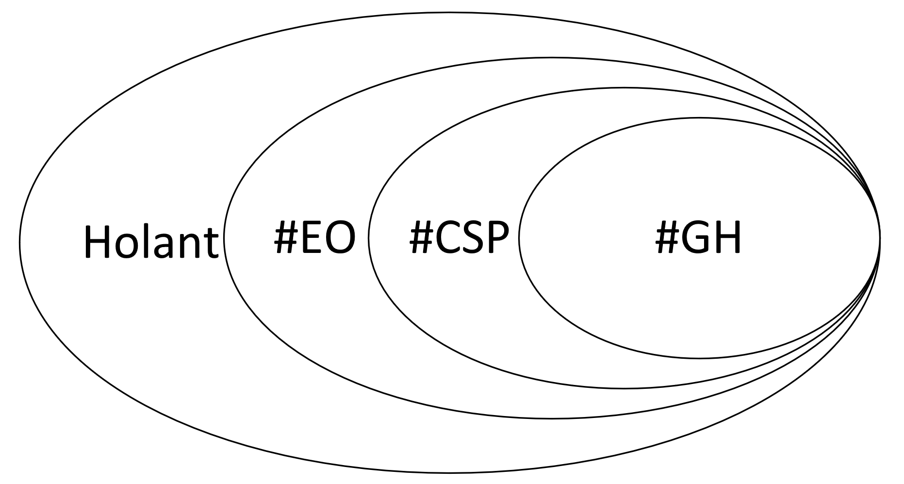
Figure 1: The relationship between the counting problems.

We say a framework $A$ is more general than $B$, denoted as $B\preceq A$ if each problem in $B$ can be transformed into a problem in $A$ in polynomial time. The relationship between these definitions are concluded in the following lemma and Figure 1.

Lemma 1.5.

$$\#\textsf{GH}\preceq\#\textsf{CSP}\preceq\#\textsf{EO}\preceq\textsf{Holant}$$

We delay the proof of Lemma 1.5 to Section 2.2. Besides, Holant is a strictly more general class than $\#\textsf{GH}$, given the fact that counting perfect matchings cannot be represented by a $\#\textsf{GH}$ problem [18] while can be expressed as a Holant problem.

However, the dichotomy for complex weighted Holant problems remains unsettled. There are several constructive attempts on this problem over Boolean domain. A complete dichotomy is established when all signatures are symmetric [19], where a signature is called symmetric when all of its values on the inputs with the same number of 1’s are the same. When signatures aren’t all symmetric, complete dichotomies have been proven for nonnegative signatures [34] and real signatures [37]. Also there are dichotomies for several special forms of Holant problems such as $\textsf{Holant}^{*}$ [22], $\textsf{Holant}^{+}$ [2] and $\textsf{Holant}^{c}$ [1] with some given auxiliary signatures, even complex weighted.

1.2 Motivations

There are two motivations for studying $\#\textsf{EO}$ problems. Firstly, specific forms of $\#\textsf{EO}$ problems appears in many areas like statistic physics and combinatorics. In statistic physics, the ice-type model and the six-vertex model [36] are both special cases of $\#\textsf{EO}$ problems. The latter model, in particular, has emerged as a prominent focus within the broader domain of statistical physics, and is exactly $\#\textsf{EO}$ defined on 4-regular graphs. In the field of combinatorics, the resolution of the Alternating Sign Matrix conjecture [3] and the evaluation of the Tutte polynomial at (3,3) [33] are both related to $\#\textsf{EO}$ problems defined on specific graphs by specific signatures.

Secondly, we conjecture that it’s one of the inevitable problems to be settled towards the complete dichotomy for complex Holant problems. The significance of EO-signature was originally noticed in [19] when discovering the class of vanishing signatures. Also in [34], it’s noticeable that the classification of $\#\textsf{EO}$ problems can compensate the tensor decomposition lemma for complex weighted signatures. Most directly in [37], the research of corresponding $\#\textsf{EO}$ problems (defined by signatures with ARS property), which is previously done in [15], is a vital part of the proof of the dichotomy for real Holant problems. Tending to establish complete complexity classifications for complex Holant problems, we think some of its essential obstacles is hidden in complex $\#\textsf{EO}$ problems.

1.3 Our results

Our first result is stated as follows.

Theorem 1.6.

The $\#\textsf{EO}$ problem defined by $\mathcal{F}$, where $\mathcal{F}$ is a finite set of EO signatures with arity less or equal than 4, is either polynomial time computable or #P-hard. The classification criterion is explicit.

The formal and detailed version of this theorem is Theorem 3.1, and we remark that the form of the tractable cases are not trivial compared to that in the dichotomy for six-vertex model. The idea of analyzing signatures with smaller arity is widely used in the research of counting problems. In order to find the complete complexity classification for $\#\textsf{EO}$ problems, we consider Theorem 1.6 as a solid basis. This is because an EO signature $f$ with arity more than 4 is able to generate different kinds of quaternary and binary signatures through gadget construction.

Our second result focuses on pure signatures. Consider the affine span of the support of a signature $f$. If it’s contained in $\text{HW}^{\geq}$ (or resp. $\text{HW}^{\leq}$), we call $f$ a pure-up (or resp. pure-down) signature.

Suppose $f$ is an EO signature of arity $2d$ and $P=\{\{x_{i_{1}},x_{i_{2}}\},\{x_{i_{3}},x_{i_{4}}\},\cdots,\{x_{i_{2d-1}},x_{i_{2d}}\}\}$ is a pairing of its variables. We define $\textsf{EO}^{P}$ as a subset of $\{0,1\}^{2d}$ decided by $P$, by

$$\textsf{EO}^{P}=\{\alpha\mid\alpha\in\{0,1\}^{2d},\alpha_{i_{1}}\neq\alpha_{i_{2}},\cdots,\alpha_{i_{2d-1}}\neq\alpha_{i_{2d}}\}.$$

If $\text{supp}(f)\subseteq\textsf{EO}^{P}$, we say $f$ is an $\textsf{EO}^{P}$ signature, corresponding to this fixed $P$. The restriction of $f$ to $\textsf{EO}^{P}$ is denoted by $f|_{\textsf{EO}^{P}}$.

There are two important tractable sets $\mathscr{A}$ and $\mathscr{P}$ in the dichotomy for $\#\textsf{CSP}$ problems [23]. If for any $P$, $f|_{\textsf{EO}^{P}}\in\mathscr{A}$ (or resp. $\mathscr{P}$), we say $f$ is $\textsf{EO}^{\mathscr{A}}$ (or resp. $\textsf{EO}^{\mathscr{P}}$). Our second theorem is stated as follows.

Theorem 1.7.

The $\#\textsf{EO}$ problem defined by $\mathcal{F}$, where $\mathcal{F}$ is a finite set of pure-up (pure-down) EO signatures, is polynomial time computable if each $f$ in $\mathcal{F}$ is $\textsf{EO}^{\mathscr{A}}$, or each of them is $\textsf{EO}^{\mathscr{P}}$, otherwise #P-hard.

At last we define a property named rebalancing. Intuitively speaking, 0 (or 1)-rebalancing is that when fixing some variables of a signature $f$ to 0 (or 1), there will be equal number of variables naturally fixed to 1 (or 0), that is it can spontaneously balance the number of 0’s and 1’s in its input strings that give non-zero evaluations. A polynomial time algorithm for this kind of signatures along with some other conditions is presented, which is the most important algorithm in this paper.

Theorem 1.8.

The $\#\textsf{EO}$ problem defined by a finite set $\mathcal{F}$ is polynomial time computable, if every $f\in\mathcal{F}$ is 0-rebalancing (or 1-rebalancing), and all of them are $\textsf{EO}^{\mathscr{A}}$ or $\textsf{EO}^{\mathscr{P}}$ at the same time.

1.4 Our methods

As presented in Section 1.3, there are three parts in this article. In each part, the main subject for us is to characterize different kinds of signature sets. In fact, the main obstacle for us is to give a description for the tractable cases that is precise enough to capture all the tractability. After this characterization, we prove the tractability and the #P-hardness part respectively to achieve a dichotomy.

In each part, we undertake a detailed characterisation of the signature sets, including a comprehensive classification and a rigorous examination of their properties. In particular, we focus on the closure property, the property of the affine span, and the reducibility of the signature.

We also summarize that, for each tractable case in this article, it satisfies two kinds of requirements, namely the nice structure requirement and the type requirement. The nice structure requirement asks that the supports of each signature should have a specific form. This form enables a sending and receiving mechanism, which is necessary for the corresponding algorithm. The type requirement asks that after applying the sending and receiving mechanism to the instance, the set of all the obtained signatures should form a tractable case in $\#\textsf{CSP}$. See Section 3 for a detailed analysis.

We also prove #P-hardness based on the dichotomy of the six-vertex model and that of $\#\textsf{CSP}$, mainly by gadget construction introduced in Section 2.3.

1.5 Organization

In Section 2, we introduce preliminaries needed in our proof. We present the detailed version of our main theorem in Section 3, along with some motivations and observations about the dichotomies. In Section 4, 5 and 6, we give the proofs of Theorem 1.6, 1.7 and 1.8 respectively.

2 Preliminaries

2.1 Definitions and notations

A Boolean variable takes values from a Boolean domain composed of two symbols $\{0,1\}$. Interestingly, sometimes we need to look it as $\mathbb{F}_{2}$, the finite filed of size 2, to characterize special tractable classes of signatures. A signature $f$ with $r$ variables is a mapping from $\{0,1\}^{r}$ to $\mathbb{C}$. The value of $f$ on an input $\alpha$ is denoted as $f_{\alpha}$ or $f(\alpha)$. The set of all $f$’s variables is denoted by $\text{Var}(f)$, and its size is denoted by $\text{arity}(f)$. The support of $f$, denoted by $\text{supp}(f)$, is the set of all inputs on which $f$ is non-zero.

For a $01$-string $\alpha$, we use $\bar{\alpha}$ to denote the dual string of $\alpha$, which is obtained by flipping every bit of $\alpha$. And for $s\in\{0,1\}$, we use $\#_{s}(\alpha)$ to denote the number of $s$’s in $\alpha$. Under this notation we have

$$\text{HW}^{=}=\{\alpha\mid\#_{1}(\alpha)=\#_{0}(\alpha)\},\text{HW}^{\geq}=\{\alpha\mid\#_{1}(\alpha)\geq\#_{0}(\alpha)\}.$$

A signature $f$ is a $\text{HW}^{=}$ signature, which is exactly an EO signature, if $\text{supp}(f)\subseteq\text{HW}^{=}$. The name “EO signature” is originally used in [15] to briefly denote Eulerian Orientation signature. If $\text{supp}(f)\subseteq\text{HW}^{\geq}$, we call $f$ an $\text{HW}^{\geq}$ signature. There are other similar notations, which replace “$\geq$”, by “$\leq$”, “$<$”, or “$>$” in names and defining formulae.

For a set $S$ of 01-strings of length $k$, the affine span of $S$ is the minimum affine subspace containing $S$. For a signature $f$, we use $\text{Span}(f)$ to denote the affine span of $\text{supp}(f)$.

We use $[f_{0},f_{1},\ldots,f_{r}]$ to denote a symmetric signature $f$ with arity $r$, giving evaluation $f_{i}$ on all input strings of Hamming weight $i$. Exchanging the names of the symbols in the Boolean domain, we can get $f$’s dual signature $\widetilde{f}=[\widetilde{f}_{0},\widetilde{f}_{1},\ldots,\widetilde{f}_{r}]=[f_{r},f_{r-1},\ldots,f_{0}]$. If $f=\widetilde{f}$, $f$ is said to be a self-dual signature. $\Delta_{0}$ denotes the unary signature $[1,0]$, while its dual is $\Delta_{1}=[0,1]$. We use $\neq_{2}$ to denote the binary disequality signature $[0,1,0]$, and it is an example of self-dual signature. The meaning of “dual” and “self-dual” can be naturally generalized to asymmetric signatures, sets of signatures, Boolean domain counting problems and tractable classes in dichotomy theorems. We use $\otimes$ to denote the tensor multiplication.

We use $[\varphi]$ to denote the logic value of a sentence $\varphi$. It has a value from $\{\text{True},\text{False}\}$, or the isomorphic integer set $\{1,0\}$. For example, $[x\neq y]$ is True (or 1) when $x\neq y$, otherwise it’s False (or 0). Hence, both $[x\neq y]$ and $\neq_{2}(x,y)$ express the value of the binary function $\neq_{2}$ on $(x,y)$.

There are several sets of frequently used signatures. We use $\mathcal{EQ}$ to denote the set of equality signatures that $\mathcal{EQ}=\{=_{1},=_{2},\cdots\,=_{r},\cdots\}$, where $=_{r}$ denotes an arity $r$ signature $[1,0,\ldots,0,1]$. In other words, $=_{r}$ takes value 1 when the input is pure 0 or 1, otherwise takes value 0 instead.

A disequality signature of arity $2d$, denoted by $\neq_{2d}$, takes value 1 when $x_{1}=x_{2}=\cdots=x_{d}\neq x_{d+1}=x_{d+2}=\cdots=x_{2d}$, otherwise takes value 0 instead. We let $\mathcal{DEQ}=\{\neq_{2},\neq_{4},\cdots,\neq_{2n},\cdots\}$ be the set of all disequality signatures. Furthermore, $\mathcal{DEQ}$ is also defined to be closed under variable permutation. In other words, suppose $\pi\in S_{2d}$ and a signature $f$ takes value 1 when $x_{\pi(1)}=x_{\pi(2)}=\cdots=x_{\pi(d)}\neq x_{\pi(d+1)}=x_{\pi(d+2)}=\cdots=x_{\pi(2d)}$, otherwise takes value 0 instead. Then $f$ is also considered as a disequality signature.

There is an alternative definition of disequality signatures. If $f$ is an EO signature of arity $2d$ and there exists an $\alpha\in\text{HW}^{=}$ such that $\text{supp}(f)=\{\alpha,\bar{\alpha}\}$ and $f(\alpha)=f(\bar{\alpha})=1$, then $f$ is a disequality signature. It can be easily verified that two definitions are equivalent.

Similarly, if $f$ is an EO signature of arity $2d$ and there exists an $\alpha\in\text{HW}^{=}$ such that $\text{supp}(f)=\{\alpha,\bar{\alpha}\}$ and $f(\alpha)=a,f(\bar{\alpha})=b$, then $f$ is a generalized disequality signature, denoted by $\neq_{2d}^{a,b}$,

2.2 Relationships between counting problems

In this section, we aim to give a detailed characterization of counting problems in Section 1.1 by proving Lemma 1.5. We use $\leq_{T}$ and $\equiv_{T}$ to respectively denote polynomial-time Turing reductions and equivalences.

By Definition 1.1 to 1.4, it is easy to verify the following lemma.

Lemma 2.1.

$\#\textsf{GH}(f)\equiv_{T}\#\textsf{CSP}(\{f\}).$

Lemma 2.2.

[15] $\#\textsf{EO}(\mathcal{F})\equiv_{T}\textsf{Holant}(\neq_{2}\mid\mathcal{F})$.

We also have the following lemma from [37].

Lemma 2.3.

[37] $\textsf{Holant}(\neq_{2}\mid\mathcal{F})\equiv_{T}\textsf{Holant}(Z^{-1}\mathcal{F})$

Here, $Z^{-1}=\frac{1}{\sqrt{2}}\left(\begin{matrix}1&-\mathfrak{i}\\ 1&\mathfrak{i}\end{matrix}\right)$, and $Z^{-1}\mathcal{F}$ is the signature set obtained from $\mathcal{F}$ by taking a holographic transformation [38, 14] defined by $Z^{-1}$. We omit the introduction of holographic transformation and the proof of this lemma, as they do not play a key role in this article. However, readers are encouraged to have a better understanding of holographic transformation from [9][Section 1.3.2] as holographic transformation is a very powerful method in the field of counting complexity.

Suppose $f$ is an EO signature of arity $2d$, with variable set $\text{Var}(f)=\{x_{1},x_{2},\cdots,x_{2d}\}$. Fix an arbitrary perfect pairing $P=\{\{x_{i_{1}},x_{i_{2}}\},\{x_{i_{3}},x_{i_{4}}\},\cdots,\{x_{i_{2d-1}},x_{i_{2d}}\}\}$ of $\text{Var}(f)$. We define $\textsf{EO}^{P}$ as a subset of $\{0,1\}^{2d}$ corresponding to $P$, by

$$\textsf{EO}^{P}=\{\alpha\mid\alpha\in\{0,1\}^{2d},\alpha_{i_{1}}\neq\alpha_{i_{2}},\cdots,\alpha_{i_{2d-1}}\neq\alpha_{i_{2d}}\},$$

or equivalently, $\textsf{EO}^{P}=\text{supp}([x_{i_{1}}\neq x_{i_{2}}]\cdot[x_{i_{3}}\neq x_{i_{4}}]\cdots[x_{i_{2d-1}}\neq x_{i_{2d}}]).$

If $\text{supp}(f)\subseteq\textsf{EO}^{P}$, we say $f$ is an $\textsf{EO}^{P}$ signature, corresponding to this fixed $P$. If there exists some perfect pairing $P$ of $\text{Var}(f)$ such that $f$ is an $\textsf{EO}^{P}$ signature, we say $f$ is a pairwise opposite signature (exactly as Definition 5.5 in [15]), or an $\textsf{EO}^{\text{M}}$ signature for short.

For an $\textsf{EO}^{P}$ signature $f$ defined above, we define $\tau_{f}$, also denoted as $\tau(f)$, as a set of arity $d$ signatures such that

$$\tau_{f}(P)=\{g\mid g(x_{j_{1}},x_{j_{3}},...,x_{j_{2d-1}})=f(x_{i_{1}},1-x_{i_{1}},x_{i_{3}},1-x_{i_{3}},\ldots,x_{i_{2d-1}},1-x_{i_{2d-1}}),$$

$$x_{j_{1}}\in\{x_{i_{1}},x_{i_{2}}\},\cdots,x_{j_{2d-1}}\in\{x_{i_{2d-1}},x_{i_{2d}}\}\}.$$

Since $P$ can exchange the positions of two variables in one pair freely, we know that $|\tau_{f}|=2^{d}$.

We then define the “inverse mapping” of $\tau$. Let $g$ be an arbitrary signature of arity $d$. We define $\pi(g)$, also denoted as $\pi_{g}$, as

$$\pi_{g}(x_{1},y_{1},x_{2},y_{2},\ldots,x_{d},y_{d})=g(x_{1},x_{2},\ldots,x_{d})\cdot[x_{1}\neq y_{1}]\cdots[x_{d}\neq y_{d}].$$

Obviously, $\pi_{g}$ is an $\textsf{EO}^{P}$ signature with $P=\{\{x_{1},y_{1}\},\{x_{2},y_{2}\},\cdots,\{x_{d},y_{d}\}\}$. We also define $\pi(\mathcal{F})=\{\pi(f)\mid f\in\mathcal{F}\}$. $\tau(\pi(g))$ contains $g$. In fact, it is composed of all signatures that can be realized by flipping some variables of $g$ using the binary disequality. This hints that $\#\textsf{EO}$ is equivalent to $\#\textsf{CSP}$ with free binary disequality.

With a more detailed argument in [15], including the equivalence of computational complexity between $\#\textsf{CSP}$ and $\#\textsf{CSP}$ with free binary disequality, the following stronger lemma can be obtained.

Lemma 2.4.

[15, Theorem 6.1] $\#\textsf{CSP}(\mathcal{F})\equiv_{T}\#\textsf{EO}(\pi(\mathcal{F})).$

Combining Lemma 2.1-2.4, Lemma 1.5 is proved.

2.3 Gadget construction and signature matrix

This subsection presents two important concepts, namely gadget construction and signature matrix. Gadget construction is a fundamental method for reduction in complexity classification. The signature matrix provides us a more intuitive overview of a signature, and establish the association between gadget construction and matrix multiplication.

Given $\mathcal{F}$ as a set of signatures, an $\mathcal{F}$-gate is similar to a signature grid $\Omega(G,\pi)$ in Definition 1.3, except that $G=(V,E,D)$ instead. Here, $V$ is the set of vertices, $E$ is the set of internal edges and $D$ is the set of dangling edges. Each edge in $E$ is adjacent to two vertices in $V$, while each edge in $D$ is adjacent to a single vertex in $V$. An $\mathcal{F}$-gate is essentially a signature, whose variables are represented by edges in $D$. Suppose $|E|=n$ and $|D|=m$, and edges in $E$ represent variables $\{x_{1},x_{2},\cdots,x_{n}\}$ while edges in $D$ represent variables $\{y_{1},y_{2},\cdots,y_{m}\}$. Then the $\mathcal{F}$-gate defines a signature $f$ that

$$f(y_{1},y_{2},\cdots,y_{m})=\sum_{\sigma:E\rightarrow\{0,1\}}\prod_{v\in V}f_{v}(\hat{\sigma}|_{E(v)}),$$

where $(y_{1},y_{2},\cdots,y_{n})\in\{0,1\}^{n}$ is an assignment on variables represented by dangling edges, $\hat{\sigma}$ is the extension of $\sigma$ by the assignment of $(y_{1},y_{2},\cdots,y_{n})$. $f$ is called the signature of this $\mathcal{F}$-gate. We say that a signature $f$ is realizable from a set $\mathcal{F}$ by gadget construction when $f$ is the signature of an $\mathcal{F}$-gate. In particular, there may be no internal edges in an $\mathcal{F}$-gate. At this situation, the signature represented by this $\mathcal{F}$-gate is basically the tensor product of several signatures. It is worth noticing that if $f$ is realizable by $\mathcal{F}$, naturally by [9, lemma 1.3] we have

$$\textsf{Holant}(\mathcal{F})\equiv_{T}\textsf{Holant}(\mathcal{F}\cup\{f\})$$

In the setting of $\#\textsf{EO}$ problems we have a slightly different way to define $\mathcal{F}$-gate. Since $\#\textsf{EO}(\mathcal{F})\equiv_{T}\textsf{Holant}(\neq_{2}\mid\mathcal{F})$ by Lemma 2.2, we only need to add an extra vertex assigned $\neq_{2}$ to each internal edge, and similarly calculate all values of $f$ by seeing it as a normal gate in the setting of Holant problems. In the rest part of this paper, when we analyze problems in the setting of $\#\textsf{EO}$ problems, $\mathcal{F}$-gate is defined this way by default without causing ambiguity.

Next, we introduce the matrix form of signatures. Essentially, it’s an orderly and reasonable way to list all possible values of a signature. Suppose $f$ is an arbitrary signature that is a mapping from $\{0,1\}^{r}$ to $\mathbb{C}$. First we give an order for all variables of $f$, say $x_{1},x_{2},\cdots,x_{r}$. The matrix form of $f$ (or signature matrix of $f$ [9]) with parameter $l$ is a $2^{l}\times 2^{r-l}$ matrix for some integer $0\leq l\leq r$, where values of $x_{1},x_{2},\cdots,x_{l}$ forms the row index and values of $x_{l+1},x_{l+2},\cdots,x_{r}$ forms the column index. The matrix is denoted as $M(f)_{x_{1}x_{2}\cdots x_{l},x_{l+1}x_{l+2}\cdots x_{r}}$. Sometimes for convenience we omit the symbol $(f)$ and sometimes we denote the signature matrix as $M_{f}$ without causing ambiguity. For an even arity signature we usually let $l=\frac{r}{2}$.

Example 2.5 (Signature matrix).

If $f$ is a binary signature and $f=(f_{00},f_{01},f_{10},f_{11})$, then $M_{f}=M_{x_{1},x_{2}}=\left(\begin{matrix}f_{00}&f_{01}\\ f_{10}&f_{11}\end{matrix}\right)$.

If $g$ is a quaternary signature, then

$$M_{g}=M_{x_{1}x_{2},x_{3}x_{4}}=\left(\begin{matrix}g_{0000}&g_{0001}&g_{0010}&g_{0011}\\ g_{0100}&g_{0101}&g_{0110}&g_{0111}\\ g_{1000}&g_{1001}&g_{1010}&g_{1011}\\ g_{1100}&g_{1101}&g_{1110}&g_{1111}\end{matrix}\right).$$

We now introduce the relation between matrix multiplication and gadget construction. Suppose $f$ and $g$ are $\mathcal{F}$-gates, given some $\mathcal{F}$. $f$ has arity $n$ while $g$ has arity $m$. Suppose $\text{Var}(f)=\{x_{1},x_{2},\cdots,x_{n}\}$ and $\text{Var}(g)=\{y_{1},y_{2},\cdots,y_{m}\}$. We now construct a new gadget by connecting part of $f$ and $g$’s dangling edges, say $\{x_{n-l+1},\cdots,x_{n}\}$ respectively with $\{y_{1},y_{2},\cdots,y_{l}\}$, where $l\in\mathbb{Z}_{+}$. The new signature $h$ is still an $\mathcal{F}$-gate by definition. $\text{Var}(h)=\{x_{1},\cdots,x_{n-l},y_{l+1},\cdots,y_{m}\}$ and by comparing the computation of gadget construction to matrix multiplication we have

$$M_{h}=M_{x_{1}\cdots x_{n-l},y_{l+1}\cdots y_{m}}=M_{x_{1}\cdots x_{n-l},x_{n-l+1}\cdots x_{n}}\cdot M_{y_{1}\cdots y_{l},y_{l+1}\cdots y_{m}}=M_{f}\cdot M_{g}.$$

It should be clarified that in the setting of $\#\textsf{EO}$ problems, the only difference is that all edges represent $\neq_{2}$ instead of $=_{2}$. As a result, we have

$$M_{h}=M_{f}\cdot\neq_{2}^{\otimes l}\cdot M_{g},$$

which will be frequently used without detailed explanations in the following.

There are two special forms of gadget construction we need to emphasize, namely self-loop and pinning. In the setting of $\#\textsf{EO}$, adding a self-loop on a signature $f$ means choosing two variables of $f$, namely $x_{1}$ and $x_{2}$, and adding an internal edge between them to get a new signature $f^{x_{1}\neq x_{2}}$. Suppose $\text{Var}(f)=\{x_{1},x_{2},\cdots,x_{n}\}$. As the internal edge represents a $\neq_{2}$ signature, we have

$$f^{x_{1}\neq x_{2}}(x_{3},\cdots,x_{n})=f(0,1,x_{3},\cdots,x_{n})+f(1,0,x_{3},\cdots,x_{n}).$$

It can be verified through the definition of $\mathcal{F}$-gate that gadget construction can be seen equivalently as a combination of tensor multiplication and adding self-loops. Besides, if $f$ is of arity 2, the result of adding a self-loop will be a complex number, which is also the partition function of this simple signature grid.

We can generalize this operation by using $\neq_{2}^{a,b}$. Adding a self-loop on $f$ by $\neq_{2}^{a,b}$ is a similar operation as before, except that we don’t add an internal edge between $x_{1}$ and $x_{2}$, but add an extra vertex assigned $\neq_{2}^{a,b}$ and two internal edges respectively connecting $x_{1}$, $x_{2}$ with $\neq_{2}^{a,b}$’s dangling edges. It can be seen as a weighted self-loop. Noticing that there are two ways to add internal edges, we can get either $f^{\prime}(x_{3},\cdots,x_{n})=af(0,1,x_{3},\cdots,x_{n})+bf(1,0,x_{3},\cdots,x_{n})$ or $f^{\prime}(x_{3},\cdots,x_{n})=bf(0,1,x_{3},\cdots,x_{n})+af(1,0,x_{3},\cdots,x_{n})$.

The second form we need to emphasize is pinning. It’s well-known in the setting of Holant or $\#\textsf{CSP}$ problems that pinning means fixing one variable to 0 or 1, using $\Delta_{0}=(1,0)$ or $\Delta_{1}=(0,1)$. Here in the setting of $\#\textsf{EO}$ problems pinning is adding a self-loop by $\neq_{2}^{1,0}$. Suppose $x,y\in\text{Var}(f)$ and by the pinning operation we can fix $x$ to 1 and $y$ to 0. The resulting signature is denoted as $f^{x=1,y=0}$. Pinning here essentially fix two variables to opposite values at the same time, and keeps the EO property of a signature. In this paper, without causing ambiguity, when we refer to the pinning signature, we mean $\neq_{2}^{1,0}$.

2.4 Two known dichotomies for #CSP and Six-vertex model

In this section, we introduce the dichotomies for $\#\textsf{CSP}$ and six-vertex model. We start from defining tractable classes $\mathscr{A}$ and $\mathscr{P}$. Let $X$ be a $(d+1)$-dimensional column vector $X=(x_{1},x_{2},\cdots,x_{d},1)^{T}$ over $\mathbb{F}_{2}$. Suppose $A$ is a matrix over $\mathbb{F}_{2}$. The function $\chi_{AX}$ takes value 1 when $AX=\mathbf{0}$, otherwise 0. In other words, $\chi_{AX}$ describe an affine relation on variables $x_{1},x_{2},\cdots,x_{d}$.

Definition 2.6.

[23] We denote by $\mathscr{A}$ the set of signatures which have the form $\lambda\cdot\chi_{AX}\cdot\mathfrak{i}^{L_{1}(X)+L_{2}(X)+\cdots+L_{n}(X)}$, where $\mathfrak{i}=\sqrt{-1}$, $\lambda\in\mathbb{C}$, $n\in\mathbb{Z}_{+}$, each $L_{j}$ is a 0-1 indicator function of the form $\langle\alpha_{j},X\rangle$, where $\alpha_{j}$ is a $(d+1)$-dimensional vector over $\mathbb{F}_{2}$, and the dot product $\langle\cdot,\cdot\rangle$ is computed over $\mathbb{F}_{2}$.

Definition 2.7.

[23] We denote by $\mathscr{P}$ the set of all signatures which can be expressed a product of unary signatures, binary equality signatures ($=_{2}$) and binary disequality signatures ($\neq_{2}$) (on not necessarily disjoint subsets of variables).

As in [9, chapter 3], $\mathscr{A}$ and $\mathscr{P}$ are close under gadget construction. That is, if $\mathcal{F}\subseteq\mathscr{A}$ or $\mathcal{F}\subseteq\mathscr{P}$, then all $\mathcal{F}$-gates are respectively in $\mathscr{A}$ or $\mathscr{P}$. Now we state the dichotomy for $\#\textsf{CSP}$ from [23, theorem 3.1].

Theorem 2.8.

[23] Suppose $\mathcal{F}$ is a finite set of signatures mapping Boolean inputs to complex numbers. If $\mathcal{F}\subseteq\mathscr{A}$ or $\mathcal{F}\subseteq\mathscr{P}$, then $\#\textsf{CSP}(\mathcal{F})$ is computable in polynomial time. Otherwise, $\#\textsf{CSP}(\mathcal{F})$ is #P-hard.

Now we introduce some definitions for the dichotomy for six-vertex model. $\mathscr{M}$ is the set of all ternary signatures whose supports only contain strings of Hamming weight exactly 1. In other words, a quaternary EO signature $f\in\mathscr{M}\otimes\Delta_{1}$, if and only if $\text{supp}(f)\subseteq\{1\}\times\{100,010,001\}=\{1100,1010,1001\}$. $\widetilde{\mathscr{M}}$ is defined similarly, except that the Hamming weights of the supports are exactly 2. The dichotomy for six-vertex model is as follows.

Theorem 2.9.

[17] Let f be a quaternary EO signature, then $\textsf{Holant}(\neq_{2}\mid f)$ is #P-hard except for the following cases:

a. $f\in\mathscr{P}$ (equivalently, $f\in\textsf{EO}^{\text{M}}$ and $\tau(f)\subseteq\mathscr{P}$);

b. $f\in\mathscr{A}$ (equivalently, $f\in\textsf{EO}^{\text{M}}$ and $\tau(f)\subseteq\mathscr{A}$);

c. $f\in\mathscr{M}\otimes\Delta_{1}$;

d. $f\in\widetilde{\mathscr{M}}\otimes\Delta_{0}$;

in which cases $\textsf{Holant}(\neq_{2}\mid f)$ is computable in polynomial time.

We summarize current notations as the following tree. The child node can be seen as a subset of the parent node.

2.5 Observations

Starting from this section, this article presents a number of observations pertaining to the tractable cases within each dichotomy. The objective is to generalize these tractable cases at a high level of abstraction, although some statements may be informal. It is our hope that these generalized characteristics, derived from the tractable cases, will prove a valuable point of reference for future research.

In the dichotomy of $\#\textsf{CSP}$, both $\mathscr{A}$ and $\mathscr{P}$ are self-dual signature sets. All signatures in $\mathscr{A}$ and $\mathscr{P}$ have affine supports, so having affine support is a necessary condition for tractability here, and we consider this condition as a nice structure requirement. Informally speaking, there are two ways to reach tractability based on the nice structure requirement. Informally speaking, $\mathscr{A}$ type and $\mathscr{P}$ type are two sets meeting different additional requirements to reach tractability in the setting of $\#\textsf{CSP}$ problems. $\mathscr{A}$ type requires further restrictions on weights of signatures, while $\mathscr{P}$ type requires a more restricted and special kind of affine supports. The two steps explanation for the tractability part in Theorem 2.8, will be used as an important template in explaining the following dichotomies. We hope to exhibit an informal evolution process from the known tractable cases to the new tractable cases in this way.

In the dichotomy for six-vertex model, the nice structure requirement is from two different parts. The first part is an inheritance of affine support condition from Theorem 2.8, as observed in [17], that a special kind of EO signatures’ supports in the $\#\textsf{EO}$ setting can simulate $\#\textsf{CSP}$, as described in Lemma 2.4.

A direct corollary of Theorem 2.8 and Lemma 2.4, is already a mini dichotomy for $\#\textsf{EO}$ problems defined by $\textsf{EO}^{\text{M}}$ signatures, where there are two tractable classes. Suppose $\mathcal{F}$ is a set of $\textsf{EO}^{\text{M}}$ signatures. Then $\#\textsf{EO}(\mathcal{F})$ is tractable if for each $f\in\mathcal{F}$, $\tau(f)\subseteq\mathscr{A}$, or for each $f\in\mathcal{F}$, $\tau(f)\subseteq\mathscr{P}$; otherwise it is #P-hard. The nice structure requirement shared by both tractable classes is that each $f\in\mathcal{F}$ is $\textsf{EO}^{\text{M}}$ and supports of all signatures in $\tau(f)$ are affine. This requirement is equivalent to that $f$ is EO and $\text{supp}(f)$ is affine by the following lemma.

Lemma 2.10.

[15, Lemma 5.7] If an EO signature $f$ has affine support, then $f$ is a pairwise opposite signature ($\textsf{EO}^{\text{M}}$ signature).

Lemma 2.11.

[15] $f\in\mathscr{A}$ (resp. $\mathscr{P}$) if and only if $\tau(f)\subseteq\mathscr{A}$ (resp. $\mathscr{P}$).

Coming back to quaterany EO signatures, the above analysis implies the following. The first part of the nice structure requirement of six-vertex model, is that the support must be an affine subspace, and regardless of variable permutations, an affine subspace of $Q=\{0101,1001,0110,1010\}$. This corresponds to the tractable cases a and b in Theorem 2.9.

The second part of the nice structure requirement of six-vertex model, is that the support must be an subset of $Q_{1}=\{1100,1010,1001\}$ or its dual, $Q_{0}=\{0011,0101,0011\}$. This requirement itself is enough for tractability.

The set $Q_{1}=\{1100,1010,1001\}\subseteq\{0,1\}^{\{x_{1},x_{2},x_{3},x_{4}\}}$ is a nice structure related to the stable $\textsf{EO}^{\text{M}}$ type support requirement. Noticing that if each signature $f$ in the instance satisfies that $\text{supp}(f)=Q_{1}$, then one of its variables is fixed to 1, say $x_{1}$. Transmitted by $\neq_{2}$, as well as the general binary disequality signatures in the instance, another edge $x_{2}$ of a signature $g$ will be fixed to 0. Then the valid part of $\text{supp}(g)$, that is the set of strings that can appear in the assignment which gives non-zero evaluation, is now a set of at most two strings and meets $\textsf{EO}^{\text{M}}$ type affine support requirement. We denote this process as the sending and receiving mechanism. This process may repeat many rounds, until each signature collapses to $\textsf{EO}^{\text{M}}$. At each round, an opposite pair of variables is somehow fixed by this mechanism. And the process continues until the rest signatures in the whole instance are in $\textsf{EO}^{\text{M}}$. Hence, this more general nice structure property, can force a signature in an instance to work exactly like some $\textsf{EO}^{\text{M}}$ signature.

The analysis of the dual case $Q_{0}$ is similar.

3 New notations and our results

In this section, we introduce some more notations, and present our results and approaches in details. In Subsection 3.1, we introduce two strange signatures, which serve as a motivation for some of our study. There are three parts of results in this paper, which are introduced in Subsection 3.2, 3.3, 3.4 respectively. Finally in Subsection 3.5 we introduce the relations between these results.

3.1 Two strange signatures

In this subsection we present the definition of $f_{40}$ and $f_{56}$, which are considered as two important cases in our study. Some of our results are motivated by these signatures. We first introduce some notations to describe signatures with large arity and a sparse support.

For matrices $A_{s,p}$ and $B_{s,q}$, we use $C_{s,p+q}=(A\oplus B)$ to denote the matrix $C$ satisfying

$$C(i,j)=\begin{cases}A(i,j),&1\leq j\leq p;\\ B(i,j-p),&p+1\leq j\leq p+q.\end{cases}$$ (1)

Informally speaking, $C$ is a connection of $A,B$. We use $A^{\oplus k}$ to denote the matrix $A\oplus...\oplus A$, which is a connection of $k$ copies of matrix $A$. We also define the following matrices.

$$H_{0}=\begin{pmatrix}0\\ 0\\ 0\\ 0\\ 0\\ \end{pmatrix},H_{2}=\begin{pmatrix}1&1&1&1&0&0&0&0&0&0\\ 1&0&0&0&1&1&1&0&0&0\\ 0&1&0&0&1&0&0&1&1&0\\ 0&0&1&0&0&1&0&1&0&1\\ 0&0&0&1&0&0&1&0&1&1\\ \end{pmatrix},H_{4}=\begin{pmatrix}0&1&1&1&1\\ 1&0&1&1&1\\ 1&1&0&1&1\\ 1&1&1&0&1\\ 1&1&1&1&0\\ \end{pmatrix}$$

For a signature $f$ of arity $k$, we use the support matrix $R_{s,k}$ to describe its support. A string $\alpha\in\{0,1\}^{k}$ is a support of $f$ if and only if $\alpha$ equals a row in $R_{s,k}$. $f_{40}$ has the support matrix $R_{40}=H_{2}^{\oplus 3}\oplus H_{4}^{\oplus 2}$, $f_{56}$ has the support matrix $R_{56}=H_{0}\oplus H_{2}^{\oplus 4}\oplus H_{4}^{\oplus 3}$ and both of them take value in $\{0,1\}$. Though the supports of them are sparse, they are not able to be captured by a number of existing algorithms and hardness results.

3.2 A set of binary or quaternary signatures

The first part of our results generalizes six-vertex model to $\#\textsf{EO}$ problems defined by a set of EO signatures of arity no more than 4. We define

$$\mathscr{M}_{\mathscr{A}}=\{f\in\mathscr{M}\mid\text{the quotient of any two non-zero values of }f\text{ belongs to }\{\pm 1,\pm\mathfrak{i}\}\}.$$

$\mathscr{M}_{\mathscr{A}}\otimes\Delta_{1}$ can be seen as $\mathscr{M}\otimes\Delta_{1}$ with the $\mathscr{A}$ type requirement. Similarly, we define

$$\widetilde{\mathscr{M}_{\mathscr{A}}}=\{f\in\widetilde{\mathscr{M}}|\text{the quotient of }\text{any two }\text{non-zero values }\text{of f }\text{belongs to }\{\pm 1,\pm\mathfrak{i}\}\}.$$

The detailed version of Theorem 1.6 is as follows.

Theorem 3.1.

Suppose $\mathcal{F}$ is a set of Eulerian signatures with arity less than or equal to 4, mapping Boolean inputs to complex numbers. Then $\textsf{Holant}(\neq_{2}\mid\mathcal{F})$ is #P-hard unless one of the following conditions holds:

a. $\mathcal{F}\subseteq\mathscr{P}\cup\mathscr{M}\otimes\Delta_{1}$;

b. $\mathcal{F}\subseteq\mathscr{A}\cup\mathscr{M}_{A}\otimes\Delta_{1}$;

c. $\mathcal{F}\subseteq\mathscr{P}\cup\widetilde{\mathscr{M}}\otimes\Delta_{0}$;

d. $\mathcal{F}\subseteq\mathscr{A}\cup\widetilde{\mathscr{M}_{\mathscr{A}}}\otimes\Delta_{0}$,

in which cases the problem can be computed in polynomial time.

Again, we summarize current notations as the following tree. The child node can be seen as a subset of the parent node, and when a set of signatures can meet all requirements on a path from the root to the four nodes at the bottom, the corresponding $\#\textsf{EO}$ problem is tractable. We also write a specific example of the $\mathscr{A}$ type requirement.

3.2.1 Observation

In this dichotomy, there are two general nice structures dual to each other, which is the restriction on the support of each signature. Each structure, additionally with an $\mathscr{A}$ type requirement or a $\mathscr{P}$ type requirement, can achieve tractability.

In six-vertex model, at the fourth level of the tree above, there are three elements, $Q$, $Q_{1}$ and $Q_{0}$, representing different nice structure requirements of the support. After adding $\mathscr{A}$ type or $\mathscr{P}$ type requirement respectively, $Q$ becomes the first two tractable classes in Theorem 2.9.

However, when the $\mathscr{A}$ type requirement is applied to $Q_{1}$, the obtained signatures satisfy the $\mathscr{P}$ type requirement as well. Consequently, the $\mathscr{P}$ type requirement is a weaker condition, and manifest in the third tractable case of theorem 2.9. However, when we consider a set of signatures, $Q$-support signatures may also exist. Consequently Theorem 3.1 shows the difference between adding the $\mathscr{A}$ type requirement and the $\mathscr{P}$ type requirement.

3.3 Pure signatures

In this section we focus on pure signatures, which can be seen as a generalization of the quaternary signatures in $\mathscr{M}\otimes\Delta_{1}$ and $\widetilde{\mathscr{M}}\otimes\Delta_{0}$.

Definition 3.2.

An EO signature $f$ is pure-up, if $\text{Span}(f)\subseteq\text{HW}^{\geq}$. A signature set $\mathcal{F}$ is a pure-up EO signature, if each signature in it is pure-up. Similarly, An EO signature $f$ is pure-down, if $\text{Span}(f)\subseteq\text{HW}^{\leq}$. A signature set $\mathcal{F}$ is pure-down, if each signature in it is a pure-down EO signature.

Both pure-up and pure-down signatures are collectively referred to as pure signatures.

We summarize current notations as the following tree.

In the following, we present the dichotomy of pure signatures and the corresponding definitions. It is worth noticing that in this section, $\mathcal{F}$ is either pure-up or pure-down.

Definition 3.3.

Suppose $f$ is an arity $2d$ EO signature and $S\subseteq\text{HW}^{=}$. $f|_{S}$ is the restriction of $f$ to $S$, which means when $\alpha\in S$, $f|_{S}(\alpha)=f(\alpha)$, otherwise $f|_{S}(\alpha)=0$.

If for any perfect pairing $P$ of Var$(f)$, $f|_{\textsf{EO}^{P}}\in\mathscr{A}$, then we say that $f$ is $\textsf{EO}^{\mathscr{A}}$.

Similarly, if for any perfect matching $P$ of Var$(f)$, $f|_{\textsf{EO}^{P}}\in\mathscr{P}$, then $f$ is $\textsf{EO}^{\mathscr{P}}$.

Theorem 3.4 (The dichotomy for pure-up EO signatures).

Suppose $\mathcal{F}$ is a set of pure-up EO signatures. Then $\#\textsf{EO}(\mathcal{F})$ is #P-hard unless all signature in $\mathcal{F}$ are $\textsf{EO}^{\mathscr{A}}$ or all of them are $\textsf{EO}^{\mathscr{P}}$.

3.3.1 Observation

In the rest of this section, we focus on pure-up signatures. The analysis of pure-down signatures is similar.

Our motivation comes from a quaternary signature $f$ satisfying $\text{supp}(f)=\{1100,1010,1001\}$. The affine span of $\{1100,1010,1001\}$ is $\{1100,1010,1001,1111\}$, which is contained in $\text{HW}^{\geq}$. We modify $f$ to $f^{\prime}$ by adding a nonzero new value on the input 1111. In [19], it is proved that $\textsf{Holant}(\neq_{2}\mid[0,0,a,b,c])\equiv_{T}\textsf{Holant}(\neq_{2}\mid[0,0,a,0,0])$, by stating all supports in $\text{HW}^{>}$ have no contributions to the partition function. Consequently, $\#\textsf{EO}(f^{\prime})\equiv_{T}\#\textsf{EO}(f)$, and this technique of adding supports is the origin motivation for the study of pure signatures.

When studying the property of pure-up signatures, we prove that a pure-up signature is either $\textsf{EO}^{\text{M}}$, or has at least one variable fixed to 1. This property enables pure signatures to apply the sending and receiving mechanism. In other words, pure signatures imply new nice structure requirement, which has two cases mutually dual to each other while their intersection is the self-dual $\textsf{EO}^{\text{M}}$ structure requirement. Furthermore, each case can reach tractability by additionally adding a new kind of $\mathscr{A}$ type or $\mathscr{P}$ type requirement, which is $\textsf{EO}^{\mathscr{A}}$ or $\textsf{EO}^{\mathscr{P}}$.

We also remark that, the tractable cases in Theorem 3.4 can be seen as a generalization of those in Theorem 3.1.

3.4 Rebalancing signatures

In this section, we define a property named $rebalancing$ for EO signatures.

Definition 3.5 (Rebalancing).

An EO signature $f$ of arity $2d$, is called 0-rebalancing(1-rebalancing respectively), when the following recursive conditions are met.

• $d=0$: No restriction.

• $d\geq 1$: For any variable $x$ in $X=\text{Var}(f)$, there exists a variable $y=\psi(x)$ different from $x$, such that for any $\alpha\in\{0,1\}^{X}$, if $\alpha_{x}=\alpha_{y}=0$($\alpha_{x}=\alpha_{y}=1$ respectively) then $f(\alpha)=0$. Besides, the arity $2d-2$ signature $f^{x=0,y=1}$ is 0-rebalancing($f^{x=1,y=0}$ is 1-rebalancing respectively).

For completeness we view all nontrivial signatures of arity 0, which is a non-zero constant, as 0-rebalancing(1-rebalancing) signatures. For the $d\geq 1$ case, $\psi$ is said to be the first level mapping of $f$.

Tractability can also be obtained based on 0-rebalancing/1-rebalancing property.

Theorem 3.6.

If $\mathcal{F}$ is composed of 0-rebalancing(1-rebalancing) $\textsf{EO}^{\mathscr{A}}$ signatures, or $\mathcal{F}$ is composed of 0-rebalancing(1-rebalancing) $\textsf{EO}^{\mathscr{P}}$ signatures, then $\textsf{Holant}(\neq_{2}\mid\mathcal{F})$ is polynomial time computable.

Now we introduce the relation between 0-rebalancing (1-rebalancing) signatures and two kinds of signatures we have discussed in the above sections.

Remark 3.7.

It’s easy to verified that an $\textsf{EO}^{\text{M}}$ signature is both 0-rebalancing and 1-rebalancing. All pure-up signatures are also 0-rebalancing. Given a pure-up signature, if $\text{supp}(f)\cap\text{HW}^{>}\neq\emptyset$, then it has $\Delta_{1}(x)$ by Lemma 5.1, which naturally gives a first level mapping $\psi$ that the images of all variables except $x$ are $x$, and $\psi(x)$ can be any one except itself. It can also be recursively defined until $f$ is transformed to an $\textsf{EO}^{\text{M}}$ signature, which is 0-rebalancing as well. Therefore, the claim is verified. Similarly, all pure-down signatures are 1-rebalancing.

3.4.1 Observation

In this section we extend the concept of the sending and receiving mechanism, and applying it to rebalancing signatures. In the dichotomy of the pure signatures, the sending and receiving mechanism needs initial $\Delta_{1}$s($\Delta_{0}$s) to trigger. But for rebalancing signatures, there may not exist initial $\Delta_{1}$s($\Delta_{0}$s). Instead, by making assumptions to fix one of its variables, the sending and receiving mechanism still works in a more complicated way. Based on this mechanism, we present a polynomial algorithm for $\#\textsf{EO}$ problems defined by 0-rebalancing or 1-rebalancing signatures, along with the $\mathscr{A}$ type or $\mathscr{P}$ type requirement.

In Definition 3.5 when $d>1$, there are two conditions to be met. One is the existence of the mapping $\psi$ denoted as the first level condition, and the other is the recursive condition.

We remark that the first level condition is unconditional, which means the relation between $x$ and $\psi(x)$ still holds even when the values of some other variables are fixed. Using this property, we are actually able to find a loop in the sending and receiving mechanism, instead of a path starting from $\Delta_{0}$ or $\Delta_{1}$. Furthermore, the recursive definition guarantees the recursive process in the mechanism.

We also remark that $f_{40}$ defined in Section 3.1 is not a pure signature, but it is 0-rebalancing. Consequently, the algorithm in this section is strictly general than that in the dichotomy of pure signatures.

3.5 Relations between results

The first two parts contain both tractability and hardness results, forming complete dichotomies for $\#\textsf{EO}$ problems defined by a set of binary and quaternary signatures or a set of pure-up signatures respectively.

The third part only define some properties and present a polynomial time algorithm for 0-rebalancing signatures along with some type requirements. It’s worth noticing that the algorithm in the third part can cover two previous algorithms. The main idea is using nice structures to get the same effect as the $\textsf{EO}^{\text{M}}$ property.

The hardness result in the first part, works as the foundation of the hardness part in this whole research. The hardness result in the second part is also considered crucial, and may lead to a different way towards hardness in the dichotomy of $\#\textsf{EO}$.

4 Generalization of the six-vertex model to a set of signatures

In this section, we prove Theorem 3.1. Firstly, we introduce some special notations used in this section.

We use $[0,(a,b,c),0,0]$ to denote a ternary signature $f$ satisfying $\text{supp}(f)=\{001,010,100\}$ and

$$f(001)=a,f(010)=b,f(100)=c.$$

Similarly, $[0,0,(a,b,c),0]$ denotes a signature $f$ satisfying $\text{supp}(f)=\{011,101,110\}$ and

$$f(011)=a,f(101)=b,f(110)=c.$$

We denotes all signatures with the same size of support by adding a subscript to the original signature set. For example, $\mathscr{A}_{1}=\{f\in\mathscr{A}\mid|\text{supp}(f)|=1\}$. We can noticed that since all signatures in $\mathscr{P}$ and $\mathscr{A}$ have affine supports, $\mathscr{A}_{3}$ and $\mathscr{P}_{3}$ are both empty.

In Section 4.1, we give characterizations of signatures in the tractable cases of Theorem 2.9. In Section 4.2 and 4.3, we prove the tractability and hardness result in Theorem 3.1 respectively.

4.1 Characterizations of specific EO signatures

In this section, we buil a detailed description of quaternary EO signatures in $\mathscr{P}$, $\mathscr{A}$, $\mathscr{M}\otimes\Delta_{1}$ and $\widetilde{\mathscr{M}}\otimes\Delta_{0}$. All signatures in $\mathscr{A}$ and $\mathscr{P}$ have affine support. By Lemma 2.10, all EO signatures with affine supports are in $\textsf{EO}^{\text{M}}$. For a signature $f$, we use $\text{Span}(f)$ to denote the affine span of $\text{supp}(f)$. We state a slightly stronger lemma in the following, which can be proved by the same approach in [15, Lemma 5.7] as well.

Lemma 4.1.

[15] Suppose $f$ is an EO signature with arity $2d$. If $\text{Span}(f)$ is a linear affine subspace of $\{0,1\}^{2d}$, then $f$ is in $\textsf{EO}^{\text{M}}$.

Now we characterize the quaternary signatures in $\mathscr{P}$, $\mathscr{A}$, $\mathscr{M}\otimes\Delta_{1}$ and $\widetilde{\mathscr{M}}\otimes\Delta_{0}$.

Lemma 4.2.

Suppose $f\in\mathscr{P}$ is a non-trivial EO signature of arity 4. Then one of the following statements holds:

i. $f\in\mathscr{P}_{1}$, and $f=\lambda\Delta_{0}^{\otimes 2}\otimes\Delta_{1}^{\otimes 2},\lambda\neq 0$.

ii. $f\in\mathscr{P}_{2}$, and either (1) or (2) holds.

(1) $f=\Delta_{0}\otimes\Delta_{1}\otimes\neq_{2}^{a,b},ab\neq 0$.

(2) $f=(\neq_{4}^{a,b}),ab\neq 0.$

iii. $f\in\mathscr{P}_{4}$, and $f=(\neq_{2}^{a,b}\otimes\neq_{2}^{c,d}),abcd\neq 0$.

Proof 4.3.

When $|\text{supp}(f)|=1$, the claim i is obvious.

When $|\text{supp}(f)|=2$, there are two conditions: (1) the non-zero values are not on two complementary inputs; (2) the non-zero values are on two complementary inputs. These two conditions combined with Lemma 4.1 show the specific form of $f$ as in ii.

When $|\text{supp}(f)|=4$, according to Lemma 4.1, $\text{supp}(f)$ must be two pair of complementary inputs. Since the constraints are already established, there should not be any other non-trivial binary relations between the input variables. Then $f$ is reducible, and can be described as the form in iii.

Lemma 4.4.

Suppose $f\in\mathscr{A}$ is a non-trivial EO signature of arity 4. Then one of the following statements holds:

i. $f\in\mathscr{A}_{1}$, and $f=\lambda\Delta_{0}^{\otimes 2}\otimes\Delta_{1}^{\otimes 2},\lambda\neq 0$.

ii. $f\in\mathscr{A}_{2}$, and either (1) or (2) holds.

(1) $f=\Delta_{0}\otimes\Delta_{1}\otimes\neq_{2}^{a,b},ab\neq 0,a/b\in\{\pm 1,\pm\mathfrak{i}\}$.

(2) $f=(\neq_{4}^{a,b}),ab\neq 0,a/b\in\{\pm 1,\pm\mathfrak{i}\}$.

iii. $f\in\mathscr{A}_{4}$, and there exists distinct $\alpha,\beta$ such that $\text{supp}(f)=\{\alpha,\bar{\alpha},\beta,\bar{\beta}\}$. Furthermore, if $x,y\in\text{supp}(f)$, then $f(x)/f(y)\in\{\pm 1,\pm\mathfrak{i}\}$. In addition, $f(\alpha)f(\bar{\alpha})=\pm f(\beta)f(\bar{\beta})$.

Proof 4.5.

Case i and Case ii are similar to the proof of Lemma 2 with the help of the definition of $\mathscr{A}$ and Lemma 4.1.

If $f\in\mathscr{A}_{4}$, then by Lemma 4.1 $\text{supp}(f)$ contains two pairs of complementary inputs, namely $(\alpha,\bar{\alpha})$ and $(\beta,\bar{\beta})$. Since $f=\lambda\cdot\chi_{AX}\cdot\mathfrak{i}^{L_{1}(X)+...+L_{m}(X)}$, in which each $L_{j}$ is a linear function on field $\mathbb{F}_{2}$ and $X=(x_{1},x_{2},x_{3},x_{4},1)$. We can see that for $f(\alpha)f(\bar{\alpha})$ and $f(\beta)f(\bar{\beta})$, since $\alpha\oplus\bar{\alpha}=\beta\oplus\bar{\beta}=\mathbf{1}$, the difference between each $L_{j}(\alpha)+L_{j}(\bar{\alpha})$ and $L_{j}(\beta)+L_{j}(\bar{\beta})$ is 0 or 2. Therefore, the difference in exponents is an even integer. That is, $f(\alpha)f(\bar{\alpha})=\mathfrak{i}^{s}f(\beta)f(\bar{\beta})$ with $s$ as an even number.

Lemma 4.6.

Suppose $f\in\mathscr{M}\otimes\Delta_{1}$ is a non-trivial EO signature of arity 4. Then one of the following statements holds:

i. $f\in\mathscr{M}_{1}\otimes\Delta_{1}$, and $f=\lambda\Delta_{0}^{\otimes 2}\otimes\Delta_{1}^{\otimes 2},\lambda\neq 0$.

ii. $f\in\mathscr{M}_{2}\otimes\Delta_{1}$, and $f=\Delta_{0}\otimes\Delta_{1}\otimes\neq_{2}^{a,b},ab\neq 0,a/b\in\{\pm 1,\pm\mathfrak{i}\}$.

iii. $f\in\mathscr{M}_{3}\otimes\Delta_{1}$.

Signatures in $\widetilde{\mathscr{M}}\otimes\Delta_{0}$ can be classified similarly.

Remark 4.7.

It’s noticeable that $\mathscr{A}_{1}=\mathscr{P}_{1}$ and $\mathscr{A}_{2}\subseteq\mathscr{P}_{2}$, while $\mathscr{A}_{4}$ and $\mathscr{P}_{4}$ do not contain each other. If $f\in\mathscr{A}_{4}-\mathscr{P}_{4}$, then $f(\alpha)f(\bar{\alpha})=-f(\beta)f(\bar{\beta})$, where the symbols are the same as those used in the proof of Lemma 4.4.

Remark 4.8.

It’s easy to verified that $\mathscr{M}_{1}\otimes\Delta_{1}=\widetilde{\mathscr{M}_{1}}\otimes\Delta_{0}$ and $\mathscr{M}_{2}\otimes\Delta_{1}=\widetilde{\mathscr{M}_{2}}\otimes\Delta_{0}$. Besides, signatures in $\mathscr{M}_{3}$ and $\widetilde{\mathscr{M}_{3}}$ are irreducible, and consequently $\mathscr{M}_{3}\otimes\Delta_{1}\cap\widetilde{\mathscr{M}_{3}}\otimes\Delta_{0}=\emptyset$.

4.2 Proof of tractability

First we will give the proof of the tractability part in theorem 3.1.

Proof 4.9 (Proof of tractability).

a. Suppose $I$ is an instance of $\textsf{Holant}(\neq_{2}\mid\mathcal{F})$ with $n$ vertices, and there are $k$ vertices assigned $f_{1},...f_{k}\in\mathscr{M}\otimes\Delta_{1}$. As these signatures are reducible, we replace these signatures with $k$ signatures that belong to $\mathscr{M}$ and $k$ unary signatures $\Delta_{1}$ in $I$.

Suppose there is a vertex assigned $g\in\mathscr{P}$. If $g$ is $\Delta_{1}$, connecting $g$ with a $\Delta_{1}$ will cause the value of the instance becoming 0. If $g$ is a binary EO signature, connecting $g$ with a $\Delta_{1}$ will result in another $\Delta_{1}$, since it is $\neq_{2}^{a,b}$ connecting with $\Delta_{1}$ by $\neq_{2}$.

If $g$ is quaternary, according to Lemma 4.2, it’s easy to verified that connecting $g$ with $\Delta_{1}$ by $\neq_{2}$ has two possible results. The value of the instance becomes 0, or another $\Delta_{1}$ and a $\neq_{2}^{a,b}$ are generated.

If $g$ is a signature in $\mathscr{M}$, connecting $g$ with a $\Delta_{1}$ will result in a $\neq_{2}^{a,b}$.

Therefore, regardless of the trivial cases in which the value of $I$ becomes 0, the number of $\Delta_{1}$ do not decrease unless it’s connected to a signature in $\mathscr{M}$. So step by step, we can calculate the connection of all $\Delta_{1}$ with another function. Since the number of signatures is finite, the calculation will stop after finite steps. And all signatures in $\mathscr{M}$ must have been already connected by a $\Delta_{1}$.

The whole calculation to eliminate $\Delta_{1}$ can be finished in polynomial time, since calculating one connection needs $O(1)$ time and the number of steps is smaller than $O(n)$. After the elimination, all the remaining signatures belong to $\mathscr{P}$ and consequently the obtained instance is polynomial-time computable.

b. Similarly, given an instance $I$, we eliminate all $\Delta_{1}$, such that each signature in $\mathscr{M}_{\mathscr{A}}$ is connected to a $\Delta_{1}$, which will also generate a generalized binary disequality in $\mathscr{A}$ according to the definition of $\mathscr{M}_{\mathscr{A}}$. In addition, gadget construction is closed under $\mathscr{A}$, so ultimately all signatures after the elimination are in $\mathscr{A}$. Again, the elimination can be done in polynomial time and the obtained instance is polynomial-time computable.

c.Similar to a.

d.Similar to b.

4.3 Proof of hardness

Firstly, we introduce several no-mixing lemmas.

Lemma 4.10 ($\mathscr{A},\mathscr{P}$ no-mixing).

Suppose $f$ and $g$ are both EO signatures with arity less than or equal to 4. Suppose $f\in\mathscr{A}-\mathscr{P}$ and $g\in\mathscr{P}-\mathscr{A}$, then $Holant(\neq_{2}\mid\{f,g\})$ is #P-hard.

Proof 4.11.

Since $\mathscr{A}_{1}\subseteq\mathscr{P}_{1}$ and $\mathscr{A}_{2}\subseteq\mathscr{P}_{2}$, $f\in\mathscr{A}_{4}-\mathscr{P}_{4}$. According to remark 4.7, $\text{supp}(f)=\{\alpha,\bar{\alpha},\beta,\bar{\beta}\}$, and $f(\alpha)f(\bar{\alpha})=-f(\beta)f(\bar{\beta})$. Without loss of generality, we can assume that

$$M(f)_{x_{1}x_{2},x_{3}x_{4}}=\left(\begin{array}[]{cccc}0&0&0&0\\ 0&1&a&0\\ 0&b&-ab&0\\ 0&0&0&0\end{array}\right),$$

where $a,b\in\{\pm 1,\pm\mathfrak{i}\}$. $g$ is either binary or quaternary.

1. $g$ is a binary signature that satisfies $M(g)_{y_{1},y_{2}}=M(\neq_{2}^{c,d})_{y_{1},y_{2}}$, where $cd\neq 0$ and $c/d\notin\{\pm 1,\pm\mathfrak{i}\}$.

   We construct a gadget that connects $f$’s edge $x_{1}$ with $g$’s edge $y_{1}$ by $\neq_{2}$, then we get an EO signature $h$ satisfying

   $$M(h)_{y_{2}x_{2},x_{3}x_{4}}=\left(\begin{array}[]{cccc}0&0&0&0\\ 0&d&ad&0\\ 0&bc&-abc&0\\ 0&0&0&0\end{array}\right).$$

   It’s easy to check that $h\notin\mathscr{A},\mathscr{P},\mathscr{M}\otimes\Delta_{1},\widetilde{\mathscr{M}}\otimes\Delta_{0}$, consequently $\textsf{Holant}(\neq_{2}\mid h)$ is #P-hard according to Theorem 2.9. In addition, $\textsf{Holant}(\neq_{2}\mid h)\leq_{T}\textsf{Holant}(\neq_{2}\mid\{f,g\})$, so the latter problem is also #P-hard.

2. $g$ is a quaternary signature. Since it’s in $\mathscr{P}-\mathscr{A}$, $|\text{supp}(g)|\geq 2$ according to Lemma 4.2 and 4.4. There are three possible forms of $g$. For clarity, We continue to use the category number in the description of Lemma 4.2.

   ii.(1) $g=\Delta_{0}\otimes\Delta_{1}\otimes\neq_{2}^{a,b}$, $ab\neq 0,a/b\notin\{\pm 1,\pm\mathfrak{i}\}$. We add a self-loop using $\neq_{2}$ on two variables related to $\Delta_{0}$ and $\Delta_{1}$, then we get the signature $\neq_{2}^{a,b}$. This case then can be reduced to case 1.

   ii.(2) Without loss of generality, suppose

   $$M(g)_{x_{1}x_{2},x_{3}x_{4}}=\left(\begin{array}[]{cccc}0&0&0&0\\ 0&0&a&0\\ 0&b&0&0\\ 0&0&0&0\end{array}\right),$$

   where $ab\neq 0,a/b\notin\{\pm 1,\pm\mathfrak{i}\}$. We add a self-loop on $x_{1}$ and $x_{3}$ to get $h=(\neq_{2}^{b,a})$, then it can also be reduced to case 1.

   iii. Without loss of generality, suppose

   $$M(g)_{x_{1}x_{2},x_{3}x_{4}}=\left(\begin{array}[]{cccc}0&0&0&0\\ 0&1&a&0\\ 0&b&ab&0\\ 0&0&0&0\end{array}\right),$$

   where $a\neq 0,\pm 1,\pm\mathfrak{i}$. We add a self-loop on $x_{1}$ and $x_{2}$ to get $h=(\neq_{2}^{1+b,a+ab})$. If $b\neq-1$, then it can be reduced to case 1. If $b=-1$, we add a self-loop on $x_{1}$ and $x_{3}$ to get $h=(\neq_{2}^{b,a})$, then it can also be reduced to case 1.

In summary, the problem $\textsf{Holant}(\neq_{2}\mid\{f,g\})$ is #P-hard.

Lemma 4.12 ($\mathscr{M}\otimes\Delta_{1},\widetilde{\mathscr{M}}\otimes\Delta_{0}$ no-mixing).

Suppose $f$ and $g$ are both quaternary EO signatures. Suppose $f\in\mathscr{M}\otimes\Delta_{1}-\widetilde{\mathscr{M}}\otimes\Delta_{0}$ and $g\in\widetilde{\mathscr{M}}\otimes\Delta_{0}-\mathscr{M}\otimes\Delta_{1}$, then $\textsf{Holant}(\neq_{2}\mid\{f,g\})$ is #P-hard.

Proof 4.13.

According to remark 4.8, $f\in\mathscr{M}_{3}\otimes\Delta_{1}$ and $g\in\widetilde{\mathscr{M}_{3}}\otimes\Delta_{0}$. After normalization, we suppose $f(x_{1},x_{2},x_{3},x_{4})=[0,(1,a,b),0,0](x_{1},x_{2},x_{3})\otimes\Delta_{1}(x_{4})$ and $g(y_{1},y_{2},y_{3},y_{4})=[0,0,(1,c,d),0](y_{1},y_{2},y_{3})\otimes\Delta_{0}(y_{4})$. We connect $x_{1}$ to $y_{1}$ and $x_{4}$ to $y_{4}$, then we get

$$M(h)_{x_{2}x_{3},y_{2}y_{3}}=\left(\begin{array}[]{cccc}0&0&0&b\\ 0&c&d&0\\ 0&ac&ad&0\\ 0&0&0&0\end{array}\right).$$

By Theorem 2.9, $\textsf{Holant}(\neq_{2}\mid h)$ is #P-hard.

Since $\textsf{Holant}(\neq_{2}\mid h)\leq_{T}\textsf{Holant}(\neq_{2}\mid\{f,g\})$, the latter problem is also #P-hard.

Lemma 4.14 ($\mathscr{A},\mathscr{M}\otimes\Delta_{1}$ / $\mathscr{A},\widetilde{\mathscr{M}}\otimes\Delta_{0}$ no-mixing).

Suppose $f$ and $g$ are both EO signatures with arity less than or equal to 4. Suppose $f\in\mathscr{A}-\mathscr{P}$ and $g\in\mathscr{M}\otimes\Delta_{1}-\mathscr{M}_{\mathscr{A}}\otimes\Delta_{1}$, then $\textsf{Holant}(\neq_{2}\mid\{f,g\})$ is #P-hard.

Similarly, if $f\in\mathscr{A}-\mathscr{P}$ and $g\in\widetilde{\mathscr{M}}\otimes\Delta_{0}-\widetilde{\mathscr{M}_{\mathscr{A}}}\otimes\Delta_{0}$, then $\textsf{Holant}(\neq_{2}\mid\{f,g\})$ is #P-hard.

Proof 4.15.

Suppose $g=[0,(a,b,c),0,0]\otimes\Delta_{1}$, then by connecting $\Delta_{1}$ to $g$ itself, it’s possible to get three binary signatures $\neq_{2}^{a,b}$, $\neq_{2}^{b,c}$ and $\neq_{2}^{c,a}$. By the definition of $\mathscr{M}_{\mathscr{A}}$, one of these three signatures is in $\mathscr{P}-\mathscr{A}$, so with Lemma 4.10 we have $\textsf{Holant}(\neq_{2}\mid\{f,g\})$ is #P-hard.

The proof of the second part of the lemma is similar.

With the no-mixing lemmas, we give the complete proof of the hardness for Theorem 3.1.

Proof 4.16 (Proof of hardness).

Suppose $\mathcal{F}$ is a set of EO signatures with arity less than or equal to 4. By theorem 2.9, if there exists $f\in\mathcal{F}$ such that $f\notin\mathscr{A}$, $\mathscr{P}$, $\mathscr{M}\otimes\Delta_{1}$, or $\widetilde{\mathscr{M}}\otimes\Delta_{0}$, then $\textsf{Holant}(\neq_{2}|\mathcal{F})$ is #P-hard. So we assume that $\mathcal{F}\subseteq\mathscr{A}\cup\mathscr{P}\cup\mathscr{M}\otimes\Delta_{1}\cup\widetilde{\mathscr{M}}\otimes\Delta_{0}$.

We use $S_{1},\widetilde{S_{1}},S_{2},\widetilde{S_{2}}$ to denote $\mathscr{P}\cup\mathscr{M}\otimes\Delta_{1}$, $\mathscr{P}\cup\widetilde{\mathscr{M}}\otimes\Delta_{0}$, $\mathscr{A}\cup\mathscr{M}_{\mathscr{A}}\otimes\Delta_{1}$, $\mathscr{A}\cup\widetilde{\mathscr{M}_{\mathscr{A}}}\otimes\Delta_{0}$ respectively. With Remark 4.7 and 4.8, we have that $S_{1}\cup S_{2}-\widetilde{S_{1}}\cup\widetilde{S_{2}}=\mathscr{M}_{3}\otimes\Delta_{1}-\widetilde{\mathscr{M}_{3}}\otimes\Delta_{0}$ and $\widetilde{S_{1}}\cup\widetilde{S_{2}}-S_{1}\cup S_{2}=\widetilde{\mathscr{M}_{3}}\otimes\Delta_{0}-\mathscr{M}_{3}\otimes\Delta_{1}$. If $\mathcal{F}\not\subseteq S_{1}\cup S_{2}$ and $\mathcal{F}\not\subseteq\widetilde{S_{1}}\cup\widetilde{S_{2}}$, then there exist a signature in $\mathscr{M}_{3}\otimes\Delta_{1}-\widetilde{\mathscr{M}_{3}}\otimes\Delta_{0}$ and a signature in $\widetilde{\mathscr{M}_{3}}\otimes\Delta_{0}-\mathscr{M}_{3}\otimes\Delta_{1}$. By Lemma 4.12, $\textsf{Holant}(\neq_{2}|\mathcal{F})$ is #P-hard.

Otherwise, $\mathcal{F}$ is the subset of $S_{1}\cup S_{2}$ or $\widetilde{S_{1}}\cup\widetilde{S_{2}}$. Without loss of generality, suppose $\mathcal{F}\subseteq S_{1}\cup S_{2}$. Notice that $S_{1}-S_{2}$ is equal to $(\mathscr{P}-\mathscr{A})\cup(\mathscr{M}\otimes\Delta_{1}-\mathscr{M}_{\mathscr{A}}\otimes\Delta_{1})$ and $S_{2}-S_{1}=\mathscr{A}-\mathscr{P}$. If $\mathcal{F}$ contains $f$ and $g$ that belong to $S_{1}-S_{2}$ and $S_{2}-S_{1}$ respectively, then $g\in\mathscr{A}-\mathscr{P}$ and there are two cases of $f$.

1. $f\in\mathscr{P}-\mathscr{A}$: by Lemma 4.10, $\textsf{Holant}(\neq_{2}|\mathcal{F})$ is #P-hard.

2. $f\in\mathscr{M}\otimes\Delta_{1}-\mathscr{M}_{\mathscr{A}}\otimes\Delta_{1}$:by Lemma 4.14, $\textsf{Holant}(\neq_{2}|\mathcal{F})$ is #P-hard.

In summary, $\textsf{Holant}(\neq_{2}|\mathcal{F})$ is #P-hard unless one of $\mathcal{F}\subseteq S_{1}$, $\mathcal{F}\subseteq S_{2}$, $\mathcal{F}\subseteq\widetilde{S_{1}}$ and $\mathcal{F}\subseteq\widetilde{S_{2}}$ holds.

5 A dichotomy for pure EO signatures

In this section, we prove Theorem 3.4. Firstly, we present a crucial property of pure-up signatures.

Lemma 5.1.

Suppose the size of $X$ is $2d$. If an affine subspace $L$ of $\{0,1\}^{X}$ is contained in $\text{HW}^{\geq}$, and $L\cap\text{HW}^{>}$ is not empty, then there exists $x\in X$, such that for all $\alpha\in L$, $\alpha_{x}=1$.

Proof 5.2.

Suppose the dimension of $L$ is $r$. We assume that $L=\beta_{0}+\langle\beta_{1},\beta_{2},\ldots,\beta_{r}\rangle$, where $\beta_{1},\beta_{2},\ldots,\beta_{r}$ are linearly independent and form the basis of the associated linear space.

Fix an arbitrary $x\in X$. If there is a $\beta_{i}$ which is 1 at $x$, then $f(\alpha)=\alpha\oplus\beta_{i}$ forms a 1-1 mapping. Besides, for each $\alpha\in L$, $\alpha\oplus\beta_{i}\in L$. Consequently, half of strings in $L$ is 0 at $x$, and the other half is 1 at $x$. If there is no $\beta_{i}$ which is 1 at $x$, then all strings in $L$ is equal to $\beta_{0}$ at the $x$-th bit. We call it as a fixed $0$ or $1$ at $x$.

There are $2^{r}$ strings in $L$, and $2d\cdot 2^{r}$ bits in these strings in total. Since $L$ is contained in $\text{HW}^{\geq}$, and $L\cap\text{HW}^{>}$ is not empty, there are strictly more 1’s than 0’s. Hence, considering all $x\in X$, there must be strictly more fixed $1$’s than fixed 0’s. That is, there is at least one $x\in X$, such that for all $\alpha\in L$, $\alpha_{x}=1$.

Pure-up signatures also have good closure property under specific operations, as stated in the lemma below.

Lemma 5.3.

Pure-up signatures are closed under the operation of adding a self-loop by the pinning signature $\neq_{2}^{0,1}$, which is also denoted as $\Delta$.

Proof 5.4.

Suppose $f$ is a pure-up EO signature. As $\text{Span}(f)\subseteq\text{HW}^{\geq}$, for every odd number of strings in $\text{supp}(f)$, their summation has no less 1’s than 0’s.

Now we add a self-loop by the pinning signature $\Delta$ on two variables of $f$, say $x_{1}$ and $x_{2}$, to get $f^{\prime}$. If $\Delta$ enforces some fixed variables of $f$ to be the opposite value, then $f^{\prime}\equiv 0$, which is a trivial pure-up signature.

Otherwise without loss of generality we assume that $\Delta$ fix $x_{1}$ to 0 and $x_{2}$ to 1. For each $\alpha\in\text{supp}(f^{\prime})$, $01\alpha\in\text{supp}(f)$. Then for any odd integer $k\geq 3$ and $\alpha_{1},\cdots,\alpha_{k}\in\text{supp}(f^{\prime})$, we have $01\alpha_{1},\cdots,01\alpha_{k}\in\text{supp}(f)$, and consequently $01\alpha_{1}\oplus\cdots\oplus 01\alpha_{k}=01\alpha$. By the pure-up property of $f$ we have $01\alpha$ has no less 1’s than 0’. Therefore $\alpha$ has no less 1’s than 0’ and $f^{\prime}$ is also pure-up.

There are two cases of a pure-up signature $f$. The first case is that there exists a string in $\text{Span}(f)$ having strictly more 1’s than 0’s. By Lemma 5.1 we know that there is at least one variable of $f$ fixed to 1. The second case is that all strings in $\text{Span}(f)$ are in $\text{HW}^{=}$. By Lemma 4.1 we know that $f$ is $\textsf{EO}^{\text{M}}$.

Given this intuition, we introduce an polynomial time approach to transform $\#\textsf{EO}(\mathcal{F})$ to a $\#\textsf{CSP}$ problem, where $\mathcal{F}$ contains only pure-up signatures. We use the solution space of a signature grid $\Omega$, to denote the set of assignments on variables that give non-zero evaluations in the instance.

Lemma 5.5.

Suppose $\mathcal{F}$ is composed of pure-up signatures. Then for any instance $\Omega(G(U,V,E),\pi)$ of $\textsf{Holant}(\neq_{2}\mid\mathcal{F})$, in polynomial time we can obtain another instance $\Omega^{\prime}(G(U,V,E),\pi^{\prime})$ of $\textsf{Holant}(\neq_{2}\mid\mathcal{F}^{\prime})$ such that $\textsf{Holant}_{\Omega^{\prime}}=\textsf{Holant}_{\Omega}$ , where $\mathcal{F}^{\prime}=\{f|_{\textsf{EO}^{P}}\mid f\in\mathcal{F},\text{ P is a pairing of Var}(f)\}$.

Proof 5.6.

Given an instance $I$ of $\textsf{Holant}(\neq\mid\mathcal{F})$ with $n$ signatures, since each signature $f\in\mathcal{F}$ is pure-up, it either satisfies conditions in Lemma 4.1 or satisfies conditions in Lemma 5.1 , depending on whether the intersection with $\text{HW}^{>}$ is empty or not.

If $f$ satisfies conditions in Lemma 4.1 , we get $\text{supp}{(f)}\subseteq\textsf{EO}^{P}$ for some $P$ as a pairing of $\text{Var}(f)$. We remark that for this kind of signatures, if we fix an arbitrary variable to be 0 (or 1), there will be another variable fixed to 1 (or 0).

Suppose the signature grid of $I$ is $\Omega(G(U,V,E),\pi)$, and $\pi$ assigns $\neq_{2}$ to all vertices in $U$. If for each $v\in V$, $f_{v}$ assigned by $\pi$ satisfies the conditions in Lemma 4.1, then the instance already meets our requirements of $\Omega^{\prime}$ in the description of this lemma. We are done by setting $\Omega^{\prime}=\Omega$. We denote this case as the $\textsf{EO}^{\text{M}}$ case.

Otherwise, there exist a signature $f$ that satisfies the conditions in Lemma 5.1. Let $x_{1}\in\text{Var}(f)$ be the variable fixed to 1. Consider the $\neq_{2}$ signature related with $x_{1}$. If the other end is connected to an $\textsf{EO}^{\text{M}}$ signature $h\in\mathcal{F}$, then it will force one of its variables to be 0. By the analysis above, another variable of $h$ is fixed to 1. This mechanism can be triggered successively, until the pinning edge is connected to a non-$\textsf{EO}^{\text{M}}$ signature $g\in\mathcal{F}$, and $y_{2}\in\text{Var}(f)$ is fixed to 0.

As $g$ is a non-$\textsf{EO}^{\text{M}}$ signature $g$, a variable $y_{1}$ of $g$ is fixed to 1. If $y_{1}$ and $y_{2}$ are the same variable, the partition function of $I$ would be 0 and consequently trivial, so we may assume $y_{1}$ and $y_{2}$ are distinct.

After $y_{1}$ and $y_{2}$ are fixed to 1 and 0 respectively, by Lemma 5.3, $g^{y_{1}=1,y_{2}=0}$ is still pure-up. We replace $g$ with $g^{\prime}=\Delta_{1}\otimes\Delta_{0}\otimes g^{y_{1}=1,y_{2}=0}$ in the instance. The space of $\text{Span}(g)$ in $I$ is restricted by the pair $(y_{1},y_{2})$ under this operation, while the partition function keeps unchanged. This operation can be repeated as long as there exists a signature that is not $\textsf{EO}^{\text{M}}$ in the instance. Again we are done by the $\textsf{EO}^{\text{M}}$ case. Since the instance has $n$ signatures, and each operation needs $O(n)$ time, the process will terminate in $O(n^{2})$ time.

Along with Theorem 2.8 and Lemma 2.4, we prove the tractability part of Theorem 3.4.

Proof 5.7 (Proof of tractability).

Given an instance of $\textsf{Holant}(\neq_{2}\mid\mathcal{F})$, by Lemma 5.5 we can transform it to a instance of $\textsf{Holant}(\neq_{2}\mid\mathcal{F}^{\prime})$ in polynomial time, where $\mathcal{F}^{\prime}=\{f|_{\textsf{EO}^{P}}\mid f\in\mathcal{F},\text{ P is a pairing of Var}(f)\}$. By Definition 3.3, $\mathcal{F}^{\prime}\subseteq\mathscr{A}$ or $\mathcal{F}^{\prime}\subseteq\mathscr{P}$. Then by Lemma 2.4 and the polynomial time algorithms in Theorem 2.8 for $\#\textsf{CSP}$ problems, the partition function of the latter instance can be calculated in polynomial time.

Next we prove the #P-hardness part of Theorem 3.4. Given an pure-up signature $f$, we use $\mathcal{G}(f)$ to denote the set of $\textsf{EO}^{\text{M}}$ signatures that $f$ may generate. If $f$ is $\textsf{EO}^{\text{M}}$, then $\mathcal{G}(f)=\{f\}$. Otherwise, $f$ has at least one variable fixed to be 1. We add a self-loop on this variable and another arbitrary variable by $\neq_{2}$ to get $f^{\prime}$. If $f^{\prime}$ is $\textsf{EO}^{\text{M}}$, then $f^{\prime}\in\mathcal{G}(f)$, otherwise we repeat this process on $f^{\prime}$. $\mathcal{G}(f)$ is defined by this recursive process.

Lemma 5.8.

Suppose $\mathcal{F}$ is a finite set of signatures composed of pure-up signatures. If $\bigcup_{f\in\mathcal{F}}\mathcal{G}(f)$ is not a subset of $\mathscr{A}$ or $\mathscr{P}$, then $\#\textsf{EO}(\mathcal{F})$ is #P-hard.

Proof 5.9.

All signatures in $\bigcup_{f\in\mathcal{F}}\mathcal{G}(f)$ are generated by signatures in $\mathcal{F}$ through gadget construction, thus we have $\#\textsf{EO}(\bigcup_{f\in\mathcal{F}}\mathcal{G}(f))\leq_{T}\#\textsf{EO}(\mathcal{F})$. By Lemma 2.4, $\#\textsf{EO}(\bigcup_{f\in\mathcal{F}}\mathcal{G}(f))$ is equivalent to a $\#\textsf{CSP}(\mathcal{F}^{\prime})$ problem, where $\mathcal{F}^{\prime}$ is not a subset of $\mathscr{A}$ or $\mathscr{P}$. By Theorem 2.8 $\#\textsf{CSP}(\mathcal{F}^{\prime})$ is #P-hard, and consequently $\#\textsf{EO}(\mathcal{F})$ is #P-hard.

Proof 5.10 (Proof of hardness).

Assume $\mathcal{G}(f)\subseteq\mathscr{A}$ (or $\mathscr{P}$ respectively) is of arity $2d$. For each pairing $P$ of $\text{Var}(f)$, we add self-loop by $\neq_{2}$ on each variable fixed to 1 and its partner in the pair until we get an $\textsf{EO}^{\text{M}}$ signature $f^{\prime}\in\mathcal{G}(f)$ of arity $2k$. $f|_{\textsf{EO}^{P}}=f^{\prime}\otimes\Delta_{0}^{2d-2k}\otimes\Delta_{1}^{2d-2k}$, therefore $f|_{\textsf{EO}^{P}}\in\mathscr{A}$ (or $\mathscr{P}$ respectively). This shows $f$ is $\textsf{EO}^{\mathscr{A}}$ (or $\textsf{EO}^{\mathscr{P}}$ respectively).

Consequently, if $\mathcal{F}$ is not a subset of $\textsf{EO}^{\mathscr{A}}$ or $\textsf{EO}^{\mathscr{P}}$, then $\bigcup_{f\in\mathcal{F}}\mathcal{G}(f)$ is not a subset of $\mathscr{A}$ or $\mathscr{P}$, and by Lemma 5.8 $\#\textsf{EO}(\mathcal{F})$ is #P-hard.

6 Polynomial time algorithm for specific 0-rebalancing and 1-rebalancing signatures

In this section, we prove Theorem 3.6. The mapping $\psi$ in Definition 3.5 particularly denotes the correspondence in the first level of the recursive definition, and we call it the first level mapping of $f$. Because the arity $2d-2$ signature $f^{x=0,\psi(x)=1}$ is also 0-rebalancing, we can apply the definition again to $f^{x=0,\psi(x)=1}$, and get the first level mapping of $f^{x=0,\psi(x)=1}$. From the perspective of $f$, this mapping is a second level mapping, and we denote it by $\psi_{2}^{x=0,\psi(x)=1}$. Since 0-rebalancing is defined in an adaptive recursive way, the second level mappings depend on which $x$ is fixed to $0$. This rebalancing process can continue until the arity comes to 0, which implies that $f$ can always, sends out a $1$ after receiving a $0$.

We now prove that the set of 0-rebalancing signatures is closed under gadget construction.

Lemma 6.1.

If $f$ and $g$ are 0-rebalancing, then $f\otimes g$ is also 0-rebalancing.

Proof 6.2.

We will prove this lemma by induction on the sum of arity of $f$ and $g$. It’s obvious that when the sum is no more than 4, both of them must be binary signatures, thus trivially correct since no matter which variable $x$ of $f\otimes g$ is chosen, after remove $x$ and $\psi(x)$, there is only $f$ or $g$ left, which is also 0-rebalancing. The mapping $\psi$ is exactly the first level mapping of the signature that $x$ is related to.

Assume that the lemma is already proved for $f$ and $g$, where the sum of arity of $f$ and $g$ is no more than $2d$. Now we consider the situation that the sum is more than $2d$.

Suppose 0-rebalancing signatures $f$ and $g$ have arity $a$ and $b$ respectively, and $a+b=2d+2$. We assume that $f$ and $g$ are not 0 signatures, therefore $f\otimes g\not\equiv 0$. Let $\psi_{f}$ and $\psi_{g}$ denote the first level mapping of $f$ and $g$, which witness the 0-rebalancing property of $f$ and $g$ respectively. We define that $\psi_{f\otimes g}=\psi_{f}\cup\psi_{g}$. Suppose $x$ is an arbitrary variable of $f\otimes g$. If $x$ is related to $f$, then $[x=0\to\psi_{f\otimes g}(x)=\psi_{f}(x)=1]$. Hence, $f\otimes g\not\equiv 0\to[\forall x,x=0\to\psi_{f\otimes g}(x)=1]$. If we fix $x$ and $\psi(x)$, we get $(f\otimes g)^{x=0,\psi_{f\otimes g}(x)=1}$, which is in fact $f^{x=0,\psi_{f}(x)=1}\otimes g$, and it is 0-rebalancing according to the induction hypothesis. If $x$ is related to $g$, the proof is similar. Therefore, the induction is done and the lemma is proved.

Lemma 6.3.

Suppose $f$ is a 0-rebalancing signature, $g$ is obtained from $f$ by adding an arbitrary self-loop by $\neq_{2}$. Then $g$ is also 0-rebalancing.

Proof 6.4.

We use induction to prove this lemma. If the arity of $f$ is 2, the conclusion holds naturally since all 0 arity signatures are 0-rebalancing. If the arity of $f$ is 4, the conclusion holds simply because $g$ is a EO signature of arity 2, that is a general disequality.

Assume that the conclusion holds for $f$ of arity no more than $2d$.

Suppose $f$ is a 0-rebalancing signature of arity $2d+2$, with variable set $\text{Var}(f)=\{s,t,x_{1},\cdots,x_{2d}\}$. Without loss of generality, let $g(x)=f(01x)+f(10x)$, whose variable set is $X=\{x_{1},\cdots,x_{2d}\}$.

Suppose the first level mapping of $f$ is $\psi$. For any variable $x\in X$, $y=\psi(x)\in X\cup\{s,t\}-\{x\}$. Define

$$\psi^{\prime}(x)=\left\{\begin{array}[]{ll}\psi(x)&\text{ if }x\neq s,t,\psi(x)\in X;\\ \psi_{2}^{x=0,s=1}(t)&\text{ if }\psi(x)=s;\\ \psi_{2}^{x=0,t=1}(s)&\text{ if }\psi(x)=t.\end{array}\right.$$

We use $\psi^{\prime}$ to witness that $g$ is also 0-rebalancing, and there are several cases.

• $y\in X$.

  For any $\alpha\in\{0,1\}^{X}$, if $\alpha_{x}=\alpha_{y}=0$, then $f(01\alpha)=f(10\alpha)=0$ because $y=\psi(x)$, so $g(\alpha)=0$.

  Because $f^{x=0,y=1}$ is 0-rebalancing, by the induction hypothesis, $f^{x=0,y=1,s\neq t}$ is 0-rebalancing. That is, $g^{x=0,\psi^{\prime}(x)=1}$ is also 0-rebalancing.

• $y=s$.

  For any $\alpha\in\{0,1\}^{X}$ with $\alpha_{x}=\alpha_{\psi^{\prime}(x)}=0$. First we prove that $g(\alpha)=0$. Since $g(\alpha)=f(01\alpha)+f(10\alpha)$, it suffices to prove that $f(01\alpha)=0$ and $f(10\alpha)=0$.

  For $01\alpha$, we have $s=0,t=1,x=0,\psi^{\prime}(x)=\psi_{2}^{x=0,s=1}(t)=0$. Because $\psi(x)=s$, that is, $x$ and $s$ can not both be 0, thus we have $f(01\alpha)=0$.

  For $10\alpha$, we have $s=1,t=0,x=0,\psi^{\prime}(x)=\psi_{2}^{x=0,s=1}(t)=0$. Obviously, $f(10\alpha)=f^{x=0,s=1}(\beta)$, where $\beta$ denotes the string by removing the first bit and the $\alpha_{x}$ bit from $10\alpha$. Because $f^{x=0,s=1}$ is 0-rebalancing, with $\psi_{2}^{x=0,s=1}$ as the second level mapping, and $\beta$ satisfies $t=0,\psi_{2}^{x=0,s=1}(t)=0$, we have $f^{x=0,s=1}(\beta)=0$. That is, $f(10\alpha)=0$.

  For the second part, we need to prove $g^{x=0,\psi^{\prime}(x)=1}$ is 0-rebalancing. $g^{x=0,\psi^{\prime}(x)=1}(\beta)=f^{x=0,\psi^{\prime}(x)=1}(01\beta)+f^{x=0,\psi^{\prime}(x)=1}(10\beta)=f^{x=0,\psi^{\prime}(x)=1,s=0,t=1}(\beta)+f^{x=0,\psi^{\prime}(x)=1,s=1,t=0}(\beta)$. Because $s=\psi(x)$, we know the first item $f^{x=0,\psi^{\prime}(x)=1,s=0,t=1}$ is 0 signature. The second item is in fact $f^{x=0,s=\psi(x)=1,t=0,\psi_{2}^{x=0,s=1}(t)=1}$, which is 0-rebalancing by the recursive definition of $f$ in the second level.

• The case $y=t$ is similar as $y=s$.

In summary, we have proved that $g$ is 0-rebalancing, witnessed by $\psi^{\prime}$, which finishes our induction.

Lemma 6.5.

Given any EO gadget composed of 0-rebalancing signatures, the signature of this gadget is also 0-rebalancing.

Proof 6.6.

Any gadget construction can be represented by a series of operations of two forms.

The first operation is justaposition. It is a binary operation turn $f$ and $g$ into $f\otimes g$. The second operation is jumper. Suppose $f$ is 0-rebalancing signature of arity $2d$. For any two variables $s,t$ of $f$, the jumper operation gives an arity $2d-2$ signature $f^{s\neq t}$.

We have proved that 0-rebalancing is preserved by two basic operations in Lemma 6.1 and 6.3, hence the conclusion holds.

It is interesting that when we observe the local signature from a global perspective of the whole instance, it shows an opposite property which is denoted as outside-1-rebalancing.

Lemma 6.7 (outside-1-rebalancing).

Suppose $\mathcal{F}$ is composed of 0-rebalancing signatures, and there is an instance $G(U,V,E)$ of $\textsf{Holant}(\neq_{2}\mid\mathcal{F})$. Fix an arbitrary vertex $s\in V$ assigned $f_{s}$, and let $E(s)=X=\{x_{1},x_{2},\cdots,x_{2d}\}$. We delete the vertex $s$ from $G$ to get a gadget $H$ whose dangling edges are associated to $X$. Then the signature $f_{H}$ of $H$ is 1-rebalancing, and we denote this property as the outside-1-rebalancing property of $s$ on $X$ deduced by the instance $G$.

Proof 6.8.

For each $1\leq i\leq 2d$, we denote the vertex adjacent to $x_{i}$ in $U$ as $u_{i}$, and the other neighbouring edge of $u_{i}$ is $x^{\prime}_{i}$. We let $U^{\prime}=\{u_{1},u_{2},\cdots,u_{2d}\}$ and $X^{\prime}=\{x^{\prime}_{1},x^{\prime}_{2},\cdots,x^{\prime}_{2d}\}$.

We delete $s$, $X$ and $U^{\prime}$ from $G$ to get a gadget $H^{\prime}$ whose dangling edges are associated to $X^{\prime}$. Each $v\in V$ is assigned a 0-rebalancing signature, so by Lemma 6.5 the signature $f_{H^{\prime}}$ of $H^{\prime}$ is 0-rebalancing. For each $1\leq i\leq 2d$, since $x_{i}$ always takes the opposite value of $x^{\prime}_{i}$ by the restriction from $u_{i}$, we have $f_{H}$ is 1-rebalancing.

We denote the signature of $f_{H}$ in Lemma 6.7 as $\hat{f_{s}}$, or simply $\hat{f}$ without causing ambiguity. We remark that for a given vertex $s$ assigned $f$, both the 0-rebalancing property of $f$ and the 1-rebalancing property of $\hat{f}$ are associated with $E(s)$.

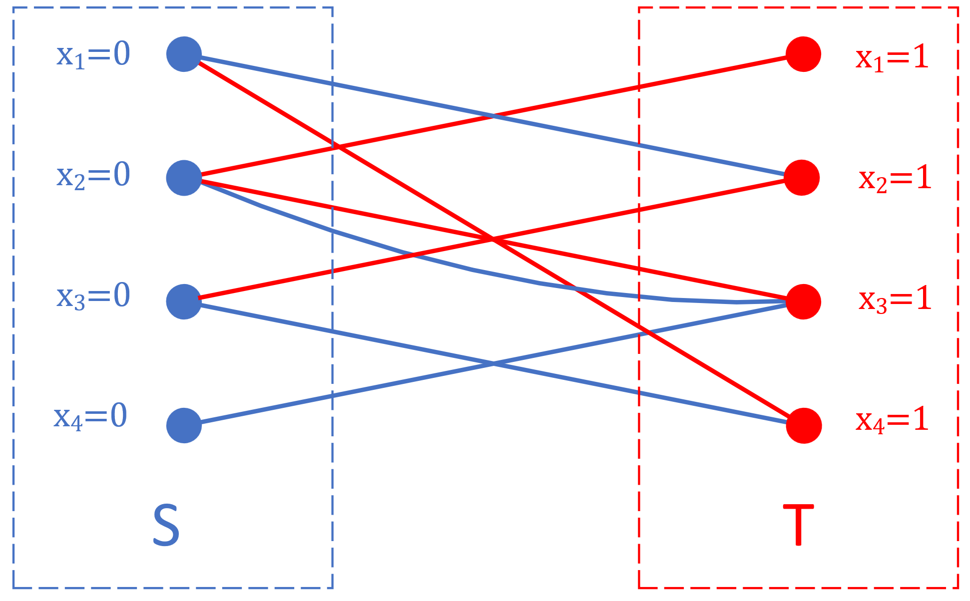
Figure 2: An example of $G_{X}$. Blue edges refer to directed edges in $B$, heading from $S$ to $T$. Red edges refer to directed edges in $R$, heading from $T$ to $S$.

With the two property, we again introduce an polynomial time approach to transform $\#\textsf{EO}(\mathcal{F})$ to a $\#\textsf{CSP}$ problem, where $\mathcal{F}$ contains only 0-rebalancing signatures.

Lemma 6.9.

Suppose $\mathcal{F}$ is composed of 0-rebalancing signatures. Then for any instance $\Omega(G(U,V,E),\pi)$ of $\textsf{Holant}(\neq_{2}\mid\mathcal{F})$, in polynomial time we can obtain another instance $\Omega^{\prime}(G(U,V,E),\pi^{\prime})$ of $\textsf{Holant}(\neq_{2}\mid\mathcal{F}^{\prime})$ such that $\textsf{Holant}_{\Omega^{\prime}}=\textsf{Holant}_{\Omega}$ , where $\mathcal{F}^{\prime}=\{f|_{\textsf{EO}^{P}}\mid f\in\mathcal{F},\text{ P is a pairing of Var}(f)\}$.

Proof 6.10.

Given an instance $I$ of $\textsf{Holant}(\neq_{2}\mid\mathcal{F})$ with $n$ signatures, let $s\in V$ assigned $f\in\mathcal{F}$ be an arbitrary vertex. By Lemma 6.7, $f$ is 0-rebalancing and $\hat{f}$ is 1-rebalancing. We use $\psi$ to denote the first level mapping of $f$ and $\theta$ to to denote the first level mapping of $\hat{f}$, and both mappings are associated with $E(s)=X=\{x_{1},x_{2},\cdots,x_{2d}\}$.

We use $G_{X}=(S,T,B\cup R)$ to denote the directed bipartite graph defined by $X,\psi$ and $\theta$ where $S=\{s_{i}\mid 1\leq i\leq 2d\},T=\{t_{j}\mid 1\leq j\leq 2d\},B=\{s_{i}t_{j}\mid 1\leq i\leq 2d,1\leq j\leq 2d,\psi(x_{i})=x_{j}\}$ and $R=\{t_{j}s_{i}\mid 1\leq i\leq 2d,1\leq j\leq 2d,\theta(x_{j})=x_{i}\}$. See Figure 2 for an example.

We remark that for each $x_{i}\in X$, $s_{i}$ and $t_{i}$ represent the statements $[x_{i}=0]$ and $[x_{i}=1]$ respectively. Each directed edge $s_{i}t_{j}$ represents that the statement $[x_{i}=0\to x_{j}=1]$ is always True. We write $x_{i}=0\to x_{j}=1$ for short. This is guaranteed by the 0-rebalancing property. Similarly, each directed edge $t_{j}s_{i}$ represents that $x_{j}=1\to x_{i}=0$.

As $\psi$ and $\theta$ are two mappings on $X$, the out-degree of each vertex in $S\cup T$ is exactly one. Consequently, there exists a directed cycle, namely $s_{i}t_{j}s_{k}\cdots s_{i}$.

If $x_{i}=0$, by the edge $s_{i}t_{j}$ we have $x_{j}=1$. If $x_{j}=1$, by the path $t_{j}s_{k}\cdots s_{i}$ we have $x_{i}=0$. Consequently, $x_{i}$ and $x_{j}$ can not take the same value in the instance. Let $x_{i}=p,x_{j}=q$. We add the pair $(p,q)$ to the pairing $P_{s}$ and replace $f$ and $\hat{f}$ with $f|_{p\neq q}$ and $\hat{f}|_{p\neq q}$.

After this, we update $\psi$ to $\psi^{\prime}$ in the following way:

$$\psi^{\prime}(x)=\left\{\begin{array}[]{ll}q&\text{ if }x=p;\\ p&\text{ if }x=q;\\ \psi(x)&\text{ if }x\neq p,q,\psi(x)\in X;\\ \psi_{2}^{x=0,p=1}(q)&\text{ if }x\neq p,q,\psi(x)=p;\\ \psi_{2}^{x=0,q=1}(p)&\text{ if }x\neq p,q,\psi(x)=q.\end{array}\right.$$

Similar to the proof of Lemma 6.3, $\psi^{\prime}$ can also be a witness for the 0-rebalancing property of the signature $f|_{p\neq q}$. We also update $\theta$ to $\theta^{\prime}$ similarly.

Now consider the directed bipartite graph $G_{X}^{\prime}$ defined by $X,\psi^{\prime}$ and $\theta^{\prime}$. We can see that $s_{i}t_{j},s_{j}t_{i},t_{i}s_{j},t_{j}s_{i}\in G_{X}^{\prime}$, forming two isolated connecting components. Consequently we may ignore them and apply the analysis above to $G_{X}^{\prime}-s_{i},s_{j},t_{i},t_{j}$ to obtain another opposite pair of variables, which means this process can be done successively. At the end of the procedure, we obtain $P_{v}$ which is the desired pairing that restrict $f$.

At the beginning of the algorithm, $\theta$ can be computed in $O(2d\cdot n)$ time, by using the 0-rebalancing property successively on the gadget $G-s$ to compute a tour from each variable of $s$ to another variable of it. After that, finding a directed loop in $G_{X}$ and updating $\psi$ need $poly(d)$ time, which is a constant. Updating $\theta$, however, needs $O(n)$ time. Each vertex $s$ need $d$ steps to clarify $P_{s}$, and there are $n$ vertices in total. Consequently, the time complexity of the algorithm is $O(n^{2})$, which is polynomial.

Along with Theorem 2.8 and Lemma 2.4, we present the algorithm in Theorem 3.6.

Proof 6.11 (Proof of tractability).

Given an instance of $\textsf{Holant}(\neq_{2}\mid\mathcal{F})$, by Lemma 6.9 we can transform it to a instance of $\textsf{Holant}(\neq_{2}\mid\mathcal{F}^{\prime})$ in polynomial time, where $\mathcal{F}^{\prime}=\{f|_{\textsf{EO}^{P}}\mid f\in\mathcal{F},\text{ P is a pairing of Var}(f)\}$. By Definition 3.3, $\mathcal{F}^{\prime}\subseteq\mathscr{A}$ or $\mathcal{F}^{\prime}\subseteq\mathscr{P}$. Then by Lemma 2.4 and the polynomial time algorithms in Theorem 2.8 for $\#\textsf{CSP}$ problems, the partition function of the latter instance can be calculated in polynomial time.

7 Conclusion

We proved two dichotomies for $\#\textsf{EO}(\mathcal{F})$ with $\mathcal{F}$ in specific cases, namely the case where $\mathcal{F}$ is restricted to a set of binary and quaternary signatures and the case where $\mathcal{F}$ contains only pure signatures respectively. It is worth studying to seek for a complete dichotomy for $\#\textsf{EO}$ problems.

In particular, the signature $f_{56}$ defined in Section 3.1, is not pure or rebalancing. The complexity of $\#\textsf{EO}(\{f_{56}\})$ remains unknown and is of our interest. Some progress has been made in this problem, but the authors are still facing non-trivial obstacles. In a related paper to be submitted, we give a $\textbf{P}^{\textbf{NP}}$ algorithm for #EO$(f_{56})$. Moreover, a complete dichotomy based on $\textbf{P}^{\textbf{NP}}\neq\#\textbf{P}$ for $\#\textsf{EO}$ problems is presented in that paper. However, whether $\#\textsf{EO}(f_{56})$ can be computed in polynomial time remains unsettled.

References

- [1] Miriam Backens. A complete dichotomy for complex-valued . arXiv preprint arXiv:1704.05798, 2017.
- [2] Miriam Backens. A new Holant dichotomy inspired by quantum computation. arXiv preprint arXiv:1702.00767, 2017.
- [3] David M Bressoud. Proofs and confirmations: the story of the alternating-sign matrix conjecture. Cambridge University Press, 1999.
- [4] Andrei Bulatov, Martin Dyer, Leslie Ann Goldberg, Markus Jalsenius, Mark Jerrum, and David Richerby. The complexity of weighted and unweighted #CSP. Journal of Computer and System Sciences, 78(2):681–688, 2012.
- [5] Andrei Bulatov, Martin Dyer, Leslie Ann Goldberg, Markus Jalsenius, and David Richerby. The complexity of weighted Boolean #CSP with mixed signs. Theoretical Computer Science, 410(38-40):3949–3961, 2009.
- [6] Andrei Bulatov and Martin Grohe. The complexity of partition functions. Theoretical Computer Science, 348(2-3):148–186, 2005.
- [7] Andrei A Bulatov. The complexity of the counting constraint satisfaction problem. Journal of the ACM (JACM), 60(5):1–41, 2013.
- [8] Andrei A Bulatov and Víctor Dalmau. Towards a dichotomy theorem for the counting constraint satisfaction problem. Information and Computation, 205(5):651–678, 2007.
- [9] Jin-Yi Cai and Xi Chen. Complexity dichotomies for counting problems: Volume 1, Boolean domain. Cambridge University Press, 2017.
- [10] Jin-Yi Cai and Xi Chen. Complexity of counting CSP with complex weights. Journal of the ACM (JACM), 64(3):1–39, 2017.
- [11] Jin-Yi Cai and Xi Chen. A decidable dichotomy theorem on directed graph homomorphisms with non-negative weights. computational complexity, 28:345–408, 2019.
- [12] Jin-Yi Cai, Xi Chen, and Pinyan Lu. Graph homomorphisms with complex values: A dichotomy theorem. SIAM Journal on Computing, 42(3):924–1029, 2013.
- [13] Jin-Yi Cai, Xi Chen, and Pinyan Lu. Nonnegative weighted #CSP: an effective complexity dichotomy. SIAM Journal on Computing, 45(6):2177–2198, 2016.
- [14] Jin-Yi Cai and Vinay Choudhary. Valiant’s Holant theorem and matchgate tensors. Theoretical Computer Science, 384(1):22–32, 2007.
- [15] Jin-Yi Cai, Zhiguo Fu, and Shuai Shao. Beyond #CSP: A dichotomy for counting weighted Eulerian orientations with ARS. Information and Computation, 275:104589, 2020.
- [16] Jin-Yi Cai, Zhiguo Fu, and Shuai Shao. From Holant to quantum entanglement and back. arXiv preprint arXiv:2004.05706, 2020.
- [17] Jin-Yi Cai, Zhiguo Fu, and Mingji Xia. Complexity classification of the six-vertex model. Information and Computation, 259:130–141, 2018.
- [18] Jin-Yi Cai and Artem Govorov. Perfect matchings, rank of connection tensors and graph homomorphisms. Combinatorics, Probability and Computing, 31(2):268–303, 2022.
- [19] Jin-Yi Cai, Heng Guo, and Tyson Williams. A complete dichotomy rises from the capture of vanishing signatures. In Proceedings of the forty-fifth annual ACM symposium on Theory of computing, pages 635–644, 2013.
- [20] Jin-Yi Cai, Pinyan Lu, and Mingji Xia. Holant problems and counting CSP. In Proceedings of the forty-first annual ACM symposium on Theory of computing, pages 715–724, 2009.
- [21] Jin-Yi Cai, Pinyan Lu, and Mingji Xia. Computational complexity of Holant problems. SIAM Journal on Computing, 40(4):1101–1132, 2011.
- [22] Jin-Yi Cai, Pinyan Lu, and Mingji Xia. Dichotomy for Holant* problems of Boolean domain. In Proceedings of the twenty-second annual ACM-SIAM symposium on Discrete Algorithms, pages 1714–1728. SIAM, 2011.
- [23] Jin-Yi Cai, Pinyan Lu, and Mingji Xia. The complexity of complex weighted Boolean #CSP. Journal of Computer and System Sciences, 80(1):217–236, 2014.
- [24] Jin-Yi Cai, Pinyan Lu, and Mingji Xia. Dichotomy for real problems. In Proceedings of the Twenty-Ninth Annual ACM-SIAM Symposium on Discrete Algorithms, pages 1802–1821. SIAM, 2018.
- [25] Martin Dyer, Leslie Ann Goldberg, and Mark Jerrum. The complexity of weighted Boolean #CSP. SIAM Journal on Computing, 38(5):1970–1986, 2009.
- [26] Martin Dyer, Leslie Ann Goldberg, and Mike Paterson. On counting homomorphisms to directed acyclic graphs. Journal of the ACM (JACM), 54(6):27–es, 2007.
- [27] Martin Dyer and Catherine Greenhill. The complexity of counting graph homomorphisms. Random Structures & Algorithms, 17(3-4):260–289, 2000.
- [28] Martin Dyer and David Richerby. An effective dichotomy for the counting constraint satisfaction problem. SIAM Journal on Computing, 42(3):1245–1274, 2013.
- [29] Martin E Dyer and David M Richerby. On the complexity of #CSP. In Proceedings of the forty-second ACM symposium on Theory of computing, pages 725–734, 2010.
- [30] Leslie Ann Goldberg, Martin Grohe, Mark Jerrum, and Marc Thurley. A complexity dichotomy for partition functions with mixed signs. SIAM Journal on Computing, 39(7):3336–3402, 2010.
- [31] Heng Guo, Sangxia Huang, Pinyan Lu, and Mingji Xia. The complexity of weighted Boolean #CSP modulo k. In STACS 2011, pages 249–260. Schloss Dagstuhl-Leibniz-Zentrum fuer Informatik, 2011.
- [32] Pavol Hell and Jaroslav Nešetřil. On the complexity of H-coloring. Journal of Combinatorial Theory, Series B, 48(1):92–110, 1990.
- [33] Michel Las Vergnas. On the evaluation at (3, 3) of the Tutte polynomial of a graph. Journal of Combinatorial Theory, Series B, 45(3):367–372, 1988.
- [34] Jiabao Lin and Hanpin Wang. The complexity of Boolean Holant problems with nonnegative weights. SIAM Journal on Computing, 47(3):798–828, 2018.
- [35] László Lovász. Operations with structures. Acta Mathematica Hungarica, 18(3-4):321–328, 1967.
- [36] Linus Pauling. The structure and entropy of ice and of other crystals with some randomness of atomic arrangement. Journal of the American Chemical Society, 57(12):2680–2684, 1935.
- [37] Shuai Shao and Jin-Yi Cai. A dichotomy for real Boolean Holant problems. In 2020 IEEE 61st Annual Symposium on Foundations of Computer Science (FOCS), pages 1091–1102. IEEE, 2020.
- [38] Leslie G Valiant. Holographic algorithms. SIAM Journal on Computing, 37(5):1565–1594, 2008.