Hyperbolic Random Graphs: Clique Number and Degeneracy with Implications for Colouring

Abstract

Hyperbolic random graphs inherit many properties that are present in real-world networks. The hyperbolic geometry imposes a scale-free network with a strong clustering coefficient. Other properties like a giant component, the small world phenomena and others follow. This motivates the design of simple algorithms for hyperbolic random graphs.

In this paper we consider threshold hyperbolic random graphs (HRGs). Greedy heuristics are commonly used in practice as they deliver a good approximations to the optimal solution even though their theoretical analysis would suggest otherwise. A typical example for HRGs are degeneracy-based greedy algorithms [Bläsius, Fischbeck; Transactions of Algorithms ’24]. In an attempt to bridge this theory-practice gap we characterise the parameter of degeneracy yielding a simple approximation algorithm for colouring HRGs. The approximation ratio of our algorithm ranges from $(2/\sqrt{3})$ to $4/3$ depending on the power-law exponent of the model. We complement our findings for the degeneracy with new insights on the clique number of hyperbolic random graphs. We show that degeneracy and clique number are substantially different and derive an improved upper bound on the clique number. Additionally, we show that the core of HRGs does not constitute the largest clique.

Lastly we demonstrate that the degeneracy of the closely related standard model of geometric inhomogeneous random graphs behaves inherently different compared to the one of hyperbolic random graphs.

1 Introduction

Many real-world networks have a heterogeneous degree distribution, close to a power-law, as well as a constant clustering coefficient. The hyperbolic random graph model (HRG) introduced by Krioukov et. al. [27] combines both properties [18], which has led to considerable interest in recent year. Various aspects of HRGs have been studied, including clique size [7, 8, 15], treewidth [9], minimum vertex cover size [3, 4], and diameter [16, 23, 31]. A hyperbolic random graph is a graph embedded in the hyperbolic plane where pairs of vertices have an edge if they are close according to the hyperbolic distance. It is generated by randomly throwing $n$ vertices on a disk of radius $R$ (dependent on $n$). Since hyperbolic space grows exponentially, most vertices are of small degree and located close to the boundary of the disk, while few vertices have large degree and lie close to the centre. This distribution of vertices leads to the power-law degree distribution of HRGs.

In this paper, we study the vertex colouring problem on HRGs, along with the related concepts of clique number and degeneracy. The $k$-colouring problem asks to colour the vertices of a graph with $k$ colours, while assigning different colours to adjacent vertices. The chromatic number $\chi(G)$ is the minimum number of colours needed to colour a graph in such a way. For $k\geq 3$ the problem is one of the original NP-hard problems [12, 20]. On general graphs, even loosely approximating the chromatic number is particularly hard [34].

The answer to the colouring problem is closely related to the clique number $\omega(G)$ and the degeneracy of a graph. The clique number is the number of vertices of the largest clique of the graph and it serves as a natural lower bound to the chromatic number. The degeneracy $\kappa(G)$ is the minimum integer $k^{\prime}$ for which there exists an ordering of the vertex set of $G$, $V=(v_{1},v_{2},\cdots,v_{n})$, such that for every index $i\in[n-1]$, $v_{i}$ has at most $k^{\prime}$ neighbours with greater index. Any graph $G$ can be easily coloured with $\kappa(G)+1$ colours by iterating through the vertices in reverse order and simply colouring a vertex with a colour not used by any of its higher ranked neighbours.

We aim to study these structural parameters that are not only fundamental to the model but also in general for algorithm design in various models of computation [1, 11, 17]. The most prominent large clique in an HRG is formed by the vertices in the graph’s core [7]. Simply put, the core emerges among the polynomially many vertices of distance at most $R/2$ from the centre of the disk, which due to the triangle inequality form a clique. At this point one may wonder whether the core forms the largest clique of the graph, a statement that we disprove in Proposition 4.7. Nevertheless we show that the largest clique can at most be a small constant factor larger than the core.

Theorem (Informal version of Theorem 4.10).

There exists a constant $\delta>0$ such that for any threshold HRG $G$, $\sigma(G)+1\leq\omega(G)\leq\sqrt{2-\delta}\cdot\sigma(G)$ holds w.e.h.p.

This upper bound improves on prior work [7], which showed that there exists some constant $c>1$ such that $\omega(G)\leq c\cdot\sigma(G)$ holds w.e.h.p., but without providing any upper bound on $c$.

We can now see that the core and clique are not the same. Nonetheless, (i) this theorem shows that the largest clique size and the core size are closely related, and (ii) the core of HRGs is a very well understood object, whereas the largest clique is not. Thus the natural next step is to bound the degeneracy using the core. We show the following theorem.

Theorem (Informal version of Theorems 3.5 and 3.5).

There exists constants $\delta_{1},\delta_{2}>0$ such that for any threshold HRG $G$, $(1+\delta_{1})\sigma(G)\leq\kappa(G)\leq(2-\delta_{2})\cdot\sigma(G)$ holds w.e.h.p.

The main surprise of this theorem is that the degeneracy is bounded away from the coresize by a constant factor. As the chromatic number is lower bounded by the core size, the upper bound on the degeneracy in this theorem implies a simple algorithm colouring with at most $(2-\delta_{2})\chi(G)$ colours. The approximation guarantee of this algorithm ranges from $2/\sqrt{3}$ to $4/3$ depending on further model parameters, see Section 2 and Theorem 3.8 for details. In any case, this improves on the previously best approximation ratio of $2$ [6, Lemma 7]. As discussed earlier this algorithm iteratively removes vertices of degree at most $(2-\delta_{2})\sigma(G)-1$ and then colours them in the reverse order. The next thing one would hope is to be able colour the graph with $\omega(G)$ colours using the same process. In [2], the authors conducted experiments where they were iteratively removing the vertex with the smallest degree of the graph, up to vertices with residual degree equal to the $\omega(G)$. In their findings, this process did not remove every vertex, implying $\omega(G)$ < $\kappa(G)$ for their generated graphs. We substantiate their findings by providing a rigorous proof demonstrating that the clique number is, in fact, a constant factor smaller than the degeneracy.

Theorem (Informal version of Theorem 4.3).

There exists a constant $\varepsilon>0$ such that for any threshold HRG $G$, $\omega(G)\leq(1-\varepsilon)\cdot\kappa(G)$ holds w.e.h.p.

Our final contribution is to study the degeneracy of geometric inhomogeneous random graphs (GIRGs) [22], a sibling to HRGs. The GIRGs also combine heterogeneity and high clustering. For most properties GIRGs and HRGs exhibit the same behavior. Perhaps the first paper to find a difference between them is [8], where the authors show that the minimum number of maximal cliques in the two models is not the same. We show that the degeneracy between HRGs and GIRGs is signifcantly different, see Figure 1 and Corollary 5.5.

Outline. See Figure 1 for a table with our results, as well as a plot comparing the bounds of our theorems for various model parameters. In Section 1.1 we provide a detailed discussion of our results and techniques. Section 3 contains bounds on the degeneracy of HRGs (Theorem 3.5). In Section 4, we show the gap between clique number and degeneracy (Theorem 4.3), as well as bounds on the clique number (Theorem 4.10). Finally, Section 5 contains results about the degeneracy of GIRGs. Statements where proofs or details are omitted due to space constraints can be found in the provided appendix.

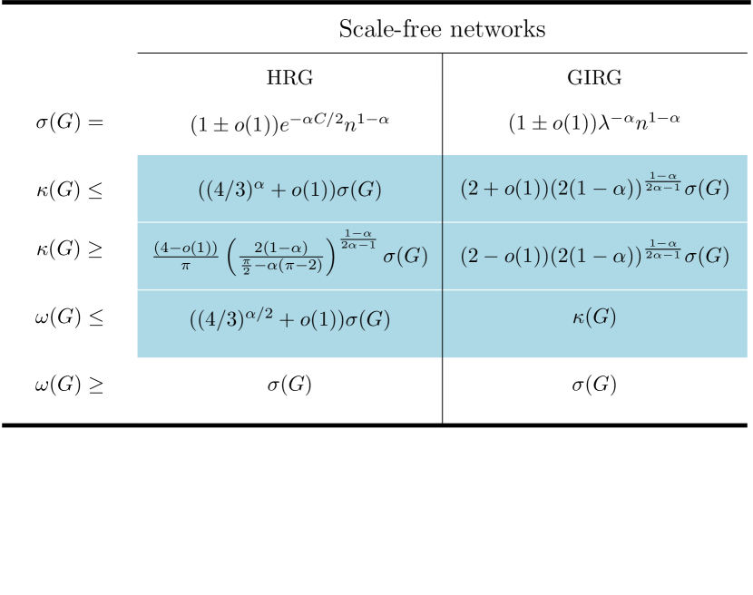
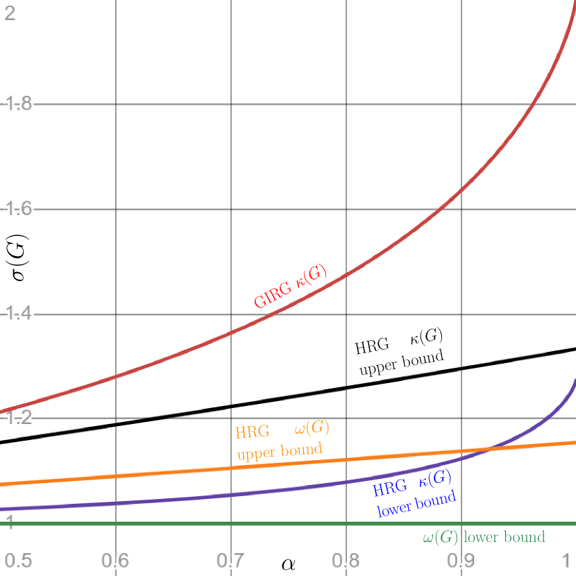
Figure 1: Results on the degeneracy $\kappa(G)$ and the size of the largest clique $\omega(G)$ in hyperbolic random graphs (HRG) and geometric inhomogeneous random graphs (GIRG). The bounds hold w.e.h.p. and are stated in comparison to the core size $\sigma(G)$. The dependency on the model parameter $\alpha\in(1/2,1)$ is plotted on the x-axis with respect to the multiplicative factor in front of the core size $\sigma(G)$ on the y-axis. Prior work is listed with white background, whereas our results are listed with blue background.

1.1 Discussion of our Results and Techniques

As discussed HRGs have a power-law degree distribution [18, 32], that is, the probability that a vertex has degree $k$ is given by $\sim k^{-(2\alpha+1)}$ . The model parameter $\alpha\in(1/2,1)$ controls the power-law exponent and all our results, particularly the size of the aforementioned constant factor gap depends on the choice of $\alpha$. For the easy of presentation this overview largely omits this dependence, but the summary of our results in Figure 1 plots it in detail.

Upper bound on degeneracy (Theorem 3.5). One consequence of generating a graph in hyperbolic space is that vertices tend to have fewer neighbours with increasing radius, i.e., the expected number of neighbours of a vertex decreases with the distance from the centre of the hyperbolic disc. This produces the power-law degree distribution that is valuable in modelling real-world networks. It also leads to a simple approach for upper bounding degeneracy: instead of removing vertices ordered by (increasing) degree, we remove them by (decreasing) radius. If $k$ is such that each vertex has at most $k$ neighbours of smaller radius, then $k$ is an upper bound on the degeneracy.

The notion governing this approach is the inner-neighbourhood of a vertex, see Figure 2. The inner-neighbourhood of a vertex $u$ with radius $r$, denoted $\operatorname{\Gamma}(u)$, is the set of vertices of distance at most $R$ from $u$, i.e., they are neighbours of $u$, and with radius at most $r$, i.e., they are closer to the centre of the disc than $u$. The size $|\operatorname{\Gamma}(u)|$ of the inner-neighbourhood is called the inner-degree of $u$. The expected value of $|\operatorname{\Gamma}(u)|$ scales with the area of $u$’s inner-ball $\mathcal{I}(r)=\mathcal{B}_{u}(R)\cap\mathcal{B}_{0}(r)$. More precisely, $\mathbb{E}\left[|\operatorname{\Gamma}(u)|\right]=(n-1)\cdot\mu(\mathcal{I}(r))$. See Figure 2 a for a visual representation. The vertex of largest inner-degree is denoted $u^{*}$; the choice of $u^{*}$ and the value of $|\operatorname{\Gamma}(u^{*})|$ depend on the random distribution of the vertices.

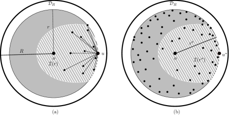
Figure 2: Illustration of the inner-neighbourhood. (a) The grey area is the ball $\mathcal{B}_{0}(r)$. The hatched area $\mathcal{I}(r)=\mathcal{B}_{u}(R)\cap\mathcal{B}_{0}(r)$ is the inner-ball of $u$. The vertices in $\mathcal{I}(r)$ form the inner-neighbourhood of $u$. (b) Sketch of proof of Lemma 3.2. Vertex $u^{*}$ is the vertex with the largest inner-degree. Each vertex $v\in U=V\cap\mathcal{B}_{0}(r^{*})$ has at least nearly as many neighbours within $\mathcal{B}_{0}(r^{*})$ as $|\operatorname{\Gamma}(u^{*})|$ (w.e.h.p.)

If vertices are removed from outside to inside, then each vertex at the time of its removal will have degree less or equal to the inner-degree of $u^{*}$. To bound the degeneracy, we derive a probabilistic upper bound for $|\operatorname{\Gamma}(u^{*})|$. We do this by finding the radius that maximises $\mu(\mathcal{I}(r))$, which upper bounds $\mathbb{E}\left[|\operatorname{\Gamma}(u)|\right]$ (for every vertex $u$). Since $|\operatorname{\Gamma}(u)|$ is concentrated we can apply a Chernoff and a union bound to obtain a high probability upper bound for $|\operatorname{\Gamma}(u^{*})|$. Despite the simplicity of the inner-neighbourhood, we elaborate on this key concept as it is not only crucial to our upper bound on degeneracy but also for most of our other results discussed later on.

Lower bound on degeneracy (Theorem 3.5). Surprisingly, we show in Lemma 3.2 that the maximum inner-degree also produces a lower bound on the degeneracy $\kappa(G)$, in the sense that $\kappa(G)\geq(1-o(1))|\operatorname{\Gamma}(u^{*})|$ w.e.h.p. This yields asymptotically tight bounds on $\kappa(G)$. We prove the lower bound of $\kappa(G)$ by considering the subgraph $G^{\prime}$ induced by the vertices that have smaller radius than $u^{*}$ (see Figure 2 b). Note that $G^{\prime}$ contains vertices that are not neighbours of $u^{*}$. We show that every vertex $u$ in $G^{\prime}$ has, w.e.h.p., at least $(1-o(1))|\operatorname{\Gamma}(u^{*})|$ neighbours in $G^{\prime}$; this statement uses the choice of $u^{*}$ and is not true if $u$ was an arbitrary vertex of the graph. Now, in any ordering of the vertices of $G^{\prime}$, the first vertex has at least $(1-o(1))|\operatorname{\Gamma}(u^{*})|$ neighbours of greater index, implying $(1-o(1))|\operatorname{\Gamma}(u^{*})|\leq\kappa(G^{\prime})\leq\kappa(G)$. While this provides a lower bound that asymptotically matches our upper bound, a lower order gap remains.

Gap between clique number and degeneracy (Theorem 4.3). The most immediate lower bound for degeneracy is the clique number [1], because in every ordering of the vertices of $G$, the vertex of the clique with the lowest index has at least $\omega(G)-1$ neighbours of higher index. We prove that the lower bounds on the degeneracy that are derived from the clique number are strictly worse than the bounds discussed above obtained via analysing the inner-degree. Our approach to show this is the following: we take an arbitrary clique $K$ and the vertex $u$ with the largest radius in $K$. Let $G^{\prime\prime}$ be the subgraph induced by $\operatorname{\Gamma}(u)$. Next, we partition $G^{\prime\prime}$ intro three sets of vertices, each containing at least a constant fraction of the vertices of $G^{\prime\prime}$ w.e.h.p. See Figure 3 b for an illustration of this partition. Lastly, we use purely geometric arguments to show that $K$ cannot contain vertices from all three sets. As the left out set contains a constant fraction of $u$’s inner neighbourhood, implying the gap. This gap between $\omega(G)$ and $\kappa(G)$ and makes approaches for computing the clique number via degeneracy, like that of Walteros and Buchanan [33], unsuitable for HRGs.

Clique number and the core (Theorem 4.10). The upper bound on the clique number is proven via a geometric approach. Let $u,v,w$ be any three vertices. If the vertices are far apart they cannot be contained in a clique. Otherwise their pairwise distance is at most $R$. Using the hyperbolic version Jung’s theorem [19, 13, 14] implies that they are contained in a ball $\mathcal{B}$ of small radius and we show that $\mathcal{B}$ also has a small area. Hence the expected number of vertices in $\mathcal{B}$ is small as well. As this expectation is well concentrated whenever the area is significantly large, this bound holds with extremely high probability when introducing lower order deviations from the expectation. Via a union bound over all possible $\binom{n}{3}$ triples of vertices we rule out that any clique contained in such a covering ball is large. The main claim now follows because any clique has to be contained in one of these coverings balls.

The question of whether $\omega(G)/\sigma(G)\to 1$ as $n\to\infty$ remains open.

2 Preliminaries

Hyperbolic Random Graphs.

We follow the formalisation of hyperbolic random graphs introduced in [32], which is known as the native representation. We denote by $\mathbb{H}^{2}=[0,\infty)\times[0,2\pi)$ the hyperbolic plane in the polar coordinate system, where points $x\in\mathbb{H}^{2}$ is parameterised by a radius $r(x)$ and an angle $\varphi(x)$. We equip $\mathbb{H}^{2}$ with a metric $\operatorname{d_{h}}(x,y)$ characterised by

$$\cosh(\operatorname{d_{h}}(x,y))=\cosh(r(x))\cosh(r(y))-\sinh(r(y))\sinh(r(x))\cos(\varphi(x)-\varphi(y)).$$ (1)

This metric is what gives $\mathbb{H}^{2}$ a hyperbolic geometry, of curvature -1, as opposed to the Euclidean metric. We equip $\mathbb{H}^{2}$ with the topology induced by $\operatorname{d_{h}}$.

The geometric space of most importance in this work is the bounded disk in $\mathbb{H}^{2}$ defined by $\mathcal{D}_{R}=[0,R]\times[0,2\pi)$, where $R=2\log(n)+C$ with $C\in\Theta(1)$. We refer to point $(0,0)$ as the centre of this disk. The space $\mathcal{D}_{R}$ inherits the topology of $\mathbb{H}^{2}$, and from now on we shall only consider subsets of this space – thus, for example, a ball around a point $y\in\mathcal{D}_{R}$ is defined by the set $\mathcal{B}_{\varepsilon}(y)=\{x\in\mathcal{D}_{R}:\operatorname{d_{h}}(x,y)\leq\varepsilon\}\subseteq\mathcal{D}_{R}$.

We now introduce a probability measure $\mu$ on $\mathcal{D}_{R}$, which is parametrised by the model parameter $\alpha\in(1/2,1)$, and was first defined by Papadopoulos et. al. [32]. For measurable $\mathcal{S}\subseteq\mathcal{D}_{R}$, define

$$\mu(\mathcal{S})=\int_{S}\rho(x)\,\mathrm{d}x,\qquad\rho(x)=\frac{\alpha\sinh(\alpha x)}{2\pi(\cosh(\alpha R)-1)},$$

where $\mathrm{d}x$ denotes the Lebesgue measure on $\mathcal{D}_{R}$. This measure differs from the uniform probability measure on $\mathcal{D}_{R}$ in that it puts more mass at the centre of the disk; both measures coincide at $\alpha=1$. The benefit of $\mu$ lies in the properties it induces in our central object of study, the hyperbolic random graph.

Threshold hyperbolic random graph (HRG).

A (threshold) hyperbolic random graph or HRG is a pair $G=(V,E)$ defined by the following procedure. First, $n$ vertices are sampled independently at random in $\mathcal{D}_{R}$ according to $\mu$. Then any two vertices $u,v\in V$ are connected by an edge if and only if their distance $\operatorname{d_{h}}(u,v)$ is at most $R$. We write $G\sim\mathcal{G}(n,\alpha,C)$ to denote a graph generated in this way.

The use of $\mu$ to distribute vertices in $\mathcal{D}_{R}$ has the effect of giving $G$ a power-law degree distribution, as was shown in [18, 32]. It is sometimes convenient to characterise connection of vertices in terms of their angular distance, and to that end we define

$$\theta_{R}(r_{1},r_{2})=\arccos\left(\frac{\cosh(r_{1})\cosh(r_{2})-\cosh(R)}{\sinh(r_{1}\sinh(r_{2})}\right),$$

which per (1) yields the following observation. Two vertices $u$ and $v$ are connected if and only if their angular distance is less than $\theta_{R}(r(u),r(v))$. We also make use of the following expression of the distribution of the radius of a vertex $u$.

$$\mathbb{P}\left(r(u)\leq r\right)=\mu\left(\mathcal{B}_{0}(r)\right)=\int_{0}^{r}\int_{-\pi}^{\pi}\rho(x)\,\mathrm{d}\theta\,\mathrm{d}x=\frac{\cosh(\alpha r)-1}{\cosh(\alpha R)-1}=(1-o(1))e^{-\alpha(R-r)}$$ (2)

We briefly note that a variant of HRGs exists in which vertices are not connected purely according to whether their distance is below a threshold, but rather with probability $p(u,v)=(1+\exp\left(\frac{1}{2T}\left(\operatorname{d_{h}}(u,v)-R\right)\right))^{-1}$ determined by both distance and a “temperature” parameter $T$ (see e.g. [28, §3.1]).

Degeneracy, clique number, chromatic number and core. For a graph $G=(V,E)$, the degeneracy $\kappa(G)$ is the minimum integer $k$ for which there exists an ordering of the vertex set of $G$, $V=(v_{1},v_{2},\cdots,v_{n})$, such that for every index $i\in[n-1]$, $v_{i}$ has at most $k$ neighbours with greater index. The clique number $\omega(G)$ is the size of the largest clique of $G$. The chromatic number $\chi(G)$ is the smallest number of colours required so that a conflict-free vertex colouring is possible for $G$. The core of a hyperbolic random graph is the set of vertices with radius at most $R/2$. Since for any points $u,v\in\mathcal{B}_{0}(R/2)$ the distance is at most $\operatorname{d_{h}}(u,v)\leq R$, the core forms a clique. We denote the size of the core by $\sigma(G)$. Finally, we note that the following chain of inequalities holds: $\sigma(G)\leq\omega(G)\leq\chi(G)\leq\kappa(G)+1.$

3 Degeneracy of Hyperbolic Random Graphs

A tool we make use of several times is the inner-ball of a point $x\in\mathcal{D}_{R}$, defined by $\mathcal{I}(x)=\mathcal{B}_{x}(R)\cap\mathcal{B}_{0}(r(x))$. Since area of an inner-ball is invariant under angular rotation we also write $\mathcal{I}(r)$. The inner-ball of a vertex is the inner-ball of the point using the vertex’ coordinates. The inner-neighbourhood of a vertex $u$ is the set of vertices (excluding $u$) contained in its inner-ball, that is, the neighbours of $u$ that have a smaller radius than $u$ (see Figure 2 a), and is denoted $\operatorname{\Gamma}(u)$.

We upper bound the degeneracy $\kappa(G)$ via the inner-neighbourhood by using the following informal process. Consider a graph $G$ and order its vertices $(v_{1},v_{2},\cdots,v_{n})$ by decreasing radius, so $r(v_{i})\geq r(v_{i+1})$, and iteratively remove vertices from $G$ one-by-one, from lower to higher index. Note that the set of neighbours of $v_{i}$ that have greater index than $i$ coincide with $\operatorname{\Gamma}(v_{i})$. This implies that the degree of each vertex $v_{i}$ at the time of its removal is $|\operatorname{\Gamma}(v_{k})|$. Let $u^{*}$ be the vertex $v_{k}$ that maximises $|\operatorname{\Gamma}(v_{k})|$. As the largest degree among vertices in this ordering is given by $|\operatorname{\Gamma}(u^{*})|$, we get the following upper bound for the degeneracy.

Let $G\sim\mathcal{G}(n,\alpha,C)$ be a threshold HRG and let $u^{*}$ be the vertex of $G$ with the largest inner-degree in $G$. Then $\kappa(G)\leq|\operatorname{\Gamma}(u^{*})|$.

We will now show that the largest inner-degree does not only yield an immediate upper bound on the degeneracy, but also a lower bound. Informally, this lower bound follows from the following argument. Order the vertices of the graph in ascending order of their radius, that is, $(v_{1},v_{2},\ldots,v_{n})$ such that $r(v_{i})\geq r(v_{i+1})$. For $i\in[n]$, let $G_{i}=G\setminus\{v_{1},v_{2},\ldots,v_{i}\}$. Let $v_{k}$ be the node with the maximum inner neighbourhood in $G$. We show (with a probabilistic guarantee) that graph $G_{k}$ has minimum degree $(1-o(1))|\operatorname{\Gamma}(v_{k})|$. Before we make this formal, we introduce a slightly modified version of [18, Lemma 3.3], that implies the following: the closer a vertex is to the origin, the more neighbours it has in expectation. This can be proven via the fact that the angle $\theta_{R}(r,x)$ is monotonically decreasing in $x$.

Corollary 3.1.

Let $r,s,t\in[0,R)$ with $s<t$. Then $\mu(\mathcal{B}_{s}(R)\cap\mathcal{B}_{0}(r))\geq\mu(\mathcal{B}_{t}(R)\cap\mathcal{B}_{0}(r))$.

From Corollary 3.1 it follows that any vertex with radius at most $r$ has in expectation at least as many neighbours with radius up to $r$, as the expected inner-degree of a vertex with radius exactly $r$. In order to derive a high-probability bound on $|\operatorname{\Gamma}(u^{*})|$ it now suffices to show concentration around the expectation of all considered neighbourhoods.

Let $G\sim\mathcal{G}(n,\alpha,C)$ be a threshold HRG. Then, $\omega(G)\geq\sigma(G)$.

Since the size of every clique $K$ is upper bounded by the inner-degree of the vertex in $u\in K$ that has the largest radius, $\omega(G)$ is a lower bound for the maximum inner-degree. We can now lower bound the degeneracy $\kappa(G)$ based on the largest inner-degree. Note that, in contrast to the upper bound of Section 3, the lower bound is not deterministic.

Lemma 3.2.

Let $G\sim\mathcal{G}(n,\alpha,C)$ be a threshold HRG. Then $\kappa(G)\geq(1-o(1))|\operatorname{\Gamma}(u^{*})|$ w.e.h.p.

Proof 3.3.

For any subgraph $H\subseteq G$, it is clear that $\kappa(G)\geq\min_{v\in V(H)}\mathrm{deg}|_{H}(v)$, where $\mathrm{deg}|_{H}(v)=\sum_{w\in V\setminus\{v\}}\mathbb{I}\{w\leftrightarrow v,w\in V(H)\}$. We let $H$ be the (random) subgraph of $G$ created by restricting $G$ to vertices that land in $\mathcal{B}_{0}(r)$, that is, that have radius less or equal $r$, and keeping the same edges.

Then for any $v\in V$,

$$\mathbb{E}[\mathrm{deg}|_{H}(v);r(v)\leq r] =\sum_{w\in V\setminus\{v\}}\mathbb{P}(w\in\mathcal{B}_{0}(r)\cap\mathcal{B}_{r(v)}(R),r(v)\leq r)$$

$$\geq\sum_{w\in V\setminus\{v\}}\mathbb{P}(w\in\mathcal{B}_{0}(r)\cap\mathcal{B}_{r}(R),r(v)\leq r)$$ (Corollary 3.1)

$$=(n-1)\mu(\mathcal{B}_{0}(r)\cap\mathcal{B}_{r}(R))\mathbb{P}(r(v)\leq r).$$

Thus $\mathbb{E}[\mathrm{deg}|_{H}(v)\,|\,r(v)\leq r]\geq(n-1)\mu(\mathcal{B}_{0}(r)\cap\mathcal{B}_{r}(R))\eqqcolon\gamma$. Since $\mathrm{deg}|_{H}(v)$ is a sum of Bernoulli random variables that are all independent under $\mathbb{P}(\,\cdot\,|\,r(v)\leq r)$, a Chernoff bound gives that it is highly concentrated around $\gamma$. Thus

$$\mathbb{P}\Big{(}\min_{v\in V(H)}\mathrm{deg}|_{H}(v)<(1-o(1))\gamma\Big{)} =\mathbb{P}\Big{(}\bigcup_{v\in V}\{\mathrm{deg}|_{H}(v)<(1-o(1))\gamma,r(v)\leq r\}\Big{)}$$

$$\leq n\mathbb{P}(\mathrm{deg}|_{H}(v)<(1-o(1))\gamma,r(v)\leq r)$$

$$\leq n\mathbb{P}(\mathrm{deg}|_{H}(v)<(1-o(1))\gamma\,|\,r(v)\leq r)\leq n\mathrm{e}^{-o(1)/2\gamma}.$$

Taking $r$ to be the argmax of $\gamma$ yields $\gamma(r)\geq\mathbb{E}[\Gamma(u^{*})]$. By Section 3 and applying (2) at $R/2$ we have that $\gamma(r)\geq\mathbb{E}[\Gamma(u^{*})]\geq\mathbb{E}[\sigma(G)]\in n^{\Omega(1)}.$ Thus for any choice of $c$ there is a large enough $n$ such that

$$\mathbb{P}(\kappa(G)<(1-o(1))|\operatorname{\Gamma}(u^{*})|)\leq\mathbb{P}(\kappa(G)<(1-o(1))\gamma(r))\leq n^{1-c},$$

that is, $\kappa(G)\geq(1-o(1))|\operatorname{\Gamma}(u^{*})|$ w.e.h.p.

In the rest of this section we derive bounds for the largest inner-degree on HRGs that hold w.e.h.p. which, by Sections 3 and 3.2, translate into results for the degeneracy. A vertex $v$ belongs to the inner-neighbourhood of a vertex $u$, if and only if it resides in the inner-ball of $u$. As such, we can use the measure $\mu\left(\mathcal{I}(r)\right)$ of an inner-ball $\mathcal{I}_{u}$ to bound the maximum inner-degree of a graph. Since the measure of the inner-ball is invariant under rotation around the origin, we write $\mu\left(\mathcal{I}(r)\right)$ instead of $\mu\left(\mathcal{I}_{u}\right)$ for $r=r(u)$. We sum up our results for the area of the inner-ball in the following lemma which is obtained by combining Lemmas C.1 and C.3 (see Appendix C) where explicit values for $\gamma$ and $\eta$ are also stated.

Lemma 3.4 (Volume of the inner-ball).

Let $\Delta\in\Theta(1)$ and let $u\in\mathcal{D}_{R}$ with radius $r=R/2+\Delta$. Then, depending on $\Delta$, there exist constants $\gamma,\eta$, such that

$$\mu(\mathcal{I}(r))=\left(1+\Theta\left(e^{-\alpha R}\right)\right)\frac{\alpha e^{-\alpha r}}{\alpha-1/2}\left(\gamma e^{\frac{1}{2}(2\alpha-1)(2r-R)}-\eta\right).$$

We use Lemma 3.4 to upper and lower bound the degeneracy. The lower bound tells us that there exists a constant $\delta_{\alpha}>0$ such that $\kappa(G)\geq(1+\delta_{\alpha})\sigma(G)$ w.e.h.p. The constant $\delta_{\alpha}$ is increasing with increasing $1/2<\alpha<1$, see Figure 1.

Theorem 3.5 (Bounds on degeneracy).

Let $G\sim\mathcal{G}(n,\alpha,C)$ be a threshold HRG. Then w.e.h.p. its degeneracy $\kappa(G)$ satisfies

$$\frac{(4-o(1))}{\pi}\left(\frac{2\left(1-\alpha\right)}{\frac{\pi}{2}-\alpha\left(\pi-2\right)}\right)^{\frac{1-\alpha}{2\alpha-1}}\sigma(G)\leq\kappa(G)\leq((4/3)^{\alpha}+o(1))\sigma(G).$$

Proof 3.6 (Proof sketch).

Differentiating $\mu(\mathcal{I}(r))$ we find $r^{*}$, which maximises it. The upper bound is obtained by using $r^{*}$ for the upper bound of the inner-ball with $(n-1)\mu(\mathcal{I}(r^{*}))$, and using a Chernoff bound along with a union bound which gives an upper bound for $|\operatorname{\Gamma}(u^{*})|$. Section 3 then yields the upper bound for the degeneracy. For the lower bound, we first show that there exists a vertex with a radius $\tilde{r}$ close in value to $r^{*}$. Then $(n-1)\mu(\mathcal{I}(\tilde{r}))$ lower bounds $|\operatorname{\Gamma}(u^{*})|$ w.e.h.p. This gives a lower bound for degeneracy, due to Lemma 3.2.

Recalling that $\omega(G)\leq\chi(G)\leq\kappa(G)+1$, and applying Sections 3 and 3.5, the following is immediate.

Corollary 3.7 (Bounds on chromatic number).

Let $G\sim\mathcal{G}(n,\alpha,C)$ be a threshold HRG. Then w.e.h.p. its chromatic number is $\sigma(G)\leq\chi(G)\leq((4/3)^{\alpha}+o(1))\sigma(G).$

Our structural results directly produce algorithmic applications. The small gap between degeneracy and core translates into an efficient approximation algorithm to colour a HRG.

Theorem 3.8.

Let $G\sim\mathcal{G}(n,\alpha,C)$ be a threshold HRG. Then an approximate vertex colouring of $G$ can be computed in time $\mathcal{O}(n)$ with approximation ratio $((4/3)^{\alpha}+o(1))$ w.e.h.p.

Proof 3.9 (Proof sketch.).

Using a smallest-last vertex ordering [29] the number of colours required is upper-bounded by $\kappa(G)$. The linear running time is a direct consequence of HRGs being sparse. The approximation ratio is achieved by comparing the lower bound of the chromatic number in Corollary 3.7 to the upper bound of the degeneracy in Theorem 3.5.

4 Clique Number of Hyperbolic Random Graphs

For any graph $G$, the clique number $\omega(G)$, chromatic number $\chi(G)$, and degeneracy $\kappa(G)$ are related via the inequalities $\omega(G)\leq\chi(G)\leq\kappa(G)+1$. If $G$ has $\kappa(G)=\omega(G)+1$, then $\chi(G)$ has the same value and can be computed in linear time. For this reason we are interested in the relationship between clique number and degeneracy for hyperbolic random graphs. In Section 4.1 we show that the two differ and that for HRGs, the degeneracy is strictly larger than the clique number by a constant multiplicative constant. In Section 4.2 we give new insights about where in the hyperbolic disk the largest clique is formed. We then conclude the section by providing a new upper bound for the clique number that states a leading constant in front of the size of the core, and that is increasing in $\alpha$.

4.1 The gap between Clique Number and Degeneracy

Because of the centralising effect of hyperbolic geometry, one might hope to show that the clique contained in the core of the disk is the largest, and that $\omega(G)=(1-o(1))\kappa(G)$. This would achieve two things: it would also imply a tight bound for the chromatic number $\chi(G)$, sandwiching it between clique number and degeneracy. It would also imply a linear time $(1+o(1))$-approximation algorithm for both clique number and chromatic number.

In this section we disprove these claims. We show that there exists a constant gap between clique number and degeneracy; this is the content of Theorem 4.3. Before embarking on the details of the proof, we first sketch its idea. For any clique $K$, its vertex $u$ with largest radius, whose inner-degree $|\operatorname{\Gamma}(u)|$ bounds $|K|$. For $r(u)\in R/2+o(1)$ and $r(u)\in R/2+\omega(1)$, $|\operatorname{\Gamma}(u)|$ is already smaller by a multiplicative constant than the lower bound for the degeneracy given in Theorem 3.5. What remains is to extend the result to $r(u)\in R/2+\Theta(1)$, which requires more intricate arguments and is addressed in the following lemma.

Lemma 4.1.

Let $G\sim\mathcal{G}(n,\alpha,C)$ be a threshold HRG, let $\Delta\in\Theta(1)$ be constant and let $K$ be a clique where $u\in K$ is the vertex with largest radius $r_{K}=R/2+\Delta$. Then w.e.h.p. there exists a constant $\varepsilon\in(0,1)$ such that $\omega(G)<(1-\varepsilon)\kappa(G)$.

Proof 4.2.

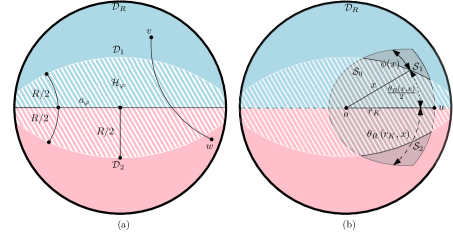
Figure 3: Illustration of a separator. (a) The line $a_{\varphi}$ partitions disk $\mathcal{D}_{R}$ into two halfdisks $\mathcal{D}_{1}$ (blue) and $\mathcal{D}_{2}$ (pink). The hypercycle $\mathcal{H}_{\varphi}$ (hatched area) is defined by the line $a_{\varphi}$. Points in located in different halfdisks and outside the hatched area have distance at least $R$. (b) The separator (hatched area) separates the inner-neighbourhood (grey area) of a vertex $u$ of radius $r_{K}$ into three sub-areas $\mathcal{S}_{0}$, $\mathcal{S}_{1}$ and $\mathcal{S}_{2}$. Any vertex located in $\mathcal{S}_{1}$ has no edge to a vertex in $\mathcal{S}_{2}$.

Let $G^{\prime}$ be the inner-neighbourhood of $u$, i.e., the induced subgraph $G^{\prime}=G[\Gamma(u_{K})]$. Then $K\subseteq V(G^{\prime})$, and thus $\omega(G^{\prime})\geq|K|$. We show that $\omega(G^{\prime})<(1-\varepsilon)|\operatorname{\Gamma}(u_{K})|$ w.e.h.p.

We accomplish this by proving that there exists a colouring for $G^{\prime}$ with $(1-\varepsilon)|V(G^{\prime})|=(1-\varepsilon)|\operatorname{\Gamma}(u_{K})|$ many colours. This implies an upper bound for the chromatic number $\chi(G^{\prime})$, which also serves as an upper bound for $\omega(G^{\prime})$. We do this by partitioning the inner-neighbourhood $\mathcal{I}\left(r_{K}\right)$ into three disjoint sub-regions $\mathcal{S}_{0}\cup\mathcal{S}_{1}\cup\mathcal{S}_{2}$ such that no vertex in $\mathcal{S}_{1}$ is adjacent to any vertex in $\mathcal{S}_{2}$. Thus, $\mathcal{S}_{0}$ separates $\mathcal{S}_{1}$ from $\mathcal{S}_{2}$ and we can colour the set of vertices $V\cap\mathcal{S}_{1}$ with the same colours as $V\cap\mathcal{S}_{2}$. Thus if $\min\{|V\cap\mathcal{S}_{1}|,|V\cap\mathcal{S}_{2}|\}\geq\varepsilon|\operatorname{\Gamma}(u)|$ w.e.h.p., our desired statement will be proven.

To find such a separator $\mathcal{S}_{0}$, we follow the lines drawn by Bläsius et. al. [9] where hypercycles for hyperbolic random graphs were introduced (see Figure 3 a). A hypercycle $\operatorname{\mathcal{H}}_{\varphi}$ (of radius $R/2$) is defined as follows: let $a_{\varphi}$ denote the line whose points have angle $\varphi$ and $\varphi+\pi$. Then $\operatorname{\mathcal{H}}_{\varphi}:=\{u\in\mathcal{D}_{R}:\operatorname{d_{h}}(u,a_{\varphi})\leq R/2\}$, i.e. the set of points with distance at most $R/2$ to line $a_{\varphi}$. Consider the point $u=\left(r_{K},\varphi\right)$ and let $\mathcal{S}_{0}:=\mathcal{I}_{u}\cap\operatorname{\mathcal{H}}_{\varphi}$. To define $\mathcal{S}_{1}$ and $\mathcal{S}_{2}$ separate $\mathcal{D}_{R}$ into the two disjoint halfdisks $\mathcal{D}_{1}=\{x\in\mathcal{D}_{R}:\varphi(x)-\varphi\leq\pi\}$ and $\mathcal{D}_{2}=\{x\in\mathcal{D}_{R}:\varphi(x)-\varphi\geq\pi\}$ (see Figure 3 a). Then we define $\mathcal{S}_{1}:=(\mathcal{I}_{u}\cap\mathcal{D}_{1})\setminus\operatorname{\mathcal{H}}_{\varphi}$ and symmetrically $\mathcal{S}_{2}:=(\mathcal{I}_{u}\cap\mathcal{D}_{2})\setminus\operatorname{\mathcal{H}}_{\varphi}$.

We observe that any point $w\in\mathcal{S}_{1}$ has distance at least $R$ to any point $v\in\mathcal{S}_{2}$. This can be shown for example by observing that the geodesic between $w$ and $v$ must pass through some point $x\in a_{\varphi}$, and so $\operatorname{d_{h}}(w,v)=\operatorname{d_{h}}(w,x)+\operatorname{d_{h}}(x,v)\geq\operatorname{d_{h}}(w,a_{\varphi})+\operatorname{d_{h}}(a_{\varphi},v)>R$. This ensures our objective of separating the two regions via $\mathcal{S}_{0}$.

Next, we show that there exists a constant $\varepsilon>0$ small enough, such that $\mu(\mathcal{S}_{1})=\mu(\mathcal{S}_{2})\geq\varepsilon n^{-\alpha}$ (a sketch of the idea is given in Figure 3 b). Setting $\phi(x)=\max(0,\theta_{R}\left(r_{K},x\right)-\theta_{R}(x,x)/2)$ we derive by symmetry

$$\mu(\mathcal{S}_{1})=\mu(\mathcal{S}_{2})=\int_{R/2}^{r}\int_{0}^{\phi(x)}\rho(x)\,\mathrm{d}\phi\,\mathrm{d}x=\int_{R/2}^{R/2+\Delta}\phi(x)\rho(x)\,\mathrm{d}x.$$

Now we choose another constant $\Delta^{\prime}<\Delta$ that fulfills $2\theta_{R}(R/2+\Delta,R/2+\Delta^{\prime})-\theta_{R}(R/2+\Delta^{\prime},R/2+\Delta^{\prime})\eqqcolon c\in\Theta(1)$. This is possible because $\Delta\in\Omega(1)$. By our choice of $\Delta^{\prime}$ we then obtain

$$\mu(\mathcal{S}_{1}) \geq\int_{R/2+\Delta^{\prime}}^{R/2+\Delta}\phi(x)\rho(x)\,\mathrm{d}x=\int_{R/2+\Delta^{\prime}}^{R/2+\Delta}\left(\theta_{R}(R/2+\Delta,x)-\frac{\theta_{R}(x,x)}{2}\right)\rho(x)\,\mathrm{d}x$$

$$\geq c\int_{R/2+\Delta^{\prime}}^{R/2+\Delta}\rho(x)\,\mathrm{d}x=\frac{c(\cosh(\alpha(R/2+\Delta))-\cosh(\alpha(R/2+\Delta^{\prime})))}{\cosh(\alpha R)-1}\in\Omega(n^{-\alpha}),$$

where the last line follows since $\theta_{R}(\cdot,\cdot)$ is monotonically decreasing and since $\rho(x)=\frac{\alpha\sinh(\alpha x)}{\cosh(\alpha R)-1}$, $|\Delta-\Delta^{\prime}|>0$ and $R=2\log(n)+C$. Therefore $\mu(\mathcal{S}_{1})\in\Omega(\mathbb{E}\left[|\operatorname{\Gamma}(u)|\right]/n)$ w.e.h.p., since

$$\liminf_{n\to\infty}\frac{n\mu(\mathcal{S}_{1})}{\mathbb{E}\left[|\operatorname{\Gamma}(u)|\right]}=\liminf_{n\to\infty}\frac{\mu(\mathcal{S}_{1})}{n^{-\alpha}}\frac{n^{1-\alpha}}{\mathbb{E}\left[|\operatorname{\Gamma}(u)|\right]}>0,$$

where $\mathbb{E}\left[|\operatorname{\Gamma}(u)|\right]\leq n\mu(\mathcal{B}_{0}(R/2+\Delta))\in\mathcal{O}(n^{1-\alpha})$ by Equation 2, because $\Delta\in\mathcal{O}(1)$. Thus there exists some $\varepsilon>0$ for which, for $n$ large enough,

$$\mathbb{E}\left[|V\cap\mathcal{S}_{2}|\right]=\mathbb{E}\left[|V\cap\mathcal{S}_{1}|\right]=n\mu(\mathcal{S}_{1})\geq(1-1/\log(n))^{-2}\varepsilon\mathbb{E}\left[|\operatorname{\Gamma}(u)|\right];$$

since $|V\cap\mathcal{S}_{1}|\leq|\operatorname{\Gamma}(u)|$ a.s. and is strictly smaller with positive probability, then $\varepsilon<1$.

Using a Chernoff bound (Theorem A.1) for both $|V\cap\mathcal{S}_{1}|$ and $|V\cap\mathcal{S}_{2}|$, we obtain that neither random variable is smaller than $(1-1/\log(n))\mathbb{E}\left[|V\cap\mathcal{S}_{1}|\right]\geq(1-1/\log(n))^{-1}\varepsilon\mathbb{E}\left[|\operatorname{\Gamma}(u)|\right]$ w.e.h.p. On the other hand, another application of a Chernoff bound reveals $|\operatorname{\Gamma}(u)|\leq(1+1/\log(n))\mathbb{E}\left[|\operatorname{\Gamma}(u)|\right]$ w.e.h.p., since for $r(u)\in R/2+\Theta(1)$ we have $\mathbb{E}\left[|\operatorname{\Gamma}(u)|\right]\in\Theta(n^{(1-\alpha)})$ using Lemma 3.4. A union bound then shows that w.e.h.p., $\min\{|V\cap\mathcal{S}_{1}|,|V\cap\mathcal{S}_{2}|\}\geq\frac{\varepsilon\mathbb{E}\left[|\operatorname{\Gamma}(u)|\right]}{1-1/\log(n)}\geq\varepsilon|\operatorname{\Gamma}(u)|.$ As argued above, a naïve colouring that colours the vertices of $\mathcal{S}_{1}$ and $\mathcal{S}_{2}$ with the same set of colours yields the upper bound.

Theorem 4.3 (Clique-degeneracy-gap).

Let $G\sim\mathcal{G}(n,\alpha,C)$ be a threshold HRG. Then w.e.h.p. there exists a constant $\varepsilon\in(0,1)$ such that $\omega(G)<(1-\varepsilon)\kappa(G)$.

Proof 4.4.

Let $K$ be the largest clique of $G$, and let $u$ be the vertex of $K$ with maximal radius $r_{K}\coloneqq r(u)$. Recall that $\kappa(G)>(1+\delta)e^{-\alpha C/2}n^{1-\alpha}$ w.e.h.p. by Theorem 3.5.

Case 1 [$r\in R/2+\omega(1)$]: Observe that $K\subseteq V\cap\mathcal{I}\left(r_{K}\right)$. Hence, $|K|\leq|V\cap\mathcal{I}\left(r_{K}\right)|$. By Lemma 3.4 we get that

$$\mu\left(\mathcal{I}\left(r_{K}\right)\right)\leq\left(1+\Theta\left(e^{-\alpha R}\right)\right)\frac{\alpha e^{-\alpha r}}{\alpha-1/2}\left(\gamma e^{\frac{1}{2}(2\alpha-1)(2r-R)}-\eta\right)\in\Theta(1)n^{-\alpha}e^{-(1-\alpha)\omega(1)},$$

since $\gamma$ and $\eta$ are both constants. Taking the expectation and using a Chernoff bound (Theorem A.1) and a union bound over all vertices we have $|K|\in o(n^{1-\alpha})$ w.e.h.p. This is smaller by a constant gap than the degeneracy $\kappa(G)\in\Omega(n^{1-\alpha})$.

Case 2 [$r\in R/2+o(1)$]: Observe that he size of any clique $K\subseteq V\cap\mathcal{B}_{0}(r)$ is upper bounded by $X=|V\cap\mathcal{B}_{0}(r)|$. By Equation 2 we have $\mu(\mathcal{B}_{0}(r))\leq(1+o(1))n^{-\alpha}e^{-\alpha C/2}$. Hence, we get $\mathbb{E}[X]\leq(1+o(1))n^{1-\alpha}e^{-\alpha C/2}$. Since $X$ is a binomial random variable we can apply a Chernoff bound, which yields $|K|\leq X\leq(1+o(1))n^{1-\alpha}e^{-\alpha C/2}$. Taking $\varepsilon=\delta/(1+\delta)$ with $\delta$ as in Theorem 3.5, we have $\frac{|K|}{1-\varepsilon}\leq(1+o(1))(1+\delta)n^{1-\alpha}e^{-\alpha C/2}<(1+o(1))\kappa(G)\text{ w.e.h.p.}$

Case 3 [$r\in R/2+\Theta(1)$]: Using Lemmas 4.1 and 3.2, we get w.e.h.p. that $|K|\leq(1-\varepsilon)|\operatorname{\Gamma}(u)|\leq(1-\varepsilon)|\operatorname{\Gamma}(u^{*})|\leq(1-\varepsilon)\kappa(G)$.

Corollary 4.5.

Let $G\sim\mathcal{G}(n,\alpha,C)$ be a threshold HRG. Then there exists a constant $\varepsilon\in(0,1)$ such that with high probability, $\omega(G)\leq(4(1-\varepsilon)/3)^{\alpha}\sigma(G).$

Proof 4.6.

This follows from Theorems 3.5 and 4.3.

4.2 Cliques larger than the Core

In this section, we show that there exist a super-constant number of unique cliques that contain the core, but are strictly larger than it. The overall argument goes as follows. We consider a set of vertices with radial coordinates slightly outside the core. We show that any vertex of this set has a constant probability to be adjacent to all vertices belonging to the core, and thus induces a clique that is larger than the core itself.

Proposition 4.7.

Let $G\sim\mathcal{G}(n,\alpha,C)$ be a threshold HRG Then w.e.h.p. there exist $\omega(\log(n))$ cliques that are larger than $\sigma(G)$.

Proof 4.8.

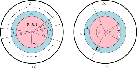
Figure 4: Sketch of the proof idea for Proposition 4.7. (a) Illustration of the set of points $\mathcal{A}$ (blue) of width $\xi$ slightly outside of the core (pink). The intersection with a sector of angle $\psi$ and the band $\mathcal{A}$ forms a box $\mathcal{A}_{i}$ that contains a vertex w.e.h.p. The number of non-intersecting boxes is $k=2\pi/\psi\in\omega(\log(n))$. (b) A box $\mathcal{A}_{i}$ that contains vertex $u$. The hatched area $\mathcal{F}_{u}$ with angle at most $\phi$ is the corresponding forbidden area of $u$. Any point in $\operatorname{\mathcal{F}_{u}}$ has distance at least $R$ to $u$. An adequate choice for the width $\xi$ yields that this area is empty with constant probability.

For the proof we consider the Poissonized version of the HRG model (see e.g. [24, 25]). The upshot of this model is that it allows us to analyse disjoint areas in the hyperbolic disk independently. Since the final result holds w.e.h.p. this directly carries over to the uniform model w.e.h.p. ([21, Lemma 3.9]). We start by defining an area $\mathcal{A}$ close to the core. Let $\xi=\log\left(1+\frac{\log^{3}(n)}{n^{1-\alpha}}\right)\in o(1)$ and consider a band of points $\mathcal{A}:=\mathcal{B}_{0}(R/2+\xi)\setminus\mathcal{B}_{0}(R/2)$. We see via $R=2\log(n)+C$ that

$$\begin{split}\mu(\mathcal{A})&=\int_{R/2}^{R/2+\xi}\frac{\sinh(\alpha x)}{\cosh(\alpha R)-1}=\frac{\cosh(\alpha(R/2+\xi))-\cosh(\alpha R/2)}{\cosh(\alpha R)-1}\\ &=(1+\Theta(e^{-\alpha R}))(e^{-\alpha(R/2-\xi)}-e^{-\alpha R/2})\\ &=(1+\Theta(e^{-\alpha R}))(n^{-\alpha}e^{-\alpha C/2}{\left(1+\log^{3}(n)n^{\alpha-1}\right)}-n^{-\alpha}e^{-\alpha C/2})\\ &=(1+\Theta(e^{-\alpha R}))\big{(}e^{-\alpha C/2}\log^{3}(n)n^{-1}\big{)}\in\Theta\left(\log\left(n^{3}/n\right)\right).\end{split}$$ (3)

Let $A=V\cap\mathcal{A}$. Then $\mathbb{E}[|A|]\in\Theta\left(\log^{3}(n)\right)$. We further partition the band $\mathcal{A}$ into $k=\lceil\log^{3/2}(n)\rceil$ sectors $\mathcal{A}_{1},\ldots,\mathcal{A}_{k}$, each of equal size (see Figure 4 a), and $A_{i}=V\cap\mathcal{A}_{i}$. Since $\mathbb{E}[|A|]\in\Theta\left(\log^{3}(n)\right)$ and $k=\log^{3/2}(n)$, we have for any $i\in[k]$ that $\mathbb{E}[|A_{i}|]=\frac{\mathbb{E}[|A|]}{k}\in\omega(\log(n))$. Since we are in the Poissonized model we get $\mathbb{P}\left(|A_{i}|=0\right)=e^{-\mathbb{E}\left[|A_{i}|\right]}\in n^{-\omega(1)}.$ Subsequently, a union bound yields that there is no sector $\mathcal{A}_{i}$ that is empty w.e.h.p.

In the second step, we show that for any vertex $u\in A$, the probability that there exists a vertex in its forbidden area $\operatorname{\mathcal{F}_{u}}$ is strictly less than $1$. Since $r(u)\leq R/2+\xi$, we have that $u\in A$ has an edge to any vertex in the area $\mathcal{B}_{0}(R/2-\xi)$. Hence, we have $\operatorname{\mathcal{F}_{u}}\subset\mathcal{B}_{0}(R/2)\setminus\mathcal{B}_{0}(R/2-\xi)$. Now, for $R/2\geq x\geq R/2-\xi$ we seek to find the angle size $\phi=2(\pi-\theta_{R}(r(u),x))$ in order to upper bound $\mu(\operatorname{\mathcal{F}_{u}})$. Since $\theta_{R}(r,x)$ is monotonically decreasing in $x$ we have $\phi\leq 2(\pi-\theta_{R}(R/2+\xi,R/2))$ and we obtain

$$\mu(\operatorname{\mathcal{F}_{u}})=\int_{R/2-\xi}^{R/2}\int_{0}^{\phi}\rho(x)\,\mathrm{d}\phi\,\mathrm{d}x \leq 2(\pi-\theta_{R}(R/2+\xi,R/2))\int_{R/2}^{R/2+\xi}\rho(x)\,\mathrm{d}x$$

$$\leq 2(\pi-\theta_{R}(R/2+\xi,R/2))\mu(\mathcal{A}),$$

where we used $\int_{R/2-\xi}^{R/2}\rho(x)\,\mathrm{d}x\leq\int_{R/2}^{R/2+\xi}\rho(x)\,\mathrm{d}x=\mu(\mathcal{A})$. By our choice of $\xi=\log(1+\log^{3}(n)n^{\alpha-1})\in o(1)$, we can apply Lemma B.5 and obtain $\theta_{R}(R/2+\xi,R/2)\geq\pi-2\sqrt{\frac{\log^{3}(n)}{n^{1-\alpha}}}$. In Equation 3 we established that $\mu(\mathcal{A})\in\Theta\left(\log^{3}\left(n\right)/n\right)$. Combining the two leads to $\mu(\operatorname{\mathcal{F}_{u}})\in\mathcal{O}\Big{(}\sqrt{\log^{9}(n)n^{\alpha-3}}\Big{)}$.

Notice that for $\alpha\in(1/2,1)$, the measure of the forbidden area of a vertex $u\in A$ is $\mu(\operatorname{\mathcal{F}_{u}})\in o(1/n)$. Hence, writing $F=V\cap\operatorname{\mathcal{F}_{u}}$, we get $\mathbb{E}[|F|]\in o(1)$, i.e., the expected number of vertices in $\operatorname{\mathcal{F}_{u}}$ is vanishing. Applying Markov’s inequality then gives us $\mathbb{P}\left(|F|\geq 1\right)\in o(1)$. Thus $p\coloneqq\mathbb{P}(|F|<1)\in\Omega(1)$, so the forbidden area is empty with constant probability.

We now establish our third and final desired property. Namely, we construct a subset $U\subset A$, consisting of vertices whose forbidden areas are disjoint and for which $\mathbb{E}\left[|U|\right]\in\omega(\log(n))$.

Recall that we partitioned $\mathcal{A}$ into $k=\log^{3/2}(n)\in\omega(\log(n))$ sectors. Let $X_{i}$ be the indicator that there exists a vertex $u\in\mathcal{A}_{i}$ whose forbidden area $\operatorname{\mathcal{F}_{u}}$ is empty. Then $X=\sum_{i=1}^{\lfloor k/2\rfloor}X_{2i}$ is a loose lower bound on the number of sectors with this property. By linearity of expectation, $p$ constant and $k=\log^{3/2}(n)$ we then obtain

$$\mathbb{E}[X]\geq\mathbb{E}\Big{[}\sum_{i=1}^{\lfloor k/2\rfloor}X_{2i}\Big{]}\geq p\cdot\Theta(1)\log^{3/2}(n)\in\omega(\log(n)).$$

We proceed by showing independence among the random variables $X_{i}$ and $X_{j}$ for $|j-i|>1$. To this end, observe that the angle $\psi$ (see Figure 4 b) spanned by any sector $\mathcal{A}_{i}$ is $\psi=2\pi/k\geq\left\lfloor 2\pi\log^{-3/2}(n)\right\rfloor$. In contrast, we recall $\phi\leq 2(\pi-\theta_{R}(R/2+\xi,R/2))\leq 4\sqrt{\log^{3}(n)n^{\alpha-1}}$. Since $\sqrt{\log^{3}(n)n^{\alpha-1}}\in o(\log^{-3/2}(n))$ we conclude $\phi\in o(\psi)$. This implies that the forbidden areas $\mathcal{F}_{u}$ and $\mathcal{F}_{v}$ of any $u\in\mathcal{A}_{i}$, $v\in\mathcal{A}_{j}$ are disjoint. Thus $X_{i}$ and $X_{j}$ are independent.

To wrap things up, recall that in the first step we established that each sector $\mathcal{A}_{i}$ contains a vertex w.e.h.p. Moreover, since the $X_{i}$ are independent, we have by a Chernoff bound (Theorem A.1) that $X\in\omega(\log(n))$ w.e.h.p. Though these two events are not independent, we can apply the union bound to their complements to obtain that w.e.h.p. $\omega(\log(n))$ vertices outside of $\mathcal{B}_{0}(R/2)$ are adjacent to all vertices in $\mathcal{B}_{0}(R/2)$, which finishes the proof.

4.3 Upper Bound on the Clique Number

Recall that two vertices $u,v$ are adjacent if and only if $\operatorname{d_{h}}(u,v)\leq R$ and that we call the clique formed in $\mathcal{B}_{0}(R/2)$ the core whose size is $\sigma(G)=(1-o(1))e^{-\alpha C/2}n^{1-\alpha}$ w.e.h.p. The core size is a lower bound for the clique number $\omega(G)$. We have established that the largest clique is smaller than the degeneracy w.e.h.p. (Theorem 4.3), and in this section we further investigate an upper bound for $\omega(G)$. We note that the upper bound we derive in this section implies Theorem 4.3 for $\alpha$ large enough (see Figure 1). However, for smaller $\alpha$, the upper bound for $\omega(G)$ is larger than the lower bound (Theorem 3.5) for $\kappa(G)$ in the HRG model, and thus does not directly imply Theorem 4.3 for these values for $\alpha$.

Before going into details, we lay out our proof strategy. We aim to bound the region where a clique can be located. Since vertices are adjacent if and only if their (hyperbolic) distance is at most $R$, this can be done by characterising a shape that covers any hyperbolic region of diameter $R$. A classic result by Jung [19] answers the question of how large the radius of a ball in Euclidean space needs to be at most, so that its interior can contain an entire set of points of fixed diameter. The hyperbolic version of this result was discovered by Dekster [13, 14] nearly a century later. He extended Jung’s result to (among other geometries) hyperbolic space and we apply it as follows: we identify $\mathcal{O}(n^{3})$ many balls where one of these balls contains the clique of largest of size $\omega(G)$. This clique (and all the other identified cliques) needs to be located in a ball $B_{x}(r)$ with radius $r$ large enough. We use the hyperbolic variant of Jung’s theorem to upper bound $r$ which, in turn, allows us to upper bound the area of this ball. This yields an upper bound for the amount of vertices one such ball $B_{x}(r)$ could contain w.e.h.p., leading to an upper bound for $\omega(G)$. Since we need only consider at most $\mathcal{O}(n^{3})$ balls, a union bound is sufficient to derive the same bound for the worst case. We work with the following version of Jung’s theorem for hyperbolic geometry.

Corollary 4.9.

Let $\mathcal{K}\subset\mathbb{H}^{2}$ be compact and suppose that for any $y,z\in\mathcal{K}$, $\operatorname{d_{h}}(y,z)\leq R$. Then there exists $x\in\mathbb{H}^{2}$ such that $\mathcal{K}\subseteq\mathcal{B}_{x}(r)$ for $r$ satisfying $r\leq R/2+\log(2/\sqrt{3})$.

Our next observation follows from the definition of $\mu$, and formalises the intuition that $\mu$ puts more mass at the centre of the disk. Let $0<r\leq R$ and $u,v\in\mathcal{D}_{R}$ with $r(u)\geq r(v)$. Then $\mu(\mathcal{B}_{u}(r))\leq\mu(\mathcal{B}_{v}(r))$.

Recall that $\sigma(G)$ denotes the core size $|V\cap\mathcal{B}_{0}(R/2)|$ which is a lower bound for the clique number $\omega(G)$ (see Section 3), and that $\sigma(G)=(1-o(1))e^{-\alpha C/2}n^{1-\alpha}$ w.e.h.p. We state our upper bound relative to this lower bound.

Theorem 4.10 (Clique upper bound).

Let $G\sim\mathcal{G}(n,\alpha,C)$ be a threshold HRG with $\alpha\in(1/2,1)$. Then w.e.h.p.

$$\omega(G)\leq\left((4/3)^{\alpha/2}+o(1)\right)\sigma(G).$$

Proof 4.11.

Consider any triplet of vertices $u,v,w\in V$ with pairwise distance at most $R$, so that they are pairwise adjacent. Since $u,v,w$ are a.s. in general position, there is a unique ball $\mathcal{B}_{x}(r)$ such that $u,v,w$ lie on the boundary $\partial\mathcal{B}_{x}(r)$. By Corollary 4.9, $r\leq R/2+\log(\sqrt{4/3})$ since $\max{(\operatorname{d_{h}}(u,v),\operatorname{d_{h}}(v,w),\operatorname{d_{h}}(u,w))}\leq R$. Over all possible triplets $u,v,w\in V$ this gives us a set $B$ of at most $n\choose 3$ closed balls. Any clique must be contained in one of these balls, and therefore so is the largest clique. Thus upper bounding the number of vertices for each individual ball $\mathcal{B}\in B$ yields an upper bound on the size of the largest clique.

We now upper bound the expected number of vertices in one ball $B$. To this end we fix a ball $\mathcal{B}=\mathcal{B}_{x}(r)\in B$ and let $Y_{\mathcal{B}}$ be the random variable counting the number of vertices in $\mathcal{B}$. The balls in $B$ are identically (though clearly not independently) distributed. Since vertices are thrown independently according to $\mu$, we have that $Y_{\mathcal{B}}-3\sim\mathrm{Bin}(n-3,\mu(\mathcal{B}))$, and so

$$\mathbb{E}\left[Y_{\mathcal{B}}\right]=3+(n-3)\mu(\mathcal{B}) \leq 3+(n-3)\mu(\mathcal{B}_{0}(r))$$ (Section 4.3)

$$\leq 3+(n-3)\mu(\mathcal{B}_{0}(R/2+\log(2/\sqrt{3})))$$ (Corollary 4.9)

$$\leq\big{(}\big{(}2/\sqrt{3}\big{)}^{\alpha}+o(1)\big{)}e^{-\alpha C/2}n^{1-\alpha}.$$ (Equation 2)

Thus $((4/3)^{\alpha/2}+o(1))\sigma(G)\geq(1+1/\log(n))\mathbb{E}\left[Y_{\mathcal{B}}\right]$ w.e.h.p. This is relevant to the bound in the theorem statement because it implies that

$$\mathbb{P}\Big{(}\omega(G)>((4/3)^{\alpha/2}+o(1))\sigma(G)\Big{)} \leq\mathbb{P}\Big{(}\max_{\mathcal{B}\in B}Y_{\mathcal{B}}>((4/3)^{\alpha/2}+o(1))\sigma(G)\Big{)}$$

$$\leq\mathbb{P}\Big{(}\max_{\mathcal{B}\in B}Y_{\mathcal{B}}>(1+1/\log(n))\mathbb{E}[Y_{\mathcal{B}}]\Big{)}+n^{-c}$$

for arbitrary $c$. Thus to finish the proof we need to show concentration, which via a union bound over all triplets $u,v,w$ will yield the result. To show concentration we apply a Chernoff bound. Using $\varepsilon=(1/\log(n))$ we obtain

$$\mathbb{P}\left(Y_{\mathcal{B}}>(1+1/\log(n))\mathbb{E}[Y_{\mathcal{B}}]\right) \leq e^{-(1/\log(n))^{2}/3\cdot\mathbb{E}[Y_{\mathcal{B}}]}\leq e^{-\Theta(1)(n^{1-\alpha})/\log^{2}(n)}\leq n^{-c}$$

for any choice of $c$, since for $\alpha<1$, $\Theta(1)(n^{1-\alpha})\in n^{\Theta(1)}$ and $\liminf_{n\to\infty}\frac{n^{\Theta(1)}}{\log^{2}(n)}\in\omega(\log(n)).$ Finally, to show that this holds w.e.h.p. for all balls in $B$, we use that $|B|\leq{n\choose 3}<n^{3}$, so that

$$\mathbb{P}\Big{(}\max_{\mathcal{B}\in B}Y_{\mathcal{B}}\geq(1+1/\log(n))\mathbb{E}[Y_{\mathcal{B}}]\Big{)} \leq\sum_{\mathcal{B}\in B}\mathbb{P}\left(Y_{\mathcal{B}}\geq(1+1/\log(n))\mathbb{E}[Y_{\mathcal{B}}]\right)$$

$$\leq n^{3}\mathbb{P}\left(Y_{\mathcal{B}}\geq(1+1/\log(n))\mathbb{E}[Y_{\mathcal{B}}]\right)\leq n^{-c+3}.\qed$$

A further refinement of the “clique covering” argument of Theorem 4.10 should be possible. Any clique has by definition a diameter of at most $R$, and so the shape in $\mathbb{H}^{2}$ of diameter $R$ with maximal area would provide an improved upper bound via a similar covering argument. It is not clear what a tight bound would be, and $\omega(G)\leq(1+o(1))\sigma(G)$ may be possible.

5 Geometric Inhomogeneous Random Graphs

Geometric Inhomogeneous Random Graphs or GIRGs were introduced in [10] as an alternative model to HRGs that capture many of the same properties, in particular the power-law degree distribution. In their most general form, GIRGs strictly generalise HRGs, but they are more often studied in a slightly restricted form; comparisons are made in [5, 26]. In this restricted form, called the standard GIRG model by [15], any HRG $G$ can be coupled with two GIRGs $H_{1}$ and $H_{2}$ such that $H_{1}\subseteq G\subseteq H_{2}$, where $\subseteq$ denotes graph inclusion.

Because of this relationship, GIRGs are used as proxies for HRGs in some theoretical and experimental works. This is partly done because GIRGs are (by design) far more tractable than HRGs. It is therefore valuable to understand differences between the two models. In [5] experimental evidence was given to suggest that the “sandwiching” of an HRG by two standard GIRGs is not tight. In Corollary 5.5 we provide theoretical result demonstrating a difference between the two models.

Definition 5.1 (Standard GIRG model).

Let $\beta\in(2,3)$, $\lambda\in\Theta(1)$, and $n\in\mathbb{N}$. A geometric inhomogeneous random graph $G\sim\mathcal{G}(n,\beta,\lambda)$ is a random graph with vertex set $V=\{v_{1},\cdots,v_{n}\}$ satisfying the following properties.

1. Every $u\in V$ is equipped with a random tuple $(w_{u},x_{u})$, where $w_{u}\in[1,\infty)$ has density $f(y)=(\beta-1)y^{-\beta}$ and $x_{u}$ is drawn uniformly at random from $[0,1]$;

2. Any pair of vertices $u,v\in V$ are connected if and only if $\min\{|x_{u}-x_{v}|,1-|x_{u}-x_{v}|\}\leq t(u,v)$, where $t(u,v)=\frac{1}{2}\left(\frac{\lambda w_{u}w_{v}}{n}\right)$.

One way of thinking of a GIRG is that vertices are being thrown uniformly at random onto the 1-dimensional torus $\mathbb{T}^{1}$, and connected according to whether their distance is below threshold $t(u,v)$. Analogously to HRGs, for a vertex $u$ of a GIRG we define the inner-degree of $u$ to be $|\operatorname{\Gamma}(u)|=|\{v\in V|\text{$u$ and $v$ are connected and }w_{v}\geq w_{u}\}|.$ The proofs of Sections 3 and 3.2 can be adapted to the GIRG model to characterize the degeneracy via the largest inner-degree.

Corollary 5.2.

Let $G\sim\mathcal{G}(n,2\alpha+1,\lambda)$ be a standard GIRG. Consider the vertex $u^{*}$ with the largest inner-degree in $G$. Then w.e.h.p. $\kappa(G)=(1-o(1))|\operatorname{\Gamma}(u^{*})|.$

Corollary 5.2 allows us to state a tight bound for the degeneracy in comparison to the core of the GIRG, which is defined to contain all vertices of weight $\hat{w}\geq\sqrt{n/\lambda}$, and has size $\sigma(G)=(1\pm o(1))\lambda^{-\alpha}n^{1-\alpha}$ w.e.h.p. This is analagous to the core of an HRG, which is the clique formed by vertices of radius at most $R/2$, regardless of their angular coordinates.

Theorem 5.3.

Let $G\sim\mathcal{G}(n,2\alpha+1,\lambda)$ be a threshold GIRG. The degeneracy is w.e.h.p.

$$\kappa(G)=(2\pm o(1))(2(1-\alpha))^{({1-\alpha})/{(2\alpha-1)}}\sigma(G).$$

Proof 5.4 (Proof sketch).

We prove the statement in three steps. First, we compute the probability for a vertex $v$ to lie in the inner-neighbourhood of a vertex $u$ depending on the weight $w_{u}$. We then use this to find the weight $w^{*}$ maximising expected inner-neighbourhood. Combining the two, we use $w^{*}$ to obtain upper- and lower bounds on the largest inner-degree of a vertex w.e.h.p. The statement then follows from Corollary 5.2.

Comparing the lower bound of the degeneracy for GIRGs given in Theorem 5.3 to the upper bound of a HRG we obtained in Theorem 3.5 we draw the conclusion that the degeneracy-to-core ratio between the two models is fundamentally different.

Corollary 5.5.

Fix an $\alpha\in(1/2,1)$, and let $G\sim\mathcal{G}(n,2\alpha+1,\lambda)$ be a standard GIRG and $H\sim\mathcal{G}(n,\alpha,C)$ be a threshold HRG. Then w.e.h.p.

$$\left|\frac{\kappa(G)}{\sigma(G)}-\frac{\kappa(H)}{\sigma(H)}\right|\in\Theta(1).$$

6 Conclusion

We have shown that the clique number, degeneracy, and chromatic number of HRGs are asymptotically (with small differences in the leading $O$-notation constants) as large as the core, though the clique number and degeneracy differ significantly. Our upper bound on the degeneracy provides a constant factor approximation algorithm for the graph colouring problem. The approximation ratio ranges from $2/\sqrt{3}$ to $4/3$ and depends on the model parameter $\alpha$. This raises several open questions and future research directions.

• Is the chromatic number bounded away from the degeneracy, the clique number, or from both?

• Can HRGs be coloured optimally in polynomial time or is it NP-complete?

• What are the asymptotics of $\omega(G)/\sigma(G)$? Is the clique number a constant factor larger than the core and has similar behaviour as the degeneracy?

• Can the gap between upper and lower bound for the clique number be closed?

There are several further directions of research such as determining further differences between HRGs and GIRGs or designing colouring and other algorithms for HRGs in various models of computation.

Appendix A Concentration bounds

We frequently use the following Chernoff bounds [30, Theorem 4.4].

Theorem A.1 (Chernoff bound).

For $i\in[k]$, let $X_{i}\in\{0,1\}$ be independent random variables and $X=\sum_{i}X_{i}$. Then for $\varepsilon\in(0,1)$,

$$\mathbb{P}\left(X\geq(1+\varepsilon)\mathbb{E}[X]\right)\leq e^{-\varepsilon^{2}/3\cdot\mathbb{E}[X]}\text{ and }\mathbb{P}\left(X\leq(1-\varepsilon)\mathbb{E}[X]\right)\leq e^{-\varepsilon^{2}/2\cdot\mathbb{E}[X]}.$$

Appendix B Bounds on $\theta_{R}(\cdot,\cdot)$

Before we give bounds on the measure of areas in Appendix C, we provide some refined bounds on $\theta_{R}(r,q)$ for several pair of radii with $r+q\geq R+\Delta$ for specific $\Delta\in\Theta(1)$. This will prove useful since the considered inner-neighbourhoods belong to vertices that are close to the core ball $\mathcal{B}_{0}(R/2)$. We use the following inequality for the $\arccos$.

Lemma B.1.

Let $0<\varepsilon\leq x\leq z\leq 2$. Then

$$\arccos(1-\varepsilon)\sqrt{x/\varepsilon}\leq\arccos(1-x)\leq\arccos(1-z)\sqrt{x/z}.$$

Proof B.2.

The statement follows by observing that $\arccos(1-x)x^{-1/2}$ is increasing in $x$ for domain $(0,2]$.

Recall that $\theta_{R}(r,q)$ is the angle between points with radii $p$ and $q$ such that the distance between them is $R$. We apply Lemma B.1 to $\theta_{R}(r,q)$ to obtain the following.

Lemma B.3.

For $u,v\in\mathcal{D}_{R}$ and $\Delta\in\Theta(1)$, let $r(u)=r\geq q=r(v)$ and $r+q=R+\Delta$. Then there exists a constant $\delta>0$, such that

$$(2+\delta)\sqrt{e^{R-r-q}}<\theta_{R}(r,q)\leq\begin{cases}\pi\sqrt{e^{R-r-q}}&\text{ for }\Delta\geq 0,\\ \frac{4\pi}{3\sqrt{3}}\sqrt{e^{R-r-q}}&\text{ for }\Delta\geq\log(4/3),\\ \frac{\pi}{\sqrt{2}}\sqrt{e^{R-r-q}}&\text{ for }\Delta\geq\log(2),\\ \frac{2\pi}{3}\sqrt{e^{R-r-q}}&\text{ for }\Delta\geq 2\log(2).\end{cases}$$

Proof B.4.

We adapt the proof of [6, Lemma 4]. Let us start with the upper bounds. We take advantage of the fact that $\arccos$ is a decreasing function. This means that we can upper bound $\theta_{R}(r,q)$:

$$\theta_{R}(r,q)=\arccos\left(\frac{\cosh(r)\cosh(q)-\cosh(R)}{\sinh(r)\sinh(q)}\right)\leq\arccos\left(1-2e^{R-r-q}\right).$$

Since $2e^{R-r-q}\in\left(0,2e^{-\Delta}\right]$ we can apply Lemma B.1. Evaluating the $\arccos$ for $r+q=R+\Delta$ for the domains of our interest we obtain

$$\arccos\left(1-2e^{R-r-q}\right)\leq\begin{cases}\pi&\text{ for }\Delta\geq 0,\\ \frac{2\pi}{3}&\text{ for }\Delta\geq\log(4/3),\\ \frac{\pi}{2}&\text{ for }\Delta\geq\log(2),\\ \frac{\pi}{3}&\text{ for }\Delta\geq 2\log(2),\end{cases}$$

and the respective upper bound for $\theta_{R}(r,q)$ and each domain follows.

We now show a lower bound for $\theta_{R}(r,q)$. Since $\arccos$ is monotonic decreasing we upper bound its inner term to lower bound $\theta_{R}(r,q)$. By the identity $\cosh(r)\cosh(q)=\sinh(r)\sinh(q)-\cosh(r-q)$, we get

$$\theta_{R}(r,q) =\arccos\left(\frac{\cosh(r)\cosh(q)-\cosh(R)}{\sinh(r)\sinh(q)}\right)$$

$$=\arccos\left(1-\frac{\cosh(R)-\cosh(r-q)}{\sinh(r)\sinh(q)}\right)$$

$$\geq\arccos\left(1-2e^{R-r-q}+e^{-R-r-q}-\left(e^{-2q}+e^{-2r}\right)\right).$$

Note that, by our hypothesis that $q\leq r\leq R/2+\mathcal{O}(1)$, there exists an $\varepsilon>0$, such that $2e^{R-x-y}+e^{-R-x-y}-\left(e^{-2x}+e^{-2r}\right)\in\left[\varepsilon,2\right)$. Thus, we can and we will apply Lemma B.1. We note that, for all $\varepsilon>0$ there exists a constant $\delta^{\prime}>0$ such that $\arccos(1-\varepsilon)\sqrt{\frac{2}{\varepsilon}}=2+\delta^{\prime}$. Hence there exists another constant $\delta$ such that $0<\delta<\delta^{\prime}$, for which we get

$$\arccos\left(1-2e^{R-r-q}+e^{-R-r-q}-\left(e^{-2q}+e^{-2r}\right)\right)$$

$$\geq(2+\delta^{\prime})\sqrt{e^{R-r-q}+\frac{e^{-R-r-q}-\left(e^{-2q}+e^{-2r}\right)}{2}}\geq(2+\delta)\sqrt{e^{R-r-q}},$$

since $\left(e^{-2q}+e^{-2r}\right)\in\mathcal{O}(1/n)$ by $r\geq x\geq R/2=\log(n)$ + C/2.

We also consider vertices that have a sub-constant distance to the core. The statement here tells us that when $r$ approaches $R/2$ from above, the angle $\theta_{R}(r,R/2)$ approaches $\pi$ from below.

Lemma B.5.

Let $k\in\mathbb{N}\setminus\{0\}$ and $\xi_{k}=\log(1+\frac{\log^{k}(n)}{n^{1-\alpha}})\in o(1)$. Consider two points with radial coordinates $r=R/2+\xi_{k}$ and $x=R/2$. Then $\theta_{R}(r,x)\geq\pi-2\sqrt{\log^{k}(n)n^{\alpha-1}}$.

Proof B.6.

Since $\arccos$ is a monotonically decreasing function and we aim to lower bound $\theta_{R}(r,x)$, we apply the identity $\cosh(r)\cosh(x)=\sinh(r)\sinh(x)+\cosh(r-x)$ and get

$$\theta_{R}(r,x) \geq\arccos\left(1-2\left(e^{R-r-x}+e^{-R-r-x}-\left(e^{-2r}+e^{-2x}\right)\right)\right).$$

Next, we apply $r+x=R+\xi_{k}$ and $R=2\log(n)+C$ which leads to

$$\theta_{R}(r,x) \geq\arccos\left(1-2\left(e^{-\xi_{k}}+e^{-(4\log(n)+2C+\xi_{k})}-\left(e^{-2r}+e^{-2x}\right)\right)\right)$$

$$\geq\arccos\left(1-2\left(e^{-\xi_{k}}+e^{-(4\log(n)+2C+\xi_{k})}-2e^{-(2\log(n)+C)}\right)\right),$$

where we applied $r>x=R/2$ in the second line. Using again the fact that $\arccos$ is a monotonically decreasing function we have

$$\theta_{R}(r,x) \geq\arccos\left(1-2\left(e^{-\xi_{k}}-2e^{-(2\log(n)+C)}\right)\right).$$

Note that for $\xi_{k}\in o(1)$ and $n$ approaching infinity the term $2\left(e^{-\xi_{k}}-2e^{-(2\log(n)+C)}\right)$ approaches $2$ from below. Hence, a Taylor expansion around $n=\infty$ now yields

$$\theta_{R}(r,x) \geq\pi-2\sqrt{\log^{k}(n)n^{\alpha-1}},$$

as required.

Appendix C Lemma 3.4

Lemma B.3 allows us to bound the probability of a vertex $v$ belonging to the inner-neighbourhood area of a vertex $u$. We remark that these bounds are sharper than the ones obtained in [7, Lemma 3] for points with radius $R/2+\Theta(1)$. In contrast, for points with radius $R/2+\omega(1)$ the bound in [7, Lemma 3] is superior. Moreover, notice that for vertices with radius $r\leq R/2$, the inner-neighbourhood is simply $V\cap\mathcal{B}_{0}(r)$.

Lemma C.1.

Let $\Delta\in[0,R/2)$ and consider a point $u$ with radial coordinate $r=R/2+\Delta$. Then, for the inner-ball $\mathcal{I}(r)$,

$$\mu(\mathcal{I}(r))\leq\left(1+\Theta\left(e^{-\alpha R}\right)\right)\frac{\alpha e^{-\alpha r}}{\alpha-1/2}\left(\gamma e^{\frac{1}{2}(2\alpha-1)(2r-R)}-\eta\right),$$

where

$$\gamma,\eta=\begin{cases}1,\frac{1}{2\alpha}&\text{ for }\Delta\geq 0,\\ \frac{4}{3\sqrt{3}},\frac{1}{2\alpha}-\left(1-\frac{4}{3\sqrt{3}}\right)\left(\frac{4}{3}\right)^{(\alpha-1/2)}&\text{ for }\Delta\geq\log(\sqrt{4/3}),\\ \frac{1}{\sqrt{2}},\frac{1}{2\alpha}-\left(1-\frac{4}{3\sqrt{3}}\right)\left(\frac{4}{3}\right)^{(\alpha-1/2)}-\left(\frac{4}{3\sqrt{3}}-\frac{1}{\sqrt{2}}\right)2^{(\alpha-1/2)}&\text{ for }\Delta\geq\log(\sqrt{2}),\\ \frac{2}{3},\frac{1}{2\alpha}-\left(1-\frac{4}{3\sqrt{3}}\right)\left(\frac{4}{3}\right)^{(\alpha-1/2)}-\left(\frac{4}{3\sqrt{3}}-\frac{1}{\sqrt{2}}\right)2^{(\alpha-1/2)}-\left(\frac{1}{\sqrt{2}}-\frac{2}{3}\right)2^{(2\alpha-1)}&\text{ for }\Delta\geq\log(2).\\ \end{cases}$$

Proof C.2.

The proof is an adaptation of [18, Lemma 3.2]. We calculate the measure of the inner-ball by integrating over the desired area. Since a vertex $u$ with radius $r$ has $\operatorname{d_{h}}(u,v)\leq R$ if $r(v)\leq R-r$ we have for the area of an inner-ball

$$\mu(\mathcal{I}(r)) =\mu(\mathcal{B}_{u}(R)\cap\mathcal{B}_{0}(r))=\mu(\mathcal{B}_{0}(R-r))+2\int_{R-r}^{r}\int_{0}^{\theta_{R}(x,r)}\rho(x)\,\mathrm{d}\theta dx.$$

By Lemma B.3 we have $\theta_{R}(r,q)\leq\pi\sqrt{e^{(R-r-x)}}$ for $x+r\geq R$. Thus, for every $x\in[R-r,r]$, there exists a $\tau\leq\pi$ such that

$$\mu(\mathcal{B}_{0}(R-r))+2\int_{R-r}^{r}\tau e^{\frac{R-r-x}{2}}\frac{\alpha\sinh(\alpha x)}{2\pi(\cosh(\alpha R)-1)}dx$$

$$=\mu(\mathcal{B}_{0}(R-r))+\frac{\alpha e^{(R-r)/2}}{\pi(\cosh(\alpha R)-1)}\int_{R-r}^{r}\tau e^{-x/2}\sinh(\alpha x)dx.$$

Notice that we can split the integral of the domain $[R-r,r]$ into further sub domains such that for domain $[s,t]$ we get $s+r\in R+\Theta(1)$. This allows to apply different bounds for $\theta_{R}(s,r)$ as shown in Lemma B.3, giving a more refined upper bounds on $\tau$. Thus, we apply Lemma B.3 to obtain

$$\mu(\mathcal{I}(r)) \leq\mu(\mathcal{B}_{0}(R-r))$$ (4)

$$\quad+\operatorname{\mathbf{1}}_{\{r\geq R/2\}}\frac{\alpha e^{(R-r)/2}}{(\cosh(\alpha R)-1)}\int_{R-r}^{\min(r,R-r+\log(4/3))}e^{-x/2}\sinh(\alpha x)\,\mathrm{d}x$$ (5)

$$\quad+\operatorname{\mathbf{1}}_{\{r\geq R/2+\log(\sqrt{4/3})\}}\frac{{4}\alpha e^{(R-r)/2}}{{3\sqrt{3}}(\cosh(\alpha R)-1)}\int_{R-r+\log(4/3)}^{\min(r,{R-r+\log(2)})}e^{-x/2}\sinh(\alpha x)\,\mathrm{d}x$$ (6)

$$\quad+\operatorname{\mathbf{1}}_{\{r\geq R/2+\log(\sqrt{2})\}}\frac{\alpha e^{(R-r)/2}}{\sqrt{2}(\cosh(\alpha R)-1)}\int_{R-r+\log(2)}^{{\min(r,R-r+2\log(2))}}e^{-x/2}\sinh(\alpha x)\,\mathrm{d}x$$ (7)

$$\quad+\operatorname{\mathbf{1}}_{\{r\geq R/2+2\log(\sqrt{2})\}}\frac{2\alpha e^{(R-r)/2}}{3(\cosh(\alpha R)-1)}\int_{R-r+2\log(2)}^{r}e^{-x/2}\sinh(\alpha x)\,\mathrm{d}x.$$ (8)

Before we consider each desired case for $\Delta$ separately, we observe that each integral is of the form $\int_{s}^{t}e^{-x/2}\sinh(\alpha x)\,\mathrm{d}x$. Doing the calculations yield

$$\int_{s}^{t}e^{-x/2}\sinh(\alpha x) =\left[\frac{2}{4\alpha^{2}-1}e^{-x/2}(2\alpha\cosh(\alpha x)+\sinh(\alpha x))\right]_{s}^{t}$$

$$=\frac{2}{4\alpha^{2}-1}\left(e^{-t/2}(2\alpha\cosh(\alpha t)+\sinh(\alpha t))\right)$$

$$-\frac{2}{4\alpha^{2}-1}\left(e^{-s/2}(2\alpha\cosh(\alpha s)+\sinh(\alpha s)\right).$$

We note that each for $y,z\in\mathbb{Q}$ and $k,m\in\mathbb{N}$, we can write $s$ as $R-r+k\log(y)$ and $t$ either as $k^{\prime}\log(z)$ or $r$. First we plug in $s=R-r+k\log(y)$ and $t=R-r+k^{\prime}\log(z)$ and get

$$(4\alpha^{2}-1) e^{(R-r)/2}\int_{R-r+k\log(y)}^{R-r+k^{\prime}\log(z)}e^{-x/2}\sinh(\alpha x)$$

$$=2(z^{-k^{\prime}/2}(2\alpha\cosh(\alpha(R-r+k^{\prime}\log(z)))+\sinh(\alpha(R-r+k^{\prime}\log(z))))$$

$$\quad-2(y^{-k/2}(2\alpha\cosh(\alpha(R-r+k\log(y)))+\sinh(\alpha(R-r+k\log(y))))$$

$$=2(z^{-k^{\prime}/2}(z^{k^{\prime}\alpha}(\alpha+1/2)e^{\alpha(R-r)}+z^{-k^{\prime}\alpha}(\alpha-1/2)e^{-\alpha(R-r)}))$$

$$\quad-2(y^{-k/2}(y^{k\alpha}(\alpha+1/2)e^{\alpha(R-r)}+y^{-k\alpha}(\alpha-1/2)e^{-\alpha(R-r)})$$

$$=(2\alpha+1)\left(z^{k^{\prime}(\alpha-1/2)}e^{\alpha(R-r)}-y^{k(\alpha-1/2)}e^{\alpha(R-r)}\right)$$

$$\quad-(2\alpha-1)\left(y^{-k(1/2+\alpha)}e^{-\alpha(R-r)}-z^{-k^{\prime}(\alpha+1/2)}e^{-\alpha(R-r)}\right)$$

$$\leq(2\alpha+1)\left(z^{k^{\prime}(\alpha-1/2)}-y^{k(\alpha-1/2)}\right)e^{\alpha(R-r)}\qquad \alpha>1/2$$ (since )

Multiplying both sides by $\tau\alpha/\pi(4\alpha^{2}-1)(\cosh(\alpha R)-1)$, and noting that $(\cosh(\alpha R)-1)^{-1}=2\exp({-\alpha R})\left(1+\Theta\left(e^{-\alpha R}\right)\right)$, yields

$$\begin{split}\frac{\tau\alpha e^{(R-r)/2}}{\pi(\cosh(\alpha R)-1)}&\int_{R-r+k\log(y)}^{R-r+k^{\prime}\log(z)}e^{-x/2}\sinh(\alpha x)\\ &\leq\left(1+\Theta\left(e^{-\alpha R}\right)\right)\frac{\alpha\tau e^{-\alpha r}}{\pi(\alpha-1/2)}\left(z^{k^{\prime}(\alpha-1/2)}-y^{k(\alpha-1/2)}\right).\end{split}$$ (9)

By similar calculations it is revealed for $t=r$

$$\begin{split}\frac{\tau\alpha e^{(R-r)/2}}{\pi(\cosh(\alpha R)-1)}&\int_{R-r+k\log(y)}^{r}e^{-x/2}\sinh(\alpha x)\\ &{\leq}\left(1+\Theta\left(e^{-\alpha R}\right)\right){\frac{\alpha\tau e^{-\alpha r}}{\pi(\alpha-1/2)}\left(e^{\frac{1}{2}(2\alpha-1)(2r-R)}-y^{k(\alpha-1/2)}\right)}.\end{split}$$ (10)

We proceed by taking care of each line of Equations 4, 5, 6, 7 and 8 separately. We start by considering Equation 5. Recall that $\tau\leq\pi$ for $r+s\geq R$. Using (10) and (9) for the cases $\Delta<\log(\sqrt{4/3})$ and $\Delta\geq\log(\sqrt{4/3})$ respectively and using that for $r\leq R/2$ we get $\operatorname{\mathbf{1}}_{\{r\geq R/2\}}=0$ gives us

$$\lx@cref{creftype~refnum}{eq:innerdegree-1}\leq\left(1+\Theta\left(e^{-\alpha R}\right)\right)\frac{\alpha e^{-\alpha r}}{(\alpha-1/2)}\cdot\begin{cases}0&\text{for }r\leq R/2,\\ {\left(e^{\frac{1}{2}(2\alpha-1)(2r-R)}-1\right)}&\text{for }0<\Delta<\log(\sqrt{4/3}),\\ \left(\left(\frac{4}{3}\right)^{(\alpha-1/2)}-1\right)&\text{for }\Delta\geq\log(\sqrt{4/3}).\end{cases}$$

Moving on to Equations 6 and 7 , we get in similar fashion

$$\lx@cref{creftype~refnum}{eq:innerdegree-2}\leq \left(1+\Theta\left(e^{-\alpha R}\right)\right)$$

$$\frac{4\alpha e^{-\alpha r}}{3\sqrt{3}(\alpha-1/2)}\cdot\begin{cases}0&\text{for }\Delta\leq\log(\sqrt{4/3}),\\ {\left(e^{\frac{1}{2}(2\alpha-1)(2r-R)}-\left(\frac{4}{3}\right)^{(\alpha-1/2)}\right)}&\text{for }\log(\sqrt{4/3})<\Delta<\log(\sqrt{2}),\\ \left(2^{(\alpha-1/2)}-\left(\frac{4}{3}\right)^{(\alpha-1/2)}\right)&\text{for }\Delta\geq\log(\sqrt{2}),\end{cases}$$

and

$$\lx@cref{creftype~refnum}{eq:innerdegree-3}\leq \left(1+\Theta\left(e^{-\alpha R}\right)\right)$$

$$\frac{\alpha e^{-\alpha r}}{\sqrt{2}(\alpha-1/2)}\cdot\begin{cases}0&\text{for }\Delta\leq\log(\sqrt{2}),\\ {\left(e^{\frac{1}{2}(2\alpha-1)(2r-R)}-2^{(\alpha-1/2)}\right)}&\text{for }\log(\sqrt{2})<\Delta<2\log(\sqrt{2}),\\ \left(2^{(2\alpha-1)}-2^{(\alpha-1/2)}\right)&\text{for }\Delta\geq 2\log(\sqrt{2}).\end{cases}$$

For the last equation (8) we only have to consider two cases and get

$$\lx@cref{creftype~refnum}{eq:innerdegree-4}\leq \left(1+\Theta\left(e^{-\alpha R}\right)\right)$$

$$\frac{2\alpha e^{-\alpha r}}{3(\alpha-1/2)}\cdot\begin{cases}0&\text{for }\Delta\leq 2\log(\sqrt{2}),\\ {\left(e^{\frac{1}{2}(2\alpha-1)(2r-R)}-2^{(2\alpha-1)}\right)}&\text{else.}\end{cases}$$

Before putting everything together we use Equation 2 and get

$$\lx@cref{creftype~refnum}{eq:innerdegree-0}\leq\left(1+\Theta\left(e^{-\alpha R}\right)\right)e^{-\alpha r}.$$

It is left to consider each cases for our different choices of $\Delta$ individually and add up the necessary terms.

Case 1 [$0\leq\Delta<\log(\sqrt{4/3})$]: All but the first indicator variable is $0$, so we only have to consider the sum of Equation 4 and Equation 5. This yields

$$\mu(\mathcal{I}(r)) \leq\left(1+\Theta\left(e^{-\alpha R}\right)\right)e^{-\alpha r}\Big{(}1+\frac{\alpha}{\alpha-1/2}{\left(e^{\frac{1}{2}(2\alpha-1)(2r-R)}-1\right)}\Big{)},$$

and we are done with the case after simple algebraic manipulation.

Case 2 [$\log(\sqrt{4/3})\leq\Delta<\log(\sqrt{2})$]: In addition to Equation 4 and Equation 5, also Equation 6 is active now, and thus

$$\mu(\mathcal{I}(r)) \leq\left(1+\Theta\left(e^{-\alpha R}\right)\right)e^{-\alpha r}\left(1+\frac{\alpha}{\alpha-1/2}{\left(\left(\frac{4}{3}\right)^{(\alpha-1/2)}-1\right)}\right)$$

$$\quad+\left(1+\Theta\left(e^{-\alpha R}\right)\right)\left(\frac{4\alpha e^{-\alpha r}}{3\sqrt{3}(\alpha-1/2)}{\left(e^{\frac{1}{2}(2\alpha-1)(2r-R)}-\left(\frac{4}{3}\right)^{(\alpha-1/2)}\right)}\right)$$

$$=\left(1+\Theta\left(e^{-\alpha R}\right)\right)\frac{\alpha e^{-\alpha r}}{\alpha-1/2}\left(\left(1-\frac{4}{3\sqrt{3}}\right)\left(\frac{4}{3}\right)^{(\alpha-1/2)}-\frac{1}{2\alpha}\right)$$

$$\quad+\left(1+\Theta\left(e^{-\alpha R}\right)\right)\frac{4\alpha e^{-\alpha r}}{3\sqrt{3}(\alpha-1/2)}{e^{\frac{1}{2}(2\alpha-1)(2r-R)}}.$$

Case 3 [$\log(\sqrt{2})\leq\Delta<2\log(2)$]: To the previous case we add Equation 7 to obtain

$$\mu(\mathcal{I}(r)) \leq\left(1+\Theta\left(e^{-\alpha R}\right)\right)e^{-\alpha r}\left(1+\frac{\alpha}{\alpha-1/2}{\left(\left(\frac{4}{3}\right)^{(\alpha-1/2)}-1\right)}\right)$$

$$\quad+\left(1+\Theta\left(e^{-\alpha R}\right)\right)e^{-\alpha r}\left(\frac{4\alpha}{3\sqrt{3}(\alpha-1/2)}\left(2^{(\alpha-1/2)}-\left(\frac{4}{3}\right)^{(\alpha-1/2)}\right)\right)$$

$$\quad+\left(1+\Theta\left(e^{-\alpha R}\right)\right)\left(\frac{\alpha e^{-\alpha r}}{\sqrt{2}(\alpha-1/2)}{\left(e^{\frac{1}{2}(2\alpha-1)(2r-R)}-2^{(\alpha-1/2)}\right)}\right)$$

$$=\left(1+\Theta\left(e^{-\alpha R}\right)\right)\frac{\alpha e^{-\alpha r}}{\alpha-1/2}$$

$$\quad\cdot\left(\left(\frac{4}{3\sqrt{3}}-\frac{1}{\sqrt{2}}\right)2^{(\alpha-1/2)}+\left(1-\frac{4}{3\sqrt{3}}\right)\left(\frac{4}{3}\right)^{(\alpha-1/2)}-\frac{1}{2\alpha}\right)$$

$$\quad+\left(1+\Theta\left(e^{-\alpha R}\right)\right)\frac{\alpha e^{-\alpha r}}{\sqrt{2}(\alpha-1/2)}{e^{\frac{1}{2}(2\alpha-1)(2r-R)}}.$$

Case 4 [$\Delta\geq 2\log({2})$]: Finally, we consider the last case and compute in conjunction with Equation 8

$$\mu(\mathcal{I}(r)) \leq\left(1+\Theta\left(e^{-\alpha R}\right)\right)e^{-\alpha r}\left(1+\frac{\alpha}{\alpha-1/2}{\left(\left(\frac{4}{3}\right)^{(\alpha-1/2)}-1\right)}\right)$$

$$\quad+\left(1+\Theta\left(e^{-\alpha R}\right)\right)e^{-\alpha r}\left(\frac{4\alpha}{3\sqrt{3}(\alpha-1/2)}\left(2^{(\alpha-1/2)}-\left(\frac{4}{3}\right)^{(\alpha-1/2)}\right)\right)$$

$$\quad+\left(1+\Theta\left(e^{-\alpha R}\right)\right)e^{-\alpha r}\left(\frac{\alpha}{\sqrt{2}(\alpha-1/2)}\left(2^{(2\alpha-1)}-2^{(\alpha-1/2)}\right)\right)$$

$$\quad+\left(1+\Theta\left(e^{-\alpha R}\right)\right)e^{-\alpha r}\left(\frac{2\alpha}{3(\alpha-1/2)}\left(e^{\frac{1}{2}(2\alpha-1)(2r-R)}-2^{(2\alpha-1)}\right)\right)$$

$$=\left(1+\Theta\left(e^{-\alpha R}\right)\right)\frac{\alpha e^{-\alpha r}}{\alpha-1/2}$$

$$\quad\cdot\Bigg{(}\left(\frac{1}{\sqrt{2}}-\frac{2}{3}\right)2^{(2\alpha-1)}+\left(\frac{4}{3\sqrt{3}}-\frac{1}{\sqrt{2}}\right)2^{(\alpha-1/2)}$$

$$\qquad+\left(1-\frac{4}{3\sqrt{3}}\right)\left(\frac{4}{3}\right)^{(\alpha-1/2)}-\frac{1}{2\alpha}\Bigg{)}$$

$$\quad+\left(1+\Theta\left(e^{-\alpha R}\right)\right)\frac{2\alpha e^{-\alpha r}}{3(\alpha-1/2)}{e^{\frac{1}{2}(2\alpha-1)(2r-R)}}.$$

We complement the upper bound with a lower bound for the measure of an inner-ball. Combining this with Lemma 3.2 allows us to lower bound the degeneracy.

Lemma C.3.

Let $R/2\leq r\leq R$. Then, for the inner-ball $\mathcal{I}(r)$,

$$\mu(\mathcal{I}(r))\geq\left(1+\Theta\left(e^{-\alpha R}\right)\right)\frac{\alpha e^{-\alpha r}}{(\alpha-1/2)}\left(\frac{2}{\pi}e^{\frac{1}{2}(2\alpha-1)(2r-R)}-\left(\frac{2}{\pi}-\frac{(\alpha-1/2)}{\alpha}\right)\right).$$

Proof C.4.

The calculations are similar but simpler to those for Lemma C.1. Recall that

$$\mu(\mathcal{I}(r)) =\mu(\mathcal{B}_{u}(R)\cap\mathcal{B}_{0}(r))=\mu(\mathcal{B}_{0}(R-r))+2\int_{R-r}^{r}\theta_{R}(x,r)\rho(x)\,\mathrm{d}x.$$

This, in conjunction with Lemma B.3 yields for a constant $\delta>0$

$$\mu(\mathcal{I}(r)) \geq\frac{(2+\delta)\alpha e^{(R-r)/2}}{\pi(\cosh(\alpha R)-1)}\int_{R-r}^{r}e^{-x/2}\sinh(\alpha x)$$

$$=\frac{2(2+\delta)\alpha(e^{R/2-r}(2\alpha\cosh(\alpha r)+\sinh(\alpha r)))}{\pi(4\alpha^{2}-1)(\cosh(\alpha R)-1)}$$

$$-\frac{2(2+\delta)\alpha(2\alpha\cosh(\alpha(R-r))+\sinh(\alpha(R-r)))}{\pi(4\alpha^{2}-1)(\cosh(\alpha R)-1)}$$

$$=\frac{2(2+\delta)\alpha(e^{R/2-r}((\alpha+1/2)e^{\alpha r}+(\alpha-1/2)e^{-\alpha r}))}{\pi(4\alpha^{2}-1)(\cosh(\alpha R)-1)}$$

$$-\frac{2(2+\delta)\alpha((\alpha+1/2)e^{\alpha(R-r)}+(\alpha-1/2)e^{-\alpha(R-r)})}{\pi(4\alpha^{2}-1)(\cosh(\alpha R)-1)}$$

$$=\frac{\frac{\alpha(2+\delta)}{\pi(2\alpha-1)}\left(e^{R/2-(1-\alpha)r}-e^{\alpha(R-r)}\right)-\frac{\alpha(2+\delta)}{\pi(2\alpha+1)}\left(e^{-\alpha(R-r)}-e^{-(1+\alpha)r+R/2}\right)}{(\cosh(\alpha R)-1)}$$

$$\stackrel{{\scriptstyle\delta>0}}{{\geq}}\frac{\frac{2\alpha}{\pi(2\alpha-1)}\left(e^{R/2-(1-\alpha)r}-e^{\alpha(R-r)}\right)}{(\cosh(\alpha R)-1)},$$

where the last line follows since $\frac{\delta\alpha}{\pi(2\alpha-1)}\left(e^{R/2-(1-\alpha)r}-e^{\alpha(R-r)}\right)\in\Theta(1)$ by the hypothesis that $R/2<r\leq R/2+\mathcal{O}(1)$ and $\delta>0$ constant, in contrast to the vanishing term $\frac{\alpha(2+\delta)}{\pi(2\alpha+1)}\left(e^{-\alpha(R-r)}-e^{-(1+\alpha)r+R/2}\right)\in o(1)$.

Putting this together with the fact that $\mu(\mathcal{B}_{0}(R-r))=\int_{0}^{R-r}\frac{\alpha\sinh{(\alpha x)}}{\cosh{(\alpha R)}-1}\,\mathrm{d}x=\frac{\cosh(\alpha(R-r)-1}{\cosh{(\alpha R)}-1}$ (see e.g. Equation 2) it follows that

$$\mu(\mathcal{I}(r)) =\mu(\mathcal{B}_{u}(R)\cap\mathcal{B}_{0}(r))=\mu(\mathcal{B}_{0}(R-r))+2\int_{R-r}^{r}\theta_{R}(x,r)\rho(x)\,\mathrm{d}x$$

$$\geq\left(1+\Theta\left(e^{-\alpha R}\right)\right)\left(e^{-\alpha r}+\frac{2\alpha}{\pi(\alpha-1/2)}\left(e^{-(\alpha-1/2)R-(1-\alpha)r}-e^{-\alpha r}\right)\right)$$

$$=\left(1+\Theta\left(e^{-\alpha R}\right)\right)\frac{\alpha e^{-\alpha r}}{(\alpha-1/2)}\left(\frac{2}{\pi}e^{\frac{1}{2}(2\alpha-1)(2r-R)}-\left(\frac{2}{\pi}-\frac{(\alpha-1/2)}{\alpha}\right)\right),$$

where we used $\frac{1}{\cosh{(\alpha R)}-1}=2\exp({-\alpha R})\left(1+\Theta\left(e^{-\alpha R}\right)\right)$. This concludes the proof.

Appendix D Theorem 3.5

The following statement provides the radius $r^{*}$ that maximises (expected) inner-degree.

Lemma D.1.

Let $r^{*}$ be the radial coordinate of the point in $\mathcal{D}_{R}$ that maximizes the measure of the inner-ball. Then $r^{*}=R/2+\log\left(\frac{\alpha\eta}{\gamma(1-\alpha)}\right)/(2\alpha-1)$.

Proof D.2.

Using the expression of $\mu(\mathcal{I}(r))$ in Lemma 3.4,

$$\frac{\mathrm{d}}{\mathrm{d}r}\mu(\mathcal{I}(r)) =\left(1+\Theta\left(e^{-\alpha R}\right)\right)\left(\frac{\eta\alpha^{2}e^{-\alpha r}}{\alpha-1/2}-\frac{\gamma\alpha e^{-\alpha r}}{\alpha-1/2}\left((1-\alpha)e^{\frac{1}{2}(2\alpha-1)(2r-R)}\right)\right).$$

Setting this equal to $0$ and solving for $r$ yields $r^{*}=R/2+\log(\frac{\alpha\eta}{\gamma(1-\alpha)})/(2\alpha-1)$.

See 3.5

Proof D.3.

We shall apply Section 3 to upper bound the degeneracy by the maximal inner-degree. We accomplish this via the neighbourhood of a vertex that is formed within the inner-ball. Recall that Lemma D.1 gives us the radius $r^{*}$ by which the inner-neighbourhood $\mathcal{I}(r)$ is maximal. Moreover, by Lemma C.1 we have an upper-bound on the inner-neighbourhood. Thus we upper bound the measure of any inner-ball by plugging $r^{*}$ into the upper bound of $\mu(\mathcal{I}(r))$ to see that

$$\begin{split}\mu(\mathcal{I}(r^{*}))&\leq\left(1+\Theta\left(e^{-\alpha R}\right)\right)\frac{\left(\frac{\gamma(1-\alpha)}{\alpha\eta}\right)^{\frac{\alpha}{2\alpha-1}}\alpha e^{-\alpha R/2}}{\alpha-1/2}\left(\frac{\alpha\eta}{(1-\alpha)}-\eta\right)\\ &=\left(1+\Theta\left(e^{-\alpha R}\right)\right)\frac{2\alpha(\gamma(\frac{1}{\alpha}-1))^{\frac{\alpha}{2\alpha-1}}\eta^{\frac{\alpha-1}{2\alpha-1}}}{1-\alpha}e^{-\alpha R/2}.\end{split}$$ (11)

We proceed by considering two different cases for $\alpha$, namely $1/2<\alpha<9/10$ and $9/10\leq\alpha<1$, and show that the largest inner-degree is at most $(4/3)^{\alpha}n^{1-\alpha}e^{-\alpha C/2}=((4/3)^{\alpha}+o(1))\sigma(G)$ w.e.h.p. in both cases. By Section 3 this proves the statement.

Case 1 [$1/2<\alpha<9/10$]: Recall that by Lemma D.1, $r^{*}$ is monotonically increasing in $\alpha$. Then, letting $\alpha$ approach $1/2$ from above, and setting $\gamma=\frac{1}{\sqrt{2}}$ and $\eta=\frac{1}{2\alpha}-(1-\frac{4}{3\sqrt{3}})(\frac{4}{3})^{(\alpha-1/2)}-(\frac{4}{3\sqrt{3}}-\frac{1}{\sqrt{2}})2^{(\alpha-1/2)}$, we get $r^{*}\geq R/2+1/2>R/2+\frac{1}{2}\log(2).$ This satisfies all necessary conditions for Lemma C.1 when $\Delta\geq\log(\sqrt{2})$. Applying (11) and noticing that it is monotonically increasing in $\alpha$,

$$\mu(\mathcal{I}(r^{*}))<\left(\frac{4}{3}\right)^{\alpha}n^{-\alpha}e^{-\alpha C/2}$$ (12)

for $\alpha<9/10$. Taking the expectation and a Chernoff bound we have that w.e.h.p. the inner-neighbourhood of a vertex with radius $r^{*}$ is at most $((4/3)^{\alpha}+o(1))\sigma(G)$. By a union bound this holds for any vertex with any radius $r$ since $\mu(\mathcal{I}(r))\leq\mu(\mathcal{I}(r^{*}))$.

Case 2 [$9/10\leq\alpha<1$]: Taking $\gamma=\frac{2}{3}$ and $\eta=\frac{1}{2\alpha}-(1-\frac{4}{3\sqrt{3}})(\frac{4}{3})^{(\alpha-1/2)}-(\frac{4}{3\sqrt{3}}-\frac{1}{\sqrt{2}})2^{(\alpha-1/2)}-(\frac{1}{\sqrt{2}}-\frac{2}{3})2^{(2\alpha-1)}$, we have via Lemma D.1 that for $\alpha\geq 9/10$,

$$r^{*}\geq R/2+3/4>R/2+\log(2).$$

Then, for such $\gamma$, $\eta$ and $\alpha$ we again obtain (12), but now for $9/10\leq\alpha<1$. The proof for the upper bound is then finished by another combination of a Chernoff and union bound, similarly to the previous case.

We prove the lower bound in two steps. First, we derive a radius $r^{*}$, such that a point with radius $r^{*}$ entails a relatively large lower bound for the measure of its inner-ball. Then, in a second step, we show that, w.e.h.p., there exists a vertex with radial coordinate within small radial distance $\xi$ to $r^{*}$. This then implies that the inner-degree of this vertex to be close to that of a vertex with radius $r^{*}$. This results in a lower bound for the inner-degree of a hyperbolic random graph w.e.h.p. By Lemma 3.2, a lower bound on the maximal inner-degree then directly translates into a lower bound for the degeneracy w.e.h.p. as given in the statement concluding our proof.

Taking $\gamma=\frac{2}{\pi}$ and $\eta=\frac{2}{\pi}-\frac{(\alpha-1/2)}{\alpha}$ from Lemma C.3 and plugging into Lemma D.1, we get that

$$r^{*}=R/2+\frac{\log\left(\frac{\alpha\eta}{\gamma(1-\alpha)}\right)}{2\alpha-1}=R/2+\frac{\log\left(\frac{4\alpha+\pi-2\pi\alpha}{4(1-\alpha)}\right)}{2\alpha-1}\in R/2+\Theta(1).$$

We now show that there exists, w.e.h.p., a vertex with radius within the interval $r^{*}$ and $r^{*}+\xi$ and lower bound $\mu(\mathcal{I}(r^{*}+\xi))$. The result then follows by considering the expected number vertices within $\mathcal{I}(r^{*}+\xi)$ and finally using a chernooff bound to achieve the desired w.e.h.p. result.

With hindsight we choose $\xi=\log\left(1+\frac{\log^{2}(n)}{n^{1-\alpha}}\right)/\alpha$ and we consider the set of points $\mathcal{A}:=\mathcal{B}_{0}(r^{*}+\xi)\setminus\mathcal{B}_{0}(r^{*})$. For our choice of $\xi$, and using $r^{*}>R/2$, we then get

$$\mu(\mathcal{A}) =\int_{r^{*}}^{r^{*}+\xi}\frac{\sinh(\alpha x)}{\cosh(\alpha R)-1}=\frac{\cosh(\alpha(r^{*}+\xi))-\cosh(\alpha r^{*})}{\cosh(\alpha R)-1}$$

$$\geq(1+\Theta(e^{-\alpha R}))(e^{-\alpha(R/2-\xi)}-e^{-\alpha R/2})$$

$$=(1+\Theta(e^{-\alpha R}))(e^{-\alpha R/2}e^{\log\left(1+\frac{\log^{2}(n)}{n^{1-\alpha}}\right)}-e^{-\alpha R/2})$$

$$=(1+\Theta(e^{-\alpha R}))(n^{-\alpha}e^{-\alpha C/2}{\left(1+\frac{\log^{2}(n)}{n^{1-\alpha}}\right)}-n^{-\alpha}e^{-\alpha C/2})$$

$$=(1+\Theta(e^{-\alpha R}))\left(e^{-\alpha C/2}{\frac{\log^{2}(n)}{n}}\right)\in\omega(\log(n)/n).$$

Notice that the expected number of vertices in $\mathcal{A}$ is then $\omega(\log(n))$ so using a Chernoff bound there are $\omega(\log(n))$ vertices in $\mathcal{A}$ w.e.h.p. It is left to lower bound the inner-degree of any vertex contained in $\mathcal{A}$.

Making use of Lemma C.3 in conjunction with $r^{*}=R/2+\frac{\log\left(\frac{4\alpha+\pi-2\pi\alpha}{4(1-\alpha)}\right)}{2\alpha-1}$ and $\xi=\log\left(1+\frac{\log^{2}(n)}{n^{1-\alpha}}\right)/\alpha$ we have

$$\mu(\mathcal{I}(r^{*}+\xi)) \geq\left(1+\Theta\left(e^{-\alpha R}\right)\right)\frac{\alpha e^{-\alpha(r^{*}+\xi)}}{\alpha-1/2}\left(\frac{2}{\pi}e^{\frac{1}{2}(2\alpha-1)(2(r^{*}+\xi)-R)}-\left(\frac{2}{\pi}-\frac{(\alpha-1/2)}{\alpha}\right)\right)$$

$$=(1-o(1))\frac{2\alpha(\frac{2}{\pi}(\frac{1}{\alpha}-1))^{\frac{\alpha}{2\alpha-1}}\left(\frac{2}{\pi}-\frac{(\alpha-1/2)}{\alpha}\right)^{\frac{\alpha-1}{2\alpha-1}}}{1-\alpha}e^{-\alpha R/2}.$$

Since $R=2\log(n)+C$, we note that for any vertex $a\in V\cap\mathcal{A}$, the expected inner-degree $\mathbb{E}[\Gamma(a)]$ is at least

$$\mathbb{E}[\Gamma(a)]\geq n\mu(\mathcal{I}(r^{*}+\xi)) \geq\frac{(4-o(1))}{\pi}\left(\frac{2\left(1-\alpha\right)}{\frac{\pi}{2}-\alpha\left(\pi-2\right)}\right)^{\frac{1-\alpha}{2\alpha-1}}n^{1-\alpha}e^{-\alpha C/2}.$$

Observe that the expected number of vertices is lower bounded by $n^{\Omega(1)}$. Hence, a final application of a Chernoff bound shows that there exists a vertex with inner-degree at least $(1-\frac{1}{\log(n)})\mathbb{E}[\Gamma(a)]$ w.e.h.p. This gives the stated lower bound by applying Lemma 3.2 and recalling $\sigma(G)=(1\pm o(1))n^{1-\alpha}e^{-\alpha C/2}$ w.e.h.p.

Appendix E Theorem 3.8

See 3.8

Proof E.1.

We construct a colouring using the degeneracy. We do so following the lines drawn in [29] and compute a smallest-last vertex ordering. To bound the run time of the algorithm we apply [29, Lemma 1] that states a run time of $\mathcal{O}(|E|+|V|)$. The average degree for hyperbolic random graph is $\mathcal{O}(1)$ w.e.h.p. (see [18, Theorem 2.3]). Hence $|E|\in\mathcal{O}(n)$ w.e.h.p. and by definition $|V|=n$. We conclude that it requires at most $\mathcal{O}(n)$ time w.e.h.p. to compute the smallest-last vertex ordering of a hyperbolic random graph.

Having the smallest-last vertex ordering in hand we colour the graph in the following fashion: Let $v_{1},\cdots,v_{n}$ be the smallest-last vertex ordering of the vertices. Iterating through the vertices in this order, let $i\in[n]$ and colour vertex $v_{i}$ at time step $i$ with the smallest colour available that previously has not been assigned to any neighbour of $v_{i}$. More formally, consider the induced subgraph $G[V_{i}]$ where $V_{i}=\{v_{1},v_{2},..v_{i}\}$ and set the colour for $v_{i}$ to be the colour $f(v_{i})=\min{(\{\mathbb{N}\setminus N_{i}\})}$ where $N_{i}=\{f(u)|u\in V_{i}\wedge\{u,v_{i}\}\in E(G)\}$. This concludes the description of the algorithm.

The correctness of the algorithm is immediate by observing that when we assign a colour to a vertex $v$, this colour is different from the colours of all previously coloured neighbours of $v$. Notice that, given the smallest-last vertex ordering $v_{1},\cdots,v_{n}$, the colouring can be constructed in $\mathcal{O}(n)$ w.e.h.p. To back up this claim, we recall that $|E|\in\mathcal{O}(n)$ w.e.h.p. Then iterating through $n$ vertices, we need to check all neighbours. Thus, for each edge $\{u,v\}$, the algorithm checks the colour assigned to $u$ and assigned $v$ when $v=v_{i}$ and $u=v_{i}$ respectively. Again, we conclude with a run time of $\mathcal{O}(|E|+|V|)$ which boils down to $\mathcal{O}(n)$ w.e.h.p. This concludes the correctness and our claimed running time $\mathcal{O}(n)$.

We finish the proof by showing the claimed approximation ratio of $4/3$. To this end, we first consider the number of colours used by our algorithm. Recall that, by Theorem 3.5, the degeneracy of a hyperbolic random graph to be at most $\kappa(G)\leq(1+o(1))\left(\frac{4}{3}\right)^{\alpha}\sigma(G)$ w.e.h.p. By [29], the number of colours used via the smallest-last vertex ordering is upper bounded by the degeneracy $\kappa(G)$. Moreover, the minimal amount of colours for $G$ are given by its chromatic number $\chi(G)$. Thus approximation ratio is given by $\frac{\kappa(G)}{\chi(G)}\leq\frac{\kappa(G)}{\omega(G)}$ since $\chi(G)\geq\omega(G)$. A look at Section 3 reminds us that $\omega(G)\geq\sigma(G)$. Since the upper bound on $\kappa(G)$ and the lower bound on $\omega(G)$ holds w.e.h.p., a union over their complementary events does not occur w.e.h.p. The $\sigma(G)$ for $\kappa(G)/\omega(G)$ cancels out yielding the desired approximation factor.

Appendix F Theorem 4.10

Theorem F.1.

[13, Theorem 2] Let $\mathcal{K}\subset\mathbb{H}^{d}$ be compact and suppose that for any $y,z\in\mathcal{K}$, $\operatorname{d_{h}}(y,z)\leq D$. Then there exists $x\in\mathbb{H}^{d}$ such that $\mathcal{K}\subseteq\mathcal{B}_{x}(r)$ for $r$ satisfying

$$D\geq 2\sinh^{-1}\left(\sqrt{\frac{d+1}{2d}}\sinh(r)\right).$$

In the hyperbolic plane $\mathbb{H}^{2}$, this simplifies to the following.

See 4.9

Proof F.2.

Using that $d=2$, we directly get from Theorem F.1 for diameter $R$ that $\frac{R}{2}\geq\sinh^{-1}(\sqrt{3/4}\sinh(r)).$ Rearranging and using for $x\in\mathbb{R}$ that $\sinh(x)=\frac{1}{2}e^{x}(1-e^{-2x})$ yields

$$R/2-r\geq\log(\sqrt{3/4})+\log\left(\frac{\left(1-e^{-2r}\right)}{\left(1-e^{-R}\right)}\right).$$

Solving for $r$ and using that $r\geq R/2\geq\log(n)+C/2$ in conjunction with recalling that $C\in\Theta(1)$, it follows that $r\leq R/2+\log(2/\sqrt{3}).$

Appendix G Theorem 5.3

See 5.2

Proof G.1.

The upper bound follows by ordering the vertices $V=v_{1},\cdots,v_{n}$ in ascending order by their respective weights so that for $i,j\in[n]$ and $i<j$ it holds $w_{v_{i}}\leq w_{v_{j}}$. Since in this ordering the vertex $u^{*}$ with largest inner-degree has the largest degree among the vertices with larger index it follows $\kappa(G)\leq|\operatorname{\Gamma}(u^{*})|$.

For the lower bound we show that for every ordering of the vertices $V$, there must be a vertex with at least $(1-o(1))|\operatorname{\Gamma}(u^{*})|$ neighbours of larger index w.e.h.p. To this end we use that for a fixed $w$ and $w_{v}\geq w_{u}$ that

$$\mathbb{P}\left(x\in N(u)\cap w_{x}\geq w\right) =2\int_{w}^{\infty}t(y,w_{u})f(y)dy$$

$$\leq 2\int_{w}^{\infty}t(y,w_{v})f(y)dy=\mathbb{P}\left(x\in N(v)\cap w_{x}\geq w\right),$$ (13)

since $t(y,w_{v})\geq t(y,w_{u})$ for $w_{v}\geq w_{v}$. As an additional ingredient we use

$$|\operatorname{\Gamma}(u^{*})|\geq\omega(G)\geq\sigma(G)\in n^{\Omega(1)}\text{ w.e.h.p.}$$ (14)

Let $w^{*}=w_{u^{*}}$ and we consider the set $U=\{v\in V|w_{v}\geq w^{*}\}$ and let $X_{v}$ be a random variable where $X_{v}=|\{u\in N(v)|u\in U\}|$. We then have

$$\mathbb{E}\left[X_{v}\right]\geq\mathbb{E}\left[|\operatorname{\Gamma}(u^{*})|\right]\in n^{\Omega(1)}.$$ (by (G.1) and (14))

Fixing a vertex $v\in U$ it holds $X_{v}\geq(1-1/\log(n))\mathbb{E}\left[|\operatorname{\Gamma}(u^{*})|\right]$ w.e.h.p. using a Chernoff bound. A union bound now yields that this holds for all vertices in $U$. Now, in any ordering of $V$, the vertex of $U$ with lowest index has at least $(1-1/\log(n))\mathbb{E}\left[|\operatorname{\Gamma}(u^{*})|\right]$ neighbours with larger larger index w.e.h.p.

See 5.3

Proof G.2.

To calculate the probability that a vertex lies in the inner-neighbourhood of another vertex we notice that, independent of the geometric distance, a vertex with weight $w$ is adjacent to any vertex with weight $w^{\prime}$ if $w^{\prime}\geq\frac{n}{w\lambda}$ since $t(w,w^{\prime})=\frac{\lambda ww^{\prime}}{2n}\geq\frac{\lambda w\frac{n}{w\lambda}}{2n}=\frac{1}{2}$ and the maximal distance between two points in the torus $\mathbb{T}^{1}=[0,1]$ is at most $1/2$ . Thus, using $\beta=2\alpha+1$, the probability that a vertex $v$ is in the inner-neighbourhood of a vertex $u$ with weight $w$ is given by

$$\mathbb{P}\left(v\in\Gamma(u)\right) =\mathbb{P}\left(u\sim v\cap W\geq w|w_{u}=w\right)$$

$$=\mathbb{P}\left(W\geq\frac{n}{w\lambda}\right)+2\int_{w}^{\frac{n}{w\lambda}}t(y,w)2\alpha y^{-(2\alpha+1)}dy (\text{$t(w,n/w\lambda)=1/2$})$$

$$=\left(\frac{n}{w\lambda}\right)^{-2\alpha}+\frac{2\alpha\lambda w}{n}\int_{w}^{\frac{n}{w\lambda}}y^{-2\alpha}dy (\text{By Pareto and threshold})$$

$$=\left(\frac{n}{w\lambda}\right)^{-2\alpha}+\frac{2\alpha\lambda w}{n(2\alpha-1)}\left(w^{1-2\alpha}-\left(\frac{n}{w\lambda}\right)^{1-2\alpha}\right) \left(\int y^{-2\alpha}dy=\left[\frac{y^{1-2\alpha}}{1-2\alpha}\right]\right)$$

$$=\left(\frac{n}{w\lambda}\right)^{-2\alpha}+\frac{\alpha}{\alpha-1/2}\left(\frac{\lambda w^{2(1-\alpha)}}{n}-\left(\frac{n}{w\lambda}\right)^{-2\alpha}\right).$$ (15)

This concludes the first step of the proof. Next, we are interested in the value $w^{*}$, which maximizes the expected inner-degree. To this end, we consider the probability measure of the inner-neighbourhood, take its derivative with respect to $w$ and set it equal to $0$. This reveals

Differentiating yields

$$\frac{\mathrm{d}}{\mathrm{d}w}\mathbb{P}\left(v\in\Gamma(u)\right) =\frac{2(nw)^{-(2\alpha+1)}(1-\alpha)\alpha\left(n^{2\alpha}w^{2}\lambda-nw^{4\alpha}\lambda^{2\alpha}\right)}{2\alpha-1}$$

Solving for the maximum yields

$$w^{*}=(2(1-\alpha))^{\frac{1}{4\alpha-2}}\sqrt{\frac{n}{\lambda}}.$$ (16)

We plug in $w^{*}$ for the weight of $u$ denoted by $u^{*}$ into $\mathbb{P}\left(v\cap\Gamma(u^{*})\right)$ and get by (G.2) that

$$\mathbb{P}\left(v\in\Gamma(u^{*})\right)=2(2(1-\alpha))^{({1-\alpha})/{(2\alpha-1)}}(n\lambda)^{-\alpha}.$$

Recalling that $\sigma(G)=(1\pm o(1))\lambda^{-\alpha}n^{1-\alpha}$ w.e.h.p., the upper bound now follows from the expectation of $|\operatorname{\Gamma}(u^{*})|$ and applying a Chernoff bound in conjunction with a union bound. The lower bound is established by showing that there exists a vertex within the range of weights $\tilde{w}\in[w^{*}(1+n^{\alpha-1}\log^{2}(n))^{-1/(2\alpha)},w^{*}]$ w.e.h.p. Using the Pareto distribution and $w^{*}\in\Theta(\sqrt{n})$, we calculate the probability for a vertex $u$ to belong to the range of weights $\tilde{w}$

$$\mathbb{P}\left(w_{u}\in\tilde{w}\right) =\mathbb{P}\left(w^{*}(1+n^{\alpha-1}\log^{2}(n))^{-1/(2\alpha)}\leq W_{u}\leq w^{*}\right)$$

$$=\mathbb{P}\left(W_{u}\leq w^{*}\right)-\mathbb{P}\left(W_{u}\leq w^{*}(1+n^{\alpha-1}\log^{2}(n))^{-1/(2\alpha)}\right)$$

$$=1-(w^{*})^{-2\alpha}-(1-(w^{*}(1+n^{\alpha-1}\log^{2}(n))^{-1/(2\alpha)})^{-2\alpha})$$

$$=(w^{*}(1+n^{\alpha-1}\log^{2}(n))^{-1/(2\alpha)})^{-2\alpha}-(w^{*})^{-2\alpha}$$

$$=(w^{*})^{-2\alpha}n^{\alpha-1}\log^{2}(n))$$

$$=\Theta(1)\frac{\log^{2}(n)}{n}.$$

By this we have $\mathbb{E}\left[|V\cap\tilde{w}|\right]\in\omega(\log(n))$. Using a Chernoff bound there exists a vertex within the weight range $\tilde{w}$ w.e.h.p. To conclude the proof we lower bound the inner-degree a vertex included in the weight range $\tilde{w}$ and denote it by $\tilde{u}$. Note that $\tilde{w}=(1-o(1))w^{*}=(2-o(1)(1-\alpha))^{\frac{1}{4\alpha-2}}\sqrt{\frac{n}{\lambda}}$. We then have via G.2

$$\mathbb{E}\left[|\operatorname{\Gamma}(\tilde{u})|\right]=(n-1)\mathbb{P}\left(v\cap\Gamma(\tilde{u})\right)\geq(2-o(1))(2(1-\alpha))^{({1-\alpha})/{(2\alpha-1)}}\lambda^{-\alpha}n^{1-\alpha}.$$

A final application of a Chernoff bound then ensures the concentration to finish the proof.

References

• [1] Leonid Barenboim and Michael Elkin. Distributed Graph Coloring: Fundamentals and Recent Developments. 2013. doi:10.1007/978-3-031-02009-4.
• [2] Thomas Bläsius and Philipp Fischbeck. On the external validity of average-case analyses of graph algorithms. ACM Trans. Algorithms, 2024. doi:10.1145/3633778.
• [3] Thomas Bläsius, Philipp Fischbeck, Tobias Friedrich, and Maximilian Katzmann. Solving vertex cover in polynomial time on hyperbolic random graphs. Theory Comput. Syst., 2023.
• [4] Thomas Bläsius, Tobias Friedrich, and Maximilian Katzmann. Efficiently approximating vertex cover on scale-free networks with underlying hyperbolic geometry. Algorithmica, 2023.
• [5] Thomas Bläsius, Tobias Friedrich, Maximilian Katzmann, Ulrich Meyer, Manuel Penschuck, and Christopher Weyand. Efficiently Generating Geometric Inhomogeneous and Hyperbolic Random Graphs. In ESA, 2019. doi:10.4230/LIPIcs.ESA.2019.21.
• [6] Thomas Bläsius, Tobias Friedrich, Maximilian Katzmann, and Daniel Stephan. Strongly Hyperbolic Unit Disk Graphs. In STACS, 2023. doi:10.4230/LIPIcs.STACS.2023.13.
• [7] Thomas Bläsius, Tobias Friedrich, and Anton Krohmer. Cliques in hyperbolic random graphs. Algorithmica, 2017. doi:10.1007/s00453-017-0323-3.
• [8] Thomas Bläsius, Maximillian Katzmann, and Clara Stegehuis. Maximal cliques in scale-free random graphs, 2023. doi:10.48550/ARXIV.2309.02990.
• [9] Thomas Bläsius, Tobias Friedrich, and Anton Krohmer. Hyperbolic random graphs: Separators and treewidth. In ESA, 2016. doi:10.4230/LIPIcs.ESA.2016.15.
• [10] Karl Bringmann, Ralph Keusch, and Johannes Lengler. Geometric inhomogeneous random graphs. Theoretical Computer Science, 2019. doi:10.1016/j.tcs.2018.08.014.
• [11] Aleksander Bjørn Grodt Christiansen, Krzysztof Nowicki, and Eva Rotenberg. Improved dynamic colouring of sparse graphs. In STOC, 2023. doi:10.1145/3564246.3585111.
• [12] Stephen A. Cook. The complexity of theorem-proving procedures. In STOC, 1971. doi:10.1145/800157.805047.
• [13] B. V. Dekster. The Jung theorem for spherical and hyperbolic spaces. Acta Mathematica Hungarica, 1995. doi:10.1007/bf01874495.
• [14] B. V. Dekster. The Jung theorem in metric spaces of curvature bounded above. Proceedings of the American Mathematical Society, 1997. doi:10.1090/s0002-9939-97-03842-2.
• [15] Tobias Friedrich, Andreas Göbel, Maximilian Katzmann, and Leon Schiller. Cliques in high-dimensional geometric inhomogeneous random graphs. SIAM Journal on Discrete Mathematics, 2024. doi:10.1137/23m157394x.
• [16] Tobias Friedrich and Anton Krohmer. On the Diameter of Hyperbolic Random Graphs. SIAM Journal on Discrete Mathematics, 2018. doi:10.1137/17M1123961.
• [17] Mohsen Ghaffari and Christoph Grunau. Dynamic o(arboricity) coloring in polylogarithmic worst-case time. In STOC, 2024. doi:10.1145/3618260.3649782.
• [18] Luca Gugelmann, Konstantinos Panagiotou, and Ueli Peter. Random Hyperbolic Graphs: Degree Sequence and Clustering. In ICALP, 2012. doi:10.1007/978-3-642-31585-5_51.
• [19] Heinrich Jung. Ueber die kleinste Kugel, die eine räumliche Figur einschliesst. Journal für die reine und angewandte Mathematik, 1901. URL: http://eudml.org/doc/149122.
• [20] Richard M. Karp. Reducibility among Combinatorial Problems. Springer US, 1972. doi:10.1007/978-1-4684-2001-2_9.
• [21] Maximilian Katzmann. About the analysis of algorithms on networks with underlying hyperbolic geometry. doctoralthesis, Universität Potsdam, 2023. doi:10.25932/publishup-58296.
• [22] Ralph Keusch. Geometric Inhomogeneous Random Graphs and Graph Coloring Games. PhD thesis, ETH Zurich, 2018. doi:10.3929/ethz-b-000269658.
• [23] Marcos Kiwi and Dieter Mitsche. A bound for the diameter of random hyperbolic graphs. In ANALCO, 2015.
• [24] Marcos Kiwi and Dieter Mitsche. On the second largest component of random hyperbolic graphs. SIAM Journal on Discrete Mathematics, 2019. doi:10.1137/18m121201x.
• [25] Marcos Kiwi, Markus Schepers, and John Sylvester. Cover and hitting times of hyperbolic random graphs. Random Structures and Algorithms, 2024. doi:10.1002/rsa.21249.
• [26] Júlia Komjáthy and Bas Lodewijks. Explosion in weighted hyperbolic random graphs and geometric inhomogeneous random graphs. Stochastic Processes and their Applications, 2020. doi:10.1016/j.spa.2019.04.014.
• [27] Dmitri Krioukov, Fragkiskos Papadopoulos, Maksim Kitsak, Amin Vahdat, and Marián Boguñá. Hyperbolic geometry of complex networks. Phys. Rev. E, 2010. doi:10.1103/PhysRevE.82.036106.
• [28] Anton Krohmer. Structures & algorithms in hyperbolic random graphs. doctoralthesis, Universität Potsdam, 2016.
• [29] David W. Matula and Leland L. Beck. Smallest-last ordering and clustering and graph coloring algorithms. Journal of the ACM, 1983. URL: http://dx.doi.org/10.1145/2402.322385, doi:10.1145/2402.322385.
• [30] Michael Mitzenmacher and Eli Upfal. Probability and Computing: Randomized Algorithms and Probabilistic Analysis. Cambridge University Press, 2005. doi:10.1017/CBO9780511813603.
• [31] Tobias Müller and Merlijn Staps. The Diameter of KPKVB Random Graphs. Advances in Applied Probability, 2019. doi:10.1017/apr.2019.23.
• [32] Fragkiskos Papadopoulos, Dmitri Krioukov, Marian Boguna, and Amin Vahdat. Greedy forwarding in dynamic scale-free networks embedded in hyperbolic metric spaces. In INFOCOM, 2010. doi:10.1109/infcom.2010.5462131.
• [33] Jose L. Walteros and Austin Buchanan. Why is maximum clique often easy in practice? Operations Research, 2020. URL: http://dx.doi.org/10.1287/opre.2019.1970, doi:10.1287/opre.2019.1970.
• [34] David Zuckerman. Linear degree extractors and the inapproximability of max clique and chromatic number. Theory of Computing, 2007. doi:10.4086/toc.2007.v003a006.