Effective Hamiltonians from Spin Adapted Configuration Interaction

Abstract

A generalised extraction procedure for magnetic interactions using effective Hamiltonians applicable to systems with more than two sites featuring local spins $S_{i}\geq 1$ is presented. To this end, closed, non–recursive expressions pertaining to chains of arbitrary equal spins are derived with the graphical method of angular momentum. The method is illustrated by extracting magnetic couplings from ab initio calculations on a [CaMn3^(IV)O4] cubane. An extension to non–sequential coupling schemes is shown to be conducive to expressing additional symmetries of certain spin Hamiltonians.

DSymb=d, DShorten=true IntegrateDifferentialDSymb=d ISymb=i, ESymb=e MPI FKF]Max-Planck-Institute for Solid State Research, 70569 Stuttgart, Germany MPI FKF]Max-Planck-Institute for Solid State Research, 70569 Stuttgart, Germany

1 Introduction

Transition metal compounds are a common motif in nature, with examples ranging from single–molecule magnetism^{1, 2, 3, 4, 5, 6, 7} to enzymatic catalysis^{8, 9, 10, 11} and superconductivity^{12, 13, 14, 15}. Their thermally accessible states are typically characterised by localised spins that can be rationalised in terms of phenomenological spin models like the Heisenberg–Dirac–Van Vleck Hamiltonian. If the model admits analytical solutions, energy differences can be fitted to data from experiment or calculation in order to obtain effective interaction constants. While a correspondence of the respective ab–initio states to the model can be inferred through evaluation of the orbital–resolved spin correlation function^{16, 17} or point group symmetry, an exact map may not be established, because of the intrinsic difference between ab–initio and model spins.^{18, 19, 20} A more rigorous method is the effective Hamiltonian approach that renormalises the full Hamiltonian onto the magnetic subspace.^{21, 20} In this procedure, extraneous wave function components are eliminated, which enables an exact map to the model.

To obtain the effective Hamiltonian, hereinafter also called numerical matrix, eigenvectors of the full Hamiltonian are projected onto the model space and must to this end be expressed in a compatible basis. Different choices are possible; for instance, a $S_{i}=\frac{1}{2}$ Heisenberg model in the uncoupled basis corresponds to a wave function in Slater determinants. Blocks of interest may then be targeted by choosing a total spin projection $m_{S}$ common to all considered states. Alternatively, if blocking by total spin $S_{\text{tot}}$ is desired, the transformation to the coupled basis is given by Clebsch–Gordan coefficients.

Theories formulated in a basis of total spin eigenfunctions,^{22, 23, 24, 25} are well–suited to the description of magnetic interactions, since variational degrees of freedom related to recoupling of angular momenta can be treated separately from ones due to mixing of spatial configurations. The resulting compression over spin multiplets has proven particularly beneficial for sparse configuration interaction (CI) solvers like the Density Matrix Renormalisation Group (DMRG)^{26, 16, 27} or Graphical Unitary Group Approach Full CI Quantum Monte Carlo (GUGA–FCIQMC)²⁸. Already a number of successful applications to systems consisting of more than two sites with large magnetic moment has been reported^{29, 30, 31, 32, 17}; however, to the best of our knowledge, the effective Hamiltonian approach has not yet been formulated in this context. Instead, analysis proceeded via local spin expectation values or DMRG entanglement diagrams.^{30, 31, 17} The purpose of this communication is threefold: (i) To explain the problem faced in the construction of effective Hamiltonians when more than two sites with $S_{i}\geq 1$ are considered, (ii) to demonstrate how recoupling transformations can be used to resolve this issue, deriving closed expressions for an arbitrary number of equal spins and (iii) to highlight the increased sparsity offered by non–standard representations of the symmetric or unitary group.

2 Conversion between Coupling Schemes

When two arbitrary magnetic moments on sites $A$ and $B$ are coupled, the resulting states are uniquely characterised by their total spin $S_{\text{tot}}$, e.g. $\frac{3}{2}\otimes\frac{3}{2}$ yields $S_{AB}=\{0\oplus 1\oplus 2\oplus 3\}$. For a two site–model, the Heisenberg Hamiltonian is diagonal in the coupled basis, allowing the derivation of interaction constants from energy differences using Lande’s interval rule. When another spin $S_{C}$ is added, the reduction of the tensor product space is generally no longer multiplicity free, i.e. multiple states can have the same $S_{\text{tot}}$. For example, adding $S_{C}=\frac{3}{2}$ to the case above results in:

$$\{0\oplus 1\oplus 2\oplus 3\}\otimes\frac{3}{2}=\left(2\times\frac{1}{2}\right)\oplus\left(4\times\frac{3}{2}\right)\oplus\left(3\times\frac{5}{2}\right)\oplus\left(2\times\frac{7}{2}\right)\oplus\frac{9}{2}.$$ (1)

To resolve this multiplicity problem, states are labelled with two quantum numbers that specify their genealogy, here $\ket{S_{AB},S_{tot}}$. The model matrix is blocked by $S_{tot}$, but not guaranteed to be diagonal, unless $\hat{S}_{AB}$ is a good quantum number.

Whereas solutions to the Heisenberg model are characterised by both local spin quantum numbers $S_{A}$, $S_{B}$, $S_{C}$ and $S_{tot}$, it is more common in quantum chemistry to couple individual electrons, $s_{i}=\frac{1}{2}$, into a cumulative spin up to particle $j$, denoted $S_{i}^{j}$. The resulting CSFs correspond to standard representations of the symmetric or unitary group:

$$\ket{C}=\ket{S_{1}^{1}S_{1}^{2}\ldots S_{1}^{n}}.$$ (2)

In the left side of Figure 1, the genealogical graph resembling this coupling scheme is shown for nine electrons in nine spatial orbitals.

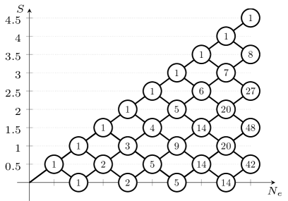
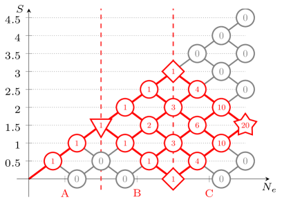
Figure 1: Left: Genealogical branching diagram in standard form for nine electrons. Right: Localising and site–ordering the orbitals expresses Hund’s rule on the first site and reduces the number of possible paths. Shown in red are the remaining non–vanishing CSFs with $S_{tot}=\frac{3}{2}$.

It was shown that for magnetic system described by Heisenberg–like models, further sparsity may be introduced into the graph, by taking advantage of the stabilisation arising from parallel alignment of site spins due to Hund’s rule.³³ Localising and site–ordering the orbitals makes the first three electrons correspond to site $A$, marked by a triangle in Figure 1, therefore non–Hund CSFs with $S_{A}\neq\frac{3}{2}$ get energetically penalised. This sparsity manifests in the Full CI expansion as well through a reduction of CSFs with appreciable weight.³³ It bears mentioning however, that Hund’s rule on sites $B$ and $C$ can not be expressed with a standard representation in most cases, since local spin quantum numbers corresponding to $B$ and $C$ are not defined in this basis. Collinear states with $S_{AB}=\{0,3\}$, marked by squares in Figure 1, are an exempt from this problem, since they can only follow from the coupling of two equal spins.

To mimic the local spin operators of the model, electrons on each site should be pre–coupled before combining them into a total spin:

$$\ket{L}=\ket{\bar{S}_{1}^{1}\ldots\bar{S}_{1}^{\text{A}}S_{\text{A+1}}^{\text{A+2}}\ldots S_{\text{A+1}}^{\text{A+B}}\bar{S}_{1}^{\text{A+B}}\ldots\bar{S}_{1}^{n}},\quad S_{A}\equiv\bar{S}_{1}^{A},\quad S_{B}\equiv S_{A+1}^{A+B},\quad S_{AB}\equiv\bar{S}_{1}^{A+B}.$$ (3)

Bars are used to distinguish quantum numbers occurring in both the standard and non–standard representation.

$\ket{C}$ and $\ket{L}$ constitute different coupling schemes that are related by a recoupling transformation:

$$\ket{L}=\sum_{C}\ket{C}\braket{C}{L},$$ (4)

which we express with the graphical method of spin algebra^{34, 35, 36} in the style of Wormer and Paldus.³⁷ As an aid to the reader, used ingredients of the graphical method are briefly recapitulated in Appendix A; a comprehensive introduction can be found in reference 37. The diagrammatic approach is not new to quantum chemistry and has already been applied to the study of Serber spin functions^{38, 39, 40, 41}, the optimal segmentation of two–electron operators in the GUGA⁴² or subduction coefficients for a general system partitioning $U(n=n_{1}+n_{2})=U(n_{1})\times U(n_{2})$^{43, 44} among others. Compared to previous work,^{43, 44} our derivation of the recoupling expressions is entirely inductive and does not rely on recursion. Although less general, this approach leads to simple closed formulas for systems with equal spins and we expect them to be convenient for studying other model Hamiltonians as well. Following the introductory example, the recoupling of two sites with three electrons into a local spin adapted representation, $S_{6}=S_{3}\times S_{3}$, will serve as the base case, before treating the general two site problem $S_{2n}=S_{n}\times S_{n}$ and the chain $S_{kn}=S_{n}\times(\ldots)_{k-2}\times S_{n}$. Afterwards, we illustrate with a protonated $\ce{[CaMn3^{(IV)}O4]}$ and an $\ce{[Fe^{(III)}4S4]}$ cubane how to use these expressions in practice.

Before $\braket{C}{L}$ is amenable to graphical manipulation, it has to be converted into a generalised Clebsch–Gordan coefficient. Inserting the resolution of the identity over all uncoupled states into equation (4), we obtain:

$$\ket{L}=\sum_{\ket{C}}\ket{C}\braket{C}{L}=\sum_{\ket{C}}\sum_{m_{s_{1}}\ldots m_{s_{k}}}\ket{C}\braket{C}{s_{1}m_{s_{1}}\ldots s_{k}m_{s_{k}}}\braket{s_{1}m_{s_{1}}\ldots s_{k}m_{s_{k}}}{L}$$ (5)

or graphically for $S_{6}=S_{3}\times S_{3}$:

$$\sum_{m_{s_{1}}\ldots m_{s_{k}}}\leavevmode\hbox to193.88pt{\vbox to136.05pt{\text{[drawing]}}} - - - - - + + + + + S_{1}^{5} S_{1}^{4} S_{1}^{3} S_{1}^{2} S_{4}^{5} S_{4}^{6} \bar{S}_{1}^{3} \bar{S}_{1}^{2} s_{4} s_{5} s_{2} s_{1} s_{3} s_{6} \bar{S}_{1}^{6} s_{1} s_{2} s_{3} s_{4} s_{5} s_{6} S_{1}^{6} - - - - - + + + + + S_{1}^{5} S_{1}^{4} S_{1}^{3} S_{1}^{2} S_{4}^{5} S_{4}^{6} \bar{S}_{1}^{3} \bar{S}_{1}^{2} s_{4} s_{5} s_{2} s_{1} s_{3} s_{6} \bar{S}_{1}^{6} s_{1} s_{2} s_{3} s_{4} s_{5} s_{6} S_{1}^{6}$$ (6)

Contracting over all magnetic quantum numbers and transitioning into 3–$jm$ symbols yields:

(7)

where the notation $[J_{1}J_{2}\ldots]=(2J_{1}+1)(2J_{2}+1)$ was introduced. To simplify the phase, we repeatedly use the relation $(-1)^{4J}=(-1)^{2(J_{1}+J_{2}+J_{12})}=1$. After a two line separation over $S_{1}^{3}$/$\bar{S}_{1}^{3}$, the arrow directions on $\bar{S}_{1}^{2}$ and $S_{4}^{5}$ are reversed:

(8)

Following another two line separation over $S_{1}^{2}$/$\bar{S}_{1}^{2}$ and a three line separation over $S_{4}^{5}$/$S_{1}^{3}$/$S_{1}^{5}$, the $6j$ symbols are brought into standard form, by changing the vertices and arrows marked in red:

(9)

where we used an identity of the type $(-1)^{2J_{12}+2J_{3}}=(-1)^{2J_{13}}$ twice. The genealogical CSFs $\ket{C}$ fulfil the triangle condition for cumulative spins by construction and the $3j$ symbols take the value one accordingly. Substituting $s_{i}=\frac{1}{2}$, using the symmetry of the $6j$ symbol under the column permutation $(123)\leftrightarrow(321)$ and flipping columns one and three, the recoupling coefficients $\braket{C}{L}$ for $S_{6}=S_{3}\times S_{3}$ take the form:

$$\begin{split}&\delta(S_{1}^{2},\bar{S}_{1}^{2})\delta(S_{1}^{3},\bar{S}_{1}^{3})\delta(S_{1}^{6},\bar{S}_{1}^{6})\times\\ &(-1)^{(S_{1}^{3}+S_{1}^{5}+1)+(S_{1}^{3}+\frac{1}{2}+S_{4}^{5}+S_{1}^{6})}\left[S_{1}^{4}S_{4}^{5};S_{1}^{5}S_{4}^{6}\right]^{1/2}\begin{Bmatrix}S_{1}^{5}&\frac{1}{2}&S_{1}^{4}\\[2.0pt] \frac{1}{2}&S_{1}^{3}&S_{4}^{5}\end{Bmatrix}\begin{Bmatrix}S_{1}^{6}&\frac{1}{2}&S_{1}^{5}\\[2.0pt] S_{4}^{5}&S_{1}^{3}&S_{4}^{6}\end{Bmatrix}\end{split}.$$ (10)

If we introduce the weighted symbol $\widetilde{W}$ related to the original Racah coefficient $\overline{W}$⁴⁵:

$$\widetilde{W}\begin{pmatrix}j_{1}&j_{2}&J_{12}\\ j_{3}&J&J_{23}\end{pmatrix} =[J_{12}J_{23}]^{1/2}\overline{W}\begin{pmatrix}j_{1}&j_{2}&J_{12}\\ j_{3}&J&J_{23}\end{pmatrix}$$ (11)

$$=[J_{12}J_{23}]^{1/2}(-1)^{j_{1}+j_{2}+j_{3}+J}\begin{Bmatrix}j_{1}&j_{2}&J_{12}\\ j_{3}&J&J_{23}\end{Bmatrix},$$

we can write equation (10) compactly as:

$$\delta(S_{1}^{2},\bar{S}_{1}^{2})\delta(S_{1}^{3},\bar{S}_{1}^{3})\delta(S_{1}^{6},\bar{S}_{1}^{6})\text{ }\widetilde{W}\begin{pmatrix}S_{1}^{5}&\frac{1}{2}&S_{1}^{4}\\[2.0pt] \frac{1}{2}&S_{1}^{3}&S_{4}^{5}\end{pmatrix}\widetilde{W}\begin{pmatrix}S_{1}^{6}&\frac{1}{2}&S_{1}^{5}\\[2.0pt] S_{4}^{5}&S_{1}^{3}&S_{4}^{6}\end{pmatrix}.$$ (12)

Equation (12) may be generalised to the case of $k$ sites with $S_{i}=\frac{3}{2}$. Due to the local spin coupling scheme, different sites remain separable over two lines, entirely similar to $S_{1}^{3}$ / $\bar{S}_{1}^{3}$ in equation (10) and introduce a factor analogous to (11) with a constant offset:

$$\begin{split}\delta(S_{1}^{2},\bar{S}_{1}^{2})\delta(S_{1}^{3k},\bar{S}_{1}^{3k})\prod_{i=0}^{k-2}\delta(S_{1}^{3+3i},\bar{S}_{1}^{3+3i})\widetilde{W}\begin{pmatrix}S_{1}^{5+3i}&\frac{1}{2}&S_{1}^{4+3i}\\[2.0pt] \frac{1}{2}&S_{1}^{3+3i}&S_{4+3i}^{5+3i}\end{pmatrix}\widetilde{W}\begin{pmatrix}S_{1}^{6+3i}&\frac{1}{2}&S_{1}^{5+3i}\\[2.0pt] S_{4+3i}^{5+3i}&S_{1}^{3+3i}&S_{4+3i}^{6+3i}\end{pmatrix}.\end{split}$$ (13)

To generalise to arbitrary spins $S_{n}$, it is instructive to first observe the action of adding one electron to each of two sites, as in $S_{8}=S_{4}\times S_{4}$ (phases and factors omitted):

(14)

Compared to (8), an additional $3j$ symbol can be factored out from the left drawing and two extra vertices are formed on the right. After separating over three lines twice, $S_{1}^{4}/S_{4}^{6}/S_{1}^{6}$ and $S_{1}^{4}/S_{4}^{7}/S_{1}^{7}$, the right hand side reduces to a product of three $6j$ symbols, i.e. every additional electron contributes one $6j$ coefficient per site. Taking the phases into account as previously, the recoupling coefficient for $S_{2n}=S_{n}\times S_{n}$ becomes a product of $\widetilde{W}$ over site electrons $n$:

$$\prod_{p=2}^{n-1}\delta(S_{1}^{p},\bar{S}_{1}^{p})\times\delta(S_{1}^{n},\bar{S}_{1}^{n})\delta(S_{1}^{2n},\bar{S}_{1}^{2n})\prod_{m=0}^{n-2}\widetilde{W}\begin{pmatrix}S_{1}^{2+m+n}&\frac{1}{2}&S_{1}^{1+m+n}\\[2.0pt] S_{1+n}^{1+m+n}&S_{1}^{n}&S_{1+n}^{2+m+n}\end{pmatrix}.$$ (15)

The general expression for recoupling a chain of equivalent spins $S_{i}\geq 1$ into $S_{kn}=S_{n}\times(\ldots)_{k-2}\times S_{n}$ is a combination of equations (13) and (15). Every site adds another $2n$ vertices to the graph, yielding $(n-1)$ $6j$ symbols. In total the recoupling coefficient is a product of $(k-1)(n-1)$ Racah coefficients with the corresponding Kronecker deltas:

$$\begin{split}\braket{C}{L}=&\prod_{p=2}^{n-1}\delta(S_{1}^{p},\bar{S}_{1}^{p})\times\delta(S_{1}^{kn},\bar{S}_{1}^{kn})\times\\ &\prod_{i=0}^{k-2}\prod_{m=0}^{n-2}\delta(S_{1}^{n(i+1)},\bar{S}_{1}^{n(i+1)})\widetilde{W}\begin{pmatrix}S_{1}^{2+m+n(i+1)}&\frac{1}{2}&S_{1}^{1+m+n(i+1)}\\[2.0pt] S_{1+n(i+1)}^{1+m+n(i+1)}&S_{1}^{n(i+1)}&S_{1+n(i+1)}^{2+m+n(i+1)}\end{pmatrix}.\end{split}$$ (16)

3 Application: [CaMn^(IV)3O4] Cubane

The [CaMn^(IV)3O4] cubane shown in Figure 2 is inspired by a synthetic model of the oxygen evolving complex of photosystem II. Compared to the experimental structure,⁴⁶ the ligands were simplified and the bridging oxygen in the Mn_A Mn_B plane protonated,⁴⁷ to study the impact of oxo–protonation on the electronic structure.

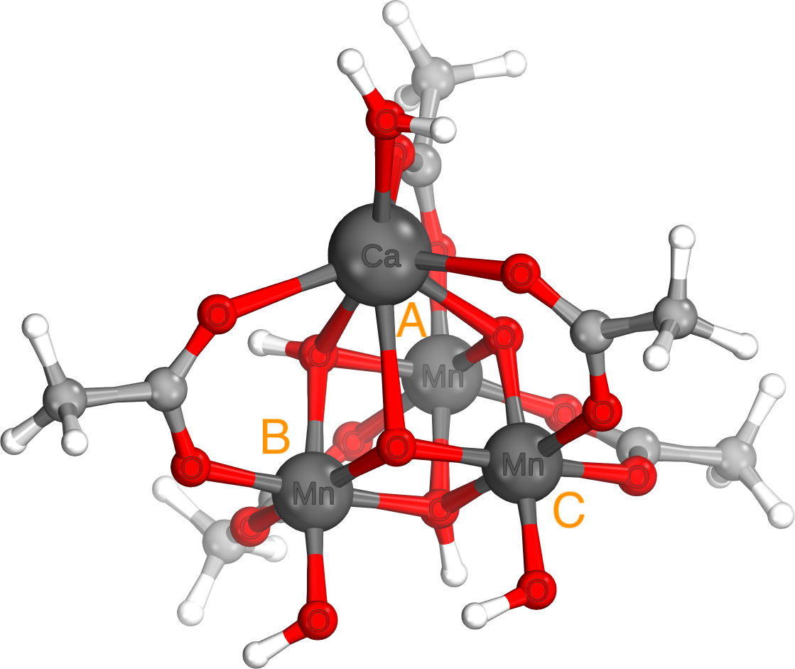
Figure 2: Geometry of the doubly protonated [CaMn^(IV)3O4] cubane model.⁴⁷ Magnetic sites are labelled $A,B,C$ following equation (17). The picture was created with IboView.^{48, 49}

In the original study on this compound,⁴⁷ broken–symmetry (BS) DFT calculations assuming an isotropic, three–parameter Heisenberg model:

$$\hat{\mathcal{H}}_{3J}=\sum_{i<j}^{\{A,B,C\}}J_{ij}(\hat{S}_{i}\cdot\hat{S}_{j}),$$ (17)

predicted an octet ground state with couplings constants $J_{AB}=$6.2\text{\,}{\mathrm{cm}}^{-1}$$, $J_{AC}=$-40.2\text{\,}{\mathrm{cm}}^{-1}$$ and $J_{BC}=$-25.4\text{\,}{\mathrm{cm}}^{-1}$$. Experimental estimates for this structure are not available. With three distinct coupling, equation (17) is no longer analytically solvable, making it an interesting target for the effective Hamiltonian approach. Another advantage of the effective Hamiltonians is the straightforward incorporation of higher–order interactions and in the following we consider a more general expression including biquadratic interactions $K_{ij}(\hat{S}_{i}\cdot\hat{S}_{j})^{2}$, denoted $\hat{\mathcal{H}}_{3J3K}$, see also section S3 in the supporting information.

Apart from the extra recoupling step described in the previous section, formation of the effective Hamiltonian follows the standard prescription,^{50, 20, 21} i.e. (i) obtain the CI vector in the standard CSF basis, (ii) transform relevant CSFs into the required coupling scheme, (iii) project onto the model space, ensuring that the discarded norm is small, (iv) orthonormalise the projections and (v) invert the spectral decomposition with the ab–initio energies. Magnetic couplings can then be obtained from a mean–square fit of the numerical to the analytical matrix. In the first step, the phase convention of the CI vector should be accounted for. Recoupling CSFs in the unitary group formalism, as for instance used in OpenMolcas,⁵¹ requires a phase to be applied beforehand:^{52, 53}

$$\phi=(-1)^{2\left(\sum_{k\in\{l_{23}\}}S_{1}^{k-1}\right)},$$ (18)

where $\{l_{23}\}$ denotes level indices with values 2 or 3 (negative coupling or doubly occupied) in UGA $\mathbf{d}$ vector notation.⁵² In line with the introductory example, the $S_{\text{tot}}=\frac{3}{2}$ block of the model matrix is shown in Table 1. The remaining blocks are given in the supporting information.

Table 1: Analytical matrix corresponding to $\hat{\mathcal{H}}_{3J3K}$ in the basis $\ket{S_{tot}=\frac{3}{2},S_{AB}}$. Zero matrix elements were omitted for clarity. We made the substitutions $J_{3m}=J_{13}-J_{23}$, $J_{3p}=J_{13}+J_{23}$ and analogously for $K_{3m}$ and $K_{3p}$, to make clear that setting $J_{13}=J_{23}$ and $K_{ij}=0$ diagonalises the model.^{54, 55}

$\hat{\mathcal{H}}_{3J3K}$	$\ket{\frac{3}{2},0}$	$\ket{\frac{3}{2},1}$
$\bra{\frac{3}{2},0}$	$-\frac{15}{16}(4J_{12}+5(3K_{12}+K_{3p}))$	$-\frac{5}{8}\sqrt{3}(2J_{3m}+K_{3m})$
$\bra{\frac{3}{2},1}$	$-\frac{5}{8}\sqrt{3}(2J_{3m}+K_{3m})$	$\frac{1}{80}(-5(44J_{12}+8J_{3p}+121K_{12})-587K_{3p})$
$\bra{\frac{3}{2},2}$	$-\frac{3\sqrt{5}K_{3p}}{2}$	$-2\sqrt{\frac{3}{5}}(J_{3m}+2K_{3m})$
$\bra{\frac{3}{2},3}$		$-\frac{3\sqrt{21}K_{3p}}{10}$
$\hat{\mathcal{H}}_{3J3K}$	$\ket{\frac{3}{2},2}$	$\ket{\frac{3}{2},3}$
$\bra{\frac{3}{2},0}$	$-\frac{3\sqrt{5}K_{3p}}{2}$
$\bra{\frac{3}{2},1}$	$-2\sqrt{\frac{3}{5}}(J_{3m}+2K_{3m})$	$-\frac{3\sqrt{21}K_{3p}}{10}$
$\bra{\frac{3}{2},2}$	$-\frac{3}{16}(4J_{12}+8J_{3p}+3K_{12}+29K_{3p})$	$-\frac{3}{8}\sqrt{\frac{7}{5}}(2J_{3m}+9K_{3m})$
$\bra{\frac{3}{2},3}$	$-\frac{3}{8}\sqrt{\frac{7}{5}}(2J_{3m}+9K_{3m})$	$\frac{9J_{12}}{4}-3J_{3p}-\frac{27}{80}(15K_{12}+29K_{3p})$

The corresponding numerical matrices were derived from calculations performed with OpenMolcas⁵¹ using the ANO–RCC basis set⁵⁶ of double–$\zeta$ quality with contractions Ca(20s16p)/[5s4p], Mn(21s15p10d)/[5s4p2d], O(14s9p)/[3s2p], C(14s9p)/[2s1p], H(8s)/[1s] and the Cholesky decomposition of two–electron integrals with a threshold of $1\text{\times}{10}^{-4}\text{\,}$.^{57, 58}

A minimal description of the magnetic interactions is achieved by correlating the nine electrons occupying the $t_{2g}$ orbitals in a CAS(9,9). Spin models usually assume a common spatial component, hence state–averaged CASSCF over the ground state of every multiplicity in equation (1) with equal weight was performed. The $S_{\text{tot}}=\frac{3}{2}$ block of the numerical matrix is shown in Table 2; all other blocks can be found in the supporting information.

Table 2: Effective Hamiltonian obtained from CASSCF(9,9) with column labels $\ket{S_{\text{total}}=\frac{3}{2},S_{AB}}$ relative to $E(S_{\text{total}}=\frac{9}{2})$ in units of $\text{\,}{\mathrm{cm}}^{-1}$. Zeros were omitted to enhance legibility.

$\hat{\mathcal{H}}_{\mathrm{eff}}^{\mathrm{CASSCF}}$	$\ket{\frac{3}{2},0}$	$\ket{\frac{3}{2},1}$	$\ket{\frac{3}{2},2}$	$\ket{\frac{3}{2},3}$
$\bra{\frac{3}{2},0}$	147	17
$\bra{\frac{3}{2},1}$	17	165	12
$\bra{\frac{3}{2},2}$		12	199	7
$\bra{\frac{3}{2},3}$			7	251

Interactions constants are all ferromagnetic at this level of theory and sufficiently different to warrant a 3$J$ model, see the second row of Table 4. It is known that minimal CASSCF magnetic orbitals are too localised on the metals as a consequence of the mean field description of virtual ligand–to–metal charge transfer.⁵⁹ Rather than trying to capture this interaction perturbatively, we expand the variational space within the restricted active space (RAS) framework to keep exact diagonalisation feasible.⁶⁰ Six unprotonated bridging O $2p$ and three $\sigma_{\text{Mn-O}}$ were added to RAS1 and six empty Mn $e_{g}$ orbitals to RAS3, with up to two holes and particles, respectively, which we abbreviate as RAS(27,24). Orbital pictures are provided in the supporting information. These active orbitals are expected to make the largest differential contributions to the superexchange mechanism and prevent some of the Mn $e_{g}$ to be rotated out in favour of O $p^{\prime}$ orbitals. Analogous to the smaller CAS(9,9), a state–averaged RASSCF over the ground state of each spin sector was performed. Correlating the ligands introduces delocalisation tails into the metal–centred orbitals and reduces the retained wave function norm after projection onto the model space to $\approx 78\%$. This number may appear small, but a reduced weight of the magnetic manifold is to be expected with an increasing ligand–to–metal charge transfer in the extended active space. The RAS retains a dectet ground state, but compresses the gaps between states, as can be seen for the quartet block in Table 3. All remaining spin sectors are given in the supporting information.

Table 3: Effective Hamiltonian obtained from RASSCF(27, 24) with column labels $\ket{S_{\text{total}}=\frac{3}{2},S_{AB}}$ relative to $E(S_{\text{total}}=\frac{9}{2})$ in units of $\text{\,}{\mathrm{cm}}^{-1}$. Zeros were omitted to enhance legibility.

$\hat{\mathcal{H}}_{\mathrm{eff}}^{\mathrm{RASSCF}}$	$\ket{\frac{3}{2},0}$	$\ket{\frac{3}{2},1}$	$\ket{\frac{3}{2},2}$	$\ket{\frac{3}{2},3}$
$\bra{\frac{3}{2},0}$	79	40
$\bra{\frac{3}{2},1}$	40	89	28
$\bra{\frac{3}{2},2}$		28	107	16
$\bra{\frac{3}{2},3}$			16	136

In contrast to the minimal CAS, the coupling constants from RASSCF, listed in the third row of Table 4, indicate an almost symmetric interaction between Mn_A/Mn_C and Mn_B/Mn_C. Biquadratic contributions remain negligible, supporting the simplified model employed in reference 47.

With an improved reference wave function, it makes sense to also consider dynamic correlation effects outside the active space. Here we settled for multi–configurational pair density functional theory (MCPDFT),^{61, 62, 63} due to its favourable cost–to–performance ratio compared to RASPT2.⁶⁴ Notably, the tested functionals consistently predict a sextet ground state with purely antiferromagnetic couplings while maintaining symmetric $J_{12}/J_{23}$ exchange pathways, as shown in the last three rows of Table 4. Couplings obtained with the SCAN–E0⁶⁵ functional are more than twice as large as those from PBE^{66, 67} or BLYP^{68, 69, 70}, but display the same qualitative trend. Considering excitation level restrictions of the RASSCF and basis set limitations, our estimates are unlikely to be converged. Full CASSCF calculations are required to understand the discrepancy between the BS–DFT and RASSCF+MCPDFT results, which will be subject of future work.

Table 4: Magnetic coupling constants in units of $\text{\,}{\mathrm{cm}}^{-1}$ derived from CASSCF(9,9) and different fully translated pair density functionals with a RASSCF(27, 24) reference wave function, as well as the BS–DFT estimate from reference 47.

	$J_{12}$	$J_{13}$	$J_{23}$	$K_{12}$	$K_{13}$	$K_{23}$
BS–DFT47	6.2	-40.2	-25.4	–	–	–
CASSCF(9, 9)	-6.6	-27.7	-20.0	0.0	0.0	0.0
RASSCF(27, 24)	-3.5	-22.2	-3.7	0.0	0.0	-0.1
+MCPDFT(ftPBE)	19.8	5.8	19.8	-0.1	0.3	-0.3
+MCPDFT(ftBLYP)	21.9	7.9	21.9	-0.1	0.3	-0.3
+MCPDFT(ftSCAN–E0)	54.0	23.4	53.9	-0.3	0.5	-0.6

4 Non–Sequential Coupling Patterns

Many transition metal clusters like the oxygen evolving complex or FeMo cofactor are formed by four or more magnetic sites. The sequential coupling of local spins implied by equation (16) will suffice to construct the effective Hamiltonian for these compounds, but it is known that certain models admit diagonal form in non–sequential orderings. A relevant example is the four site bilinear Heisenberg model:

$$\hat{\mathcal{H}}_{4J}=\sum_{i<j}^{\{A,B,C,D\}}J_{ij}(\hat{S}_{i}\cdot\hat{S}_{j}),\quad S_{A}=S_{B}=S_{C}=S_{D}$$ (19)

which is diagonal in the $((AB)(CD))$ coupling scheme.⁷¹ Drawn as a spin graph, see Figure 3, this arrangement of spins reminds of a balanced binary tree and thus the abbreviation

$$\ket{T}=\ket{\ldots\bar{S}_{1}^{\text{A}}\ldots S_{\text{A+1}}^{\text{B}}\bar{S}_{1}^{\text{A+B}}\ldots S_{\text{A+B+1}}^{\text{C}}\ldots S_{\text{C+1}}^{\text{D}}\ldots S_{\text{A+B+1}}^{\text{C+D}}\bar{S}_{\text{1}}^{\text{{A+B+C+D}}}}$$ (20)

will be used for these CSFs.

Figure 3: Coupling of four angular momenta in the $((AB)(CD))$ scheme, closely resembling a binary tree.

Local spins $A,B,C,D$ are already defined for $\ket{L}$ CSFs, hence the remaining transformation from (16), $(((AB)C)D)\rightarrow((AB)(CD))$, can be expressed as a single Racah coefficient:

$$\braket{L}{T}=\widetilde{W}\begin{pmatrix}S_{\text{AB}}&S_{\text{C}}&S_{\text{ABC}}\\ S_{\text{tot}}&S_{\text{D}}&S_{\text{CD}}\end{pmatrix},$$ (21)

allowing us to examine the properties of the ab–initio wave function in this basis. As an example, an all–ferric [Fe^(III)4S4(SMe)4] cubane model system will be considered.^{72, 32} The singlet manifold of this particular cluster was previously studied with GUGA–FCIQMC³². To illustrate the concept, we concentrate on the exactly diagonalisable $S_{\text{tot}}=8$ block of the minimal CAS(20,20) comprising the iron $3d$ orbitals. Calculations were performed with OpenMolcas⁵¹ using the ANO–RCC basis set⁵⁶ of double–$\zeta$ quality with contractions Fe(21s15p10d)/[5s4p2d], S(17s12p)/[4s3p], C(14s9p)/[2s1p], H(8s)/[1s] and the Cholesky decomposition of two–electron integrals with a threshold of $1\text{\times}{10}^{-4}\text{\,}$.^{57, 58}

The pertinent model space is spanned by six states, resulting from the coupling of four $S_{i}=\frac{5}{2}$. From the branching diagram, 170 open–shell CSFs can be identified in a localised basis, entirely similar to the left side of Figure 1. Table 5 lists the $L_{1}$ norm, $1\leq\sum_{i}^{n_{CSF}}|c_{i}|\leq\sqrt{n_{CSF}}$, and inverse participation ratio (IPR), $\frac{1}{n_{CSF}}\leq\sum_{i}^{n_{CSF}}c_{i}^{4}\leq 1$, as measures of sparsity in this generic basis $\ket{G}$ and compares it to the standard $\ket{C}$, local sequential $\ket{L}$ and binary tree $\ket{T}$ coupling schemes in the site–ordered basis. Assuming the worst–case scenario, orbitals in $\ket{G}$ are ordered such that electrons one and two are on different atoms, preventing partial fulfilment of Hund’s rule on the first site.

Table 5: Sparsity measures for the branching diagram CSFs of the first six roots $\ket{S_{tot}=8}$ in the singly occupied manifold $\ket{\bar{\psi}}$ of the CAS(20,20). Small values of the $L_{1}$ norm and large IPRs indicate sparse wave functions.

$S_{\text{tot}}=8$	$\ket{\bar{\psi}_{1}}$	$\ket{\bar{\psi}_{2}}$	$\ket{\bar{\psi}_{3}}$	$\ket{\bar{\psi}_{4}}$	$\ket{\bar{\psi}_{5}}$	$\ket{\bar{\psi}_{6}}$
$L_{1}$ norm
$\ket{G}$	10.4	10.3	10.3	11.4	7.86	10.4
$\ket{C}$	6.80	6.76	6.70	5.82	6.80	6.45
$\ket{L}$	1.46	1.97	1.96	1.72	1.46	1.69
$\ket{T}$	1.07	1.48	1.48	1.06	1.06	1.04
IPR
$\ket{G}$	0.01	0.01	0.01	0.01	0.03	0.01
$\ket{C}$	0.03	0.04	0.04	0.04	0.03	0.03
$\ket{L}$	0.56	0.33	0.34	0.4	0.56	0.41
$\ket{T}$	0.97	0.49	0.49	0.97	0.97	0.98

Enforcing Hund’s rule on the first site with the standard representation $\ket{C}$ reduces the number of appreciable CI coefficients from 170 to 50 and is accompanied by a significant increase in sparsity as quantified by the $L_{1}$ criterion. The increase in IPR is much smaller, because strong mixing within this reduced space still is necessary to resolve Hund’s rule on sites $B$, $C$ and $D$. Proceeding to $\ket{L}$ and $\ket{T}$, only six non–vanishing CSFs remain and their squared coefficients are shown in Table 6.

Table 6: Weights of wave functions for the first six $S_{tot}=8$ roots of the CAS(20,20) projected onto the Heisenberg manifold in the local sequential and balanced binary tree coupling schemes. Zeros were omitted to enhance legibility. Since roots two and three and four and five are (nearly) degenerate, mixing within the relevant subspaces is possible.

$S_{\text{tot}}=8$	$\ket{\bar{\psi}_{1}}$	$\ket{\bar{\psi}_{2}}$	$\ket{\bar{\psi}_{3}}$	$\ket{\bar{\psi}_{4}}$	$\ket{\bar{\psi}_{5}}$	$\ket{\bar{\psi}_{6}}$
$\Delta E$ / $\text{\,}{\mathrm{cm}}^{-1}$	0	14	16	76	76	157
$\ket{L}=\ket{S_{AB},S_{ABC}}$
$\ket{3,\frac{11}{2}}$		0.48	0.50
$\ket{4,\frac{11}{2}}$	0.30				0.68
$\ket{4,\frac{13}{2}}$	0.68				0.30
$\ket{5,\frac{11}{2}}$		0.07	0.07	0.44		0.41
$\ket{5,\frac{13}{2}}$		0.21	0.20	0.10		0.48
$\ket{5,\frac{15}{2}}$		0.23	0.22	0.45		0.09
$\ket{T}=\ket{S_{AB},S_{CD}}$
$\ket{3,5}$		0.48	0.50
$\ket{4,4}$	0.99
$\ket{4,5}$					0.99
$\ket{5,3}$		0.50	0.48
$\ket{5,4}$				0.99
$\ket{5,5}$						0.99

Although sparsity is maximised in $\ket{T}$, as would be expected from equation (19), the largest gain is already realised by recoupling from $\ket{C}$ to $\ket{L}$, where Hund’s rule can be expressed on every site. This example makes a case in point for the $\ket{L}$ basis, because the redox cycles in nature mostly feature metal centres of mixed oxidation states for which $\ket{T}$ CSFs are not expected to be more descriptive. Nevertheless, we presume that non–sequential couplings could be advantageous for partitioning large magnetic systems into smaller units whenever the subsystem exhibits a particular symmetry, e.g. treating the FeMo cofactor in terms of two magnetically coupled cuboids.

5 Conclusion

In this communication, we extended the effective Hamiltonian formalism to polynuclear transition metal complexes with local spins greater than one half by means of recoupling transformations. The method was used to assess a spin model for a [CaMn^(IV)3O4] cubane with minimal and extended active space calculations. Enlarging the active was shown to qualitatively change the magnetism from a three parameter to a two parameter interaction, illustrating the utility and importance of an exact mapping between ab–initio and model wave functions. An extension to sparse solvers like DMRG or FCIQMC is readily possible, if CI coefficients can be efficiently extracted. We also discussed how chains of local–spin–adapted functions can be transformed into non–sequential, tree–like orderings to express additional permutational symmetries of model Hamiltonians in ab–initio wave functions. Overall, the increased compactness of CI solutions in non–standard coupling schemes portends a promising future for their use in sparse solvers like FCIQMC or as reference states for perturbation theory. It remains to be seen whether the additional sparsity compared to the standard basis outweighs the overhead of more complicated Hamiltonian matrix element evaluation.^{73, 74}

Appendix A. Recapitulation of Angular Momentum Diagrams

Clebsch–Gordan coefficients, $\braket{j_{1}m_{1};j_{2}m_{2}}{j_{3}m_{3}}$, are the building blocks of the Racah–Wigner calculus. The angular momenta fulfil the triangle condition:

$$\begin{split}|j_{1}-j_{2}|\leq j_{3}\leq j_{1}+j_{2}\end{split}$$ (22)

and sum to an integer $j_{1}+j_{2}+j_{3}\in\mathbb{Z}^{0\leq}$. In graphical notation, they are represented by three lines connected to a half circle vertex. Standard and contrastandard states are denoted by single and double arrows, respectively. SU(2) invariants are formed by summing over all magnetic quantum numbers of a standard/contrastandard product. Since bra/ket and ket/bra contractions are invariant under simultaneous time–reversal, these contracted lines are not oriented, see also equations (54) and (55) in reference 37. Note that coupling more than two angular momenta implies a summation over the magnetic quantum numbers of intermediate $j$, e.g.:

$$\braket{j_{1}m_{1};j_{2}m_{2};j_{3}m_{3}}{((j_{1}j_{2})j_{3})jm}=\sum_{m_{j_{12}}}\braket{j_{1}m_{1};j_{2}m_{2}}{j_{12}m_{12}}\braket{j_{12}m_{12};j_{3}m_{3}}{jm}.$$ (23)

Whereas recoupling problems are conveniently expressed in terms of generalised Clebsch–Gordan coefficients, owing to their cumbersome symmetries, it is convenient for the diagrammatic approach to use more symmetric 3–$jm$ symbols instead. Following chapter 3.6 of reference 37, this conversion involves five steps (always referring to the initial diagram):³⁷

1. change the sign of the vertex,

2. keeping their direction, exchange all double arrows with single arrows,

3. add a factor $\sqrt{2j+1}$ for the unique line, i.e. the line of bra or ket type appearing only once,

4. add a factor $(-1)^{2j}$ for the first line encountered in going from the unique single (ket)/double (bra) arrow line into the direction indicated by the vertex sign (for a ket: $-$ clockwise / $+$ counter clockwise, for a bra: $-$ counter clockwise / $+$ clockwise),

5. add a factor $(-1)^{2j}$ for every time–reversed bra (outgoing double arrow).

For example:

$$\braket{\theta(j_{3}m_{3})}{j_{1}m_{1}\text{; }j_{2}m_{2}}=(-1)^{2j_{2}+2j_{3}}\sqrt{2j_{3}+1}\begin{pmatrix}j_{1}&j_{3}&j_{2}\\ m_{1}&m_{3}&m_{2}\end{pmatrix}$$ (24)

Changing the node sign on a 3–$jm$ symbol, corresponding to an odd permutation of columns, incurs a factor of $(-1)^{j_{1}+j_{2}+j_{3}}$. Unlike the bra/ket and ket/bra contractions of Clebsch–Gordan coefficients, the lines of contracted 3–$jm$ symbols are oriented. Arrows on contracted lines can be inverted, introducing a factor of $(-1)^{2j}$. A diagram with two external lines can be closed as follows:

From a contracted graph, a sequence of line separations leads to irreducible 3$n$–$j$ symbols. In the main text, we use the two and three line separation theorems:

Closed and open boxes represent diagrams with fully and non–contracted lines, respectively.

The final expressions are written in terms of $3j$ and $6j$ symbols, the former of which is defined as:

$$\begin{Bmatrix}j_{1}&j_{2}&j_{3}\end{Bmatrix}=\begin{cases}1,&\text{for }|j_{1}-j_{2}|\leq j_{3}\leq j_{1}+j_{2}\\ 0,&\text{else}.\end{cases}$$ (25)

The $6j$ symbol is a contraction of four 3–$jm$ symbols:

$$\begin{Bmatrix}j_{1}&j_{2}&j_{3}\\ j_{4}&j_{5}&j_{6}\end{Bmatrix}$$ (26)

In standard form, all vertices have the same sign. The inner lines either all point towards or away from the centre, whereas the outer arrows follow the direction indicated by the vertex sign. Inverting all signs and outer arrow directions is equivalent to reflecting the symbol on an outer axis. Arbitrary column permutations or the pairwise inversion of bottom and top elements leave the $6j$ symbol invariant, e.g.:

$$\begin{Bmatrix}j_{1}&j_{2}&j_{3}\\ j_{4}&j_{5}&j_{6}\end{Bmatrix}=\begin{Bmatrix}j_{6}&j_{2}&j_{4}\\ j_{3}&j_{5}&j_{1}\end{Bmatrix}.$$ (27)

Many programming languages provide optimised libraries or wrappers to obtain the numerical values of 3–$nj$ symbols.⁷⁵

Funding was provided by the Max Planck Society. N. A. Bogdanov thanks Huanchen Zhai for discussions on how to extract CI coefficients from MPS wave functions.

References

- Caneschi et al. 1991 Caneschi, A.; Gatteschi, D.; Sessoli, R.; Barra, A. L.; Brunel, L. C.; Guillot, M. Journal of the American Chemical Society 1991, 113, 5873–5874
- Sessoli et al. 1993 Sessoli, R.; Gatteschi, D.; Caneschi, A.; Novak, M. A. Nature 1993, 365, 141–143
- Chibotaru 2023 Chibotaru, L. F. Computational Modelling of Molecular Nanomagnets; Springer International Publishing, 2023; pp 1–62
- Lee and Ogawa 2017 Lee, S.; Ogawa, T. Chemistry Letters 2017, 46, 10–18
- Titiš et al. 2023 Titiš, J.; Rajnák, C.; Boča, R. Inorganics 2023, 11, 452
- Bogani and Wernsdorfer 2008 Bogani, L.; Wernsdorfer, W. Nature Materials 2008, 7, 179–186
- Rinehart et al. 2011 Rinehart, J. D.; Fang, M.; Evans, W. J.; Long, J. R. Journal of the American Chemical Society 2011, 133, 14236–14239
- Guo et al. 2024 Guo, Y.; He, L.; Ding, Y.; Kloo, L.; Pantazis, D. A.; Messinger, J.; Sun, L. Nature Communications 2024, 15
- Pámies and Bäckvall 2003 Pámies, O.; Bäckvall, J.-E. Chemical Reviews 2003, 103, 3247–3262
- Köhler et al. 2012 Köhler, V. et al. Nature Chemistry 2012, 5, 93–99
- Wang et al. 2013 Wang, Z. J.; Clary, K. N.; Bergman, R. G.; Raymond, K. N.; Toste, F. D. Nature Chemistry 2013, 5, 100–103
- Li et al. 2019 Li, D.; Lee, K.; Wang, B. Y.; Osada, M.; Crossley, S.; Lee, H. R.; Cui, Y.; Hikita, Y.; Hwang, H. Y. Nature 2019, 572, 624–627
- Takahashi et al. 2008 Takahashi, H.; Igawa, K.; Arii, K.; Kamihara, Y.; Hirano, M.; Hosono, H. Nature 2008, 453, 376–378
- Bednorz and Müller 1986 Bednorz, J. G.; Müller, K. A. Zeitschrift für Physik B Condensed Matter 1986, 64, 189–193
- Lee et al. 2006 Lee, P. A.; Nagaosa, N.; Wen, X.-G. Reviews of Modern Physics 2006, 78, 17–85
- Sharma and Chan 2012 Sharma, S.; Chan, G. K.-L. The Journal of Chemical Physics 2012, 136
- Dobrautz et al. 2021 Dobrautz, W.; Weser, O.; Bogdanov, N. A.; Alavi, A.; Li Manni, G. Journal of Chemical Theory and Computation 2021, 17, 5684–5703
- Griffith 1960 Griffith, J. Molecular Physics 1960, 3, 79–89
- McWeeny 1965 McWeeny, R. The Journal of Chemical Physics 1965, 42, 1717–1725
- Malrieu et al. 2013 Malrieu, J. P.; Caballol, R.; Calzado, C. J.; de Graaf, C.; Guihéry, N. Chemical Reviews 2013, 114, 429–492
- Maurice et al. 2009 Maurice, R.; Bastardis, R.; Graaf, C. d.; Suaud, N.; Mallah, T.; Guihiéry, N. Journal of Chemical Theory and Computation 2009, 5, 2977–2984
- Shavitt 1981 Shavitt, I. The Unitary Group for the Evaluation of Electronic Energy Matrix Elements; Springer Berlin Heidelberg, 1981; p 51–99
- Duch and Karwowski 1985 Duch, W.; Karwowski, J. Computer Physics Reports 1985, 2, 93–170
- Matsen 1964 Matsen, F. A. Advances in Quantum Chemistry 1964, 1, 59–114
- Kaplan 2013 Kaplan, I. G. Symmetry of Many-Electron Systems: Physical Chemistry: A Series of Monographs; Academic Press, 2013; Vol. 34
- Keller and Reiher 2016 Keller, S.; Reiher, M. The Journal of Chemical Physics 2016, 144
- Wouters et al. 2014 Wouters, S.; Poelmans, W.; Ayers, P. W.; Van Neck, D. Computer Physics Communications 2014, 185, 1501–1514
- Dobrautz et al. 2019 Dobrautz, W.; Smart, S. D.; Alavi, A. The Journal of Chemical Physics 2019, 151, 094104
- Han et al. 2023 Han, R.; Luber, S.; Li Manni, G. Journal of Chemical Theory and Computation 2023, 19, 2811–2826
- Kurashige et al. 2013 Kurashige, Y.; Chan, G. K.-L.; Yanai, T. Nature Chemistry 2013, 5, 660–666
- Sharma et al. 2014 Sharma, S.; Sivalingam, K.; Neese, F.; Chan, G. K.-L. Nature Chemistry 2014, 6, 927–933
- Li Manni et al. 2021 Li Manni, G.; Dobrautz, W.; Bogdanov, N. A.; Guther, K.; Alavi, A. The Journal of Physical Chemistry A 2021, 125, 4727–4740
- Li Manni et al. 2020 Li Manni, G.; Dobrautz, W.; Alavi, A. Journal of Chemical Theory and Computation 2020, 16, 2202–2215
- Jucys et al. 1962 Jucys, A.; Levinson, I. B.; Vanagas, V. V. Mathematical apparatus of the theory of angular momentum; Israel Program for Scientific Translations, 1962
- Varshalovich et al. 1988 Varshalovich, D.; Moskalev, A.; Khersonskii, V. K. Quantum theory of angular momentum; World Scientific, 1988
- Balcar and Lovesey 2009 Balcar, E.; Lovesey, S. W. Introduction to the Graphical Theory of Angular Momentum: Case Studies; Springer Berlin Heidelberg, 2009
- Wormer and Paldus 2006 Wormer, P. E.; Paldus, J. Advances in Quantum Chemistry; Elsevier, 2006; pp 59–123
- Wilson 1977 Wilson, S. Chemical Physics Letters 1977, 49, 168–173
- Wormer and Paldus 1980 Wormer, P. E. S.; Paldus, J. International Journal of Quantum Chemistry 1980, 18, 841–866
- Paldus and Wormer 1979 Paldus, J.; Wormer, P. E. S. International Journal of Quantum Chemistry 1979, 16, 1321–1335
- Paldus and Wormer 1978 Paldus, J.; Wormer, P. E. S. Physical Review A 1978, 18, 827–840
- Paldus and Boyle 1980 Paldus, J.; Boyle, M. J. Physica Scripta 1980, 21, 295–311
- Zhenyi 1986 Zhenyi, W. International Journal of Quantum Chemistry 1986, 29, 1779–1787
- Wen 1993 Wen, Z. International Journal of Quantum Chemistry 1993, 48, 303–308
- Racah 1942 Racah, G. Physical Review 1942, 62, 438–462
- Mukherjee et al. 2012 Mukherjee, S.; Stull, J. A.; Yano, J.; Stamatatos, T. C.; Pringouri, K.; Stich, T. A.; Abboud, K. A.; Britt, R. D.; Yachandra, V. K.; Christou, G. Proceedings of the National Academy of Sciences 2012, 109, 2257–2262
- Krewald et al. 2013 Krewald, V.; Neese, F.; Pantazis, D. A. Journal of the American Chemical Society 2013, 135, 5726–5739
- Knizia 2013 Knizia, G. Journal of Chemical Theory and Computation 2013, 9, 4834–4843
- Knizia and Klein 2015 Knizia, G.; Klein, J. E. M. N. Angewandte Chemie International Edition 2015, 54, 5518–5522
- de Graaf and Broer 2016 de Graaf, C.; Broer, R. Magnetic Interactions in Molecules and Solids; Springer International Publishing, 2016
- Li Manni et al. 2023 Li Manni, G. et al. Journal of Chemical Theory and Computation 2023,
- Paldus 2020 Paldus, J. Journal of Mathematical Chemistry 2020, 59, 37–71
- Drake and Schlesinger 1977 Drake, G. W. F.; Schlesinger, M. Physical Review A 1977, 15, 1990–1999
- Kambe 1950 Kambe, K. Journal of the Physical Society of Japan 1950, 5, 48–51
- 55 Griffith, J. S. Structure and Bonding; Springer Berlin Heidelberg, pp 87–126
- Roos et al. 2003 Roos, B. O.; Lindh, R.; Malmqvist, P.-Å.; Veryazov, V.; Widmark, P.-O. The Journal of Physical Chemistry A 2003, 108, 2851–2858
- Pedersen et al. 2009 Pedersen, T. B.; Aquilante, F.; Lindh, R. Theoretical Chemistry Accounts 2009, 124, 1–10
- Aquilante et al. 2011 Aquilante, F.; Boman, L.; Boström, J.; Koch, H.; Lindh, R.; de Merás, A. S.; Pedersen, T. B. Challenges and Advances in Computational Chemistry and Physics; Springer Netherlands, 2011; pp 301–343
- Angeli and Calzado 2012 Angeli, C.; Calzado, C. J. The Journal of Chemical Physics 2012, 137, 034104
- Malmqvist et al. 1990 Malmqvist, P. A.; Rendell, A.; Roos, B. O. The Journal of Physical Chemistry 1990, 94, 5477–5482
- Carlson et al. 2015 Carlson, R. K.; Truhlar, D. G.; Gagliardi, L. Journal of Chemical Theory and Computation 2015, 11, 4077–4085
- Li Manni et al. 2014 Li Manni, G.; Carlson, R. K.; Luo, S.; Ma, D.; Olsen, J.; Truhlar, D. G.; Gagliardi, L. Journal of Chemical Theory and Computation 2014, 10, 3669–3680
- Lehtola et al. 2018 Lehtola, S.; Steigemann, C.; Oliveira, M. J.; Marques, M. A. SoftwareX 2018, 7, 1–5
- Malmqvist et al. 2008 Malmqvist, P. Å.; Pierloot, K.; Shahi, A. R. M.; Cramer, C. J.; Gagliardi, L. The Journal of Chemical Physics 2008, 128, 204109
- Sun et al. 2015 Sun, J.; Ruzsinszky, A.; Perdew, J. P. Physical Review Letters 2015, 115
- Perdew et al. 1996 Perdew, J. P.; Burke, K.; Ernzerhof, M. Physical Review Letters 1996, 77, 3865–3868
- Perdew et al. 1997 Perdew, J. P.; Burke, K.; Ernzerhof, M. Physical Review Letters 1997, 78, 1396–1396
- Becke 1988 Becke, A. D. Physical Review A 1988, 38, 3098–3100
- Lee et al. 1988 Lee, C.; Yang, W.; Parr, R. G. Physical Review B 1988, 37, 785–789
- Miehlich et al. 1989 Miehlich, B.; Savin, A.; Stoll, H.; Preuss, H. Chemical Physics Letters 1989, 157, 200–206
- Griffith 1972 Griffith, J. Molecular Physics 1972, 24, 833–842
- Moula et al. 2018 Moula, G.; Matsumoto, T.; Miehlich, M. E.; Meyer, K.; Tatsumi, K. Angewandte Chemie International Edition 2018, 57, 11594–11597
- Gould and Paldus 1986 Gould, M. D.; Paldus, J. International Journal of Quantum Chemistry 1986, 30, 327–363
- Gould 1986 Gould, M. D. International Journal of Quantum Chemistry 1986, 30, 365–389
- Fujii and Kundert 2018 Fujii, K.; Kundert, K. py3nj: A small python library to calcluate Wigner’s 3–, 6– and 9–symbols. 2018; \urlhttps://github.com/fujiisoup/py3nj