Grassmann Time-Evolving Matrix Product Operators: an Efficient Numerical Approach for Fermionic Path Integral Simulations
Abstract
Developing numerical exact solvers for open quantum systems is a challenging task due to the non-perturbative and non-Markovian nature when coupling to structured environments. The Feynman-Vernon influence functional approach is a powerful analytical tool to study the dynamics of open quantum systems. Numerical treatments of the influence functional including the quasi-adiabatic propagator technique and the tensor-network-based time-evolving matrix product operator method, have proven to be efficient in studying open quantum systems with bosonic environments. However, the numerical implementation of the fermionic path integral suffers from the Grassmann algebra involved. In this work, we present a detailed introduction of the Grassmann time-evolving matrix product operator method for fermionic open quantum systems. In particular, we introduce the concepts of Grassmann tensor, signed matrix product operator, and Grassmann matrix product state to handle the Grassmann path integral. Using the single-orbital Anderson impurity model as an example, we review the numerical benchmarks for structured fermionic environments for real-time nonequilibrium dynamics, real-time and imaginary-time equilibration dynamics, and its application as an impurity solver. These benchmarks show that our method is a robust and promising numerical approach to study strong coupling physics and non-Markovian dynamics. It can also serve as an alternative impurity solver to study strongly-correlated quantum matter with dynamical mean-field theory.
I Introduction
Isolated quantum systems are usually an idealization, as real-world quantum systems usually interact with external environments by design or unintentionally [1, 2, 3]. For example, even on the most sophisticated quantum computing devices to date, one has to inevitably take into account the dephasing noise [4, 5], which is a typical scenario of open quantum systems. The study of open quantum system dynamics is thus important to understand the behavior of these noisy quantum systems and to design corresponding protocols to mitigate the noise. In another scenario, quantum systems are intentionally coupled to environments that are modeled as collections of an infinite number of particles such as phonons or electrons to study transport properties [6, 7, 8, 9, 10, 11]. Such a scenario becomes the very foundational model for quantum transport, with a wide range of applications in developing quantum devices. Besides these direct modelings of realistic systems, open quantum systems can also be used to effectively describe the bulk systems in the application of dynamical mean-field theory (DMFT) [12]. Lastly, we emphasize that open quantum systems are crucial in the study of the various fundamental aspects of statistical mechanics such as thermalization and equilibration [13, 14, 15], non-Markovian dynamics [16, 17, 18, 2], dissipative quantum chaos [19, 20, 21, 22], and quantum thermodynamics [23, 24, 25, 26].
Solving the dynamics of open quantum systems presents significant challenges in terms of both spatial complexity and temporal complexity. The problem of spatial complexity is twofold: i) the system part suffers from the exponential growth of the Hilbert space size; ii) methods that explicitly store the states of the environments would require additional spatial complexity. Temporal complexity is associated with the non-Markovian nature of open system dynamics with structured environments. An exact treatment of the open system dynamics formally requires all the past information of the system, which is generally impractical to obtain. Techniques developed focus on circumventing the above issues by imposing reasonable assumptions under different physical conditions. This gives rise to diverse techniques, each with its own flavor and different applicable regimes.
A conceptually straightforward method is the family of tensor-network methods that evolve both the system and environments under the Schrödinger equation [27, 28, 29, 30]. The continuous environments are discretized into so-called star configurations and then mapped to semi-infinite chains. Further treatments can be implemented by imposing thermofield transformation to improve the efficiency for finite temperature simulations [31, 32, 33, 34, 35]. The path-integral formulation gives rise to various approaches including the hierarchical equation of motion techniques [36, 37, 38, 39, 40, 41, 42], quasi-adiabatic propagator path integral (QuAPI) techniques [43, 44, 45], continuous-time quantum Monte Carlo (CTQMC) [46, 47], and non-pertubrative quantum master equations [48, 49]. The nonequilibrium Green’s function technique is another family of methods which derives from the propagator formalism [50, 9, 51, 52, 53, 10]. Quantum master equation approaches are a huge family of methods that can be proposed phenomenologically, or derived in a perturbative manner [54, 55, 56, 57, 58], and non-perturbatively from path integral methods [48, 49] or formally from projection operator techniques [59, 60]. For perturbative master equations, a mainstream approach is to kept the system-environment coupling at second order, which gives rise to the Redfield master equation [54]. Additional treatments can also be applied, including the reaction coordinates method [61, 62, 63, 64, 65], canonical consistent master equation [66], and the coarse graining approach [67, 68]. A family of master equation methods, including the pseudomode approach [69, 70, 71, 72] and the auxiliary master equation [73, 74, 75], is based on the concept of Markovian embedding by studying an extended effective system that captures non-Markovian dynamics under Markovian master equations. Conditions for Markovian master equations known as the Gorini–Kossakowski–Sudarshan–Lindblad form are also given in Refs. 76, 77. We note that this brief introduction is far from complete. The pursuit of an efficient and accurate open quantum system solver has become even more critical in light of the rapid development of quantum devices, low-temperature electronics and their industrialization.
Among all these methods, a particularly interesting numerical exact approach is the QuAPI method. Earlier studies focus on two-level systems with bosonic reservoirs [78, 79, 80, 81, 82]. Recently, it has been shown that QuAPI can be significantly enhanced with modern computational resources and tensor network techniques, which is known as the time-evolving matrix product operator (TEMPO) method [83]. The TEMPO method is now state-of-the-art for solving bosonic impurity problems. However, to the best of our knowledge, studying the fermionic counterpart is challenging due to the Grassmann algebra involved. Various other tensor-network-based influence functional methods have been proposed to circumvent the direct manipulation of Grassmann algebra [84, 85, 86, 87, 88]. Alternatively, we propose a Grassmann matrix product state which naturally handles Grassmann algebra [89], and develope the Grassmann TEMPO (GTEMPO) method which can be regarded as a fermionic version of the TEMPO method. The GTEMPO method allows us to construct a computational-friendly influence functional for fermionic systems.
In this article, we first give a brief and formal review of the path integral formulations for bosonic and fermionic environments. We then present a detailed explanation of the GTEMPO method recently developed [89, 90, 91], which consists of three main components: the vanilla QuAPI method, the Grassmann tensor and matrix product state, and the corresponding tensor-network treatment of the influence functional. A step-by-step introduction of the Grassmann tensor and matrix product state construction and associated arithmetic is given, followed by a detailed example on the single-orbital Anderson impurity model. We then review and summarize the numerical results, which benchmark against various other state-of-the-art methods for fermionic open quantum systems.
II Path integral formulations
In this section, we present the general settings in the study of open quantum systems with . The typical setup of an open quantum system includes the system part and the environment part . They interact through the interaction term and the total Hamiltonian is thus given by
| (1) |
The time evolution of the above composite system is described by the Liouville–von Neumann equation
| (2) |
where is the density matrix of the composite system. This equation yields a formal solution for the density matrix as follows
| (3) |
Other typical conditions include the decoupled initial condition where we assume there is no initial correlation between the system and the environment, i.e.,
| (4) |
The environment is in Gibbs state defined by , and is modeled as a collection of an infinite number of bosons or fermions, for which
| (5) | ||||
| (6) |
The coupling between the environment modes and the system is characterized by the spectral density
| (7) |
In the seminal work by Feynman and Vernon [92], the quantum Brownian motion was modeled by a particle coupled to a bath of harmonic oscillators, using first quantization notation. For notational simplicity and to better correspond with the fermionic case, we consider the second quantized environment Hamiltonian in this section. We will formally derive the system partition function through the path integral formalism for both bosonic and fermionic cases. This helps to clarify and visualize the similarities and differences between the bosonic and fermionic path integrals.
II.1 Bosonic environments
We start with the case where the environment is a collection of an infinite number of bosons. The environment Hamiltonian is thus given by Eq. (5) and the corresponding system-environment coupling is given by
| (8) |
where is the system operator and is Hermitian. Since the total density matrix at the time is given by Eq. (3), we can formally discretize the time evolution operator into pieces with for which
| (9) |
The partition function of the composite system is given by
| (10) |
and the system partition function is defined as
| (11) |
where is the partition function of the environment.
It is convenient to introduce coherent states to handle the degrees of freedom of the environment [93]. The bosonic coherent state is defined as the eigenstate of environment annihilation operator for which
| (12) |
where is a complex number with being its complex conjugate. The identity operator for the composite system can then be represented in terms of the eigenbasis of the system operator and the bosonic coherent state as
| (13) |
We can now insert this identity operator between all the neighboring exponents in the trace, and then the corresponding partition function for the composite system is given by
| (14) |
where we denote as and the boundary conditions are given by and . Here, we have labeled the time points from left to right as and these time points form a closed contour known as the Keldysh contour as shown in Fig. 1 [94, 95, 96, 53].

After integrating out all the bath variables , we can obtain the system partition function as
| (15) |
with the boundary condition . In the continuous-time limit , the above partition function can be written in the path integral form as
| (16) |
where we have simplified our notation by denoting . Here is the measure and stands for the summation in Eq. (15). Note that here the complex conjugate of is just itself as . The propagator describes the free evolution of the system part and is given by
| (17) |
The influence functional contains the effect of the environment on the system and is given by
| (18) |
where the integrals are along the Keldysh contour . The correlation function is defined as
| (19) |
where is the free environment contour-ordered Green’s function defined as
| (20) |
We use and to denote the order of and on the Keldysh contour.
We can denote as , which is named the augmented density tensor (ADT). Formally, to evaluate the expectation value of the system operator at some time , we can insert the operator at the corresponding time point in the path integral expression of the composite system given by Eq. (14). Note that the operator can be inserted on either the forward or the backward branch of the Keldysh contour due to to the cyclic property of the trace. For example, we can evaluate the expectation value as
| (21) |
which, in the path integral language, is given by
| (22) |
Equivalently, the expectation value can be written as
| (23) |
where the operator is now inserted on the backward branch instead of the forward branch. With the path integral formalism, we have
| (24) |
Similarly, the two-time correlation (assuming ) can be found by inserting the system operator to the corresponding time points and on the Keldysh contour using the cyclic property of the trace. Depending on the branches where the operators are inserted, we have three combinations, i.e.,
| (25) | ||||
| (26) | ||||
| (27) |
where .
II.2 Fermionic environments
The fermionic environment Hamiltonian is given by Eq. (6). We consider the system-environment coupling in the form of
| (28) |
where () is the fermionic annihilation (creation) operator for the system. This system-environment coupling term is also known as hybridization term. The corresponding fermionic coherent states for the system and environment are defined through
| (29) | |||
| (30) |
where , , , are Grassmann variables (G-variables), and are Grassmann conjugates of [93]. The use of G-variables poses a challenge in the numerical evaluation of the fermionic path integral since they cannot be manipulated as the ordinary numbers.
Now we try to formally evaluate the partition function. We repeat the procedures from Eqs. (9-14) except that the closure relation is now given by
| (31) |
where stands for the Grassmann integral (G-integral). Then the total partition function can be written as
| (32) |
Note that the coherent state on the leftmost side has extra minus signs according to fermionic boundary condition . After integrating out the environment variables, the system partition function can be written in the path integral formalism as
| (33) |
where the measure is given by
| (34) |
Note that unlike the bosonic environment where , we have to keep track of both and for fermions. The free propagator is given by
| (35) |
The corresponding influence functional is given by
| (36) |
where is usually known as the hybridization function and is given by
| (37) |
where is the free fermionic contour-ordered Green’s function for the environment
| (38) |
Here and refer to the order of and on the Keldysh contour, and when are on the same branch, otherwise .
Similar to the bosonic case, we can define the ADT as . Formally, from the ADT we can measure any observables or correlation functions. For example, a two-time correlation function can be obtained (assuming ) as
| (39) |
where . Similar to the bosonic case, the operators can be inserted on different branches giving three possible combinations.
The above formulation for bosonic and fermionic path integral is formally complete but it does not give a practical way to evaluate the path integral numerically. In the following sections, we will briefly introduce the QuAPI and TEMPO methods to handle numerical evaluation of the bosonic path integrals, which set the basis of the GTEMPO method.
III From QuAPI to TEMPO
In 1994, Makarov and Makri introduced the quasi-adiabatic propagator path integral techniques to handle the bosonic influence functional numerically [43]. The QuAPI method has been extensively used to explore bosonic dissipative open systems such as dissipative driven quantum systems [79, 78, 97, 98, 81, 80, 99, 100], anharmonic environments [101, 80], linear response [102], and also beyond Keldysh contour [103].
The core idea is to discretize the path into segments of equal length . Within each segment, remains unchanged. The discretized influence functional can be written as
| (40) |
where and is the hybridization function after discretization. The QuAPI method also requires that the hybridization function decays significantly within influence functional to perform finite memory truncation. Such a truncation will enable an iterative scheme to evolve the reduced density matrix.
However, the QuAPI method can still be limited by the length of the memory kernel as the temporal complexity of the influence functional grows exponentially with the number of discretized timesteps. Since the influence functional is a high-rank tensor, tensor-network techniques could offer significant advantages in dimensional reduction [104, 105, 106]. Strathearn et al. introduced the time-evolving matrix product operator method to represent the bosonic ADT as the matrix product state [83]. Note that the bosonic ADT can also be described using the language of the process tensor [107, 18, 108, 109]. The key idea of TEMPO is to write the discretized influence functional as the product of the following partial influence functional (PIF) as
| (41) |
The above expression allows a matrix product state representation of each PIF, and then the IF can be constructed through the multiplication of the corresponding PIFs. Such a representation significantly enhances the capability of the vanilla QuAPI method in terms of computational efficiency and memory length storage. In fact, it can be even unnecessary to perform a memory length truncation as in the QuAPI method.
The TEMPO method is now considered state-of-the-art for studying bosonic open quantum systems. It has been applied to study various fundamental aspects of open quantum systems, including multi-time correlation [110], equilibration and thermalization [111, 112], environment dynamics [113], and nonadditive environment [114]. Other applications include the study of phase transition [115], optimal control [116], quantum stochastic resonance [117], and nonequilibrium heat current [118, 119]. The corresponding tensor network structures within TEMPO are also discussed in Refs. 109, 120, 121, 122, 123.
However, for fermionic systems, it is not straightforward to handle the influence functional numerically due to the Grassmann algebra involved. There are various attempts inspired by QuAPI including Refs. [124, 125, 126, 127, 128] which integrate out the discretized environment through Blankenbecler-Scalapino-Sugar (BSS) identity [129] and Levitov’s formula [130, 131, 132]. More recently, Ng et al. [84] and Thoenniss et al. [85, 86] convert the Grassmann path integral formalism back into the Fock state basis to avoid the direct manipulation of the G-variables. In the following sections, we will show how to construct Grassmann tensor (G-tensor) and the Grassmann matrix product states (GMPS) to achieve direct numerical evaluation within the Grassmann algebra.
IV QuAPI for fermions
Before we define the Grassmann matrix product state, we present the essential ingredients of the QuAPI method for fermionic systems. We discretize the IF following the same spirit as the bosonic case. On the normal time axis, the G-variables are split into two branches , and accordingly, the hybridization defined in Eq. (37) is split into four blocks
| (42) |
We split and the trajectories into intervals of equal duration as , then the hybridization function is discretized as
| (43) |
where indicates the branch on the Keldysh contour, and . This procedure leads to the discretized IF
| (44) |
In terms of G-variables, the discretized can be written as
| (45) |
where . It should be noted that here we remove the branch superscript of the boundary G-variables , which indicates that they are connected according to the definition of the trace. Although such a setting of boundary G-variables is natural, it is inconvenient for the QuAPI scheme used: in fact do not belong to the same branch on the contour as is at and is at . To resolve such an issue, we introduce extra G-variables to take care of the boundary conditions. Hence can be equivalently written as
| (46) |
Now at time there is a pair of G-variables , and the pair is at time .
V Naive MPS representation for Grassmann Tensor
Since the TEMPO method relies on the tensor network expression for the (bosonic) influence functional, it is thus natural to consider the fermionic tensor network to express the Grassmann influence functional. We highlight that the existing fermionic tensor-network methods [133, 134, 135] and the high-dimensional Grassmann tensor networks [136, 137, 138] share similar spirit as the main goal is to deal with the fermionic statistics and anti-commutation relations.
To suit the expression of fermionic influence functional, we introduce the Grassmann tensor (G-tensor) to represent the discretized and . The discretized and are essentially G-tensors spanned by the G-variables .
For an algebra of G-variables of components , we define the Grassmann tensor with components
| (47) |
where the superscript over the G-variables represents actual powers. A number in the Grassmann algebra is given by the contraction of a certain G-tensor , and the coefficients tensor is a rank- array of scalars.
Formally, the coefficient tensor can be represented as an MPS exactly, i.e.,
| (48) |
Next, we will define the corresponding G-tensor multiplications which are used to construct and finally .
V.1 Multiplying G-variables to a G-tensor
Given a G-tensor generated by , we can obtain a new G-tensor by multiplying a single G-variable to
| (49) |
In the MPS representation, this is denoted as
| (50) |
To compute the above multiplication, we need to move to site in a component of by iteratively swapping it with all in with . Since is of odd parity, its swapping with would results in a minus sign prefactor if is also of odd parity (), i.e.,
| (51) |
Thus we have
| (52) |
Since and , we may consider as a fermionic raising operator at site : it creates a G-variable if the site is empty and sets it to zero if there is already a G-variable. Therefore, the total effect of the multiplication of can be represented as applying a matrix product operator (MPO) to an MPS :
| (53) |
This MPO consists of a string of sign operators (green node) before site and a raising operator (red node) at site and hence we call it signed matrix product operator (SMPO). This string of signs is identical to that given by the Jordan-Wigner transformation [139]. Hence, by applying this SMPO to , we can obtain the desired G-tensor .
Now let us consider multiplying a quadratic term (assuming ) to . In this case, we first move to site . Such a move will apply sign operator on all sites and apply a raising operator on site . Then we move to site , which would affect all sites . The sign operator is applied twice on sites before and is thus canceled. Consequently, the corresponding SMPO can be written as
| (54) |
The SMPO for more G-variables can be generalized accordingly.
If we multiply an exponent of G-variables, for instance , to , then we have
| (55) |
This indicates that multiplying an exponent of G-variables to a G-tensor is equivalent to first applying an SMPO to get a new G-tensor, and then performing a summation of them. It should be noted that applying an SMPO, as defined in Eqs. (53) and (54) does not increase the bond dimension of the MPS. The bond dimension growth will be solely due to the MPS addition during this process. For simplicity, we also call the operation in form of (55) as an SMPO application.
V.2 Multiplication of G-tensors
We now introduce the multiplication between two G-tensors. Suppose we have two G-tensors and their multiplication gives a new G-tensor in the form of
| (56) |
The direct product of gives
| (57) |
To obtain , we need to move all in to the corresponding sites in , which gives an “intermediate G-tensor” with components
| (58) |
Assuming that is known, we can merge the index pairs into a single index with the following Grassmann multiplication relations
| (59) |
Therefore, the coefficient tensor can be obtained from as
| (60) |
Now we need to find from . In principle, we can first concatenate and as shown in Eq. (57), and then move the all to the corresponding positions in Eq. (58) by swapping G-variables. During this process, each swap is associated with a sign depending on the corresponding parity as specified by
| (61) |
which means that swapping and would yield a minus sign when .
However, the total number of swaps required is huge, which could be very inefficient for MPS. To circumvent this issue, we can introduce auxiliary G-variables and represent
| (62) |
where with ’s being the auxiliary G-variables. Since contains two G-variables, it is of even parity and thus moving it does not result in extra signs. In this case, we can perform a direct tensor product of and site by site to obtain
| (63) |
All the auxiliary ’s can be moved to the leftmost by swapping, and then integrated out. At first glance, such a protocol still seems to require a huge amount of swapping operations, which would be as inefficient as before. However, these auxiliary G-variables can be fused and moved as a whole, making the process much more efficient than brute force swapping.
To do this, we first note that the following identity
| (64) |
holds for any , and it is the precondition of the fusion operation. Now let us move the rightmost to the neighboring site of . This gives
| (65) |
where the sign is due to the movement of the G-variable to the leftmost side in this expression. Due to the identity given by Eq. (64), the term would eventually be integrated out to just scalar 1 anyway. Therefore, there is no need to keep track of all the details with respect to the indices . Instead, keeping track of the parity information of these two G-variables as a whole is sufficient. Suppose these two G-variables are fused into a G-variable , then we would have the odd and even parity parts as
| (66) |
We can then move this newly fused G-variable to the neighbor of , and repeat the fusion operation until all the auxiliary G-variables are moved to the leftmost end. Then the multiplication between ’s can be applied. Throughout this process, since we have only moved a site from the rightmost end to the leftmost end, the number of swapping operations required is much less than that needed for brute force swapping.
VI Grassmann Matrix Product State
The G-tensor multiplication described above reduced the number of swapping operations significantly. However, we can do better and avoid the swapping operation completely. To achieve this, we introduce the Grassmann matrix product state (GMPS). GMPS is a data structure to represent G-tensor with the help of auxiliary G-variables. In GMPS, the components of G-tensor is represented as
| (67) |
where the Grassmann space is enlarged by inserting the auxiliary G-variables between and . In our context, and are always of even parity, i.e., they contain an even number of G-variables. Therefore, we can require every site in Eq. (67) to satisfy the even parity condition
| (68) |
where we assume for the boundary sites. With such a condition, every is of even parity, and thus they can be freely moved around as a whole without any sign issue. This allows us to multiply two GMPSs site by site easily. Suppose we have two GMPSs and with site tensors
| (69) |
Multiplying these two site tensors gives
| (70) |
The auxiliary G-variables can be fused together as discussed in the previous section, and the G-variables can be merged by the Grassmann multiplication defined in Eq. (59). The site tensor form in Eq. (67) is thus restored and hence the result of multiplication of two GMPSs is still a GMPS.
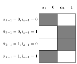
In the rank-3 site tensor , only those components satisfying the even parity condition can be nonzero. In total, there are eight possible combinations for the three indices . Within these eight elements, half are nonzero. This property is shown in Fig. 2, where the nonzero combinations are indicated by gray blocks. In numerical implementations, this allows us to save half of the memory usage.
In the following, by considering the single-orbital Anderson impurity model as an example, we shall demonstrate how to construct and evaluate the corresponding physical quantities using the GMS representation.
VII Applications to single-orbital Anderson model
The single-orbital Anderson model is a typical open quantum system problem, with its Hamiltonian given by . The impurity acts as the system that couples to the environment which we now refer to as the bath. The impurity Hamiltonian is
| (71) |
where is the onsite energy for the impurity, denotes the spin index, is the Coulomb interaction, and () are the annihilation (creation) operators of spin up and down fermion, respectively. The bath consists of free fermions and the impurity couples to the bath via the hybridization interaction
| (72) |
The chemical potential of the bath is set to zero.
VII.1 Toulouse Model (Noninteracting Case)
Now we demonstrate how to construct the GMPS of ADT by starting from a simpler situation where the Coulomb interaction . In this case, the electrons with different spin do not interact with each other and hence, we can omit the spin index in this section. The Anderson impurity model is thus reduced to an analytically solvable model, which is referred to as the Toulouse model [140] or the Fano-Anderson model [141].
VII.1.1 Construction of
To construct , we follow the standard procedure given by Eqs. (46). After splitting , the bare impurity propagator, together with the boundary G-variables, is expressed as
| (73) |
where and is its complex conjugate. The initial condition is given by
| (74) |
It can be seen that consists of exponents of time-local quadratic G-variables. Thus, the GMPS of can be constructed by sequentially applying these exponents to the vacuum state, which is represented by a GMPS with bond dimension one. Each application of the exponent can be implemented as an application of an SMPO as defined by Eq. (55).
For numerical evaluation, we need to specify an alignment of the G-variables to store the GMPS. It should be noted that the order of alignment of G-variables defined in the G-tensor Eq. (47) can significantly affect the efficiency and the final storage performance of the construction. For instance, the most natural alignment of the G-tensor for may follow the direction of the Keldysh contour such that
| (75) |
where the boundary G-variables are placed at both ends. In this case, sequentially applying the exponents in Eq. (73) can be illustrated as
| (76) |
where the violet solid curve represents the application of the exponent of quadratic terms in the form of Eq. (55). Each violet curve doubles the bond dimensions between the sites it applies to. Since the violet curves do not intersect with each other, the final G-tensor is built up with non-intersected blocks (wrapped up by a dashed box), whose inner bond dimension is two. This alignment fully reflects the time locality of the free impurity dynamics and corresponds to the direct product of their evolution operators.
Here we give another natural but inefficient alignment of G-tensors: we separate the G-variables by their conjugation and branch as
| (77) |
This alignment is natural in the sense that under G-integral, a G-tensor can be converted to an overlap of fermionic states, i.e.,
| (78) |
However, applying Eq. with such an alignment gives the following schematic figure
| (79) |
It can be observed that there are many intersections between violet curves, where each intersection will double the bond dimensions it covers. The GMPS of constructed in this way is difficult to compress, i.e., the MPS compression can almost not reduce the bond dimension. Therefore, the bond dimensions would increase dramatically with this alignment.
Although the alignment defined by Eq. (76) is optimal for , it is not friendly for . A compromise should be made for global efficiency. We have thus chosen an alignment in which G-variables at the same time step are grouped together
| (80) |
Such an alignment can be illustrated as
| (81) |
VII.1.2 Construction of
The IF consists of several exponents of quadratic G-variables, thus the most direct way to construct its GMPS is by sequentially applying the corresponding SMPOs. The MPS compression algorithm is much more effective for , but the alignment of the G-tensor would still greatly affects the bond dimensions. Here, we group G-variables at the same time step together, which gives the same alignment as (81) without the boundary G-variables.
Unlike the situation for , the G-variables in exponents are correlated to each other in a time nonlocal manner. Because of this time nonlocality, the SMPO may cover a long distance and double the bond dimensions by its coverage, and we need to apply compression algorithm after every application of an SMPO. In total, we need compression, which is inefficient. We seek a more efficient way following the spirit of TEMPO [83, 142, 114]. Instead of directly applying the SMPO, we write as a product of partial influence functionals (PIF) for which
| (82) |
Once the GMPS of the PIF is known, we can construct the IF by sequentially multiplication of PIFs. After every multiplication, we need one compression operation, giving only compressions in total.
The PIF can be constructed by directly applying the SMPOs in Eq. (82). Constructing the PIF in this way requires compressions, and constructing the IF still needs compressions. At first glance, there is no improvement. However, since the bond dimension of the PIF is usually much smaller than that of IF, a much faster construction can be achieved. This method shares a similar idea as the iterative construction described in Ref. [84].
Here is another method to construct the PIF. In a PIF , there is a common G-variable in all exponents. Thus, one can expand the PIF as
| (83) |
where only quadratic G-variable terms remain. Therefore, we need not take care the sign problem of higher-order G-variables. In this case, we may simply treat the G-variables as a raising operator acting on the vacuum state. We can thus write the PIF as an operator
| (84) |
acting on the history space. This operator can be represented as an MPO by the method discussed in Refs. [114, 89], and acting it on the vacuum state yields the desired PIF. Note that if the order of and needs to be swapped depending on the alignment of G-variables, then an extra minus sign will appear.
A third way which is more efficient and elegant to construct the PIF is to express Eq. (83) as a product of series matrices as
| (85) |
With such an expression, and by observing that G-variables in PIF can be represented as a raising operator, we can directly write the PIF as an MPO with a bond dimension two [143].
VII.1.3 Evaluation of Correlation Functions from ADT
Once the GMPS of and are constructed, we can simply merge them as the ADT . It should first be noted that the preferred alignment of the GMPS for and are not the same. The alignment (81) is preferred by but not the best alignment (76) for . In practical calculations, since constructing is much more time-consuming, the alignment as illustrated in (81) is adopted at this time.
With the ADT, any multi-time correlation function (including equal-time observables) for the impurity can be evaluated via Eq. (39), where the G-integral over a pair of G-variables is evaluated by the relation
| (86) |
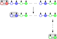
The evaluation of Eq. (39) can be achieved by iterative integration of the G-variables using the above formula. Such an iterative integration procedure is illustrated in Fig. 3.
VII.1.4 Zipup Algorithm
We now give a brief introduction of the zipup algorithm, which provides an efficient way to construct the ADT.
A direct construction of the ADT by multiplication of and would result in a large bond dimension as where and are the bond dimensions of and , respectively. The GMPS of constructed in this way is difficult to compress and thus the memory cost to store the ADT is about . The corresponding computational cost of the G-integral calculation defined by Eq. (39) is then about , which is unfriendly to numerical implementations when is large.
This is not a problem for simple cases such as the Toulouse model, where the bond dimension of the ADT is , and is only 4 with alignment given by Eq. (81). However, as we will discuss later, for the single-orbital Anderson impurity model, the bond dimension becomes . Here the term is due to two spin flavors of the bath. Even with a modest , this term yields .
Hence, it is preferable to avoid the direct construction of by multiplication of and . Instead, we can construct them on the fly when computing expectation values given by Eq. (39). Such an algorithm is referred to as the zipup algorithm in Refs. [89, 90], which boost the efficiency significantly. The basic idea of the zipup algorithm for Toulouse model is illustrated in Fig. 4, where the boundary G-variables are omitted.
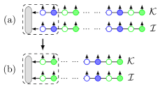
The algorithm starts with a trivial tensor , which is denoted as the vertical gray bar in Fig. 4(a). At the first step, this trivial tensor and the leftmost pair G-variables of and are multiplied together. The G-variables then are integrated out (indicated by the gray box) resulting in a new tensor [gray bar in Fig. 4(b)]. The G-integral (39) can be done via applying this procedure iteratively. The memory cost of the zipup algorithm is about since we do not need to merge and . This is clearly much less than .
Let us now check the computational cost. In one step of the zipup algorithm, the tensors in the dashed box are multiplied together. The leg of the gray bar connecting has the bond dimension , and the leg connecting has the bond dimension . To multiply them together, we can first multiply and , and this is equivalent to the multiplication of a matrix and a matrix. The corresponding computational cost is about . Then we can multiply the part, the computational cost is then about . In addition, during the zipup process, we need to swap the G-variables locally to the proper position for G-integral, which gives a cost of about . Therefore, the overall cost is about , which is significantly less than .
VII.2 Single-orbital Anderson Impurity Model
Now we proceed to the Anderson impurity model, where we need to consider the interaction term and G-variables with spin-up and spin-down flavors. The bare impurity propagator is then
| (87) |
where and
| (88) | ||||
| (89) |
with and being its complex conjugate. Once an alignment is chosen, we can apply the exponents in Eq. (87) to a vacuum GMPS sequentially to obtain the GMPS of . In practice, we align these G-variables as (the boundary G-variables are omitted here)
| (90) |
The IF for both spin flavors and are same as those of the Toulouse model, which can be obtained following the same procedure described in Sec. VII.1.2. Once the IF are known, we can use the zipup algorithm to calculate the desired quantities. The zipup algorithm is illustrated in Fig. 5.
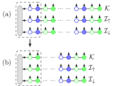
The zipup algorithm here deals with three GMPSs and . Let be the bond dimension of . It follows that the bond dimension of the ADT will be and we need to store the ADT. The computational cost of the G-integral procedure for ADT would be about . With the zipup algorithm, the memory cost would be reduced to and the computational cost would be reduced to . The zipup algorithm can be generalized to handle more GMPSs straightforwardly, as discussed in Ref. [90].
VIII Numerical examples
In this section, we review some numerical results from Refs. [89, 90, 91, 143, 144, 145, 146] which demonstrate the capability of the GTEMPO method in various applications. These include real-time dynamics for nonequilibrium situations, real-time and imaginary-time equilibration dynamics, and spectral function extraction as an impurity solver. These results are benchmarked against other methods, including continuous-time quantum Monte Carlo, the tensor-network influence functional method [84], and exact diagonalization.
VIII.1 Real-time dynamics
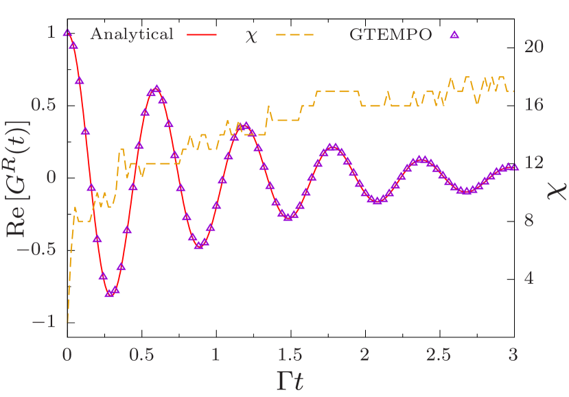
To begin with, we show the benchmarks of GTEMPO results with the analytical solution for the Toulouse model. The comparison of the retarded Green’s function between the GTEMPO results and the analytical solution are shown in Fig. 6 modified from Ref. [89]. The GTEMPO results demonstrate a good agreement with the analytical solution. In addition, the growth of the bond dimension with respect to time is also shown by the yellow dashed line. Notably, the bond dimension almost stops growing at , where denotes the system-bath coupling strength and is used as the unit scale. The bond dimension required for the Toulouse model is around 16, which is very modest.
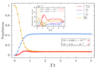
In the case of Anderson impurity model where , we show the populations of different state in the system, which are of fundamental interests in Anderson impurity model. The transient dynamics of the population calculated by GTEMPO are benchmarked against other tensor-network influence functional approach in Ref. [84], and the results are shown in Fig. 7 [89]. The system starts from the vacuum state , and after evolution it reaches the steady state where the populations of all four states remains nonzero values.
Another useful application of GTEMPO is to study the nonequilibrium dynamics of the single-orbital Anderson impurity model with multiple baths. An advantage of the path integral formalism is that we just need to deal with a single hybridization function for all baths to compute the influence functional defined in Eq. (36), i.e.,
| (91) |
where is the hybridization function for the -th bath. As such, we need to construct only a single effective IF for all baths, rather than computing the IFs for different baths separately.
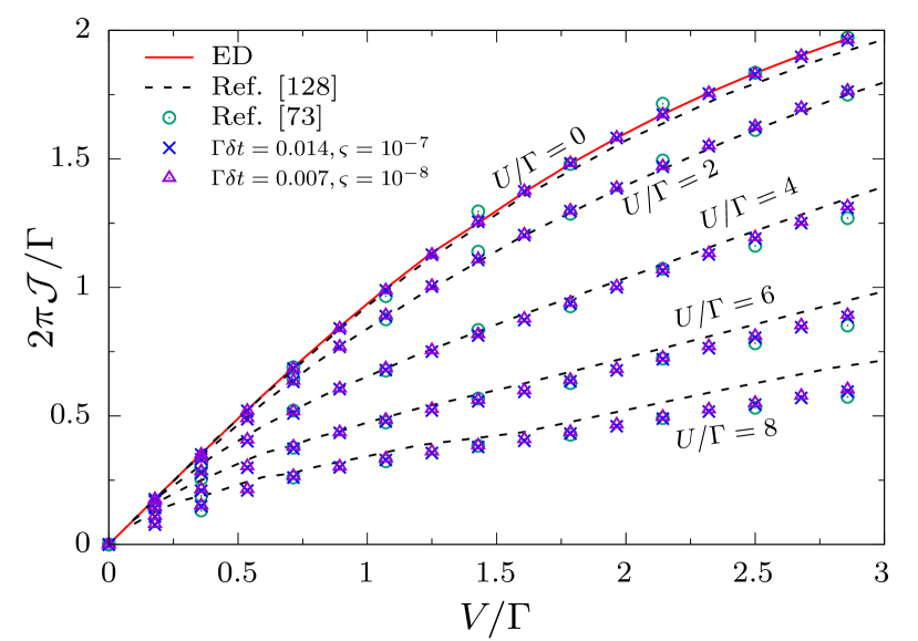
We consider the nonequilibrium single-orbital Anderson impurity model where the impurity is coupled to two baths kept at different voltages. In such a scenario, the quantity of interest is the current, which is a key indicator of transport properties. We examine the particle current with spin flowing out of the -th bath, defined as the rate of change of the particle number . It can be expressed by the system Green’s function and the hybridization function as
| (92) |
As shown in Fig. 8, the currents calculated by GTEMPO are benchmarked with the quantum Monte Carlo method [147] and the tensor-network IF method [85]. The results for all three different methods show good consistency across almost all parameter regimes. This demonstrates the capability of GTEMPO in studying the nonequilibrium dynamics.
VIII.2 Imaginary-time evolution for finite temperature equilibrium state
The path integral can also be formulated on the imaginary-time axis, where the GTEMPO method can be directly applied. On the imaginary-time axis, the system partition function is expressed by imaginary-time Grassmann trajectories.
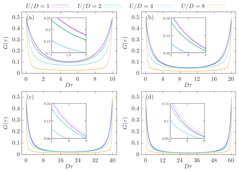
The imaginary-time calculation aims at the equilibrium properties of the model, and the Matsubara Green’s function is of particular interest. In Ref. [90], the Matsubara Green’s function for single and two-orbital Anderson impurity models are computed and benchmarked against the continuous-time Monte Carlo method [46]. Here, we just present the results for single-orbital Anderson model in Fig. 9.
An interesting phenomenon to note is that for GTEMPO, the imaginary-time calculation is more challenging than the real-time one, i.e., the bond dimension required for the imaginary-time calculation is generally much larger. This is because the imaginary path integral formalism exhibits the cyclic translational invariance, which is not suitable to be represented by open boundary MPS. An exception is the zero-temperature situation which we shall discuss later.
VIII.3 Real-time impurity solver
We can also solve the equilibrium Anderson impurity model on the real-time axis, where the GTEMPO method can be used as a real-time impurity solver [91]. The mainstream impurity solver is usually based on CTQMC, which is efficient only for imaginary-time calculations. Real-time information is extracted through analytical continuation, which is numerically ill-posed [148, 149], i.e., highly sensitive to noise. With GTEMPO, one can directly simulate the real-time dynamics of the impurity model.
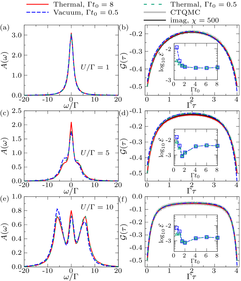
The basic procedures are summarized as follows: the model is prepared in the separate initial state Eq. (4), and then thermalized after some equilibration time by coupling to the bath. The retarded Green’s function is then calculated after this equilibration time. The spectral function can be directly extracted from the retarded Green’s function in frequency domain . This spectral function establishes a connection between the equilibrium retarded Green’s function and the Matsubara Green’s function, and can be used to calculate both the retarded and Matsubara Green’s function.
In Fig. 10, we show the spectral function obtained by GTEMPO and the corresponding Matsubara Green’s function obtained from . We benchmark these results against those from CTQMC for different . For different initial states, the GTEMPO results represented by the dashed lines are in good agreement with the CTQMC results represented by the gray shades.
IX Further developments
The GTEMPO method can also be applied to the L-shaped Kadanoff-Baym contour [150, 151], where both the imaginary-time and real-time information can be obtained simultaneously [145]. The construction procedures of and are exactly the same as those for the partial influence functional method described in this article. The only difference is that we need to replace the path integral formalism on the Keldysh contour with that on the Kadanoff-Baym contour.
On the Keldysh contour, the hybridization function (37) is time-translationally invariant. This property has not been utilized in the partial influence functional method described in this article. The implementation of time-translational invariance allows the influence functional to be constructed more efficiently [143]. In such a situation, we only need to store and manipulate GMPS sites within a single time step, and the number of GMPS multiplication needed to construct is almost independent of the evolution time.
At zero temperature (), the hybridization function differs from that at finite temperature as it always decays. Thus, the boundary condition information would eventually be lost, and open boundary MPS can again be used effectively. Moreover, at zero temperature, the hybridization also exhibits imaginary-time translational invariance. Therefore, we can also use the infinite MPS technique to construct and and directly access the ground-state information [144].
In most of the path-integral-based methods we have so far, including QuAPI, TEMPO, and GTEMPO, the steady state is obtained through finite-time evolution, which can still be a long transient dynamics. In fact, by utilizing time translational invariance and the infinite MPS technique, we can directly target the infinite time limit where the steady state is reached. Here, the steady state can be either an equilibrium or a nonequilibrium one. In such infinite time calculations, the transient dynamics information is completely lost, and only the GMPS sites within a single time step need to be stored and manipulated. At this time, the infinite GMPS is most recommended for both equilibrium and nonequilibrium steady state calculations, and more details can be found in Ref. [144].
X Conclusions
We present a general overview of the Grassmann time-evolving matrix product operator method, a numerical implementation for fermionic influence functional to study open quantum systems. As its name suggests, it shares a similar spirit with the bosonic version TEMPO [83]. We first review the formalism for both the bosonic and the fermionic path integral to give a clear picture the difficulty in Grassmann path integral evaluations. We then dive into the details of Grassmann tensors, signed matrix product operators, and the Grassmann matrix product states, which are developed to tackle the Grassmann algebra when operating these influence functional tensors. The construction of these objects is demonstrated with the single-orbital Anderson impurity model. The numerical benchmarks are also demonstrated to show real-time nonequilibrium dynamics, real-time and imaginary-time equilibration dynamics, and solving the spectral functions for impurity models. Some further developments are introduced mainly focused on the infinite GMPS, which is main focus of this article.
For future studies, we aim to incorporate the impurity solver in the DMFT calculations to study strongly-correlated many-body systems. Other potential applications include the study of strong-coupling quantum thermodynamics where a non-perturbative treatment is crucial. Moreover, we believe that the infrastructure of Grassmann tensor network can also be applied to other problems involved with Grassmann algebra. Lastly, we highlight that the open source package for GTEMPO introduced in this article will be available soon.
XI Acknowledgement
This work is supported by the NSFC Grant Nos. 12104328 and 12305049. C. G. is supported by the Open Research Fund from State Key Laboratory of High Performance Computing of China (Grant No. 202201-00).
References
- Breuer and Petruccione [2007] H.-P. Breuer and F. Petruccione, The Theory of Open Quantum Systems (Oxford University Press, 2007).
- de Vega and Alonso [2017] I. de Vega and D. Alonso, “Dynamics of non-Markovian open quantum systems,” Rev. Mod. Phys. 89, 015001 (2017).
- Weimer, Kshetrimayum, and Orús [2021] H. Weimer, A. Kshetrimayum, and R. Orús, “Simulation methods for open quantum many-body systems,” Rev. Mod. Phys. 93, 015008 (2021).
- Unruh [1995] W. G. Unruh, “Maintaining coherence in quantum computers,” Phys. Rev. A 51, 992–997 (1995).
- Palma, Suominen, and Ekert [1997] G. M. Palma, K.-a. Suominen, and A. Ekert, “Quantum computers and dissipation,” Proc. R. Soc. Lond. Ser. Math. Phys. Eng. Sci. 452, 567–584 (1997).
- Caldeira and Leggett [1983a] A. O. Caldeira and A. J. Leggett, “Path integral approach to quantum brownian motion,” Physica A 121, 587 (1983a).
- Caldeira and Leggett [1983b] A. Caldeira and A. Leggett, “Quantum tunnelling in a dissipative system,” Ann. Phys. 149, 374 (1983b).
- Datta [1995] S. Datta, Electronic Transport in Mesoscopic Systems (Cambridge University Press, Cambridge, 1995).
- Haug and Jauho [2008] H. Haug and A.-P. Jauho, Quantum Kinetics in Transport and Optics of Semiconductors (Springer-Verlag, Berlin Heidelberg, 2008).
- Ryndyk [2016] D. Ryndyk, Theory of Quantum Transport at Nanoscale, Vol. 184 (Springer International Publishing, Cham, 2016).
- Landi, Poletti, and Schaller [2022] G. T. Landi, D. Poletti, and G. Schaller, “Nonequilibrium boundary-driven quantum systems: Models, methods, and properties,” Rev. Mod. Phys. 94, 045006 (2022).
- Georges et al. [1996] A. Georges, G. Kotliar, W. Krauth, and M. J. Rozenberg, “Dynamical mean-field theory of strongly correlated fermion systems and the limit of infinite dimensions,” Rev. Mod. Phys. 68, 13 (1996).
- Popescu, Short, and Winter [2006] S. Popescu, A. J. Short, and A. Winter, “Entanglement and the foundations of statistical mechanics,” Nat. Phys. 2, 754–758 (2006).
- Goldstein et al. [2006] S. Goldstein, J. L. Lebowitz, R. Tumulka, and N. Zanghì, “Canonical Typicality,” Phys. Rev. Lett. 96, 050403 (2006).
- D’Alessio et al. [2016] L. D’Alessio, Y. Kafri, A. Polkovnikov, and M. Rigol, “From quantum chaos and eigenstate thermalization to statistical mechanics and thermodynamics,” Adv. Phys. 65, 239–362 (2016).
- Breuer et al. [2016] H.-P. Breuer, E.-M. Laine, J. Piilo, and B. Vacchini, “Colloquium: Non-Markovian dynamics in open quantum systems,” Rev. Mod. Phys. 88, 021002 (2016).
- Li, Hall, and Wiseman [2018] L. Li, M. J. W. Hall, and H. M. Wiseman, “Concepts of quantum non-Markovianity: A hierarchy,” Phys. Rep. 759, 1 (2018).
- Pollock et al. [2018] F. A. Pollock, C. Rodríguez-Rosario, T. Frauenheim, M. Paternostro, and K. Modi, “Non-Markovian quantum processes: Complete framework and efficient characterization,” Phys. Rev. A 97, 012127 (2018).
- Denisov et al. [2019] S. Denisov, T. Laptyeva, W. Tarnowski, D. Chruściński, and K. Życzkowski, “Universal Spectra of Random Lindblad Operators,” Phys. Rev. Lett. 123, 140403 (2019).
- Akemann et al. [2019] G. Akemann, M. Kieburg, A. Mielke, and T. Prosen, “Universal Signature from Integrability to Chaos in Dissipative Open Quantum Systems,” Phys. Rev. Lett. 123, 254101 (2019).
- Sá, Ribeiro, and Prosen [2020] L. Sá, P. Ribeiro, and T. Prosen, “Complex Spacing Ratios: A Signature of Dissipative Quantum Chaos,” Phys. Rev. X 10, 021019 (2020).
- Hamazaki et al. [2020] R. Hamazaki, K. Kawabata, N. Kura, and M. Ueda, “Universality classes of non-Hermitian random matrices,” Phys. Rev. Res. 2, 023286 (2020).
- Gemmer, Michel, and Mahler [2004] J. Gemmer, M. Michel, and G. Mahler, Quantum Thermodynamics: Emergence of Thermodynamic Behavior Within Composite Quantum Systems, Vol. 657 (Springer, Berlin, Heidelberg, 2004).
- Binder et al. [2018] F. Binder, L. A. Correa, C. Gogolin, J. Anders, and G. Adesso, eds., Thermodynamics in the Quantum Regime: Fundamental Aspects and New Directions, Vol. 195 (Springer International Publishing, Cham, 2018).
- Deffner and Campbell [2019] S. Deffner and S. Campbell, Quantum Thermodynamics: An Introduction to the Thermodynamics of Quantum Information (Morgan & Claypool Publishers, 2019).
- Talkner and Hänggi [2020] P. Talkner and P. Hänggi, “Colloquium: Statistical mechanics and thermodynamics at strong coupling: Quantum and classical,” Rev. Mod. Phys. 92, 041002 (2020).
- Prior et al. [2010] J. Prior, A. W. Chin, S. F. Huelga, and M. B. Plenio, “Efficient Simulation of Strong System-Environment Interactions,” Phys. Rev. Lett. 105, 050404 (2010).
- Chin et al. [2010] A. W. Chin, Á. Rivas, S. F. Huelga, and M. B. Plenio, “Exact mapping between system-reservoir quantum models and semi-infinite discrete chains using orthogonal polynomials,” J. Math. Phys. 51, 092109 (2010).
- Tamascelli et al. [2019] D. Tamascelli, A. Smirne, J. Lim, S. F. Huelga, and M. B. Plenio, “Efficient Simulation of Finite-Temperature Open Quantum Systems,” Phys. Rev. Lett. 123, 090402 (2019).
- Lacroix et al. [2024] T. Lacroix, B. Le Dé, A. Riva, A. J. Dunnett, and A. W. Chin, “MPSDynamics.jl: Tensor network simulations for finite-temperature (non-Markovian) open quantum system dynamics,” J. Chem. Phys. 161, 084116 (2024).
- de Vega and Bañuls [2015] I. de Vega and M.-C. Bañuls, “Thermofield-based chain-mapping approach for open quantum systems,” Phys. Rev. A 92, 052116 (2015).
- Guo et al. [2018] C. Guo, I. de Vega, U. Schollwöck, and D. Poletti, “Stable-unstable transition for a Bose-Hubbard chain coupled to an environment,” Phys. Rev. A 97, 053610 (2018).
- Xu et al. [2019] X. Xu, J. Thingna, C. Guo, and D. Poletti, “Many-body open quantum systems beyond Lindblad master equations,” Phys. Rev. A 99, 012106 (2019).
- Kohn and Santoro [2021] L. Kohn and G. E. Santoro, “Efficient mapping for Anderson impurity problems with matrix product states,” Phys. Rev. B 104, 014303 (2021).
- Kohn and Santoro [2022] L. Kohn and G. E. Santoro, “Quench dynamics of the Anderson impurity model at finite temperature using matrix product states: Entanglement and bath dynamics,” J. Stat. Mech. 2022, 063102 (2022).
- Tanimura and Kubo [1989] Y. Tanimura and R. Kubo, “Time Evolution of a Quantum System in Contact with a Nearly Gaussian-Markoffian Noise Bath,” J. Phys. Soc. Jpn. 58, 101–114 (1989).
- Jin, Zheng, and Yan [2008] J. Jin, X. Zheng, and Y. Yan, “Exact dynamics of dissipative electronic systems and quantum transport: Hierarchical equations of motion approach,” J. Chem. Phys. 128, 234703 (2008).
- Li et al. [2012] Z. Li, N. Tong, X. Zheng, D. Hou, J. Wei, J. Hu, and Y. Yan, “Hierarchical Liouville-Space Approach for Accurate and Universal Characterization of Quantum Impurity Systems,” Phys. Rev. Lett. 109, 266403 (2012).
- Dan et al. [2023] X. Dan, M. Xu, J. T. Stockburger, J. Ankerhold, and Q. Shi, “Efficient low-temperature simulations for fermionic reservoirs with the hierarchical equations of motion method: Application to the Anderson impurity model,” Phys. Rev. B 107, 195429 (2023).
- Huang et al. [2023] Y.-T. Huang, P.-C. Kuo, N. Lambert, M. Cirio, S. Cross, S.-L. Yang, F. Nori, and Y.-N. Chen, “An efficient Julia framework for hierarchical equations of motion in open quantum systems,” Commun Phys 6, 313 (2023).
- Lambert et al. [2023] N. Lambert, T. Raheja, S. Cross, P. Menczel, S. Ahmed, A. Pitchford, D. Burgarth, and F. Nori, “QuTiP-BoFiN: A bosonic and fermionic numerical hierarchical-equations-of-motion library with applications in light-harvesting, quantum control, and single-molecule electronics,” Phys. Rev. Res. 5, 013181 (2023).
- Zhang et al. [2024] D. Zhang, L. Ye, J. Cao, Y. Wang, R.-X. Xu, X. Zheng, and Y. Yan, “HEOM-QUICK2: A general-purpose simulator for fermionic many-body open quantum systems—An update,” WIREs Comput. Mol. Sci. 14, e1727 (2024).
- Makarov and Makri [1994] D. E. Makarov and N. Makri, “Path integrals for dissipative systems by tensor multiplication. condensed phase quantum dynamics for arbitrarily long time,” Chem. Phys. Lett. 221, 482 (1994).
- Makri [1995] N. Makri, “Numerical path integral techniques for long time dynamics of quantum dissipative systems,” J. Math. Phys. 36, 2430 (1995).
- Dattani, Pollock, and Wilkins [2012] N. S. Dattani, F. A. Pollock, and D. M. Wilkins, “Analytic influence functionals for numerical feynman integrals in most open quantum systems,” Quantum Phys. Lett. 1, 35 (2012).
- Gull et al. [2011] E. Gull, A. J. Millis, A. I. Lichtenstein, A. N. Rubtsov, M. Troyer, and P. Werner, “Continuous-time monte carlo methods for quantum impurity models,” Rev. Mod. Phys. 83, 349–404 (2011).
- Erpenbeck, Gull, and Cohen [2023] A. Erpenbeck, E. Gull, and G. Cohen, “Quantum Monte Carlo Method in the Steady State,” Phys. Rev. Lett. 130, 186301 (2023).
- Hu, Paz, and Zhang [1992] B. L. Hu, J. P. Paz, and Y. Zhang, “Quantum Brownian motion in a general environment: Exact master equation with nonlocal dissipation and colored noise,” Phys. Rev. D 45, 2843–2861 (1992).
- Zhang et al. [2012] W.-M. Zhang, P.-Y. Lo, H.-N. Xiong, M. W.-Y. Tu, and F. Nori, “General Non-Markovian Dynamics of Open Quantum Systems,” Phys. Rev. Lett. 109, 170402 (2012).
- Schwinger [1961] J. Schwinger, “Brownian Motion of a Quantum Oscillator,” J. Math. Phys. 2, 407–432 (1961).
- Wang, Wang, and Lü [2008] J.-S. Wang, J. Wang, and J. T. Lü, “Quantum thermal transport in nanostructures,” Eur. Phys. J. B 62, 381–404 (2008).
- Stefanucci and van Leeuwen [2013] G. Stefanucci and R. van Leeuwen, Nonequilibrium Many-Body Theory of Quantum Systems: A Modern Introduction (Cambridge University Press, Cambridge, 2013).
- Wang et al. [2013] J.-S. Wang, B. K. Agarwalla, H. Li, and J. Thingna, “Nonequilibrium green’s function method for quantum thermal transport,” Front. Phys. 9, 673 (2013).
- Redfield [1957] A. G. Redfield, “On the Theory of Relaxation Processes,” IBM J. Res. Dev. 1, 19–31 (1957).
- Fleming and Cummings [2011] C. H. Fleming and N. I. Cummings, “Accuracy of perturbative master equations,” Phys. Rev. E 83, 031117 (2011).
- Thingna, Wang, and Hänggi [2013] J. Thingna, J.-S. Wang, and P. Hänggi, “Reduced density matrix for nonequilibrium steady states: A modified Redfield solution approach,” Phys. Rev. E 88, 052127 (2013).
- Xu, Thingna, and Wang [2017] X. Xu, J. Thingna, and J.-S. Wang, “Finite coupling effects in double quantum dots near equilibrium,” Phys. Rev. B 95, 035428 (2017).
- Hartmann and Strunz [2020] R. Hartmann and W. T. Strunz, “Accuracy assessment of perturbative master equations: Embracing nonpositivity,” Phys. Rev. A 101, 012103 (2020).
- Nakajima [1958] S. Nakajima, “On Quantum Theory of Transport Phenomena: Steady Diffusion,” Prog. Theor. Phys. 20, 948–959 (1958).
- Zwanzig [1960] R. Zwanzig, “Ensemble Method in the Theory of Irreversibility,” J. Chem. Phys. 33, 1338–1341 (1960).
- Hughes, Christ, and Burghardt [2009a] K. H. Hughes, C. D. Christ, and I. Burghardt, “Effective-mode representation of non-Markovian dynamics: A hierarchical approximation of the spectral density. I. Application to single surface dynamics,” J. Chem. Phys. 131, 024109 (2009a).
- Hughes, Christ, and Burghardt [2009b] K. H. Hughes, C. D. Christ, and I. Burghardt, “Effective-mode representation of non-Markovian dynamics: A hierarchical approximation of the spectral density. II. Application to environment-induced nonadiabatic dynamics,” J. Chem. Phys. 131, 124108 (2009b).
- Martinazzo et al. [2011] R. Martinazzo, B. Vacchini, K. H. Hughes, and I. Burghardt, “Communication: Universal Markovian reduction of Brownian particle dynamics,” J. Chem. Phys. 134, 011101 (2011).
- Iles-Smith et al. [2016] J. Iles-Smith, A. G. Dijkstra, N. Lambert, and A. Nazir, “Energy transfer in structured and unstructured environments: Master equations beyond the Born-Markov approximations,” J. Chem. Phys. 144, 044110 (2016).
- Anto-Sztrikacs and Segal [2021] N. Anto-Sztrikacs and D. Segal, “Capturing non-Markovian dynamics with the reaction coordinate method,” Phys. Rev. A 104, 052617 (2021).
- Becker, Schnell, and Thingna [2022] T. Becker, A. Schnell, and J. Thingna, “Canonically Consistent Quantum Master Equation,” Phys. Rev. Lett. 129, 200403 (2022).
- Schaller and Brandes [2008] G. Schaller and T. Brandes, “Preservation of positivity by dynamical coarse graining,” Phys. Rev. A 78, 022106 (2008).
- Schaller, Zedler, and Brandes [2009] G. Schaller, P. Zedler, and T. Brandes, “Systematic perturbation theory for dynamical coarse-graining,” Phys. Rev. A 79, 032110 (2009).
- Garraway [1997] B. M. Garraway, “Nonperturbative decay of an atomic system in a cavity,” Phys. Rev. A 55, 2290–2303 (1997).
- Tamascelli et al. [2018] D. Tamascelli, A. Smirne, S. F. Huelga, and M. B. Plenio, “Nonperturbative Treatment of non-Markovian Dynamics of Open Quantum Systems,” Phys. Rev. Lett. 120, 030402 (2018).
- Lambert et al. [2019] N. Lambert, S. Ahmed, M. Cirio, and F. Nori, “Modelling the ultra-strongly coupled spin-boson model with unphysical modes,” Nat. Commun. 10, 3721 (2019).
- Chen, Arrigoni, and Galperin [2019] F. Chen, E. Arrigoni, and M. Galperin, “Markovian treatment of non-Markovian dynamics of open Fermionic systems,” New J. Phys. 21, 123035 (2019).
- Arrigoni, Knap, and von der Linden [2013] E. Arrigoni, M. Knap, and W. von der Linden, “Nonequilibrium Dynamical Mean-Field Theory: An Auxiliary Quantum Master Equation Approach,” Phys. Rev. Lett. 110, 086403 (2013).
- Dorda et al. [2014] A. Dorda, M. Nuss, W. von der Linden, and E. Arrigoni, “Auxiliary master equation approach to nonequilibrium correlated impurities,” Phys. Rev. B 89, 165105 (2014).
- Schwarz et al. [2016] F. Schwarz, M. Goldstein, A. Dorda, E. Arrigoni, A. Weichselbaum, and J. von Delft, “Lindblad-driven discretized leads for nonequilibrium steady-state transport in quantum impurity models: Recovering the continuum limit,” Phys. Rev. B 94, 155142 (2016).
- Gorini, Kossakowski, and Sudarshan [1976] V. Gorini, A. Kossakowski, and E. C. G. Sudarshan, “Completely positive dynamical semigroups of N-level systems,” J. Math. Phys. 17, 821–825 (1976).
- Lindblad [1976] G. Lindblad, “On the generators of quantum dynamical semigroups,” Commun. Math. Phys. 48, 119–130 (1976).
- Makarov and Makri [1995a] D. E. Makarov and N. Makri, “Stochastic resonance and nonlinear response in double-quantum-well structures,” Phys. Rev. B 52, R2257 (1995a).
- Makarov and Makri [1995b] D. E. Makarov and N. Makri, “Control of dissipative tunneling dynamics by continuous wave electromagnetic fields: Localization and large-amplitude coherent motion,” Phys. Rev. E 52, 5863 (1995b).
- Makri and Wei [1997] N. Makri and L. Wei, “Universal delocalization rate in driven dissipative two-level systems at high temperature,” Phys. Rev. E 55, 2475 (1997).
- Makri [1997] N. Makri, “Stabilization of localized states in dissipative tunneling systems interacting with monochromatic fields,” J. Chem. Phys. 106, 2286 (1997).
- Grifoni and Hänggi [1998] M. Grifoni and P. Hänggi, “Driven quantum tunneling,” Phys. Rep. 304, 229 (1998).
- Strathearn et al. [2018] A. Strathearn, P. Kirton, D. Kilda, J. Keeling, and B. W. Lovett, “Efficient non-markovian quantum dynamics using time-evolving matrix product operators,” Nat. Commun. 9, 3322 (2018).
- Ng et al. [2023] N. Ng, G. Park, A. J. Millis, G. K.-L. Chan, and D. R. Reichman, “Real-time evolution of anderson impurity models via tensor network influence functionals,” Phys. Rev. B 107, 125103 (2023).
- Thoenniss et al. [2023] J. Thoenniss, M. Sonner, A. Lerose, and D. A. Abanin, “Efficient method for quantum impurity problems out of equilibrium,” Phys. Rev. B 107, L201115 (2023).
- Thoenniss, Lerose, and Abanin [2023] J. Thoenniss, A. Lerose, and D. A. Abanin, “Nonequilibrium quantum impurity problems via matrix-product states in the temporal domain,” Phys. Rev. B 107, 195101 (2023).
- Kloss et al. [2023] B. Kloss, J. Thoenniss, M. Sonner, A. Lerose, M. T. Fishman, E. M. Stoudenmire, O. Parcollet, A. Georges, and D. A. Abanin, “Equilibrium quantum impurity problems via matrix product state encoding of the retarded action,” Phys. Rev. B 108, 205110 (2023).
- Park et al. [2024] G. Park, N. Ng, D. R. Reichman, and G. K.-L. Chan, “Tensor network influence functionals in the continuous-time limit: Connections to quantum embedding, bath discretization, and higher-order time propagation,” Phys. Rev. B 110, 045104 (2024).
- Chen, Xu, and Guo [2024a] R. Chen, X. Xu, and C. Guo, “Grassmann time-evolving matrix product operators for quantum impurity models,” Phys. Rev. B 109, 045140 (2024a).
- Chen, Xu, and Guo [2024b] R. Chen, X. Xu, and C. Guo, “Grassmann time-evolving matrix product operators for equilibrium quantum impurity problems,” New J. Phys. 26, 013019 (2024b).
- Chen, Xu, and Guo [2024c] R. Chen, X. Xu, and C. Guo, “Real-time impurity solver using grassmann time-evolving matrix product operators,” Phys. Rev. B 109, 165113 (2024c).
- Feynman and Vernon [1963] R. P. Feynman and F. L. Vernon, “The theory of a general quantum system interacting with a linear dissipative system,” Ann. Phys. 24, 118 (1963).
- Negele and Orland [1998] J. W. Negele and H. Orland, Quantum Many-Particle Systems (Westview Press, 1998).
- Keldysh [1965] L. V. Keldysh, “Diagram technique for non-equilibrium processes,” Soviet Physics JETP 20, 1018 (1965).
- Lifshitz and Pitaevskii [1981] E. M. Lifshitz and L. P. Pitaevskii, Course of Theoretical Physics Volume 10: Physical Kinetics (Elsevier, 1981).
- Kamenev and Levchenko [2009] A. Kamenev and A. Levchenko, “Keldysh technique and non-linear -model: Basic principles and applications,” Adv. Phys. 58, 197–319 (2009).
- Dong and Makri [2004a] K. Dong and N. Makri, “Optimizing terahertz emission from double quantum wells,” Chem. Phys. 296, 273 (2004a).
- Dong and Makri [2004b] K. Dong and N. Makri, “Quantum stochastic resonance in the strong-field limit,” Phys. Rev. A 70, 042101 (2004b).
- Nalbach and Thorwart [2009] P. Nalbach and M. Thorwart, “Landau-zener transitions in a dissipative environment: Numerically exact results,” Phys. Rev. Lett. 103, 220401 (2009).
- Thorwart, Reimann, and Hänggi [2000] M. Thorwart, P. Reimann, and P. Hänggi, “Iterative algorithm versus analytic solutions of the parametrically driven dissipative quantum harmonic oscillator,” Phys. Rev. E 62, 5808 (2000).
- Ilk and Makri [1994] G. Ilk and N. Makri, “Real time path integral methods for a system coupled to an anharmonic bath,” J. Chem. Phys. 101, 6708 (1994).
- Makri [1999] N. Makri, “The linear response approximation and its lowest order corrections: an influence functional approach,” J. Phys. Chem. B 103, 2823 (1999).
- Shao and Makri [2002] J. Shao and N. Makri, “Iterative path integral formulation of equilibrium correlation functions for quantum dissipative systems,” J. Chem. Phys. 116, 507–514 (2002).
- Schollwöck [2005] U. Schollwöck, “The density-matrix renormalization group,” Rev. Mod. Phys. 77, 259–315 (2005).
- Schollwöck [2011] U. Schollwöck, “The density-matrix renormalization group in the age of matrix product states,” Ann. Phys. 326, 96–192 (2011).
- Orús [2014] R. Orús, “A practical introduction to tensor networks: Matrix product states and projected entangled pair states,” Ann. Phys. 349, 117–158 (2014).
- Costa and Shrapnel [2016] F. Costa and S. Shrapnel, “Quantum causal modelling,” New J. Phys. 18, 063032 (2016).
- Pollock and Modi [2018] F. A. Pollock and K. Modi, “Tomographically reconstructed master equations for any open quantum dynamics,” Quantum 2, 76 (2018).
- Jørgensen and Pollock [2019] M. R. Jørgensen and F. A. Pollock, “Exploiting the causal tensor network structure of quantum processes to efficiently simulate non-markovian path integrals,” Phys. Rev. Lett. 123, 240602 (2019).
- Jørgensen and Pollock [2020] M. R. Jørgensen and F. A. Pollock, “Discrete memory kernel for multitime correlations in non-markovian quantum processes,” Phys. Rev. A 102, 052206 (2020).
- Chiu, Strathearn, and Keeling [2022] Y.-F. Chiu, A. Strathearn, and J. Keeling, “Numerical evaluation and robustness of the quantum mean-force gibbs state,” Phys. Rev. A 106, 012204 (2022).
- Fux et al. [2023] G. E. Fux, D. Kilda, B. W. Lovett, and J. Keeling, “Thermalization of a spin chain strongly coupled to its environment,” Phys. Rev. Res. 5, 033078 (2023).
- Gribben et al. [2021] D. Gribben, A. Strathearn, G. E. Fux, P. Kirton, and B. W. Lovett, “Using the environment to understand non-markovian open quantum systems,” Quantum 6, 847 (2021).
- Gribben et al. [2022] D. Gribben, D. M. Rouse, J. Iles-Smith, A. Strathearn, H. Maguire, P. Kirton, A. Nazir, E. M. Gauger, and B. W. Lovett, “Exact dynamics of nonadditive environments in non-markovian open quantum systems,” PRX Quantum 3, 010321 (2022).
- Otterpohl, Nalbach, and Thorwart [2022] F. Otterpohl, P. Nalbach, and M. Thorwart, “Hidden phase of the spin-boson model,” Phys. Rev. Lett. 129, 120406 (2022).
- Fux et al. [2021] G. E. Fux, E. P. Butler, P. R. Eastham, B. W. Lovett, and J. Keeling, “Efficient exploration of hamiltonian parameter space for optimal control of non-markovian open quantum systems,” Phys. Rev. Lett. 126, 200401 (2021).
- Chen and Xu [2023] R. Chen and X. Xu, “Non-markovian effects in stochastic resonance in a two level system,” Eur. Phys. J. Plus 138, 194 (2023).
- Popovic et al. [2021] M. Popovic, M. T. Mitchison, A. Strathearn, B. W. Lovett, J. Goold, and P. R. Eastham, “Quantum heat statistics with time-evolving matrix product operators,” PRX Quantum 2, 020338 (2021).
- Chen [2023] R. Chen, “Heat current in non-markovian open systems,” New J. Phys. 25, 033035 (2023).
- Ye and Chan [2021] E. Ye and G. K.-L. Chan, “Constructing tensor network influence functionals for general quantum dynamics,” J. Chem. Phys. 155, 044104 (2021).
- Bose [2022] A. Bose, “Pairwise connected tensor network representation of path integrals,” Phys. Rev. B 105, 024309 (2022).
- Cygorek et al. [2024] M. Cygorek, J. Keeling, B. W. Lovett, and E. M. Gauger, “Sublinear scaling in non-markovian open quantum systems simulations,” Phys. Rev. X 14, 011010 (2024).
- Link, Tu, and Strunz [2024] V. Link, H.-H. Tu, and W. T. Strunz, “Open quantum system dynamics from infinite tensor network contraction,” Phys. Rev. Lett. 132, 200403 (2024).
- Segal, Millis, and Reichman [2010] D. Segal, A. J. Millis, and D. R. Reichman, “Numerically exact path-integral simulation of nonequilibrium quantum transport and dissipation,” Phys. Rev. B 82, 205323 (2010).
- Segal, Millis, and Reichman [2011] D. Segal, A. J. Millis, and D. R. Reichman, “Nonequilibrium transport in quantum impurity models: Exact path integral simulations,” Phys. Chem. Chem. Phys. 13, 14378–14386 (2011).
- Simine and Segal [2013] L. Simine and D. Segal, “Path-integral simulations with fermionic and bosonic reservoirs: Transport and dissipation in molecular electronic junctions,” J. Chem. Phys. 138, 214111 (2013).
- Chen and Xu [2019] R. Chen and X. Xu, “Dissipative features of the driven spin-fermion system,” Phys. Rev. B 100, 115437 (2019).
- Chen [2020] R. Chen, “Landau-zener transitions in a fermionic dissipative environment,” Phys. Rev. B 101, 125426 (2020).
- Blankenbecler, Scalapino, and Sugar [1981] R. Blankenbecler, D. J. Scalapino, and R. L. Sugar, “Monte Carlo Calculations of Coupled Boson-Fermion Systems. I,” Phys. Rev. D 24, 2278 (1981).
- Klich [2003] I. Klich, Quantum Noise in Mesoscopic Physics, edited by Y. V. Nazarov (Springer Netherlands, 2003) pp. 397–402.
- Abanin and Levitov [2004] D. A. Abanin and L. S. Levitov, “Tunable fermi-edge resonance in an open quantum dot,” Phys. Rev. Lett. 93, 126802 (2004).
- Abanin and Levitov [2005] D. A. Abanin and L. S. Levitov, “Fermi-edge resonance and tunneling in nonequilibrium electron gas,” Phys. Rev. Lett. 94, 186803 (2005).
- Fidkowski and Kitaev [2011] L. Fidkowski and A. Kitaev, “Topological phases of fermions in one dimension,” Phys. Rev. B 83, 075103 (2011).
- Bultinck et al. [2017] N. Bultinck, D. J. Williamson, J. Haegeman, and F. Verstraete, “Fermionic matrix product states and one-dimensional topological phases,” Phys. Rev. B 95, 075108 (2017).
- Mortier et al. [2024] Q. Mortier, L. Devos, L. Burgelman, B. Vanhecke, N. Bultinck, F. Verstraete, J. Haegeman, and L. Vanderstraeten, “Fermionic tensor network methods,” arXiv:2404.14611 (2024).
- Gu [2013] Z.-C. Gu, “Efficient simulation of Grassmann tensor product states,” Phys. Rev. B 88, 115139 (2013).
- Yoshimura et al. [2018] Y. Yoshimura, Y. Kuramashi, Y. Nakamura, S. Takeda, and R. Sakai, “Calculation of fermionic Green functions with Grassmann higher-order tensor renormalization group,” Phys. Rev. D 97, 054511 (2018).
- Akiyama and Kadoh [2021] S. Akiyama and D. Kadoh, “More about the Grassmann tensor renormalization group,” J. High Energ. Phys. 2021, 188 (2021).
- Jordan and Wigner [1928] P. Jordan and E. Wigner, “Über das Paulische Äquivalenzverbot,” Z. Physik 47, 631–651 (1928).
- Leggett et al. [1987] A. J. Leggett, S. Chakravarty, A. T. Dorsey, M. P. A. Fisher, A. Garg, and W. Zwerger, “Dynamics of the dissipative two-state system,” Rev. Mod. Phys. 59, 1 (1987).
- Mahan [2000] G. D. Mahan, Many-Particle Physics (Springer; 3nd edition, 2000).
- Strathearn [2020] A. Strathearn, Modelling Non-Markovian Quantum Systems Using Tensor Networks (Springer International Publishing, Cham, Switzerland, 2020).
- Guo and Chen [2024a] C. Guo and R. Chen, “Efficient construction of the feynman-vernon influence functional as matrix product states,” SciPost Phys. Core 7, 063 (2024a).
- Guo and Chen [2024b] C. Guo and R. Chen, “Infinite Grassmann time-evolving matrix product operator method for zero-temperature equilibrium quantum impurity problems,” Phys. Rev. B 110, 165119 (2024b).
- Chen and Guo [2024] R. Chen and C. Guo, “Solving equilibrium quantum impurity problems on the L-shaped Kadanoff-Baym contour,” Phys. Rev. B 110, 165114 (2024).
- Guo and Chen [2024c] C. Guo and R. Chen, “Infinite grassmann time-evolving matrix product operator method in the steady state,” Phys. Rev. B 110, 045106 (2024c).
- Bertrand et al. [2019] C. Bertrand, S. Florens, O. Parcollet, and X. Waintal, “Reconstructing nonequilibrium regimes of quantum many-body systems from the analytical structure of perturbative expansions,” Phys. Rev. X 9, 041008 (2019).
- Wolf et al. [2015] F. A. Wolf, A. Go, I. P. McCulloch, A. J. Millis, and U. Schollwöck, “Imaginary-time matrix product state impurity solver for dynamical mean-field theory,” Phys. Rev. X 5, 041032 (2015).
- Fei, Yeh, and Gull [2021] J. Fei, C.-N. Yeh, and E. Gull, “Nevanlinna analytical continuation,” Phys. Rev. Lett. 126, 056402 (2021).
- Kadanoff and Baym [1962] L. P. Kadanoff and G. Baym, Quantum Statistical Mechnics (W. A. Benjamin, New York, 1962).
- Aoki et al. [2014] H. Aoki, N. Tsuji, M. Eckstein, M. Kollar, T. Oka, and P. Werner, “Nonequilibrium dynamical mean-field theory and its applications,” Rev. Mod. Phys. 86, 779 (2014).