Transfer Learning with Foundational Models for Time Series Forecasting using Low-Rank Adaptations

Abstract

High computational power and the availability of large datasets have supported the development of Foundational Models. They are a new emerging technique widely used in Generative Artificial Intelligence, characterized by their scalability and their use in Transfer Learning. The enormous and heterogeneous amounts of data used in their initial training phase, known as pre-training, give them a higher generalization capacity than any other specific model, constituting a solid base that can be adapted or adjusted to a wide range of tasks, increasing their applicability. This study proposes LLIAM, the Llama Lora-Integrated Autorregresive Model. Low-Rank Adaptations are used to enhance the knowledge of the model with diverse time series datasets, known as the fine-tuning phase. To illustrate the capabilities of our proposal, two sets of experiments have been carried out that obtained favorable and promising results with lower training times than other Deep Learning approaches. With this work, we also encourage the use of available resources (such as these pre-trained models) to avoid unnecessary and costly training, narrowing the gap between the goals of traditional Artificial Intelligence and those specified by the definition of Green Artificial Intelligence.

[label1] organization=Andalusian Research Institute in Data Science and Computational Intelligence, Department of Computer Science, University of Jaen,postcode=E-23071, state=Jaen, country=Spain [label2] organization=Leicester School of Pharmacy, DeMontfort University,postcode=LE1 7RH, state=Leicester, country=United Kingdom

1 Introduction

The advent of Foundation Models (FMs) has led to an explosion in several areas within the Machine Learning (ML) paradigm, and in particular Deep Learning (DL). FMs are a novel type of models that are trained on a large amount of data from different sources, which they use to develop a high generalization capacity. Several fields such as Natural Language Processing (NLP) or Computer Vision (CV) [1] have experienced a great evolution due to the good performance of these models in tasks related to the generation of new and meaningful content from training data, known as Generative AI [2]. In addition, their large generalization capacities allow them to be adapted easily and quickly to tasks from unknown domains. This is known as Transfer Learning (TL) [3].

A time-series is a type of data consisting of a set of measurements ordered over time. This implies the existence of temporal dependencies between the different moments observed. Their analysis makes it possible to extract these relationships in order to estimate its future value at any time, which is called Time-Series Forecasting (TSF). The similarity between processing a numerical and a textual series allows intuiting that using FMs dedicated to Language Modelling, such as Large Language Models (LLMs), can be adapted to TSF. Nevertheless, several proposals have argued and demonstrated that LLMs have the potential to perform diverse Time-Series Analysis tasks [4], including the capability of being adequate predictors without supplying additional time-series specific information to them [5].

Due to the great interest in FMs and the opportunities they offer in the field of TSF, we present a method that takes advantage of TL and exploits the capabilities of a LLM to perform this task. This proposal is notable for the fine-tuning of a well-known pretrained FM for language modelling called LLaMA [6] using an efficient technique known as Low-Rank Adaptation (LoRA) [7]. A modification of a prompting technique employed for feeding time-series as textual prompts inside these models is also introduced. The combination of these techniques altogether is called the Llama Lora-Integrated Autorregresive Model (LLIAM).

To demonstrate the capabilities of our proposal respecting different conventional DL methods and its base model (LLaMA) two experiments have been designed and performed, obtaining promising results in both of them. In the first one, we evaluate how LLIAM performs after fine-tuning it over several datasets and compare it to other DL approaches used on TSF. In the second one, we measure whether the previous adjustment improves the results with respect to LLaMA when making predictions on unknown data sets, which is called zero-shot forecasting.

The use of these models, which undergo intensive pre-training, can facilitate the development of new sustainable and environmentally friendly models, aligning with the objectives of Green AI [8]. This approach reduces the need for extensive training to address issues such as hyperparameter optimization or the selection of an ideal architecture. As a result, it allows progress to be made on a variety of topics while maintaining a balance between efficiency and effectiveness.

This paper is structured as follows: Section 2 describes the work related to our proposal, starting with the concept of time series, the main DL methods used for TSF and ending introducing the notion of Foundational Model (FM) and Large Languages Model (LLM). Section 3 presents our proposal, LLIAM, an adaptation of the famous LLaMA efficiently adapted to time series forecasting tasks. Section 4 presents the experimental framework, detailing the materials and methods used for the two experiments performed and how each model is evaluated. The results are also presented in this section. Finally, Section 5 concludes the article with some remarks drawn from the experiments conducted.

2 Related Work

Throughout the last years, TSF has been of interest to the scientific community. There are a wide number of methods designed to perform this task. In Section 2.1, we discuss the definition of the time series prediction problem, and in Section 2.2 how it has been approached using DL models for sequence modeling. Subsequently, the definition and importance of the Transfer Learning (TL) paradigm applied to Deep Learning (DL) methods is discussed in Section 2.3. Finally, the arrival of FMs and Transformer-based LLMs related to TL is presented in sections 2.4 and 2.5.

2.1 Time-series forecasting

A time-series is composed of a sequentially-collected set of observations. Depending on the number of variables recorded, they can be univariate or multivariate. A univariate time-series only collects one variable at a time, while multivariate gather at least two [9]. Also, if it presents a sampling frequency, it is said to be a discrete time-series. On the other hand, a time-series is considered continuous if it presents observations for every moment in time [10].

In our day-to-day life, there are numerous phenomena that exhibit different behaviors depending on the time at which they are observed. The measurement of the air temperature at a weather station, the occupancy of any type of service or the stock of specific products are examples whose activity is influenced by the presence of strong or weak time dependencies. Following the example of temperature, it is logical that at noon it is higher than in the morning or at night. Moreover, depending on the season, we can assume its variation.

The main purpose of TSF is to predict the future values of time-series, taking advantage of their temporal dependencies. In essence, this task is described as finding a function $f$ capable of generating $h$ predictions $\hat{Y}=\{\hat{y}_{t+1},\hat{y}_{t+2},...,\hat{y}_{t+h}\}$ given $n$ previous observations $S=\{x_{0},x_{1},x_{2},...,x_{n}\}$, minimizing the error between them and the real $Y=\{y_{t+1},y_{t+2},...,y_{t+h}\}$ ones. In this context, the number of time-steps to predict is called forecast horizon and the historic previous values of a series are called lags.

The pioneers working in this task were primarily statisticians whose algorithms depended on many time-series analysis techniques, expending much of their time designing them to extract and work with different features such as its trend, seasonal patterns or stationality properties.

2.2 Deep Learning and TSF

Machine Learning (ML) [11] is a subset of AI whose objective is bringing the capacity of learning from experience to computers without being explicitly programmed to do so. Inside this, another subset is found, known as DL [12]. Unlike ML methods, DL ones integrate the learning of representation into them, enabling the generation of representations with different levels of abstraction by stacking several processing or hidden layers. Artificial Neural Networks (ANNs) are the fundamental models used in DL techniques, being the artificial neuron the base element of their layers. ANNs are also considered to be universal approximators [13]. However, not all ANNs are considered Deep Neural Networks (DNN). When the number of hidden layers is greater than one, the model is not considered deep. These types of networks are known as Shallow Neural Networks (SNN) [14].

The great performance of DL in various fields [15] resulted in numerous proposals capable of modeling time-series without investing much time performing feature-engineering over them. Sequence-to-sequence (seq-to-seq) architectures are chosen for tasks in charge of generating a sequence through another sequence [16]. Encoder-decoder one is the standard used. It employs an encoder ($E$) for generating a latent representation (or context vector, $z$) of the input sequence, summarizing important information extracted from the series into a set of abstract features. This representation is then used by a decoder ($D$) module for generating the desired output. $E$ and $D$ are usually two DL architectures [17]. Nevertheless, the use of a full encoder-decoder architecture is not mandatory. The following paragraphs introduce the main models proposed for sequential data.

Recurrent Neural Networks

Recurrent Neural Networks (RNNs) are employed to detect patterns in sequential data such as text, time series or even genomes [18]. RNNs process an input sequence step-by-step, updating a hidden state at each one. This hidden state retains historical information of the sequence up to the current time step, providing an abstract and summarized representation of the entire input sequence once the last step is processed.

Following the seq-to-seq architecture, RNNs can be used as both encoders and decoders [19]. In instances where both components are employed, the encoder RNN processes the input sequence and generates a context vector that is equivalent to its hidden state. Subsequently, the output of the encoder RNN is employed as input for the decoder RNN, which generates the subsequent desired steps in an autoregressive fashion. Another common approach is to replace the decoder RNN with a unique dense layer or a multi-layer perceptron (MLP), which allows the inference of all the required steps in a single forward pass. This strategy is known as Multi-Input Multi-Output (MIMO) and is capable of generating a forecast horizon in a single step [20].

However, it is necessary to address a set of problems concerning these networks when processing long enough series. The loss of long-range dependencies, the vanishing or exploding gradient problem and their sequential nature are the principal ones. Improvements on RNNs have been proposed for mitigating the first two.

Long-Short Term Memory (LSTM) [21] introduce a new state, referred to as long term memory, and three gated mechanisms for updating both states based on the input data and generating the output as a combination of these states. In contrast, Gated Recurrent Units (GRU) [22] do not introduce a second state. Two alternate gates dictates what to forget and introduce into the hidden state, which is used for calculating the output of a cell. Both LSTM and GRU enhance the capacity of RNN for handling long-term dependencies while trying to mitigate the vanishing or exploding gradient problem.

Additional improvements to these networks try to enhance long-term dependencies. Bidirectional recurrent networks apply two LSTMs to the input sequence in both ways, forward and backward [23], and alternative LSTM cells with peephole connections [24] have been proven to enhance LSTM baseline performance when connecting the long-term memory with every gate.

Convolutional Neural Networks

Other proposals also aim to address the issue of computing input series sequentially. Convolutional Neural Networks (CNNs) [25, 26] are characterized by their good performance on image processing, but they have also been used for sequence modeling tasks. The main feature of these networks is the use of convolutions, as their name suggests. A convolution is an operator capable of extracting features sliding a filter, represented as a matrix, over the input data. When the input data are series, it is usual to rely on unidimensional convolutions (1DCNN). Nevertheless, these are not entirely suitable for sequence modeling tasks. These networks may disregard the temporal order of the data, incorporating subsequent observations when processing earlier ones.

Temporal Convolutional Networks (TCNs) [27] combine some of the best practices of modern convolutional architectures for sequence modeling, claiming to outperform RNNs in a broad collection of related tasks. A modification of the baseline convolutional operator originally used for audio generation [28] is employed, known as causal dilated convolution, inside the main component of these networks. This component is called residual block.

The causality of this operator allows the model to respect the temporal order of the data, while the dilatation technique maximizes the coverage of the receptive field for perceiving longer time dependencies without increasing the computational cost or the number of trainable parameters.

Transformers

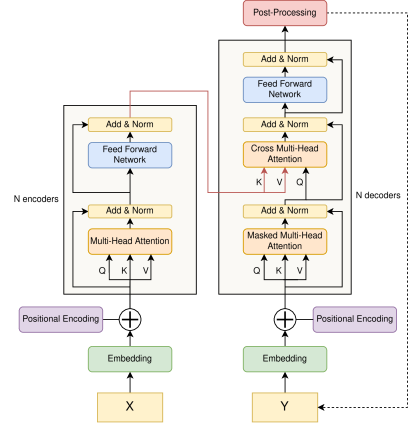
Figure 1: Transformer baseline architecture. Adapted from [17].

Transformers [17] arose as state-of-the-art architectures for sequence translation with multiple stacked encoders and decoders, capable of processing the input sequence parallelly and demonstrating superior performance compared to other classic models. As seen in figure 1, encoders and decoders are composed of Multi-Head Attention (MHA) mechanisms and Feed Forward Networks (FFN) with residual connections and layer normalization. It is important to note that while the encoder stack processes all elements of the input series in a single forward pass, the decoder follows an autoregressive fashion when predicting the output sequence.

Three attention procedures can be found in the base Transformer. The one used in the encoder is known as self-attention, and lets the model discover the different relationships between the elements of the input series. In the decoder, masked-attention utilizes a mask to prevent a position from attending future ones. Cross-attention uses the encoders stack output to find the relationships between them and the decoder input. MHA enhances the capacity of the model by simultaneously computing various attentions, referred to as “heads”, which lets it focus on different aspects of the data in each one. Note that the parallel processing of all tokens entails the need to introduce positional information into their representations to ensure that it takes into account the order of the tokens.

While MHA processes relationships between positions, FFNs are implemented at the end of all encoders and decoders to introduce non-linearity in each one separately. Between the MHA and FFN modules, residual connections and a layer normalization are applied to stabilize the learning phase of the model and improve its performance. Residual connections guarantee that the processed representations of the input tokens really represent them, and layer normalization mitigates the vanishing/exploding gradient problem for effective training.

The base architecture of Transformers has been adapted for numerous tasks, including TSF. These modifications are highly relevant today due to their strong performance across various applications. The adaptations range from simple single-component changes to entirely new architectures [29].

2.3 Transfer Learning

Using DL methods requires abundant amounts of training and test data from a specific domain to resolve tasks. However, in real-world scenarios, obtaining such data can be challenging or extremely expensive. Therefore, it is worth exploring whether knowledge from a known domain can be applied to an unknown one like humans do. This is the main purpose of transfer learning (TL) [30].

This approach focuses on improving the predictive function $f_{T}$ for a specific task $T_{T}$ within a given domain $D_{T}$ by using related information from a different task $T_{S}$ in another domain $D_{S}$. Essentially, it means borrowing knowledge from a related but different area to enhance the performance of the target task. It is crucial to understand that the source and target domains and tasks may not be the same ($D_{S}\neq D_{T}$, $T_{S}\neq T_{T}$), and each one have its own unique set of features and labels [3].

TL has been combined with numerous models from different learning paradigms to resolve specif tasks. Some examples follow. Medical images analysis tasks have benefited from this paradigm using pretrained and/or fine-tuned deep classification and segmentation models, coping with the limited amount of labeled data that can be provided in these domains [31]. Reinforcement Learning (RL) techniques have been adapted to integrate knowledge from diverse domains and their tasks, such as game playing, Natural Language Processing (NLP) and training large state-of-the-art models [32].

2.4 Foundation Models

The concept of FM was first introduced by researchers at Stanford University. FMs benefits from TL and scalability, enabled by advances in computing power and the availability of large and diverse datasets. These models serve as a robust base that can be adapted or fine-tuned for a wide range of tasks, enhancing their applicability across various domains [33]. FMs have a remarkable generalization capacity, which allows them to be proficient in several tasks without the need to be shown additional examples (zero-shot learning) or with only a few examples (few-shot learning), because they are able to learn from the context that defines their input (in-context learning).

Moreover, this input can be refined to maximize its performance with prompt-engineering techniques. It is possible to adapt its knowledge to any domain using different Parameter-Efficient Fine-Tuning (PEFT) [34, 35] techniques. This allows an efficient and fast fine-tuning of a model without the need to modify all of its weights. Although these methods arose mainly for the adaptation of LLMs, they are not limited to them or to the Transformer architecture. These can be grouped into four categories [35]: additive, which modify the model architecture to introduce new trainable components; selective, which refine only a subset of the model weights; re-parameterization, which transform the model in its fitting stage, but then integrate these transformations into its original architecture; and hybrid, which combine several methods.

Among these techniques, adapters [36] are a prominent set of methods which introduce small trainable layers between the various modules of the model. Within this category we also find prompt-tuning [37], useful in multitask language models, which seeks to adapt a human input (hard-prompt) to a more affine model (soft-prompt) by operating directly on the continuous vector space given by the model encoder. This overrides the interpretability of the original input. Similar to prompt-tuning are prefix-tuning procedures [38], which only adds a set of trainable vectors for each task faced by the model at the beginning of the input. Other frequently used techniques are Low-Rank Adaptations (LoRA) [7], which fall into the category of re-parameterization. They introduce in parallel in the modules of a model two trainable weight matrices which are combined with each other’s output, and which have a rank much smaller than the dimension of the model to be fitted. These matrices can be integrated into the original model parameters (known as the merge stage) ensuring that their inference time does not vary.

Diverse proposals have exploited the properties of FM for time-series analysis tasks, with Transformer-based architectures beign the most used [39] as they can handle sequential data effectively.

2.5 Large Language Models

LLMs are a specific type of FM trained on large amounts of textual data. Contrary to the pretrained models mentioned in Section 2.3, their superior general-purpose language understanding grants them the ability to resolve various tasks with impressive performance without requiring a fine-tuning phase. Nowadays, most of the actual architectures used by LLMs are based on the Transformer one [17].

The most famous models are currently developed and maintained by large companies. The LLaMA family is a collection of several foundational text models developed in 2013 by Meta, based on a modified Transformer decoder architecture [6]. These models are usually pretrained over a mixture of several publicly-available sources written in different languages, such as Wikipedia, GitHub or ArXiv. Improvements over this family has been made, releasing LLaMA-2 later in the same year [40] and LLaMA-3 in 2024 [41]. The differences between them focus on the increase in the quantity and quality of the data used in their pretraining phase and the use of a larger context window. Another popular family is the Generative Pretrained Transformer (GPT) one, developed and maintained by OpenAI. This was originated as an NLP multitask pretrained decoder-only Transformer model [42] and evolved into a larger and complex multi-modal one in its latest versions, such as GTP-4 [43] and GPT-4o, the last one being capable of processing audio, vision, and text in real time. Not all FMs began as LLMs. The first generation of the Gemini family from Google, for instance, started as a different decoder-only Transformer multimodal architecture. This design is suitable for various applications, from complex reasoning tasks to those requiring on-device memory constraints [44].

Time-series tasks have increasingly benefited from TL. Pretrained models, as discussed in Section 2.1, have been employed for the classification, forecasting, clustering, anomaly detection, and imputation of time-series data [45]. Transformer-based architectures are particularly significant, serving as the foundation for many models, including the well-known LLMs. These models can abstract various language domains due to the vast amounts of diverse data they are trained on. This generalization ability suggests potential applications beyond language tasks, which will be applied next, such as zero-shot TS predictors [5].

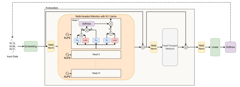
Figure 2: LLIAM arquitecture.

3 LLIAM: Llama Lora-Integrated Autorregresive Model

LLMs are pre-trained with massive amounts of data from different sources. Due to the vast volume of information that a model has to process, significant computational power and time is demanded to build such an extensive knowledge. PEFT techniques enable us to rapidly adapt these models to specific tasks, leveraging their prior knowledge. Our contribution adapts and evaluates the LLM LlaMA for TSF using the LoRA reparametrization technique based on its open-source Lit-LLaMA implementation. The resulting combination is called LLIAM: The Llama Lora-Integrated Autorregresive Model.

As mentioned in Section 2.5, the LLaMA family is a collection of several foundational text models. Multiple versions of this model with different numbers of parameters (weights) are released, ranging between 7 billion (7B) and 65 billion (65B). Our proposal employs the 7B model because it is the most lightweight one. A stacked Transformer decoder-only architecture is employed. Before entering the information into the decoder stack, the input series is transformed into a textual prompt and converted into a numerical vector using embedding. RMS Normalization is applied before processing the data in the Multi-Headed Attention module (MHA) and the Feed Forward Network (FNN) to stabilize the training of the model. MHA allows learning the relationships between the elements of the input data. An efficient implementation of it is used, with a cache that allows the recycling of previous computations to reduce the computational cost. Finally, an FFN is used to improve the features computed by MHA. The output of one decoder is used as the input of the next. Finally, the last output projected with a linear layer, used to predict the next token of the series, which will be added to the input to infer the next one.

In Figure 2 the proposed architecture of LLIAM is presented. The following paragraphs describe its main aspects.

Input Data

LLaMA can only process textual information as its input as a LLM. Time-series are prompted into the model, following a similar prompting scheme to Prompcast [46]. The numerical sequential data is transformed into textual strings following the pattern presented in Table 1. As seen, our proposal aims for a more generic pattern that does not introduce any exogenous variable or data into the prompt. In contrast with the approach proposed by Promptcast, only the number (n) and value of the input observations (series) and the desired forecast horizon (h) is provided to the model. The model is expected to only return the desired future values of the series ($t_{n+1},...,\hat{t}_{n+h}$) This will enable the use of the same template for all the datasets and evaluate the model output, relying on only its capabilities to extract the different patterns presented in the input series without providing any additional helpful information.

Promptcast	Context	From {$t_{1}$} to {$t_{n}$}, the {variable descriptor} was {series} {units} on each {frequency}
	Question	What is the {variable descriptor} going to be on the next {n+h} {frequency}?
	Answer	The {variable descriptor} will be {$t_{n+1},...,\hat{t}_{n+h}$} {units}.
LLIAM	Context	The last {n} observations of an unknown variable were {series}.
	Question	What will the next {h} observations be? Response:
	Answer	{$t_{n+1},...,\hat{t}_{n+h}$}

Table 1: Comparison between our prompting scheme and Promptcast, which it is based on. Expected answers are also provided.

Embedding

An embedding is used to transform textual tokens into vectors of continuous values in order to ensure a correct computation of the input data by the model. In LLaMA-1, each vector has a dimensionality equal to 4096 [6]. This hyperparameter is known as the dimensionality of the model ($d_{m}$), and must be consistent across all the modules of LLaMA to ensure uniformity between their inputs and outputs. Therefore, all of them will also have $d_{m}$ dimensions.

RMS Norm

Layer Normalization (LN) [47] is employed to improve and stabilize the training of the baseline Transformer after each of its modules. However, LLaMA-1 developers opted for changing what normalization technique is applied and when. Specifically, they applied Root Mean Squared Normalization (RMS Norm) [48] before processing the inputs on every module. This modification was inspired by GPT3.

Multi-Headed Attention with KV-Cache

The baseline Scaled Dot-Product Attention [17] is used in LLaMA. This mechanism is capable of learning relationships between two inputs computationally-efficiently. This procedure can be interpreted as a similarity measure between the different pair of elements that compose the input. In equation 1 is shown how this attention matrix is computed. For a given embedding of the input data $X$, three new representations are calculated, called queries ($Q$), keys ($K$) and values ($V$). Queries represent what an element of $X$ wants to attend, keys show what valuable information a token can provide and $V$ what an element really is. Each of these representations are generated by multiplying three learnable weights matrices to $X$. The similarity between the queries and keys is determined by their dot product, represented as $QK^{T}$. Higher values indicate greater similarity. A softmax function is applied to produce a probability distribution that describes how much attention each query pays to each key.

$$Attention(Q,K,V)=softmax(\frac{QK^{T}}{\sqrt{d_{k}}})V$$ (1)

Nevertheless, employing a single attention mechanism limits the range of relationship a model can notice. Consequently, many of them, known as heads, are computed with different $Q$, $K$ and $V$ representations at the same time. This is referred to as Multi-Headed Attention (MHA) and provides an enhancement of the capacity of the model, enabling the discovery of relationships at different levels. Equation 2 shows how MHA is computed. The final MHA module output is obtained by horizontally concatenating the heads and projecting them into the model’s dimensionality ($d_{model}$) using a linear layer (weights matrix $W_{O}$). In LLaMA-1 7B, the number of heads used is 32.

$$MHA(X)=Concat(head_{1},...,head_{h})W^{O}$$ (2)

$$\text{where}\quad head_{i}=Attention(XW_{i}^{Q},XW_{i}^{K},XW_{i}^{V})$$

The autoregressive nature of LLaMA leads to repeating redundant calculations that remain unchanged when adding the predicted output tokens to the input. To speed up the computation of MHA, the queries and keys of the input sentence are cached at each step. When predicting the $i^{th}$ token, two auxiliary matrices are used to retrieve these representations from the first to the $(i-1)^{th}$ token. Consequently, only the key and value for the $i^{th}$ element need to be computed instead of the full $Q$ and $V$ matrices. Also, these new values are stored in these caches, facilitating the calculation for the $(i+1)^{th}$ token.

Rotary Positional Embedding (RoPE)

Instead of using the absolute positional encoding proposed by Vaswani et al. [17], LLaMA employs a relative positional encoding method known as RoPE [49]. This technique integrates positional information into the MHA module using a 2D rotation matrix, applicable to any even-dimensional space. In essence, for an element of the input at position $m$, RoPE rotates the corresponding key and query by $m$ times a fixed angle $\theta$. When the dimensionality of the keys ($d_{K}$) and queries ($d_{V}$) are higher than two, dimensions are grouped in $d/2$ pairs and rotated following the set of different rotation angles ($\Theta$) given by equation 3.

$$\Theta=\{\theta_{i}=10000^{-2(i-1)/d},i\in[1,2,...,d/2]\}$$ (3)

Feed Forward Network (FFN)

FFNs are used at the end of each decoder to introduce non-linearity while the MHA module processes relationships between positions. The original Transformer architecture uses an FFN with a ReLU activation function. However, LLaMA-1 improves performance by using the SwiGLU activation function [50], which has been shown to outperform Transformers using ReLU on various language understanding tasks.

Low-Rank Adaptations on MHA

As introduced in Section 2.4, Low-Rank Adaptation (LoRA) [7] is a PEFT technique used for fine-tuning FMs such as LLaMA. This method can be incorporated into the model during production deployment, resulting in no additional inference latency, unlike other techniques such as adapters. LoRA was motivated by the conclusions obtained in [51], which specify that as models become larger, fewer parameters are needed to fine-tune them to achieve a certain accuracy on a specific task (a concept known as intrinsic dimension). Therefore, the change in the parameters of a model when fine-tuning may also have a low intrinsic dimension. A reparameterization such as LoRA may achieve competitive results in LLMs.

Equation LABEL:eq:lora-base describes how the LoRA technique is added into a DL module. Given a pretrained model with $W^{model}\in\mathcal{R}^{d_{m}\times k}$ weights, the change needed for fine-tuning it to a certain task is given by $\Delta W$. Based on the previous hypothesis, it must have a low intrinsic dimension. This is ensured by expressing $\Delta W$ as a low-rank decomposition of two matrices $A$ and $B$, where $A\in\mathcal{R}^{r\times k}$ and $B\in\mathcal{R}^{d_{model}\times r}$. $r$ is the hyperparameter responsible for defining the maximum desired rank of these matrices, therefore it must be $r\ll min(k,d)$. It should be noted that $W^{model}$ is not changing during the fine-tuning phase, and only $A$ and $B$ are trainable. The matrix $B$ is initialized to 0 to ensure that $\Delta W=0$ at the beginning of the training.

When processing an input matrix $X$, the output $H$ of a fine-tuned module equals to the combination of its multiplication by the original weights $W^{model}$ and by the specialized adjustment for a task given by $\Delta W$. This last component is scaled by a factor $\alpha/r$, indicating the influence of the LoRA over the output and helps to reduce the need to retune hyperparameters when $r$ is changed. $\alpha$ is set to a fixed value, thus this scale factor is not modified during fine-tuning.

$$W=W^{model}+\frac{\alpha}{r}\Delta W=W^{model}+\frac{\alpha}{r}(BA)$$ (4)

$$H=WX=W^{model}X+\frac{\alpha}{r}(BA)X$$

LoRA can be applied to almost every module of LLaMA, but we have only employed it over the queries and values projections, as illustrated in figure 2.

To conclude this section, Algorithm 1 presents the pseudo-code for the forward step of LLIAM, offering a clearer understanding of how all the modules interact. For simplicity, the initialization of RoPE and KV-Cache management has been omitted. Within the ATTENTION procedure (line 8), RoPE and LoRAs are applied to Q and V. A forward step of LLIAM produces unnormalized values (logits), which are subsequently normalized using a softmax function in the prediction step outlined in Algorithm 2. During this step, LLIAM generates predictions in an autoregressive manner. The stop criterion checks if the maximum length has been reached or if the model has outputted the end of sentence (EOS) token. After generating all the tokens, the textual output is parsed and sanitized to construct the next predicted $h$ values of the input series.

1:$n\_heads\leftarrow 32$

2:$n\_embd\leftarrow 4096$

3:$n\_layer\leftarrow 32$

4:procedure LLIAM-FORWARD($X$)

5:     $X_{coded}\leftarrow$ EMBEDDING($X$, $n\_embd$)

6:     for $decoder_{i}\quad i\in\{1,...,n\_layer\}$  do

7:         $X_{norm1}\leftarrow$ RMS-NORM($X_{coded}$)

8:         $X_{attn}\leftarrow$ ATTENTION($X_{norm1}$, $n\_heads$)

9:         $X_{res1}\leftarrow X_{attn}+X_{coded}$

10:         $X_{norm2}\leftarrow$ RMS-NORM($X_{res}$)

11:         $X_{ff}\leftarrow$ FEED-FORWARD($X_{res}$)

12:         $X_{res2}\leftarrow X_{res1}+X_{ff}$

13:         $X_{coded}\leftarrow X_{res2}$

14:     end for

15:     $Y_{norm}\leftarrow$ RMS-NORM($X_{coded}$)

16:     $Y_{logits}\leftarrow$ LINEAR($Y_{norm}$)

17:     return $Y_{logits}$

18:end procedure

Algorithm 1 LLIAM Forward Pass

1:$X\leftarrow"Prompt..."$ $\triangleright$ Textual prompt

2:procedure LLIAM-PREDICT($X$)

3:     $Y_{text}\leftarrow X$

4:     while NOT STOP-CRITERION($Y_{text}$) do

5:         $Y_{logits}\leftarrow$ LLIAM-FORWARD($Y_{text}$)

6:         $Y_{text}\leftarrow Y_{text}$ $\cup$ GET-WORD-SOFTMAX($Y_{logits}$)

7:     end while

8:     $Y_{list}\leftarrow$ PARSE-LLIAM-OUTPUT($Y_{text}$)

9:     return $Y_{list}$

10:end procedure

Algorithm 2 LLIAM Prediction Step

Since LLIAM is based on the LLaMA-1 7B model, most of its hyperparameters are identical to those detailed in [6]. Table 2 lists the main hyperparameters of LLIAM. #heads, #embd, and #decoders refer to the base model architecture, indicating the number of heads in the MHA, the embedding dimension, and the number of stacked decoders, respectively. The remaining hyperparameters relate to the LoRA architecture and training. With $r$ set to 8 and $\alpha$ set to 16, the scale factor when merging the model and LoRA outputs is 2. A light dropout is applied to the LoRA weights to prevent overfitting. The optimizer algorithm used is AdamW [52]. A micro-batch training strategy is adopted and a maximum number of training iterations is also defined. To train the LoRAs a supervised procedure is followed. The generated prompt is tokenized and transformed into a nominal representation using the SentencePieces method [53]. Then, input and target tokens are separated. The target tokens logits and the model generated logits are used to calculate a cross-entropy loss.

Hyperparameter	Value
# heads	32
# embd	4096
# decoders	32
$r$	8
$\alpha$	16
lora_dropout	0.05
learning rate	$3\cdot 10^{-4}$
batch size	128
micro bs	2
optimizer	AdamW
max iterations	75000

Table 2: LLIAM main hyperparameters

4 Experimentation framework

The main purpose of our experimentation is to demonstrate the capabilities of our LLM-based proposal, differencing two main groups of experiments. In the first group, the performance of LLIAM is compared between specific non-foundational DL methods (such as RNNs and TCNs, described in Section 2.1). Relative and absolute quality measures are computed to show the error committed by each model and their training times. This group of experiments is called “Experimental Study”.

The second group of experiments aims to show that our proposal also has a high generalization capacity. This is because it is able to tackle problems and domains never seen before, thanks to the exploitation of TL, a fundamental feature of FMs and therefore of LLMs. A series of tests have been proposed with datasets that have never been used before. The models have not been fitted with them either, so they face unknown domains and distributions of the data. This makes it possible to check whether the knowledge gain of the adapted model is significant with respect to the general knowledge of the base model, expecting in an increase of the ability to associate known concepts (in this work, series) with unknown ones. This paradigm is called Zero-Shot Learning (ZSL), so this group of experiments is called ”Zero-shot”.

This section outlines the comprehensive framework used to evaluate the proposed method. Section 4.1 details the datasets utilized and the testing procedures for LLIAM. Results from the experimental studies are presented in Section 4.2 and Zero-shot studies results are presented in Section 4.3.

4.1 Experimental seutp

The Monash University time series forecasting repository has been chosen for selecting almost every dataset used in this study. Its mission is to be the “first comprehensive repository of time series forecasts containing related time series datasets to facilitate the evaluation of global forecasting models” [54] thanks to its 30 heterogeneous sets, with different properties and coming from diverse domains. Of all the available sets, we filtered out all those where the prediction horizon was not clearly specified in the repository and were not univariate. Subsequently, we were left with only 8 main sets from this repository (Electricity, M1 Monthly, M1 Quarterly, M3 Monthly, M3 Quarterly, NN5 Daily, NN5 Weekly, San Francisco Traffic). The two Electricity Transformer Temperature (ETT) datasets [55], typically used in TSF, are also used in our study, having a total of 10 datasets employed. These datasets are described below:

• Electricity (1 Dataset): Contains the electricity consumption of 370 customers in kilowatts from 2011 to 2014. All series have the same length. Only the version whose sampling frequency is weekly has been selected.

• M1 (2 Datasets): This dataset is composed of a selection of series from one of the first competitions dedicated to its prediction, called M competitions (M, because its creator is called Makridakis). It consists of 617 monthly time series, related to economics, industry, and demography. Not all series have the same number of measurements. From it, we have selected the versions with monthly and quarterly sampling frequency.

• M3 (2 Datasets): Like the M1 dataset, it contains 1428 series from the third edition of the M competitions. They are again not of the same length and add finance-related phenomena to their domains. From it, we have selected the versions that present a monthly and quarterly sampling frequency.

• NN5 (2 Datasets): Dataset from another competition, with 111 series collecting transactions from ATMs located in Great Britain. In this case, the series have the same length. From it, we have selected the versions with a daily and weekly sampling frequency.

• San Francisco Traffic (1 Dataset): It contains 862 series collecting occupancy rates of freeways located in the San Francisco Bay Area between the years 2015 and 2016. Only the version whose sampling frequency is weekly has been selected.

• ETT (2 Datasets): Three ETT datasets were created using 2 years of data collected from two distinct counties in China. ETTh1 and ETTh2 provide data at a 1-hour granularity. Each data point includes the target value “oil temperature” which is the only feature used in our experimentation, although six additional power load features are also available.

Dataset	#Series	Frequency	H	Input size	Same Length?	Used in
electricity	321	weekly	8	65	✓	Experimental
m1	617	monthly	18	15	✗	Experimental
m1	203	quarterly	8	5	✗	Experimental
m3	1428	monthly	18	15	✗	Experimental
m3	756	quarterly	8	5	✗	Experimental
nn5	111	daily	56	9	✓	Experimental
nn5	111	weekly	8	65	✓	Experimental
San Francisco traffic	862	weekly	8	65	✓	Zero-shot
ETTh1	1	hourly	48	24	-	Zero-shot
ETTh2	1	hourly	48	24	-	Zero-shot

Table 3: Basic description of the data sets used. The columns #Series, H, Same Length and Input Size indicate the number of series in the data set, the size of the prediction horizon, the size of the input windows and whether all series have the same length. The study in which each one is used is also indicated.

A sliding window approach is used to adapt the TSF problem as a supervised learning problem. An instance consists of two windows of observations, ordered in time and without gaps. The first represents the input values to be taken by the model ($X$) and the second the expected output ($Y$), i.e., the labels. Thanks to this restructuring, we were able to transform a series into a set of $(x,y)$ pairs compatible with LLIAM. With this conversion, a textual prompt is constructed following the template described in Section 3, leaving the datasets ready to be used by the model. Table 3 shows the input window size and the prediction horizon used to construct the sliding windows for each data set, other relevant properties, and in which study each dataset is used.

model	epochs	layers	dim_h	bs	lr	%dropout
RNN-LSTM	50, 100, 200	1, 2, 4	32, 64, 128	16, 32	1e-3, 1e-2	0
RNN-GRU	50, 100, 200	1, 2, 4	32, 64, 128	16, 32	1e-3, 1e-2	0
TCN	50, 100, 200	1, 2, 4	16, 32, 64	16, 32	1e-3, 1e-2	0, 0.1, 0.25

Table 4: Hyperparameters to be used in the experimentation for each non-foundational model. dim refers to the size of the hidden state in the recurrent networks and the number of channels generated by the convolutions in the TCN. bs indicates the batch size and lr the learning rate of the optimizer.

For all the experiments, the inference hyperparameters of LLIAM will be set to default, except the temperature ($T$) with values of 10 and 20. $T$ scales the logits emited by LLIAM, which impacts directly the randomness of the model. Lower temperatures sharpens the distribution described by the output of the model, while higher ones flatten them.

The evaluation of the models is performed offline. The metrics selected are the Root Mean Square Error [56] (RMSE, equation 5), symmetric mean absolute percentage error [56] (SMAPE, equation 6).

$$RMSE=\sqrt{MSE}=\sqrt{\frac{1}{n}\sum_{t=0}^{n}(y_{t}-\hat{y_{t}})^{2}}$$ (5)

$$SMAPE=\frac{2}{n}\sum_{t=0}^{n}\frac{|y_{t}-\hat{y_{t}}|}{\max(|y_{t}|+|\hat{y_{t}}|,117\cdot 10^{-8})}$$ (6)

In the experimental study, we also observed the training time and the missing rate [46]. Given that LLMs are not inherently designed for TSF tasks, we must account for their potential to generate incorrect outputs, known as hallucinations or anomalies. In our work we classify an output as an anomaly if it fails to forecast a horizon shorter than the expected one for each dataset. If the model outputs a longer horizon, we will use only the first $h$ values and disregard the rest. The missing rate (MR) is defined in equation 7 as the difference between the number of set instances $n_{test}$ and the correctly outputted ones $n_{decoded}$ divided by the total size of the test set multiplied by 100.

$$MissingRate\%=\frac{n_{test}-n_{decoded}}{n_{test}}\cdot 100$$ (7)

4.2 Experimental study

In this study, it is tested how LLIAM is able to emit forecasts whose quality is competent in comparison with the average case presented in conventional DL models, such as RNNs and TCNs.

The methodology employed is delineated as follows. Initially, an instance of LLIAM is trained with the specified hyperparameters, as presented in Table 2. It is crucial to highlight that all seven datasets are consolidated into a unified dataset, which is employed for fine-tuning the proposed approach. In contrast, conventional DL methods, such as RNNs and TCNs, must be trained on a dataset-by-dataset basis, with all combinations of hyperparameters listed in Table 4. The metrics presented in the tables related to these algorithms are the averages of all configurations. The objective of this study is to demonstrate that LLIAM is capable of achieving performance levels that are comparable to or superior to those of these methods when a baseline hyperparameter configuration is employed. The combination of all datasets is intended to demonstrate that the comprehensive knowledge inherent to FM models, such as LLMs, enables the development of general models, reducing the necessity for time-consuming hyperparameter optimization for each dataset.

Prior to the construction of the sliding windows, a preprocessing pipeline was applied to the seven datasets. First, the heuristic methodology described in [57] is employed for the purposes of anomaly detection and mitigation. For the conventional DL methods, a min-max normalization is also applied over the full dataset to ensure the convergence of these models. After constructing the windows for each series of the dataset, the training and test sets are constructed using a leave-one-out strategy, with the last generated window of each series being used for testing. Consequently, the size of the test set is equal to the number of series in the dataset.

The results confirm our hypothesis regarding the generalization capabilities of fine-tuned LLMs for the univariate TSF task. As can be seen in Table 5, the differences between LLIAM and the other models are significant, with lower RMSE at both temperatures. For example, in the Electricity dataset, LLIAM T=10 and T=20 achieve RMSE values of 45120.043 and 42338.992 respectively, significantly outperforming the second-best model, LSTM, which achieves an RMSE of 287414.428. For the M1 monthly and quarterly data sets, LLIAM T=10 also leads with RMSE values of 2464.424 and 1913.682, outperforming the conventional DL models. The same occurs with the rest of the datasets, with our proposal achieving the lowest of the results 4 times with T=10 and three times with T=20. While the RMSE values in some datasets might seem high, they reflect the larger scale and range of the data in those specific cases. Also, it is important to note that RMSE is sensitive to anomalies. The consistently lower RMSE values of LLIAM across different datasets indicate its robustness and superior performance in the TSF task.

Unlike RMSE, SMAPE takes into account the scale of the data and determines whether a model can make predictions within the desired range. The results reported in Table 6 inform us that our propoasl. LLIAM achieves the best performance against conventional algorithms for each dataset and globally (as shown in the Avg. of Avg. column). As can be seen, compared to the best non-foundational DL model, we are able to obtain a SMAPE of 0.997 with LLIAM T=20, respecting a SMAPE of 0.232 given by the TCN D=0.1. In M1 Monthly, this performance improvement is pronounced, going from 0.436 of the TCN D=0 to 0.163 with LLIAM T=10. The M1 Quarterly results show the same tendency, obtaining a reduction of the error from 0.481 to 0.171 with LLIAM T=10. However, on the M3 and NN5 datasets the error commitment is similar between LLIAM and the other methods, achieving a small error reduction on the M3 Monthly and NN5 datasets and matching it on the M3 Quarterly with LSTM and TCN D=0 models. Overall, the performance of LLIAM T=10 and T=20 is similar, with an average SMAPE of 0.147 and 0.150 respectively, significantly outperforming all other methods.

One aspect to consider is the ability of our proposal to produce coherent and expected responses. It must be able to predict at any given time without resorting to making up hallucinations. The missing rate for each dataset and LLIAM configuration is reported in Table 7. Hallucinations were observed only on NN5 Daily for LLIAM T=10 and also on M1 Monthly for LLIAM T=20. The most frequent anomaly is due to the model stopping early, failing to reach the expected forecast horizon. Early studies showed higher missing rates, but increasing the forecast horizon by one step ($h+1$) reduced this issue. Overall, the hallucinations are not significant with respect to the results obtained.

Finally, it is necessary to consider the training time of LLIAM compared to the other models, as detailed in Table 8. Since temperature is only an inference parameter, our proposal only required one training phase. Additionally, kindly note that this only instance was trained over all the datasets with its default hyperparameters unlike LSTM, GRU and TCNs. The total time for these three methods required an exhaustive set of experiments for each configuration and dataset, resulting in a total time that exceeds the time required to train LLIAM (about 3 days compared to 18 days in the best case). Its performance suggests that fine-tuning pre-trained FMs may lead to the creation of more sustainable proposals compared to training a specific model from scratch.

	RMSE (Lower is better)
	Electricity	M1 Monthly	M1 Quarterly	M3 Monthly	M3 Quarterly	NN5 Daily	NN5 Weekly
LLIAM T=10	45120,043	2464,424	1913,682	807,877	629,930	5,918	18,342
LLIAM T=20	42338,992	2348,506	2655,757	829,951	631,046	5,906	19,085
GRU	436904,097	27405,683	29961,260	1335,165	1028,065	6,887	24,109
LSTM	287414,428	24225,724	21713,865	1265,023	964,428	6,677	22,682
TCN D=0	670686,818	34761,041	13997,682	1326,214	973,804	6,633	22,704
TCN D=0.1	663362,613	34764,894	15835,914	1347,495	1003,729	6,712	22,721
TCN D=0.25	683029,861	32666,035	17290,540	1368,059	1001,894	6,863	23,111

Table 5: RMSE metric per model and dataset. LSTM, GRU and TCN RMSE are averages for all the configurations tested, meanwhile LLIAM is the average RMSE obtained after aggregating the test instances.

	SMAPE (Lower is better)
	Electricity	M1 Monthly	M1 Quarterly	M3 Monthly	M3 Quarterly	NN5 Daily	NN5 Weekly	Avg. of Avg.
LLIAM T=10	0,099	0,163	0,171	0,150	0,102	0,232	0,114	0,147
LLIAM T=20	0,097	0,166	0,175	0,153	0,103	0,237	0,119	0,150
GRU	0,241	0,604	0,616	0,165	0,113	0,259	0,135	0,305
LSTM	0,239	0,624	0,579	0,153	0,102	0,247	0,127	0,296
TCN D=0	0,242	0,436	0,481	0,160	0,102	0,246	0,129	0,257
TCN D=0.1	0,232	0,471	0,485	0,166	0,111	0,249	0,129	0,263
TCN D=0.25	0,247	0,478	0,533	0,168	0,108	0,257	0,132	0,275

Table 6: SMAPE metric per model and dataset. LSTM, GRU and TCN SMAPE are averages for all the configurations tested, meanwhile LLIAM is the average SMAPE obtained after aggregating the test instances.

	Missing Rate % (Lower is better)
	Electricity	M1 Monthly	M1 Quarterly	M3 Monthly	M3 Quarterly	NN5 Daily	NN5 Weekly	Average
LLIAM T=10	0,000	0,000	0,000	0,000	0,000	3,604	0,000	0,5148
LLIAM T=20	0,000	0,486	0,000	0,000	0,000	6,306	0,000	0,9704

Table 7: Percentage of test instances unable to decode into the expected forecast horizon. GRU, LSTM and TCN models have been ommited because their missing rate is always 0%.

Total training time in seconds (Lower is better)
LLIAM	LSTM	GRU	TCN D=0	TCN D=0.1	TCN D=0.25
266563,780 s	1612037,888 s	1648122,031 s	1819626,881 s	1899311,350 s	1883758,756 s
3d 2h 2m 43s	18d 15h 47m 18s	19d 1h 48m 42 s	21d 1h 27m 7s	21d 23h 35m 11s	21d 19h 15m 59s

Table 8: Total training time in seconds. GRU, LSTM and TCNs training times are the sum of all the experiments made for all the configurations, meanwhile only one instance of LLIAM has been trained over all the datasets. A conversion from seconds to days (d), hours (h), minutes (m) and seconds (s) is also supplied.

4.3 Zero-shot study

In the zero-shot study we show that our adaptation of the model achieves a good degree of generalization not only for known domains, but also for unknown ones, proving that LLMs can be zero-shot forecasters as stated in [5]. The remaining 3 datasets (San Francisco traffic, ETTh1 and ETTh2) are used in this study. It is important to note that the domain of the San Francisco traffic dataset does not resemble any of the domains from the dataset used to build LLIAM. Due to the large length of the ETTh1 and ETTh2 datasets, we only used the last 10% of the generated windows to test the models. The LLaMA-1 7B base architecture is used as the baseline model, with the same temperature values used in LLIAM.

Table 9 highlights the average RMSE and SMAPE obtained for each model configuration. In ETTh1 and San Francisco traffic, the results obtained with LLIAM surpass the performance of the baseline model. However, the error between our proposal and the base model is very similar in the ETTh2 dataset. Attention may be drawn by the high average error obtained with LLAMA T=20 in the dataset ETTh1. This is produced by an anomalous behavior, where the model predicted a high value in a test window whose tendency is led by low ones. We assume that it occurred as the temperature of the model increased, since it does not occur at a value of T=10. In addition, it appears that fine-tuning with time series can also mitigate this behavior, as it did not occur when using LLIAM. Evaluating the results obtained according to the SMAPE metric, we can conclude that both metrics reach a consensus, as in the previous study. LLIAM T=10 presents a lower average SMAPE with a value of 0.171, followed by LLIAM T=20 with a similar one. This also occurs with LLAMA, obtaining an error of 0.190 with T=10 and 0.188 with T=20.

	RMSE (Lower is better)			SMAPE (Lower is better)
	ETTh1	ETTh2	Traffic	ETTh1	ETTh2	Traffic	Average SMAPE
LLIAM T=10	2,053	8,014	1,550	0,184	0,199	0,129	0,171
LLIAM T=20	2,127	8,016	1,600	0,190	0,198	0,134	0,174
LLAMA T=10	2,396	7,768	1,827	0,213	0,198	0,158	0,190
LLAMA T=20	3822528,513	7,562	1,845	0,211	0,194	0,159	0,188

Table 9: RMSE and SMAPE metric for each model and dataset on the zero-shot study. It is calculated as the average of all test instances.

5 Final discussions

This proposal introduces a novel approach to the TSF task using FMs, specifically the LLaMA model. It combines the PEFT technique LoRA with a modified PromptCast method for inputting time series data into the model. In addition, two sets of experiments have been conducted: one regarding the effectiveness and efficiency of this approach relative to others, and another to validate and compare the use of these models for TSF on unseen data sets.

The results obtained are competent and verify the outperforming of LLIAM over the other DL non-foundational methods, being capable of giving forecast with a better or equal quality than them. The intrinsic properties of FMs, highlighting it great generalization capacity by adopting TL as one of its key qualities, and the effectiveness of the fine-tuning technique used has led to the development of our proposal achieving its positive outcomes. In addition, it is noteworthy that we trained the model only once, especially considering that the training time is significantly lower compared to the total time required to train all configurations of the LSTM, GRU, and TCN models. Therefore, it is clear to say that LLIAM is more efficient.

Throughout our research, we have discussed how temperature affects the quality of the forecasts issued. As explained in Section 4.1, this hyperparameter affects the randomness of the model output. Consequently, we have only tested with low temperature values in order to respect the original non-normalized probability distribution emitted by the model. This was done to avoid unusual predictions and to encourage more deterministic ones. Light evidence has been found verifying that lower temperature values encourage better results.

The use of PEFT techniques to fine-tune pre-trained models has been widely applied to text, image, and even audio generation with good results. The sequential nature of text and audio data inspired us to try to adapt LLMs to the TSF task. As demonstrated, this initial work proved that FMs can be adequate for performing this task. However, in the case of LLMs, it is necessary to perform a tedious preliminary work to determine a number of factors related to how the data is input into them and how to adapt them. Another interesting topic to be researched is in the minimization of the missing rate, which is required to guarantee robustness with respect to the behavior of these models. Nevertheless, the opportunities offered by these types of models are extensive and constitute an interesting line of future work regarding their adaptation to different tasks as fine-tuned or zero-shot predictors.

This positive initial study marks the beginning of future work involving more extensive testing with different models of a similar nature, where they can be adapted or built specifically for TSF-related tasks. Actually, few attempts are found related to the adaptation of these FMs to these types of tasks. In addition, the exploration and creation of diverse PEFT techniques that go beyond LoRAs is also an interesting and wide-ranging aspect of the effective and efficient use and tuning of this type of models. Overall, the arrival of the FMs opens up the possibility of numerous interesting proposals.

References

- Zhou et al. [2023] C. Zhou, Q. Li, C. Li, J. Yu, Y. Liu, G. Wang, K. Zhang, C. Ji, Q. Yan, L. He, H. Peng, J. Li, J. Wu, Z. Liu, P. Xie, C. Xiong, J. Pei, P. S. Yu, L. Sun, A comprehensive survey on pretrained foundation models: A history from bert to chatgpt, 2023. URL: https://arxiv.org/abs/2302.09419. arXiv:2302.09419.
- Feuerriegel et al. [2024] S. Feuerriegel, J. Hartmann, C. Janiesch, P. Zschech, Generative ai, Business & Information Systems Engineering 66 (2024) 111–126.
- Weiss et al. [2016] K. Weiss, T. M. Khoshgoftaar, D. Wang, A survey of transfer learning, Journal of Big Data 3 (2016) 9. URL: https://doi.org/10.1186/s40537-016-0043-6. doi:10.1186/s40537-016-0043-6.
- Jin et al. [2024] M. Jin, Y. Zhang, W. Chen, K. Zhang, Y. Liang, B. Yang, J. Wang, S. Pan, Q. Wen, Position: What can large language models tell us about time series analysis, 2024. URL: https://arxiv.org/abs/2402.02713. arXiv:2402.02713.
- Gruver et al. [2023] N. Gruver, M. Finzi, S. Qiu, A. G. Wilson, Large language models are zero-shot time series forecasters, 2023. arXiv:2310.07820.
- Touvron et al. [2023] H. Touvron, T. Lavril, G. Izacard, X. Martinet, M.-A. Lachaux, T. Lacroix, B. Rozière, N. Goyal, E. Hambro, F. Azhar, A. Rodriguez, A. Joulin, E. Grave, G. Lample, Llama: Open and efficient foundation language models, 2023. arXiv:2302.13971.
- Hu et al. [2021] E. J. Hu, Y. Shen, P. Wallis, Z. Allen-Zhu, Y. Li, S. Wang, L. Wang, W. Chen, Lora: Low-rank adaptation of large language models, 2021. URL: https://arxiv.org/abs/2106.09685. arXiv:2106.09685.
- Bolón-Canedo et al. [2024] V. Bolón-Canedo, L. Morán-Fernández, B. Cancela, A. Alonso-Betanzos, A review of green artificial intelligence: Towards a more sustainable future, Neurocomputing 599 (2024) 128096. URL: https://www.sciencedirect.com/science/article/pii/S0925231224008671. doi:https://doi.org/10.1016/j.neucom.2024.128096.
- Brockwell and Davis [2016a] P. J. Brockwell, R. A. Davis, Introduction to Time Series and Forecasting, Springer Texts in Statistics, Springer International Publishing, 2016a. URL: https://doi.org/10.1007/978-3-319-29854-2. doi:10.1007/978-3-319-29854-2.
- Brockwell and Davis [2016b] P. J. Brockwell, R. A. Davis, Introduction to Time Series and Forecasting, Springer Texts in Statistics, Springer International Publishing, 2016b. URL: https://doi.org/10.1007/978-3-319-29854-2. doi:10.1007/978-3-319-29854-2.
- Sarker [2021] I. H. Sarker, Machine learning: Algorithms, real-world applications and research directions, SN Computer Science 2 (2021) 160. URL: https://doi.org/10.1007/s42979-021-00592-x. doi:10.1007/s42979-021-00592-x.
- LeCun et al. [2015] Y. LeCun, Y. Bengio, G. Hinton, Deep learning, Nature 521 (2015) 436–444. URL: https://www.nature.com/articles/nature14539. doi:10.1038/nature14539, publisher: Nature Publishing Group.
- Nielsen [2015] M. A. Nielsen, Neural networks and deep learning, 2015. URL: http://neuralnetworksanddeeplearning.com/.
- Prince [2023] S. J. Prince, Understanding Deep Learning, The MIT Press, 2023. URL: http://udlbook.com.
- Sarker [2021] I. H. Sarker, Deep learning: A comprehensive overview on techniques, taxonomy, applications and research directions, SN Computer Science 2 (2021) 420. URL: https://doi.org/10.1007/s42979-021-00815-1. doi:10.1007/s42979-021-00815-1.
- Neubig [2017] G. Neubig, Neural machine translation and sequence-to-sequence models: A tutorial, CoRR abs/1703.01619 (2017). URL: http://arxiv.org/abs/1703.01619. arXiv:1703.01619.
- Vaswani et al. [2017] A. Vaswani, et al., Attention is all you need, Proc. of NIPS 30 (2017) 5999–6009.
- Schmidt [2019] R. M. Schmidt, Recurrent Neural Networks (RNNs): A gentle Introduction and Overview, 2019. URL: http://arxiv.org/abs/1912.05911. doi:10.48550/arXiv.1912.05911, arXiv:1912.05911 [cs, stat].
- Hewamalage et al. [2021] H. Hewamalage, C. Bergmeir, K. Bandara, Recurrent neural networks for time series forecasting: Current status and future directions, International Journal of Forecasting 37 (2021) 388–427. URL: https://www.sciencedirect.com/science/article/pii/S0169207020300996. doi:https://doi.org/10.1016/j.ijforecast.2020.06.008.
- Ben Taieb et al. [2012] S. Ben Taieb, G. Bontempi, A. F. Atiya, A. Sorjamaa, A review and comparison of strategies for multi-step ahead time series forecasting based on the nn5 forecasting competition, Expert Systems with Applications 39 (2012) 7067–7083. URL: https://www.sciencedirect.com/science/article/pii/S0957417412000528. doi:https://doi.org/10.1016/j.eswa.2012.01.039.
- Hochreiter and Schmidhuber [1997] S. Hochreiter, J. Schmidhuber, Long short-term memory, Neural computation 9 (1997) 1735–80. doi:10.1162/neco.1997.9.8.1735.
- Chung et al. [2014] J. Chung, Ç. Gülçehre, K. Cho, Y. Bengio, Empirical evaluation of gated recurrent neural networks on sequence modeling, CoRR abs/1412.3555 (2014). URL: http://arxiv.org/abs/1412.3555. arXiv:1412.3555.
- Siami-Namini et al. [2019] S. Siami-Namini, N. Tavakoli, A. S. Namin, The performance of lstm and bilstm in forecasting time series, in: 2019 IEEE International Conference on Big Data (Big Data), 2019, pp. 3285–3292. doi:10.1109/BigData47090.2019.9005997.
- Gers et al. [2003] F. A. Gers, N. N. Schraudolph, J. Schmidhuber, Learning precise timing with lstm recurrent networks, J. Mach. Learn. Res. 3 (2003) 115–143. URL: https://doi.org/10.1162/153244303768966139. doi:10.1162/153244303768966139.
- LeCun et al. [1989] Y. LeCun, B. Boser, J. S. Denker, D. Henderson, R. E. Howard, W. Hubbard, L. D. Jackel, Backpropagation Applied to Handwritten Zip Code Recognition, Neural Computation 1 (1989) 541–551. URL: https://doi.org/10.1162/neco.1989.1.4.541. doi:10.1162/neco.1989.1.4.541.
- Wu [2017] J. Wu, Introduction to convolutional neural networks, National Key Lab for Novel Software Technology. Nanjing University. China 5 (2017) 495.
- Bai et al. [2018] S. Bai, J. Z. Kolter, V. Koltun, An empirical evaluation of generic convolutional and recurrent networks for sequence modeling, CoRR abs/1803.01271 (2018). URL: http://arxiv.org/abs/1803.01271. doi:doi.org/10.48550/arXiv.1803.01271. arXiv:1803.01271.
- van den Oord et al. [2016] A. van den Oord, S. Dieleman, H. Zen, K. Simonyan, O. Vinyals, A. Graves, N. Kalchbrenner, A. W. Senior, K. Kavukcuoglu, Wavenet: A generative model for raw audio, CoRR abs/1609.03499 (2016). URL: http://arxiv.org/abs/1609.03499. arXiv:1609.03499.
- Cabrera-Bermejo et al. [2023] M. I. Cabrera-Bermejo, M. J. Del Jesus, A. J. Rivera, D. Elizondo, F. Charte, M. D. Pérez-Godoy, Analysis of transformer model applications, in: Hybrid Artificial Intelligent Systems, Springer Nature Switzerland, Cham, 2023, pp. 231–243. doi:10.1007/978-3-031-40725-3_20.
- Pan and Yang [2009] S. J. Pan, Q. Yang, A survey on transfer learning, IEEE Transactions on knowledge and data engineering 22 (2009) 1345–1359.
- ATASEVER et al. [2023] S. ATASEVER, N. AZGINOGLU, D. S. TERZI, R. TERZI, A comprehensive survey of deep learning research on medical image analysis with focus on transfer learning, Clinical Imaging 94 (2023) 18–41. URL: https://www.sciencedirect.com/science/article/pii/S0899707122002856. doi:https://doi.org/10.1016/j.clinimag.2022.11.003.
- Zhu et al. [2023] Z. Zhu, K. Lin, A. K. Jain, J. Zhou, Transfer learning in deep reinforcement learning: A survey, IEEE Transactions on Pattern Analysis and Machine Intelligence 45 (2023) 13344–13362. doi:10.1109/TPAMI.2023.3292075.
- et al. [2022] R. B. et al., On the opportunities and risks of foundation models, 2022. arXiv:2108.07258.
- Xu et al. [2023] L. Xu, H. Xie, S.-Z. J. Qin, X. Tao, F. L. Wang, Parameter-efficient fine-tuning methods for pretrained language models: A critical review and assessment, 2023. URL: https://arxiv.org/abs/2312.12148. arXiv:2312.12148.
- Han et al. [2024] Z. Han, C. Gao, J. Liu, J. Zhang, S. Q. Zhang, Parameter-efficient fine-tuning for large models: A comprehensive survey, 2024. URL: https://arxiv.org/abs/2403.14608. arXiv:2403.14608.
- Houlsby et al. [2019] N. Houlsby, A. Giurgiu, S. Jastrzebski, B. Morrone, Q. de Laroussilhe, A. Gesmundo, M. Attariyan, S. Gelly, Parameter-efficient transfer learning for nlp, 2019. URL: https://arxiv.org/abs/1902.00751. arXiv:1902.00751.
- Lester et al. [2021] B. Lester, R. Al-Rfou, N. Constant, The power of scale for parameter-efficient prompt tuning, 2021. URL: https://arxiv.org/abs/2104.08691. arXiv:2104.08691.
- Li and Liang [2021] X. L. Li, P. Liang, Prefix-tuning: Optimizing continuous prompts for generation, 2021. URL: https://arxiv.org/abs/2101.00190. arXiv:2101.00190.
- Liang et al. [2024] Y. Liang, H. Wen, Y. Nie, Y. Jiang, M. Jin, D. Song, S. Pan, Q. Wen, Foundation models for time series analysis: A tutorial and survey, in: Proceedings of the 30th ACM SIGKDD Conference on Knowledge Discovery and Data Mining, 2024, pp. 6555–6565.
- Touvron et al. [2023] H. Touvron, L. Martin, K. S. et al., Llama 2: Open foundation and fine-tuned chat models, 2023. arXiv:2307.09288.
- Dubey et al. [2024] A. Dubey, A. Jauhri, et al., The llama 3 herd of models, 2024. URL: https://arxiv.org/abs/2407.21783. arXiv:2407.21783.
- Radford et al. [2018] A. Radford, K. Narasimhan, T. Salimans, I. Sutskever, Improving Language Understanding by Generative Pre-Training (2018).
- OpenAI et al. [2024] OpenAI, J. Achiam, S. Adler, S. A. et al., Gpt-4 technical report, 2024. URL: https://arxiv.org/abs/2303.08774. arXiv:2303.08774.
- Team et al. [2024] G. Team, R. Anil, S. Borgeaud, J.-B. A. et al., Gemini: A family of highly capable multimodal models, 2024. URL: https://arxiv.org/abs/2312.11805. arXiv:2312.11805.
- Ma et al. [2023] Q. Ma, Z. Liu, Z. Zheng, Z. Huang, S. Zhu, Z. Yu, J. T. Kwok, A survey on time-series pre-trained models, 2023. arXiv:2305.10716.
- Xue and Salim [2023] H. Xue, F. D. Salim, Promptcast: A new prompt-based learning paradigm for time series forecasting, 2023. URL: https://arxiv.org/abs/2210.08964. arXiv:2210.08964.
- Ba et al. [2016] J. L. Ba, J. R. Kiros, G. E. Hinton, Layer normalization, 2016. URL: https://arxiv.org/abs/1607.06450. arXiv:1607.06450.
- Zhang and Sennrich [2019] B. Zhang, R. Sennrich, Root mean square layer normalization, in: H. Wallach, H. Larochelle, A. Beygelzimer, F. d'Alché-Buc, E. Fox, R. Garnett (Eds.), Advances in Neural Information Processing Systems, volume 32, Curran Associates, Inc., 2019. URL: https://proceedings.neurips.cc/paper_files/paper/2019/file/1e8a19426224ca89e83cef47f1e7f53b-Paper.pdf.
- Su et al. [2021] J. Su, Y. Lu, S. Pan, B. Wen, Y. Liu, Roformer: Enhanced transformer with rotary position embedding, CoRR abs/2104.09864 (2021). URL: https://arxiv.org/abs/2104.09864. arXiv:2104.09864.
- Shazeer [2020] N. Shazeer, GLU variants improve transformer, CoRR abs/2002.05202 (2020). URL: https://arxiv.org/abs/2002.05202. arXiv:2002.05202.
- Aghajanyan et al. [2020] A. Aghajanyan, L. Zettlemoyer, S. Gupta, Intrinsic dimensionality explains the effectiveness of language model fine-tuning, 2020. URL: https://arxiv.org/abs/2012.13255. arXiv:2012.13255.
- Loshchilov and Hutter [2019] I. Loshchilov, F. Hutter, Decoupled weight decay regularization, 2019. URL: https://arxiv.org/abs/1711.05101. arXiv:1711.05101.
- Kudo and Richardson [2018] T. Kudo, J. Richardson, Sentencepiece: A simple and language independent subword tokenizer and detokenizer for neural text processing, 2018. URL: https://arxiv.org/abs/1808.06226. arXiv:1808.06226.
- Godahewa et al. [2021] R. Godahewa, C. Bergmeir, G. I. Webb, R. J. Hyndman, P. Montero-Manso, Monash time series forecasting archive, in: Neural Information Processing Systems Track on Datasets and Benchmarks, 2021.
- Zhou et al. [2020] H. Zhou, S. Zhang, J. Peng, S. Zhang, J. Li, H. Xiong, W. Zhang, Informer: Beyond efficient transformer for long sequence time-series forecasting, CoRR abs/2012.07436 (2020). URL: https://arxiv.org/abs/2012.07436. arXiv:2012.07436.
- Shcherbakov et al. [2013] M. V. Shcherbakov, A. Brebels, N. L. Shcherbakova, A. P. Tyukov, T. A. Janovsky, V. A. Kamaev, et al., A survey of forecast error measures, World applied sciences journal 24 (2013) 171–176.
- Martínez et al. [2019] F. Martínez, M. P. Frías, M. D. Pérez, A. J. Rivera, A methodology for applying k-nearest neighbor to time series forecasting, Artificial Intelligence Review 52 (2019) 2019–2037. URL: https://doi.org/10.1007/s10462-017-9593-z. doi:10.1007/s10462-017-9593-z.