Overcoming Domain Limitations in
Open-vocabulary Segmentation

Abstract

Open-vocabulary segmentation (OVS) has gained attention for its ability to recognize a broader range of classes. However, OVS models show significant performance drops when applied to unseen domains beyond the previous training dataset. Fine-tuning these models on new datasets can improve performance, but often leads to the catastrophic forgetting of previously learned knowledge. To address this issue, we propose a method that allows OVS models to learn information from new domains while preserving prior knowledge. Our approach begins by evaluating the input sample’s proximity to multiple domains, using precomputed multivariate normal distributions for each domain. Based on this prediction, we dynamically interpolate between the weights of the pre-trained decoder and the fine-tuned decoders. Extensive experiments demonstrate that this approach allows OVS models to adapt to new domains while maintaining performance on the previous training dataset. The source code is available at https://github.com/dongjunhwang/dwi.

1 Introduction

Open-vocabulary segmentation (OVS) has emerged as a pivotal area of research due to its potential to predict a diverse range of vocabularies without being restricted to a fixed set of predefined classes. This flexibility enables OVS models to identify new objects, rare categories, or arbitrary text-based descriptions. Recent advances in OVS (Xu et al., 2023; Yu et al., 2024) have extended its application to panoptic segmentation to recognize new classes across various segmentation tasks, such as semantic and instance segmentation.

Table 1: Segmentation performance on Cityscapes and ADE20k. Cityscapes and ADE20k are considered unseen domains in fc-clip and X-decoder, as they are previously trained on COCO. We use Panoptic Quality (PQ) as the evaluation metric.

Method	Vocab Type	Cityscapes	ADE20k
Mask2Former	Closed-set	62.1	39.7
X-Decoder	OVS	36.2	16.7
fc-clip	OVS	44.0	26.8

Despite these advancements, a limitation of OVS models is that they perform well only within the domain of the previous training dataset. As shown in Table 1, the latest OVS models (Yu et al., 2024; Zou et al., 2023a) perform worse on datasets from unseen domains compared to traditional closed-set segmentation models (Cheng et al., 2022). Although OVS models aim to recognize new classes, their ability to generalize across different unseen domains remains limited. This limitation presents challenges in real-world environments where recognizing objects in unseen domains is crucial.

Fine-tuning on the new dataset improves performance within its domain. However, after fine-tuning, OVS models face the issue of catastrophic forgetting, where they lose existing knowledge. As shown in Figure 1, this leads to a significant performance drop on the previous training dataset.

Continual learning methods offer a promising solution, as they learn new knowledge while preserving existing information. However, previous continual learning methods have limitations when applied to OVS models. We delve deeper into these challenges in Section 3.1.

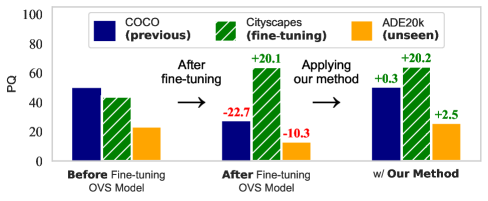
Figure 1: Performance variations after fine-tuning and applying the proposed method. The numbers above bars indicate the performance differences compared to the model before fine-tuning.

We propose a new approach that enables OVS models to generalize to new domains while preserving previous knowledge. Our method begins by fine-tuning the decoder of the OVS model on the domain of the new dataset. For this, we prepare a multivariate normal distribution (MVN) for each domain. During inference, we use these MVN distributions to infer interpolation factors that measure the proximity of the input sample to various domains. Based on this factor, we interpolate the weights of the pre-trained decoder and the fine-tuned decoders to generate new decoder weights for each input sample. This improves performance on the new dataset while preserving performance on the previous training dataset, as shown in Figure 1. Our approach does not introduce additional parameters to the OVS model and integrates seamlessly with the existing OVS architecture.

Our experimental results demonstrate that applying the proposed approach to OVS models improves performance in the new domain while maintaining performance in the previously seen domain. Specifically, when fine-tuned on Cityscapes (Cordts et al., 2016) and ADE20k (Zhou et al., 2019), the model adapts well to the new domain without losing prior knowledge. We also observe the same effect when fine-tuning the model on multiple datasets. Furthermore, the performance improves on various unseen segmentation datasets, including Mapillary Vista (Neuhold et al., 2017), LVIS (Gupta et al., 2019), and BDD100k (Yu et al., 2020).

2 Related Work

2.1 Open-vocabulary Segmentation

Open-vocabulary segmentation (OVS) addresses the limitations of traditional closed-set segmentation models, which can only recognize predefined classes. Research on closed-set segmentation models has focused on identifying objects within a fixed set of classes. However, this restriction is impractical in real-world scenarios where it is crucial to recognize new or rare classes. OVS overcomes this issue by enabling the recognition of classes not included in the training.

Existing OVS literature mainly uses models trained on large external datasets to recognize novel classes. For example, Yu et al. (2024); Zhou et al. (2022); Ding et al. (2022); Wu et al. (2023) leverage CLIP (Radford et al., 2021), a large vision-language model, with OVS models to predict classes. Recent studies also explore methods such as using a pre-trained diffusion-based model (Xu et al., 2023) or combining the Segment Anything Model (SAM) (Kirillov et al., 2023) with CLIP to recognize a variety of classes (Yuan et al., 2024; Wang et al., 2024a). OVS models trained on large-scale datasets, such as X-Decoder (Zou et al., 2023a; 2024; b), can handle OVS tasks as well as tasks like referring segmentation and image captioning. Despite these advancements, current methods remain effective only within the domain of the previous training dataset and fail to generalize to new domains. This paper addresses these unresolved issues in detail.

2.2 Fine-tuning and Catastrophic Forgetting

Fine-tuning is widely used to improve the performance of a pre-trained model on downstream tasks by adjusting the model’s parameters (Yosinski et al., 2014; Kornblith et al., 2019). Recently, instead of fine-tuning all parameters, methods have been proposed to adjust only a subset of parameters to leverage the knowledge of the pre-trained model effectively. These methods include linear probing, adapters (Houlsby et al., 2019), low-rank adaptation (Hu et al., 2021), bias tuning (Cai et al., 2020), and visual prompt tuning (VPT) (Jia et al., 2022).

Although these methods improve task-specific performance, they often overlook the problem of catastrophic forgetting. Specifically, previous OVS fine-tuning methods primarily focus on adjusting the CLIP encoder to enhance segmentation performance, but they do not address catastrophic forgetting (Xu et al., 2024; Ghiasi et al., 2022; Li et al., 2022). We are the first to highlight and analyze this issue when fine-tuning OVS models on a new domain.

Many researchers have focused on replay-based continual learning methods to address catastrophic forgetting (Chaudhry et al., 2019; Shin et al., 2017). These methods help preserve previously acquired knowledge while the model learns new tasks by using past datasets. However, storing previous datasets can raise concerns about data storage, security, and privacy. To overcome these issues, exemplar-free continual learning methods, which do not store or use past datasets, have gained attention. In this area, parameter regularization methods (Kirkpatrick et al., 2017; Ritter et al., 2018; Liu et al., 2018), function regularization methods (Li & Hoiem, 2017; Dhar et al., 2019; Iscen et al., 2020), and architecture-based approaches, including those leveraging PEFT (Wang et al., 2022a; Liang & Li, 2024; Wang et al., 2022b; Smith et al., 2023), are commonly used to solve the problem of catastrophic forgetting.

Despite various efforts to address catastrophic forgetting in continual learning, this issue remains unresolved in OVS models. In this paper, we propose a novel method to overcome this problem and expand the range of domains that OVS models can recognize.

3 Background

3.1 Motivation

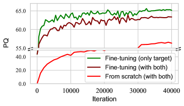
Figure 2: Comparison of performance trends of fc-clip trained on both COCO and Cityscapes versus trained only on the target dataset, Cityscapes. The evaluation is performed on the validation set of the target dataset.

When fine-tuning the OVS model on the new dataset, the model forgets previously learned knowledge. As shown in Figure 1, performance improves on the new dataset after fine-tuning, but it significantly drops on the previous training dataset. To extend the domains that the OVS model can recognize, it is necessary to address this issue of catastrophic forgetting.

One common approach to preserving existing knowledge is joint training. In this method, the OVS model is trained on both the previous training dataset and the fine-tuning dataset simultaneously, with each batch containing an equal proportion of data from both datasets. However, this approach presents three issues: 1) It requires access to all previous training datasets, which introduces challenges in data management. 2) Whether the model is trained from scratch or fine-tuned on both datasets, joint training consistently results in lower performance compared to fine-tuning on the target dataset alone (see Figure 2). 3) When there is an imbalance in the sizes of the datasets, joint training is ineffective due to the unequal representation of the datasets (Johnson & Khoshgoftaar, 2019).

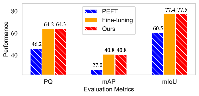
(a) Comparison of segmentation performance.

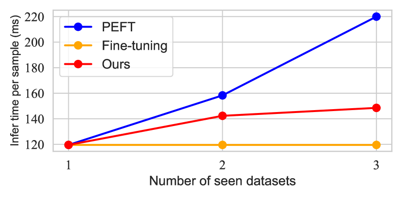
(b) Comparison of inference time.

Figure 3: (a) A comparison of segmentation performance (PQ, mAP, mIoU) between standard fine-tuning, PEFT, and our method, and (b) a comparison of average inference time per sample based on the number of datasets trained for standard fine-tuning, PEFT, and our method. All methods fine-tune fc-clip on Cityscapes, and the evaluation is performed on the Cityscapes validation set.

Another approach is exemplar-free continual learning, which resolves data management issues by eliminating the need to store previous datasets. To explore this method, we apply visual prompt tuning (VPT) (Jia et al., 2022), a PEFT approach, to the OVS model. VPT has recently shown performance improvements in the field of continual learning (Qiao et al., 2023; Wang et al., 2022c). Following the method in Kim et al. (2024), we incorporate VPT into the OVS model by adding learnable prompts to the queries and positional embeddings of the model’s decoder. However, applying this method to OVS models presents two challenges: 1) As shown in Figure 3(a), PEFT results in lower performance on the new dataset compared to fine-tuning. This likely occurs because fine-tuning optimizes a larger set of parameters, leading to greater improvements (Wortsman et al., 2022). 2) As indicated in Figure 3(b), PEFT requires additional parameters, increasing the computational resources needed for inference as the number of seen domains grows (Rypeść et al., 2024).

To address the limitations of previous techniques applied to OVS models, we propose a novel exemplar-free continual learning method. The proposed method starts by assessing the input sample’s proximity to multiple domains, using precomputed MVN distributions for each domain. Based on this, it dynamically interpolates the OVS model’s decoder weights to generate decoder weights that suit the input sample. As shown in Figure 3, the proposed method improves performance on new datasets more effectively than PEFT, while using fewer computational resources.

Problem Definition. The goal of this research is to extend the domain coverage of open-vocabulary segmentation (OVS) models through sequential fine-tuning on multiple domain-specific datasets. The OVS model is first trained on the previous training dataset $D_{pr}$, and then fine-tuned sequentially on domain-specific datasets $\{D^{1}_{ft},D^{2}_{ft},\dots\}$. In the $i$-th fine-tuning stage, the model has access only to the current dataset, $D^{i}_{ft}$. When evaluating performance, the model is tested in a setting that includes both seen datasets and unseen datasets. The unseen datasets $\{D^{1}_{\text{unseen}},D^{2}_{\text{unseen}},\dots\}$ represent datasets that the model has not been trained on before. Each dataset $D$ consists of images $X_{img}$ and class labels $X_{text}$. The main challenge is to improve performance on the new dataset $D^{i}_{ft}$ while maintaining performance on the seen datasets $\{D_{pr},D^{1}_{ft},\dots,D^{i-1}_{ft}\}$. It is also critical that the model retains or improves its ability to generalize to unseen domains.

Open-vocabulary Segmentation. We define the input image and class label as $x_{img}$ and $x_{text}$, respectively. The image encoder and text encoder are defined as $f_{img}$ and $f_{text}$, with parameters $\theta_{img}$ and $\theta_{text}$ representing the parameters of the image and text encoders. The image embedding is computed as $z_{img}=f_{img}(x_{img};\theta_{img})$, and the text embedding is computed as $z_{text}=f_{text}(x_{text};\theta_{text})$. The decoder takes these embeddings as input and predicts $N_{q}$ pairs of masks and class labels, where $N_{q}$ is the number of object queries in the decoder. Specifically, the decoder, $f_{dec}$, takes $z_{img}$ and $z_{text}$ as inputs and predicts the output $o=f_{dec}(z_{img},z_{text};\theta_{dec})$. The output $o$ consists of $N_{q}$ pairs of masks and class embeddings, $\{(m_{i},c_{i})\}_{i=1}^{N_{q}}$, where $i$ denotes the index of the pair, $m_{i}$ represents the mask, and $c_{i}$ represents the corresponding class embedding. The class associated with mask $m_{i}$ is determined by selecting the class label with the highest similarity between the predicted class embedding $c_{i}$ and the text embedding $z_{text}$. This approach allows the model to predict a wide range of classes without being limited to predefined categories.

4 Methodology

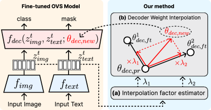
Figure 4: Inference process of our method.

This section explains the proposed method that allows OVS models to learn a new domain without losing prior knowledge. First, it describes how to generate the MVN distributions for each domain during the training phase. Then, it provides a detailed explanation of the weight interpolation process in the inference phase. An overview of the inference process is shown in Figure 4.

4.1 Training Phase

During training, we first train the OVS model using the previous training dataset. Then, we fine-tune the trained OVS model on new datasets. Following the methods of Yu et al. (2024); Zou et al. (2023a), we keep the encoder fixed during fine-tuning and only update the decoder. Notably, our approach does not modify the original training process of the OVS model, including the objective function or architecture design.

Each time we train a dataset, we calculate two sets of means and covariance matrices from the image and text embeddings. These are components of the multivariate normal (MVN) distributions. After completing the training phase, we obtain the means and covariance matrices for the previous training dataset ($i=0$) and the fine-tuning datasets ($i=1,\dots,N_{ft}$), denoted as $\{\mu^{i}_{img},\Sigma^{i}_{img},\mu^{i}_{text},\Sigma^{i}_{text}\}$.

4.2 Inference Phase

Algorithm 1 Inference Process of Our Method.

  Input: Input $(x_{img},x_{text})$, encoder $f_{img}$ & $f_{text}$, decoder $f_{dec}$, pre-trained decoder weight $\theta_{dec,pr}$, fine-tuned decoders weight $\{\theta^{1}_{dec,ft},\theta^{2}_{dec,ft},...,\theta^{N_{ft}}_{dec,ft}\}$, mean and covariance matrix $\{(\mu^{i}_{img},\Sigma^{i}_{img},\mu^{i}_{text},\Sigma^{i}_{text})\}^{N_{ft}}_{i=0}$, pdf of the MVN distribution $p$.

  Output: Mask & class pairs $\{(m_{i},c_{i})\}_{i=1}^{N_{q}}$ Step 1. Extract embedding vectors $z$. $z_{img}\leftarrow f_{img}(x_{img})$ $z_{text}\leftarrow f_{text}(x_{text})$ Step 2. Calculate the likelihood $\mathbf{l}$ for all domains. $\mathbf{l}_{img}\leftarrow\{p(z_{img}|\mu^{i}_{img},\Sigma^{i}_{img})\}^{N_{ft}}_{i=0}$ $\mathbf{l}_{text}\leftarrow\{p(z_{text}|\mu^{i}_{text},\Sigma^{i}_{text})\}^{N_{ft}}_{i=0}$ Step 3. Apply softmax and maximum to get $\bm{\lambda}$.

  $\mathbf{s}_{img}\leftarrow\text{softmax}(\mathbf{l}_{img})$

  $\mathbf{s}_{text}\leftarrow\text{softmax}(\mathbf{l}_{text})$

  $\bm{\lambda}\leftarrow\text{maximum}(\mathbf{s}_{img},\mathbf{s}_{text})$ Step 4. Interpolate the decoders weight. $\theta_{dec,new}\leftarrow\theta_{dec,pr}+\sum^{N_{ft}}_{i=1}\lambda_{i}*(\theta^{i}_{dec,ft}-\theta_{dec,pr})$ Step 5. Compute the output from the decoder. $\{(m_{i},c_{i})\}_{i=1}^{N_{q}}\leftarrow f_{dec}(z_{img},z_{text};\theta_{dec,new})$

  return  $\{(m_{i},c_{i})\}_{i=1}^{N_{q}}$

The inference process begins by calculating the interpolation factor vector $\bm{\lambda}$ (Algorithm 1, Steps 1-3). Specifically, the input image and text are passed through the encoder, producing embedding vectors for both. These embedding vectors are then fed into the probability density functions (pdf) of the image and text MVN distributions, which are defined for each domain. The image MVN distribution consists of $\mu^{i}_{img}$ and $\Sigma^{i}_{img}$, while the text MVN distribution consists of $\mu^{i}_{text}$ and $\Sigma^{i}_{text}$. This step produces a likelihood vector $l_{img}\in\mathbb{R}^{N_{ft}+1}$ for the image embedding and a likelihood vector $l_{text}\in\mathbb{R}^{N_{ft}+1}$ for the text embedding. A softmax function is then applied to these likelihood vectors, resulting in $s_{img}$ and $s_{text}$. The interpolation factor $\lambda$ for each domain is determined by selecting the maximum value from both $s_{img}$ and $s_{text}$. By considering both the image and text, this approach calculates the appropriate interpolation factor for each domain. Section 5.3 demonstrates through an ablation study that using both image and text improves performance on new domains. Figure 4a shows the interpolation factor estimator that handles this process.

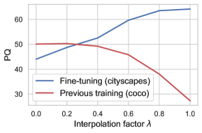
Figure 5: Performance on the validation set of Cityscapes and COCO depending on the interpolation factor $\lambda$, using fc-clip.

The calculated interpolation factor vector, $\bm{\lambda}$, is used to interpolate between the pre-trained decoder and the fine-tuned decoders (Ilharco et al., 2022) (Algorithm 1, Steps 4-5). Specifically, we multiply the difference between the weights of the domain-specific fine-tuned decoder $\theta^{i}_{dec,ft}$ and the pre-trained decoder $\theta_{dec,pr}$ by the interpolation factor $\lambda_{i}$. This determines whether the final weights are closer to the pre-trained decoder or the fine-tuned decoder. After completing this process for all the fine-tuned decoders, we sum the results to form the final interpolated decoder. The weight interpolation process is illustrated in Figure 4b.

The decoder weight interpolation process determines whether the OVS model uses the weights fitted to the previous training dataset or the fine-tuning dataset, based on the interpolation factor. As shown in Figure 5, when $\lambda_{i}=0$, the decoder uses the previously trained weights $\theta_{dec,pr}$, leading to strong performance on the previous training dataset. When $\lambda_{i}=1$, the decoder applies the fine-tuned weights $\theta^{i}_{dec,ft}$, resulting in strong performance on the fine-tuning dataset. For $\lambda_{i}$ values between 0 and 1, the decoder interpolates between the two weights, achieving moderate performance on both datasets.

Finally, the resulting decoder weights are used to predict the mask and class for the embedding of the input. The complete inference procedure with interpolation of the decoder weights, is outlined in Algorithm 1.

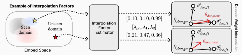
Figure 6: Illustration of $\bm{\lambda}$ generated by the interpolation factor estimator for input samples from seen and unseen domains.

Discussion. We observe that our method behaves differently depending on whether the input sample is close to the seen domain or the unseen domain. Figure 6 shows an example of the $\bm{\lambda}$ produced by the interpolation factor estimator. When the input sample is from the seen domain, it generates values close to 0 or 1. This indicates that a domain-specific model is selected for the input sample. This behavior is effective because using the model trained on the corresponding domain is optimal when the input sample is close to the seen domain.

On the other hand, for samples from the unseen domain, the interpolation factors are more evenly distributed between 0 and 1. This means that our method combines the models trained on seen domains to prevent the model from relying on a single domain. As a result, this approach improves generalization performance on input samples from the unseen domain. We demonstrate this in the Section 5.

5 Experiments

Datasets. For the panoptic segmentation task, fc-clip and X-Decoder use COCO (Lin et al., 2014) as the previous training dataset. For the fine-tuning datasets, we use Cityscapes (Cordts et al., 2016) and ADE20k (Zhou et al., 2019). For evaluation purposes only, we assess model performance on eight unseen datasets: i) LVIS (Gupta et al., 2019), ii) BDD100K (Yu et al., 2020), iii) Mapillary Vista (Neuhold et al., 2017), iv) Pascal Context (Mottaghi et al., 2014) with 59 common classes (PC-59), v) Pascal Context with all 459 classes (PC-459), vi) PASCAL VOC (Everingham et al., 2010) with 20 foreground classes (PAS-20), vii) an extension of PAS-20 with an additional background class (PAS-21), and viii) A-847, which includes all 847 classes from ADE20K (Zhou et al., 2019).

Evaluation Metrics. We evaluate all OVS models on the tasks of open-vocabulary panoptic, instance, and semantic segmentation. For evaluation, we use the Panoptic Quality (PQ) (Kirillov et al., 2019), mean Average Precision (mAP), and mean Intersection over Union (mIoU) metrics. In our experiments, PQ, mAP, and mIoU show similar performance trends. To maintain clarity, we only report PQ in the main paper and include the other metrics in the appendix.

Implementation Details. We apply our method to two OVS models: fc-clip (Yu et al., 2024) with ConvNext-L (Liu et al., 2022) backbone and X-Decoder (Zou et al., 2023a) with Focal-L (Yang et al., 2022) backbone. The fc-clip uses the CLIP (Radford et al., 2021) for both the image and text encoders, and training only decoder of the model using COCO (Lin et al., 2014). X-Decoder trains its encoder and decoder on the multiple pre-training datasets, including COCO, SBU Captions (Ordonez et al., 2011), Visual Genome (Krishna et al., 2017). Following the fc-clip and X-Decoder, we freeze the encoders and train only the decoder for both OVS models during fine-tuning. To implement the interpolation factor estimator in our method, we use the softmax temperature $T$ as $0.01$ for the softmax operation, and calculate the log-likelihood for the MVN distribution.

5.1 Compared Methods

Since there is no prior research that apply continual learning to OVS models, we apply the previous continual learning methods to the OVS models and evaluate all approaches. Following Wang et al. (2024b); Chen & Liu (2022); Parisi et al. (2019); Mundt et al. (2023), we categorize previous methods into replay-based, regularization-based (parameter, function), and architecture-based approaches. We apply a representative method from each category to OVS models and compare their performance.

Replay-based Method. Experience Replay (ER) serves as the conceptual foundation for many memory-based methods (Lopez-Paz & Ranzato, 2017; Iscen et al., 2020). In our experiments, we apply this technique to the OVS model. ER stores a subset of training samples from previous datasets and uses them during the training of a new dataset. For ER, we select 10 training samples per class from the previous training dataset. Unlike our method, ER requires access to the previous training dataset during the training of a new dataset, which makes a fair comparison difficult.

Function Regularization. We incorporate Learning without Forgetting (LwF) (Li & Hoiem, 2017), a function regularization method, into the OVS model. LwF is an exemplar-free continual learning method that uses knowledge distillation loss based on the distance between predictions of the pre-trained model and the fine-tuned model. This loss helps regularize the model to preserve its prior knowledge.

Parameter Regularization. The Elastic Weight Consolidation (EWC) (Kirkpatrick et al., 2017) method is adapted for the OVS model. EWC is a parameter regularization approach that does not rely on previous datasets. It first estimates the importance of each neuron by calculating the Fisher information matrix. This matrix assigns weights to the distance between the parameters of the pre-trained model and the fine-tuned model. This process suppresses changes to parameters that are crucial for preserving previous knowledge.

Architecture-based Method. We apply ECLIPSE (Kim et al., 2024), one of the architecture-based methods, to the OVS model. This method is designed for class-incremental learning in closed-set segmentation tasks and does not rely on the previous dataset. ECLIPSE introduces visual prompt tuning for the decoder by adding learnable prompts to the object queries and positional embedding. For our task, we add 250 prompts for each new domain to ensure sufficient learning capacity. We use only the prompt tuning component of ECLIPSE in the OVS model and do not include the classifier or logit manipulation components.

5.2 Comparison with Other Methods

Table 2: Performance comparison between standard fine-tuning, previous continual learning methods, and our method. All methods fine-tune the models using (a) Cityscapes or (b) ADE20K datasets. PQ is used.

Method	COCO (previous)	Cityscapes (fine-tuning)	ADE20K (unseen)
fc-clip	50.1	44.0	23.5
Fine-tuning	-22.7	+20.1	-10.3
+ ER	-1.6	+19.0	+0.3
+ LwF	-10.7	+12.2	-0.8
+ EWC	-25.9	+19.3	-9.8
+ ECLIPSE	-6.0	+2.2	+0.9
+ Ours	+0.3	+20.2	+2.5
X-Decoder	56.7	36.3	16.7
+ Fine-tuning	-50.4	+26.6	-12.9
+ Ours	-0.4	+26.6	+0.1

(a) Cityscapes

Method	COCO (previous)	ADE20K (fine-tuning)	Cityscapes (unseen)
fc-clip	50.1	23.5	44.0
+ Fine-tuning	-7.7	+24.1	-3.0
+ ER	+0.4	+21.5	-3.5
+ LwF	-3.8	+13.7	-1.0
+ EWC	-11.1	+20.7	-2.6
+ ECLIPSE	-0.5	+0.2	-5.9
+ Ours	+1.7	+23.8	-0.3
X-Decoder	56.7	16.7	36.3
+ Fine-tuning	-37.3	+28.2	-3.7
+ Ours	-1.5	+29.2	+1.4

(b) ADE20K

In each experiment, we evaluate the model on the previous training dataset (COCO), the fine-tuning dataset, and the unseen dataset. When the model is fine-tuned on Cityscapes, we treat ADE20K as the unseen dataset for evaluation, and vice versa.

Results of fine-tuning with Cityscapes. We present the evaluation results in Table 2 after fine-tuning the model on Cityscapes. Our method improves performance on the fine-tuning dataset while maintaining the performance on the previous training dataset, regardless of whether it is applied to fc-clip or X-Decoder. Specifically, compared to fine-tuning, our method preserves performance on the previous training dataset more effectively (e.g., Fine-tuning: $-22.7$, Ours: $+0.3$ for fc-clip / Fine-tuning: $-50.4$, Ours: $-0.4$ for X-Decoder), while achieving the same improvements on the fine-tuning dataset. Furthermore, we observe that other continual learning methods consistently result in performance degradation on the previous training dataset (e.g., ER: $-1.6$, LwF: $-10.7$, EWC: $-25.9$, ECLIPSE: $-6.0$). In contrast, our method preserves performance on the previous training dataset (e.g., Ours: $+0.3$) and achieves better results on both the fine-tuning and unseen datasets.

Results of fine-tuning with ADE20K. We present the evaluation results of our method and previous methods when fine-tuning on ADE20K in Table 2. Since ADE20K shares a similar domain with COCO, previous methods maintain performance on the previous training dataset compared to fine-tuning on Cityscapes. However, they still show a consistent performance drop on unseen datasets. In contrast, our method improves performance on the unseen dataset while also enhancing results on the previous training dataset and achieving a significant boost on the fine-tuning dataset (e.g., fc-clip with ours: previous training $+1.7$, fine-tuning $+23.8$, unseen $-0.3$). The improvement on the previous training dataset indicates that our method not only preserves prior knowledge but also enhances performance in the previously trained domain by leveraging new knowledge. Additionally, X-Decoder loses performance on the previous training dataset with standard fine-tuning, but with our method, this performance is effectively preserved (e.g., X-Decoder with ours: $-1.5$ on the previous training dataset).

Table 3: Performance of standard fine-tuning and our proposed method. The best performance for each dataset is underlined. City→ADE refers to the model fine-tuned on the Cityscapes dataset first, followed by ADE20K. The reverse applies to ADE→City. PQ is used.

Method	The order of fine-tuning	COCO (previous)	ADE20K (fine-tuning 1)	Cityscapes (fine-tuning 2)
fc-clip	-	50.1	23.5	44.0
+ Fine-tuning	ADE → City	20.8	15.4	65.2
+ Fine-tuning	City → ADE	39.3	48.3	46.0
+ Ours	City, ADE	51.6	47.0	64.3

Results of fine-tuning with multiple datasets. As shown in Table 3, we compare the standard fine-tuning method with our approach in the sequential training scenario on ADE20K and Cityscapes. Fine-tuning results in a significant performance drop on previous training datasets (e.g., ADE→City: $-29.3$, City→ADE: $-10.8$ on COCO), maintaining strong performance only on the most recent training dataset. In contrast, our method improves performance on the previous training dataset (e.g., $+1.5$ on COCO) and enhances results across all fine-tuning datasets.

Table 4: Performance comparison between sequential training and our method on 8 unseen datasets. PQ is used.

Method	The order of fine-tuning	LVIS (mAP)	BDD100K (PQ)	Mapillary (mIoU)	PC-59 (mIoU)	PC-459 (mIoU)	PAS-20 (mIoU)	PAS-21 (mIoU)	A-847 (mIoU)
fc-clip	-	20.5	19.0	26.0	53.0	16.9	93.1	80.2	13.8
+ Fine-tuning	Cityscapes → ADE20k	21.7	19.7	27.8	52.1	17.2	92.3	76.7	16.0
+ Fine-tuning	ADE20k → Cityscapes	10.4	21.3	24.2	45.9	13.5	87.4	70.7	11.5
+ Ours	Cityscapes, ADE20k	23.1	22.6	29.1	54.9	17.9	93.6	80.7	16.3

As shown in Table 4, we compare the fine-tuning technique with our method on unseen datasets. Fine-tuning fails to consistently improve performance on these datasets, and in some cases, it even results in performance drops (e.g., City→ADE: $-3.3$ on PAS-21, ADE→City: $-11.1$ on LVIS). In contrast, our method achieves consistent performance improvements across all unseen datasets.

5.3 Ablation Study

Table 5: Performance comparison between the argmax and softmax operations in the interpolation factor estimator. We use fc-clip with our method and fine-tune it on both Cityscapes and ADE20K. PQ is used.

Decision Rule	Fine-tuning Dataset	LVIS (mAP)	BDD100K (PQ)	Mapillary (mIoU)	PC-59 (mIoU)	PC-459 (mIoU)	PAS-20 (mIoU)	PAS-21 (mIoU)	A-847 (mIoU)
Argmax	Cityscapes, ADE20k	21.3	18.3	26.9	53.1	17.0	93.2	80.2	16.3
Softmax	Cityscapes, ADE20k	23.1	22.6	29.1	54.9	17.9	93.6	80.7	16.3

Replacing Softmax with Argmax. In this study, we use the softmax function to calculate interpolation factors for each domain. Considering that argmax is a hard version of softmax, we compare the segmentation performance on unseen datasets when using argmax and softmax operations. Table 5 presents the evaluation results. We observe that softmax consistently outperforms argmax across all unseen domains (e.g., on LVIS, argmax: $21.3$, softmax: $23.1$). In the PAS-20, PAS-21, and A-847, there is little difference in performance between softmax and argmax. This is because the interpolation factor from softmax tends to be close to 0 or 1 when the input sample is close to the seen domain, making softmax behave similarly to argmax. As shown in Figure 7, for A-847, the interpolation factors are close to 0 or 1 because it shares a domain similar to ADE20K, a training dataset. In contrast, the interpolation factors for BDD100K are evenly distributed between 0 and 1. This occurs because BDD100K is closer to an unseen domain. In this case, our method improves generalization performance by combining models trained on multiple domains. These results indicate that considering multiple domains simultaneously via softmax leads to better performance than selecting a single domain through argmax, supporting the effectiveness of our design choice.

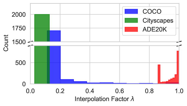
(a) A-847

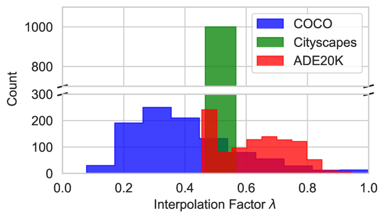
(b) BDD100K

Figure 7: The histogram of interpolation factors when inferring all samples from the validation sets of (a) A-847 and (b) BDD100K. We fine-tune fc-clip on Cityscapes and ADE20K and use PQ as the evaluation metric.

Table 6: Comparison between using both image and text or using only one type of information. Fine-tuned fc-clip on Cityscapes. PQ is used.

Distribution	COCO (previous)	Cityscapes (fine-tuning)
image only	51.5	43.4
text only	51.9	60.7
image + text	51.6	64.3

Ablation Study of Image and Text Distribution. In our method, we determine the interpolation factor using the MVN distributions of both image and text data. We conduct an analysis by removing either the image or text distribution and comparing the results to the case where both distributions are used (Table 6). The best performance is observed when both image and text distributions are used. This result shows that combining these distributions allows for more accurate selection of interpolation factors for the fine-tuning dataset.

Table 7: Analysis of the prototype modeling in the interpolation factor estimator. We fine-tune fc-clip on Cityscapes. PQ is used.

Prototype Models	COCO (previous)	Cityscapes (fine-tuning)
k-means clustering	42.4	64.1
kernel density estimation	48.1	57.4
MVN distribution	50.4	64.3

Comparison of Alternative Prototype Models with the MVN Distribution. Table 7 presents the evaluation results comparing three different prototype models available for estimating interpolation factors in our method. K-means clustering causes significant performance loss on the previous training dataset, and kernel density estimation fails to improve performance on the fine-tuning dataset. However, the MVN distribution maintains performance on the previous training dataset and effectively improves performance on the fine-tuning dataset.

Table 8: Comparison between the prompt-based approach and our weight interpolation. We fine-tune fc-clip on Cityscapes. PQ is used.

Method	COCO (previous)	Cityscapes (fine-tuning)
Prompt	43.3	48.9
Weight interpolation	50.4	64.3

Replacing Weight Interpolation with Prompts. In this experiment, we compare the performance of replacing our method’s weight interpolation (Algorithm 1, Steps 4-5) with prompt-based alternatives. The prompt implementation follows these steps: 1) For each domain, we train only the decoder’s query and positional embeddings, then store them in a prompt pool. 2) During inference, we compute interpolation factors for each domain using our method. 3) We select the domain with the highest interpolation factor and replace the original decoder’s query and positional embeddings with those from the corresponding prompt in the prompt pool (Wang et al., 2022a). As shown in Table 8, the prompt-based approach results in lower performance compared to our method on both the previous training and the fine-tuning dataset. Therefore, we conclude that weight interpolation is more effective for our task than using the prompt-based approach.

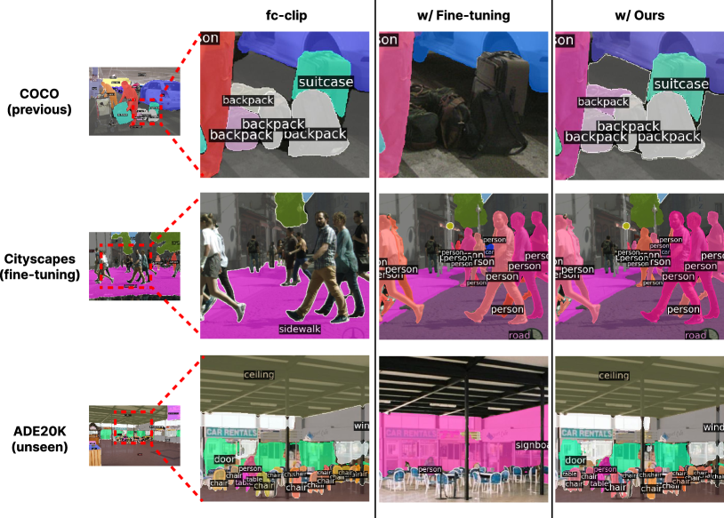
Figure 8: We provide a qualitative analysis on COCO, Cityscapes, and ADE20K. The comparison involves three methods: fc-clip, fine-tuning, and our approach. Both fine-tuning and our method use the Cityscapes dataset to fine-tune fc-clip.

5.4 Qualitative Results

This section provides an analysis of the qualitative results from the original fc-clip, the standard fine-tuning technique, and the proposed method. Figure 8 shows the output of each method. When evaluated on the previous training dataset, the standard fine-tuning technique fails to recognize the backpack, losing information from the previous training dataset. On the fine-tuning dataset, the original fc-clip fails to identify key elements such as road and person. This highlights that OVS models perform well only within the domain of the previous training dataset. When evaluated on the unseen dataset, the standard fine-tuning technique fails to recognize ceiling, a class that does not exist in both the previous training dataset and the fine-tuning dataset. In contrast, the proposed method successfully identifies both previous and newly learned classes, as well as classes not present in either training dataset.

6 Limitations

Our method generates unique model weights for each input sample, which makes it challenging to use when the batch size exceeds one. This limitation is also observed in other continual learning approaches (Wang et al., 2022a; Smith et al., 2023; Jin et al., 2023). One potential solution is to apply parallel processing only during the encoder stage. The encoder stage of OVS models generally requires significant computational resources. However, since our method focuses on decoder weight interpolation, multiple samples can be processed in parallel during the encoder stage. Afterward, the embeddings from each sample can be passed through decoders with different weights. While this approach resolves the batch size limitation, the increased computational cost in the decoder stage remains a concern compared to traditional OVS models. To address this issue, further research is needed to develop a parallel processing mechanism for our method.

7 Conclusion

Conventional segmentation models are limited to recognizing predefined classes, which highlights the growing importance of Open-vocabulary Segmentation (OVS) for broader category prediction. However, OVS models show reduced performance when applied to unseen datasets beyond the previous training dataset. While fine-tuning OVS models improves performance on new datasets, we observe that it leads to catastrophic forgetting of previous knowledge. To address this issue, we propose a method that adaptively interpolates between the weights of the pre-trained decoder and the fine-tuned decoders based on the input sample’s proximity to different domains. We conduct extensive experiments to verify the method, showing that it allows OVS models to effectively learn on new domains while preserving prior knowledge.

Appendix A Appendix

Table A1: Performance comparison between original fine-tuning, previous continual learning methods, and our method. All methods fine-tune the models using Cityscapes. We use PQ, mAP, mIoU for evaluation metrics.

		COCO (previous training)				Cityscapes (fine-tuning)				ADE20K (unseen)
Method	Fine-tuning Dataset	PQ	mAP	mIoU	Avg	PQ	mAP	mIoU	Avg	PQ	mAP	mIoU	Avg
fc-clip	-	50.1	41.1	52.0	47.7	44.0	26.8	56.2	42.4	23.5	17.1	30.4	23.7
+ Fine-tuning		-22.7	-16.2	-11.8	-16.9	+20.1	+13.9	+21.2	+18.4	-10.3	-6.3	-3.9	-6.8
+ ER		-1.6	-2.7	+0.2	-1.4	+19.0	+13.0	+20.1	+17.4	+0.3	-3.5	+0.9	-0.8
+ LwF		-10.7	-11.9	-7.9	-10.2	+12.2	+2.7	+10.2	+8.3	-0.8	-5.4	+0.8	-1.8
+ EWC		-25.9	-19.0	-13.3	-19.4	+19.3	+11.2	+18.4	+16.3	-9.8	-8.4	-4.2	-7.5
+ ECLIPSE		-6.0	-6.2	-3.9	-5.3	+2.2	+0.2	+4.3	+2.2	+0.9	-3.6	+2.0	-0.3
+ Ours	Cityscapes	+0.3	+0.5	+0.1	+0.3	+20.2	+13.9	+21.3	+18.5	+2.5	-1.2	+2.5	+1.3
X-Decoder	-	56.7	46.9	67.4	57.0	36.3	25.4	52.9	38.2	16.7	11.7	24.9	17.8
+ Fine-tuning		-50.4	-32.2	-53.7	-45.5	+26.6	+11.7	+26.7	+21.7	-12.9	-8.1	-19.7	-13.5
+ Ours	Cityscapes	-0.4	-0.4	-0.3	-0.3	+26.6	+11.6	+26.7	+21.7	+0.1	+0.5	-0.3	+0.1

Table A2: Performance comparison between original fine-tuning, previous continual learning methods, and our method. All methods fine-tune the models using ADE20K. We use PQ, mAP, mIoU for evaluation metrics.

		COCO (previous training)				ADE20k (fine-tuning)				Cityscapes (unseen)
Method	Fine-tuning Dataset	PQ	mAP	mIoU	Avg	PQ	mAP	mIoU	Avg	PQ	mAP	mIoU	Avg
fc-clip	-	50.1	41.1	52.0	47.7	23.5	17.1	30.4	23.7	44.0	26.8	56.2	42.4
+ Fine-tuning		-7.7	-6.2	-2.7	-5.5	+24.1	+19.0	+22.0	+21.7	-3.0	-2.8	+2.9	-1.0
+ ER		+0.4	-0.3	+2.9	+1.0	+21.5	+16.3	+19.5	+19.1	-3.5	-2.8	-1.0	-2.4
+ LwF		-3.8	-7.1	-2.4	-4.4	+13.7	+8.4	+11.3	+11.1	-1.0	-6.2	-3.0	-3.4
+ EWC		-11.1	-9.3	-6.0	-8.8	+20.7	+16.2	+18.0	+18.3	-2.6	-3.2	+0.3	-1.8
+ ECLIPSE		-0.5	-1.2	+0.6	-0.3	+0.2	-0.3	+3.0	+1.0	-5.9	-4.0	-2.2	-4.0
+ Ours	ADE20K	+1.7	+1.4	+3.2	+2.1	+23.8	+18.6	+21.1	+21.2	-0.3	-0.7	+0.6	-0.1
X-Decoder	-	56.7	46.9	67.4	57.0	16.7	11.7	24.9	17.8	36.3	25.4	52.9	38.2
+ Fine-tuning		-37.3	-33.6	-42.4	-37.8	+28.2	+18.6	+27.2	+24.6	-3.7	-9.4	-0.8	-4.6
+ Ours	ADE20K	-1.5	-1.7	-1.1	-1.4	+29.2	+19.0	+27.5	+25.2	+1.4	-6.4	+3.5	-0.5

Table A3: Performance comparison between standard fine-tuning and our method. The underlined values indicate the best score for each dataset. We use PQ, mAP, mIoU for evaluation metrics.

		COCO (previous)			ADE20k (fine-tuning 1)			Cityscapes (fine-tuning 2)
Method	The order of fine-tuning	PQ	mAP	mIoU	PQ	mAP	mIoU	PQ	mAP	mIoU
fc-clip	-	50.1	41.1	52.0	23.5	17.1	30.4	44.0	26.8	56.2
+ Fine-tuning	ADE20k → Cityscapes	20.8	19.5	40.0	15.4	14.2	34.9	65.2	42.3	77.6
+ Fine-tuning	Cityscapes → ADE20k	39.3	32.4	48.3	48.3	36.3	52.1	46.0	26.4	61.5
+ Ours	Cityscapes, ADE20k	51.6	42.5	55.3	47.0	35.9	51.4	64.3	40.7	77.6

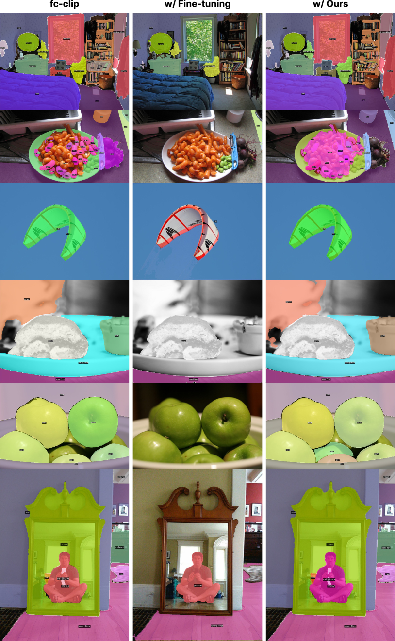
Figure A1: We provide additional qualitative analysis on COCO (previous training dataset). The comparison involves three methods: fc-clip, fine-tuning, and our approach. Fine-tuning and our method both use the Cityscapes dataset to fine-tune fc-clip.

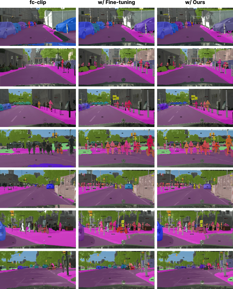
Figure A2: We provide additional qualitative analysis on Cityscapes (fine-tuning dataset). The comparison involves three methods: fc-clip, fine-tuning, and our approach. Fine-tuning and our method both use the Cityscapes dataset to fine-tune fc-clip.

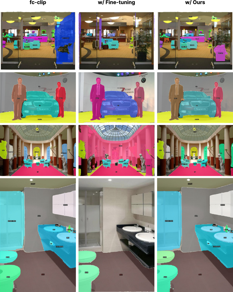
Figure A3: We provide additional qualitative analysis on ADE20K (unseen dataset). The comparison involves three methods: fc-clip, fine-tuning, and our approach. Fine-tuning and our method both use the Cityscapes dataset to fine-tune fc-clip.

References

- Cai et al. (2020) Han Cai, Chuang Gan, Ligeng Zhu, and Song Han. Tinytl: Reduce memory, not parameters for efficient on-device learning. Advances in Neural Information Processing Systems, 33:11285–11297, 2020.
- Chaudhry et al. (2019) Arslan Chaudhry, Marcus Rohrbach, Mohamed Elhoseiny, Thalaiyasingam Ajanthan, Puneet K Dokania, Philip HS Torr, and Marc’Aurelio Ranzato. On tiny episodic memories in continual learning. arXiv preprint arXiv:1902.10486, 2019.
- Chen & Liu (2022) Zhiyuan Chen and Bing Liu. Lifelong machine learning. Springer Nature, 2022.
- Cheng et al. (2022) Bowen Cheng, Ishan Misra, Alexander G Schwing, Alexander Kirillov, and Rohit Girdhar. Masked-attention mask transformer for universal image segmentation. In Proceedings of the IEEE/CVF conference on computer vision and pattern recognition, pp. 1290–1299, 2022.
- Cordts et al. (2016) Marius Cordts, Mohamed Omran, Sebastian Ramos, Timo Rehfeld, Markus Enzweiler, Rodrigo Benenson, Uwe Franke, Stefan Roth, and Bernt Schiele. The cityscapes dataset for semantic urban scene understanding. In Proceedings of the IEEE conference on computer vision and pattern recognition, pp. 3213–3223, 2016.
- Dhar et al. (2019) Prithviraj Dhar, Rajat Vikram Singh, Kuan-Chuan Peng, Ziyan Wu, and Rama Chellappa. Learning without memorizing. In Proceedings of the IEEE/CVF conference on computer vision and pattern recognition, pp. 5138–5146, 2019.
- Ding et al. (2022) Jian Ding, Nan Xue, Gui-Song Xia, and Dengxin Dai. Decoupling zero-shot semantic segmentation. In Proceedings of the IEEE/CVF Conference on Computer Vision and Pattern Recognition, pp. 11583–11592, 2022.
- Everingham et al. (2010) Mark Everingham, Luc Van Gool, Christopher KI Williams, John Winn, and Andrew Zisserman. The pascal visual object classes (voc) challenge. International journal of computer vision, 88:303–338, 2010.
- Ghiasi et al. (2022) Golnaz Ghiasi, Xiuye Gu, Yin Cui, and Tsung-Yi Lin. Scaling open-vocabulary image segmentation with image-level labels. In European Conference on Computer Vision, pp. 540–557. Springer, 2022.
- Gupta et al. (2019) Agrim Gupta, Piotr Dollar, and Ross Girshick. Lvis: A dataset for large vocabulary instance segmentation. In Proceedings of the IEEE/CVF conference on computer vision and pattern recognition, pp. 5356–5364, 2019.
- Houlsby et al. (2019) Neil Houlsby, Andrei Giurgiu, Stanislaw Jastrzebski, Bruna Morrone, Quentin De Laroussilhe, Andrea Gesmundo, Mona Attariyan, and Sylvain Gelly. Parameter-efficient transfer learning for nlp. In International conference on machine learning, pp. 2790–2799. PMLR, 2019.
- Hu et al. (2021) Edward J Hu, Yelong Shen, Phillip Wallis, Zeyuan Allen-Zhu, Yuanzhi Li, Shean Wang, Lu Wang, and Weizhu Chen. Lora: Low-rank adaptation of large language models. arXiv preprint arXiv:2106.09685, 2021.
- Ilharco et al. (2022) Gabriel Ilharco, Marco Tulio Ribeiro, Mitchell Wortsman, Suchin Gururangan, Ludwig Schmidt, Hannaneh Hajishirzi, and Ali Farhadi. Editing models with task arithmetic. arXiv preprint arXiv:2212.04089, 2022.
- Iscen et al. (2020) Ahmet Iscen, Jeffrey Zhang, Svetlana Lazebnik, and Cordelia Schmid. Memory-efficient incremental learning through feature adaptation. In Computer Vision–ECCV 2020: 16th European Conference, Glasgow, UK, August 23–28, 2020, Proceedings, Part XVI 16, pp. 699–715. Springer, 2020.
- Jia et al. (2022) Menglin Jia, Luming Tang, Bor-Chun Chen, Claire Cardie, Serge Belongie, Bharath Hariharan, and Ser-Nam Lim. Visual prompt tuning. In European Conference on Computer Vision, pp. 709–727. Springer, 2022.
- Jin et al. (2023) Hyundong Jin, Gyeong-hyeon Kim, Chanho Ahn, and Eunwoo Kim. Growing a brain with sparsity-inducing generation for continual learning. In Proceedings of the IEEE/CVF International Conference on Computer Vision, pp. 18961–18970, 2023.
- Johnson & Khoshgoftaar (2019) Justin M Johnson and Taghi M Khoshgoftaar. Survey on deep learning with class imbalance. Journal of big data, 6(1):1–54, 2019.
- Kim et al. (2024) Beomyoung Kim, Joonsang Yu, and Sung Ju Hwang. Eclipse: Efficient continual learning in panoptic segmentation with visual prompt tuning. In Proceedings of the IEEE/CVF Conference on Computer Vision and Pattern Recognition, pp. 3346–3356, 2024.
- Kirillov et al. (2019) Alexander Kirillov, Kaiming He, Ross Girshick, Carsten Rother, and Piotr Dollár. Panoptic segmentation. In Proceedings of the IEEE/CVF conference on computer vision and pattern recognition, pp. 9404–9413, 2019.
- Kirillov et al. (2023) Alexander Kirillov, Eric Mintun, Nikhila Ravi, Hanzi Mao, Chloe Rolland, Laura Gustafson, Tete Xiao, Spencer Whitehead, Alexander C Berg, Wan-Yen Lo, et al. Segment anything. In Proceedings of the IEEE/CVF International Conference on Computer Vision, pp. 4015–4026, 2023.
- Kirkpatrick et al. (2017) James Kirkpatrick, Razvan Pascanu, Neil Rabinowitz, Joel Veness, Guillaume Desjardins, Andrei A Rusu, Kieran Milan, John Quan, Tiago Ramalho, Agnieszka Grabska-Barwinska, et al. Overcoming catastrophic forgetting in neural networks. Proceedings of the national academy of sciences, 114(13):3521–3526, 2017.
- Kornblith et al. (2019) Simon Kornblith, Jonathon Shlens, and Quoc V Le. Do better imagenet models transfer better? In Proceedings of the IEEE/CVF conference on computer vision and pattern recognition, pp. 2661–2671, 2019.
- Krishna et al. (2017) Ranjay Krishna, Yuke Zhu, Oliver Groth, Justin Johnson, Kenji Hata, Joshua Kravitz, Stephanie Chen, Yannis Kalantidis, Li-Jia Li, David A Shamma, et al. Visual genome: Connecting language and vision using crowdsourced dense image annotations. International journal of computer vision, 123:32–73, 2017.
- Li et al. (2022) Boyi Li, Kilian Q Weinberger, Serge Belongie, Vladlen Koltun, and René Ranftl. Language-driven semantic segmentation. arXiv preprint arXiv:2201.03546, 2022.
- Li & Hoiem (2017) Zhizhong Li and Derek Hoiem. Learning without forgetting. IEEE transactions on pattern analysis and machine intelligence, 40(12):2935–2947, 2017.
- Liang & Li (2024) Yan-Shuo Liang and Wu-Jun Li. Inflora: Interference-free low-rank adaptation for continual learning. In Proceedings of the IEEE/CVF Conference on Computer Vision and Pattern Recognition, pp. 23638–23647, 2024.
- Lin et al. (2014) Tsung-Yi Lin, Michael Maire, Serge Belongie, James Hays, Pietro Perona, Deva Ramanan, Piotr Dollár, and C Lawrence Zitnick. Microsoft coco: Common objects in context. In Computer Vision–ECCV 2014: 13th European Conference, Zurich, Switzerland, September 6-12, 2014, Proceedings, Part V 13, pp. 740–755. Springer, 2014.
- Liu et al. (2018) Xialei Liu, Marc Masana, Luis Herranz, Joost Van de Weijer, Antonio M Lopez, and Andrew D Bagdanov. Rotate your networks: Better weight consolidation and less catastrophic forgetting. In 2018 24th International Conference on Pattern Recognition (ICPR), pp. 2262–2268. IEEE, 2018.
- Liu et al. (2022) Zhuang Liu, Hanzi Mao, Chao-Yuan Wu, Christoph Feichtenhofer, Trevor Darrell, and Saining Xie. A convnet for the 2020s. In Proceedings of the IEEE/CVF conference on computer vision and pattern recognition, pp. 11976–11986, 2022.
- Lopez-Paz & Ranzato (2017) David Lopez-Paz and Marc’Aurelio Ranzato. Gradient episodic memory for continual learning. Advances in neural information processing systems, 30, 2017.
- Mottaghi et al. (2014) Roozbeh Mottaghi, Xianjie Chen, Xiaobai Liu, Nam-Gyu Cho, Seong-Whan Lee, Sanja Fidler, Raquel Urtasun, and Alan Yuille. The role of context for object detection and semantic segmentation in the wild. In IEEE Conference on Computer Vision and Pattern Recognition (CVPR), 2014.
- Mundt et al. (2023) Martin Mundt, Yongwon Hong, Iuliia Pliushch, and Visvanathan Ramesh. A wholistic view of continual learning with deep neural networks: Forgotten lessons and the bridge to active and open world learning. Neural Networks, 160:306–336, 2023.
- Neuhold et al. (2017) Gerhard Neuhold, Tobias Ollmann, Samuel Rota Bulo, and Peter Kontschieder. The mapillary vistas dataset for semantic understanding of street scenes. In Proceedings of the IEEE international conference on computer vision, pp. 4990–4999, 2017.
- Ordonez et al. (2011) Vicente Ordonez, Girish Kulkarni, and Tamara Berg. Im2text: Describing images using 1 million captioned photographs. Advances in neural information processing systems, 24, 2011.
- Parisi et al. (2019) German I Parisi, Ronald Kemker, Jose L Part, Christopher Kanan, and Stefan Wermter. Continual lifelong learning with neural networks: A review. Neural networks, 113:54–71, 2019.
- Qiao et al. (2023) Jingyang Qiao, Xin Tan, Chengwei Chen, Yanyun Qu, Yong Peng, Yuan Xie, et al. Prompt gradient projection for continual learning. In The Twelfth International Conference on Learning Representations, 2023.
- Radford et al. (2021) Alec Radford, Jong Wook Kim, Chris Hallacy, Aditya Ramesh, Gabriel Goh, Sandhini Agarwal, Girish Sastry, Amanda Askell, Pamela Mishkin, Jack Clark, et al. Learning transferable visual models from natural language supervision. In International conference on machine learning, pp. 8748–8763. PMLR, 2021.
- Ritter et al. (2018) Hippolyt Ritter, Aleksandar Botev, and David Barber. Online structured laplace approximations for overcoming catastrophic forgetting. Advances in Neural Information Processing Systems, 31, 2018.
- Rypeść et al. (2024) Grzegorz Rypeść, Sebastian Cygert, Valeriya Khan, Tomasz Trzciński, Bartosz Zieliński, and Bartłomiej Twardowski. Divide and not forget: Ensemble of selectively trained experts in continual learning. arXiv preprint arXiv:2401.10191, 2024.
- Shin et al. (2017) Hanul Shin, Jung Kwon Lee, Jaehong Kim, and Jiwon Kim. Continual learning with deep generative replay. Advances in neural information processing systems, 30, 2017.
- Smith et al. (2023) James Seale Smith, Leonid Karlinsky, Vyshnavi Gutta, Paola Cascante-Bonilla, Donghyun Kim, Assaf Arbelle, Rameswar Panda, Rogerio Feris, and Zsolt Kira. Coda-prompt: Continual decomposed attention-based prompting for rehearsal-free continual learning. In Proceedings of the IEEE/CVF Conference on Computer Vision and Pattern Recognition, pp. 11909–11919, 2023.
- Wang et al. (2024a) Haoxiang Wang, Pavan Kumar Anasosalu Vasu, Fartash Faghri, Raviteja Vemulapalli, Mehrdad Farajtabar, Sachin Mehta, Mohammad Rastegari, Oncel Tuzel, and Hadi Pouransari. Sam-clip: Merging vision foundation models towards semantic and spatial understanding. In Proceedings of the IEEE/CVF Conference on Computer Vision and Pattern Recognition, pp. 3635–3647, 2024a.
- Wang et al. (2024b) Liyuan Wang, Xingxing Zhang, Hang Su, and Jun Zhu. A comprehensive survey of continual learning: theory, method and application. IEEE Transactions on Pattern Analysis and Machine Intelligence, 2024b.
- Wang et al. (2022a) Yabin Wang, Zhiwu Huang, and Xiaopeng Hong. S-prompts learning with pre-trained transformers: An occam’s razor for domain incremental learning. Advances in Neural Information Processing Systems, 35:5682–5695, 2022a.
- Wang et al. (2022b) Zifeng Wang, Zizhao Zhang, Sayna Ebrahimi, Ruoxi Sun, Han Zhang, Chen-Yu Lee, Xiaoqi Ren, Guolong Su, Vincent Perot, Jennifer Dy, et al. Dualprompt: Complementary prompting for rehearsal-free continual learning. In European Conference on Computer Vision, pp. 631–648. Springer, 2022b.
- Wang et al. (2022c) Zifeng Wang, Zizhao Zhang, Chen-Yu Lee, Han Zhang, Ruoxi Sun, Xiaoqi Ren, Guolong Su, Vincent Perot, Jennifer Dy, and Tomas Pfister. Learning to prompt for continual learning. In Proceedings of the IEEE/CVF conference on computer vision and pattern recognition, pp. 139–149, 2022c.
- Wortsman et al. (2022) Mitchell Wortsman, Gabriel Ilharco, Samir Ya Gadre, Rebecca Roelofs, Raphael Gontijo-Lopes, Ari S Morcos, Hongseok Namkoong, Ali Farhadi, Yair Carmon, Simon Kornblith, et al. Model soups: averaging weights of multiple fine-tuned models improves accuracy without increasing inference time. In International conference on machine learning, pp. 23965–23998. PMLR, 2022.
- Wu et al. (2023) Size Wu, Wenwei Zhang, Lumin Xu, Sheng Jin, Xiangtai Li, Wentao Liu, and Chen Change Loy. Clipself: Vision transformer distills itself for open-vocabulary dense prediction. arXiv preprint arXiv:2310.01403, 2023.
- Xu et al. (2023) Jiarui Xu, Sifei Liu, Arash Vahdat, Wonmin Byeon, Xiaolong Wang, and Shalini De Mello. Open-vocabulary panoptic segmentation with text-to-image diffusion models. In Proceedings of the IEEE/CVF Conference on Computer Vision and Pattern Recognition, pp. 2955–2966, 2023.
- Xu et al. (2024) Jingxuan Xu, Wuyang Chen, Yao Zhao, and Yunchao Wei. Transferable and principled efficiency for open-vocabulary segmentation. In Proceedings of the IEEE/CVF Conference on Computer Vision and Pattern Recognition, pp. 15814–15824, 2024.
- Yang et al. (2022) Jianwei Yang, Chunyuan Li, Xiyang Dai, and Jianfeng Gao. Focal modulation networks. Advances in Neural Information Processing Systems, 35:4203–4217, 2022.
- Yosinski et al. (2014) Jason Yosinski, Jeff Clune, Yoshua Bengio, and Hod Lipson. How transferable are features in deep neural networks? Advances in neural information processing systems, 27, 2014.
- Yu et al. (2020) Fisher Yu, Haofeng Chen, Xin Wang, Wenqi Xian, Yingying Chen, Fangchen Liu, Vashisht Madhavan, and Trevor Darrell. Bdd100k: A diverse driving dataset for heterogeneous multitask learning. In Proceedings of the IEEE/CVF conference on computer vision and pattern recognition, pp. 2636–2645, 2020.
- Yu et al. (2024) Qihang Yu, Ju He, Xueqing Deng, Xiaohui Shen, and Liang-Chieh Chen. Convolutions die hard: Open-vocabulary segmentation with single frozen convolutional clip. Advances in Neural Information Processing Systems, 36, 2024.
- Yuan et al. (2024) Haobo Yuan, Xiangtai Li, Chong Zhou, Yining Li, Kai Chen, and Chen Change Loy. Open-vocabulary sam: Segment and recognize twenty-thousand classes interactively. arXiv preprint arXiv:2401.02955, 2024.
- Zhou et al. (2019) Bolei Zhou, Hang Zhao, Xavier Puig, Tete Xiao, Sanja Fidler, Adela Barriuso, and Antonio Torralba. Semantic understanding of scenes through the ade20k dataset. International Journal of Computer Vision, 127:302–321, 2019.
- Zhou et al. (2022) Chong Zhou, Chen Change Loy, and Bo Dai. Extract free dense labels from clip. In European Conference on Computer Vision, pp. 696–712. Springer, 2022.
- Zou et al. (2023a) Xueyan Zou, Zi-Yi Dou, Jianwei Yang, Zhe Gan, Linjie Li, Chunyuan Li, Xiyang Dai, Harkirat Behl, Jianfeng Wang, Lu Yuan, et al. Generalized decoding for pixel, image, and language. In Proceedings of the IEEE/CVF Conference on Computer Vision and Pattern Recognition, pp. 15116–15127, 2023a.
- Zou et al. (2023b) Xueyan Zou, Linjie Li, Jianfeng Wang, Jianwei Yang, Mingyu Ding, Zhengyuan Yang, Feng Li, Hao Zhang, Shilong Liu, Arul Aravinthan, et al. Interfacing foundation models’ embeddings. arXiv preprint arXiv:2312.07532, 2023b.
- Zou et al. (2024) Xueyan Zou, Jianwei Yang, Hao Zhang, Feng Li, Linjie Li, Jianfeng Wang, Lijuan Wang, Jianfeng Gao, and Yong Jae Lee. Segment everything everywhere all at once. Advances in Neural Information Processing Systems, 36, 2024.