Renormalization group running effects in $pp\to t\bar{t}h$ in the SMEFT

Abstract

We analyze the effects of renormalization group running of the Wilson coefficients in the SMEFT in the context of single Higgs production in association with a top-antitop pair. In particular, we analyze the differential cross section with respect to the Higgs trasnverse momentum. We extend the usual $\mathcal{O}\left(\alpha_{s}\right)$ analysis including also the top Yukawa running effects, whose impact can be significant when large Wilson coefficients are considered. We employ a dynamical and a fixed renormalization scale with different set-ups for the Wilson coefficients, defined at the TeV scale. Additionally, we comment on the accuracy of the widely-used first leading-logarithm approximation.

1 Introduction

The Standard Model of particle physics (SM) stands as one of the most important scientific achievements of the recent time. Despite that, several observations and theoretical puzzles suggest that it should be extended. So far, no clear evidence for New Physics (NP) has been observed. Additionally, it will not be possible to explore higher energy regions in the near future, diminuishing the chances of direct observation of new degrees of freedom.

Effective Field Theories (EFTs) represent a general and efficient framework to parametrize small deviations from the SM, allowing for global analyses combining data from different experiments. Here, we employ the Standard Model Effective Field Theory (SMEFT), which extends the SM Lagrangian with a series of higher-dimensional operators $\mathcal{O}_{i}$. The aforementioned operators contain SM fields only and must be invariant under the unbroken SM gauge group, namely $\mathbf{SU(3)}_{\mathrm{C}}\otimes\mathbf{SU(2)}_{\mathrm{L}}\otimes\mathbf{U(1)}_{\mathrm{Y}}$. We have:

$$\mathcal{L}_{\textrm{SMEFT}}=\mathcal{L}_{\textrm{SM}}+\sum_{\mathfrak{D}_{i}>4}\frac{\mathcal{C}_{i}}{\Lambda^{\mathfrak{D}_{i}-4}}\mathcal{O}_{i},$$ (1)

where $\mathfrak{D}_{i}$ denotes the dimension of $\mathcal{O}_{i}$ in units of energy. The Wilson coefficients $\mathcal{C}_{i}$ in Eq. (1) capture the impact of heavy BSM particles having masses $\Lambda$, with $\Lambda\gg v=246\,\mathrm{GeV}$. Under the assumption of conservation of baryon and lepton number, the first term in the expansion has $\mathfrak{D}=6$. A complete and non-redundant basis at this order is the so-called Warsaw basis [2], consisting in 2499 independent operators in the most flavor-agnostic scenario. Already at this order, a plethora of new interactions arise [3], changing significantly the SM phenomenology.

2 Running effects

The precision obtained by current experimental measurements often requires higher order computations involving loop diagrams, which typically diverge. The renormalization procedure provides a strategy to eliminate the divergencies from on-shell matrix elements, providing finite and well-defined physical predictions. As a consequence, it induces an energy-scale dependence in the parameters of the theory, described by a system of coupled differential equations which go under the name of Renormalization Group Equations (RGEs). At dimension-six, the RGEs must be linear, allowing to write them as

$$\mu\frac{d\mathcal{C}_{i}(\mu)}{d\mu}=\frac{1}{16\pi^{2}}{\color[rgb]{0,0,0}{\Gamma_{ij}(\mu)}\mathcal{C}_{j}(\mu)},$$ (2)

where we introduced $\Gamma$, known as Anomalous Dimension Matrix (ADM). The one-loop results are fully known [4, 5, 6] and some partial results at two-loop level are available in [7, 8, 9, 10, 11, 12].

The energy-scale dependence of the ADM is fully contained in the couplings, allowing to decompose it as $\Gamma_{ij}(\mu)$ $=g_{1}^{2}(\mu)\Gamma_{ij}^{(g_{1}^{2})}$ $+g_{2}^{2}(\mu)\Gamma_{ij}^{(g_{2}^{2})}+\ldots,$ where the matrices $\Gamma_{ij}^{(g_{i}^{2})}$ are constant. Neglecting all the terms apart from the strong coupling provides an exactly solvable system, which represent the most used approach in the inclusion of running effects [13, 14, 15, 16, 17, 18].

If additional interactions are considered, an analytic solution is not possible. The RGEs must be solved either numerically or by employing an approximation, for example via the first leading-logarithm solution:

$${\color[rgb]{0,0,0}\mathcal{C}_{i}(\mu_{\textrm{F}})}={\color[rgb]{0,0,0}\mathcal{C}_{i}(\mu_{\textrm{I}})}+{\color[rgb]{0,0,0}\Gamma_{ij}(\mu_{\textrm{I}})\mathcal{C}_{j}(\mu_{\textrm{I}})}\frac{\log{\left({\color[rgb]{0,0,0}\mu_{\textrm{F}}}/{\color[rgb]{0,0,0}\mu_{\textrm{I}}}\right)}}{16\pi^{2}}.$$ (3)

This method is simple and fast, but it is reliable only if the energy scales $\mu_{\textrm{F}},\,\mu_{\textrm{I}}$ are close.

3 Implementation and results

Higgs production in association with a top-antitop pair arises at tree-level in the SM, see Fig. 1. We consider only SMEFT operators which enter at tree-level, see Fig. 2.

(a)

(b)

(c)

(d)

Figure 1: Tree-level diagrams for $pp\to t\bar{t}h$ in the SM.

(a)

(b)

(c)

(d)

Figure 2: Tree-level diagrams for $pp\to t\bar{t}h$ in the SMEFT. The colored square dots denote insertions of SMEFT operators.

To assess the impact of the running effects, we set some non-vanishing Wilson coefficients at $\Lambda=2\;\text{TeV}$ and we run them to the renormalization scale $\mu_{\mathrm{R}}$ using RGESolver [19]. We repeat the computation with two different renormalization scales: a fixed scale $\mu_{\mathrm{R}}=m_{t}$ (same for all the events) and a dynamical scale $\mu_{\mathrm{R}}=(p_{T,h}+p_{T,t}+p_{T,\bar{t}})/2$ (differs event by event). Understanding if the usage of a fixed renormalization scale is a valid approximation is crucial, due to the technical difficulties associated to the numeric solution of the RGEs.

We compare two scenarios: we employ the conservative $\mathcal{O}\left(1/\Lambda^{4}\right)$ bounds and the extreme $\mathcal{O}\left(1/\Lambda^{2}\right)$ bounds from [20], showing the results in Figs. 4, 4. We observe a difference between the two renormalization scale choices up to 25% in the first case, increasing to 70% in the latter.

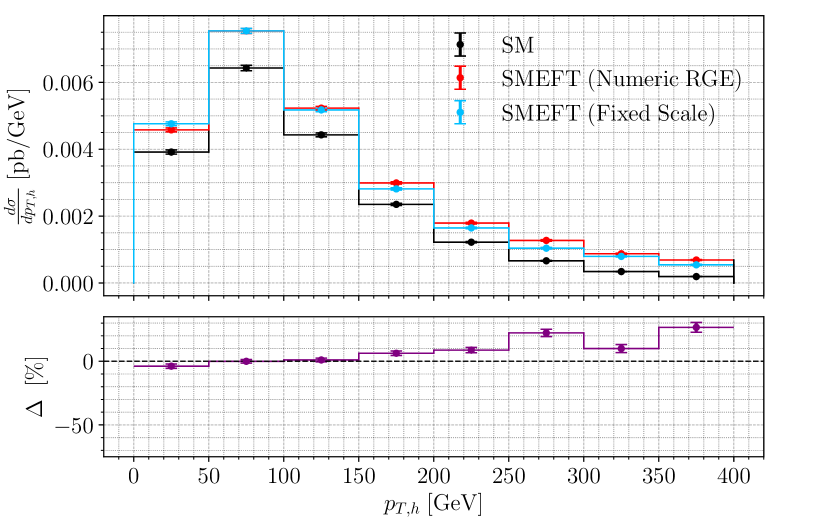
Figure 3: Higgs transverse momentum distribution in the conservative scenario, dynamical vs fixed renormalization scale.

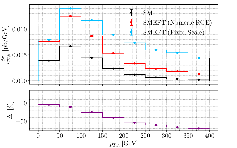
Figure 4: Higgs transverse momentum distribution in the extreme scenario, dynamical vs fixed renormalization scale.

We have compared the numeric solution of the RGEs with the first leading-logarithm approximation in Eq. (3), observing negliglible differences between the two in the conservative scenario in Fig. 6, with instead discrepancies up to 15% in the extreme case in Fig. 6.

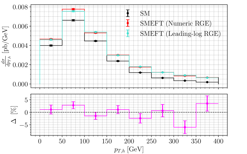
Figure 5: Higgs transverse momentum distribution in the conservative scenario, numeric vs leading-logarithm running.

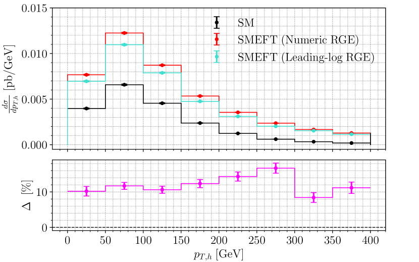
Figure 6: Higgs transverse momentum distribution in the extreme scenario, numeric vs leading-logarithm running.

We studied the differential distribution with respect to the Higgs transverse momentum considering individually the two four-top operators $\mathcal{O}_{Qt}^{(1,8)}=\left(\bar{Q}_{L}\gamma^{\mu}(T^{A})Q_{L}\right)\left(\bar{t}_{R}\gamma_{\mu}(T^{A})t_{R}\right)$ in Figs. 10, 10. Their contribution to $g_{ht\bar{t}}$ , the effective Higgs-top coupling, goes as $y_{t}^{3}\left(\mathcal{C}_{Qt}^{(1)}+\frac{4}{3}\mathcal{C}_{Qt}^{(8)}\right)$, providing a similar behaviour within both scenarios, see Figs. 10, 10. Instead, their strong mixing with other operators entering in $pp\to\bar{t}th$ at tree-level is different, due to the different color structure.

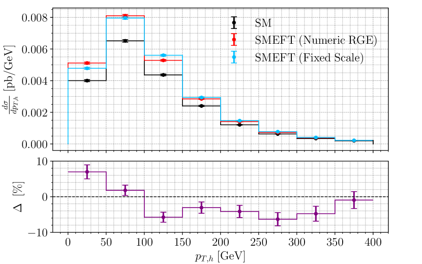
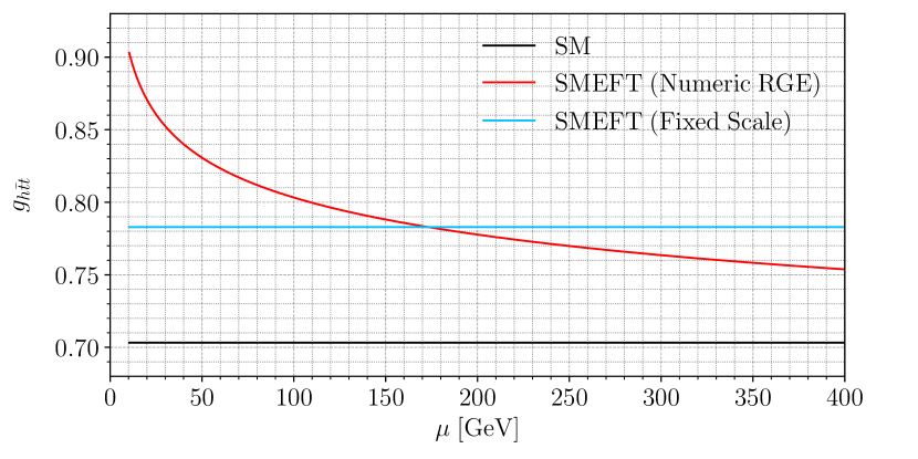
Figure 7: Higgs transverse momentum distribution with $\mathcal{C}_{Qt}^{(1)}(\Lambda)=\frac{4}{3}\times 20\,/\mathrm{TeV}^{2}$.

Figure 8: Running of $g_{ht\bar{t}}$ with $\mathcal{C}_{Qt}^{(1)}(\Lambda)=\frac{4}{3}\times 20\,/\mathrm{TeV}^{2}$.

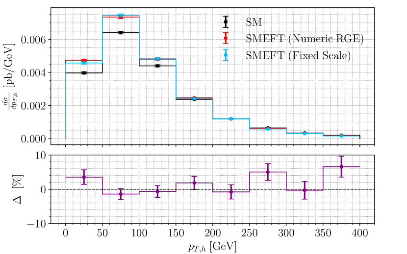
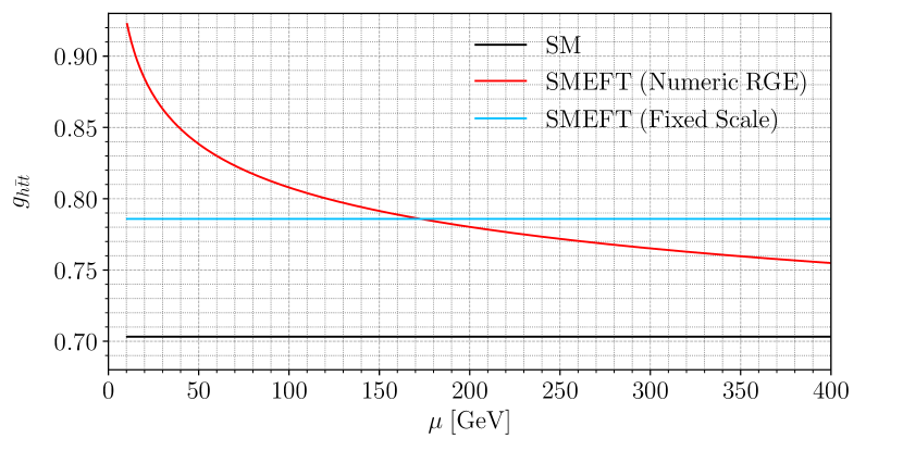
Figure 9: Higgs transverse momentum distribution with $\mathcal{C}_{Qt}^{(8)}(\Lambda)=20\,/\mathrm{TeV}^{2}$.

Figure 10: Running of $g_{ht\bar{t}}$ with $\mathcal{C}_{Qt}^{(8)}(\Lambda)=20\,/\mathrm{TeV}^{2}$.

By observing that there is a sizeable difference between dynamical and fixed renormalization scales in both cases, we conclude that top-Yukawa running effects can be relevant in presence of large Wilson coefficients, advocating for their inclusion together with effects proportional to the strong coupling.

4 Conclusions and outlook

Running effects are expected to become more and more relevant in the near future, due to the increasing precision at the experimental and theoretical level. We have discussed that relevant differences can arise when employing a dynamical renormalization scale with respect to a fixed renormalization scale by analyzing the transverse momentum spectrum in single Higgs production in association with a top-antitop pair. Additionally, we have observed that the widely-used leading-logarithm approximation in the solution of the RGEs departures sizeably from the numeric one in presence of large Wilson coefficients. Finally, we showed how Yukawa contributions can be as relevant as strong ones in some scenarios, highlighting the importance of their inclusion in phenomenological studies.

References

- [1] Stefano Di Noi and Ramona Gröber. Renormalisation group running effects in in the Standard Model Effective Field Theory. Eur. Phys. J. C, 84(4):403, 2024.
- [2] B. Grzadkowski, M. Iskrzynski, M. Misiak, and J. Rosiek. Dimension-Six Terms in the Standard Model Lagrangian. JHEP, 10:085, 2010.
- [3] A. Dedes, W. Materkowska, M. Paraskevas, J. Rosiek, and K. Suxho. Feynman rules for the Standard Model Effective Field Theory in Rξ -gauges. JHEP, 06:143, 2017.
- [4] Elizabeth E. Jenkins, Aneesh V. Manohar, and Michael Trott. Renormalization Group Evolution of the Standard Model Dimension Six Operators I: Formalism and lambda Dependence. JHEP, 10:087, 2013.
- [5] Elizabeth E. Jenkins, Aneesh V. Manohar, and Michael Trott. Renormalization Group Evolution of the Standard Model Dimension Six Operators II: Yukawa Dependence. JHEP, 01:035, 2014.
- [6] Rodrigo Alonso, Elizabeth E. Jenkins, Aneesh V. Manohar, and Michael Trott. Renormalization Group Evolution of the Standard Model Dimension Six Operators III: Gauge Coupling Dependence and Phenomenology. JHEP, 04:159, 2014.
- [7] Zvi Bern, Julio Parra-Martinez, and Eric Sawyer. Nonrenormalization and Operator Mixing via On-Shell Methods. Phys. Rev. Lett., 124(5):051601, 2020.
- [8] Zvi Bern, Julio Parra-Martinez, and Eric Sawyer. Structure of two-loop SMEFT anomalous dimensions via on-shell methods. JHEP, 10:211, 2020.
- [9] Elizabeth E. Jenkins, Aneesh V. Manohar, Luca Naterop, and Julie Pagès. Two Loop Renormalization of Scalar Theories using a Geometric Approach. 10 2023.
- [10] Stefano Di Noi, Ramona Gröber, Gudrun Heinrich, Jannis Lang, and Marco Vitti. 5 schemes and the interplay of SMEFT operators in the Higgs-gluon coupling. Phys. Rev. D, 109(9):095024, 2024.
- [11] Stefano Di Noi, Ramona Gröber, and Manoj K. Mandal. Two-loop running effects in Higgs physics in Standard Model Effective Field Theory. 8 2024.
- [12] Lukas Born, Javier Fuentes-Martín, Sandra Kvedaraitė, and Anders Eller Thomsen. Two-Loop Running in the Bosonic SMEFT Using Functional Methods. 10 2024.
- [13] Rafael Aoude, Fabio Maltoni, Olivier Mattelaer, Claudio Severi, and Eleni Vryonidou. Renormalisation group effects on SMEFT interpretations of LHC data. JHEP, 09:191, 2023.
- [14] Fabio Maltoni, Giuseppe Ventura, and Eleni Vryonidou. Impact of SMEFT renormalisation group running on Higgs production at the LHC. 6 2024.
- [15] Massimiliano Grazzini, Agnieszka Ilnicka, and Michael Spira. Higgs boson production at large transverse momentum within the SMEFT: analytical results. Eur. Phys. J. C, 78(10):808, 2018.
- [16] Marco Battaglia, Massimiliano Grazzini, Michael Spira, and Marius Wiesemann. Sensitivity to BSM effects in the Higgs pT spectrum within SMEFT. JHEP, 11:173, 2021.
- [17] Fabio Maltoni, Eleni Vryonidou, and Cen Zhang. Higgs production in association with a top-antitop pair in the Standard Model Effective Field Theory at NLO in QCD. JHEP, 10:123, 2016.
- [18] Gudrun Heinrich and Jannis Lang. Renormalisation group effects in SMEFT for di-Higgs production. 9 2024.
- [19] Stefano Di Noi and Luca Silvestrini. RGESolver: a C++ library to perform renormalization group evolution in the Standard Model Effective Theory. Eur. Phys. J. C, 83(3):200, 2023.
- [20] Jacob J. Ethier, Giacomo Magni, Fabio Maltoni, Luca Mantani, Emanuele R. Nocera, Juan Rojo, Emma Slade, Eleni Vryonidou, and Cen Zhang. Combined SMEFT interpretation of Higgs, diboson, and top quark data from the LHC. JHEP, 11:089, 2021.