Electrical Transport in Tunably-Disordered Metamaterials

Abstract

Naturally occurring materials are often disordered, with their bulk properties being challenging to predict from the structure, due to the lack of underlying crystalline axes. In this paper, we develop a digital pipeline from algorithmically-created configurations with tunable disorder to 3D printed materials, as a tool to aid in the study of such materials, using electrical resistance as a test case. The designed material begins with a random point cloud that is iteratively evolved using Lloyd’s algorithm to approach uniformity, with the points being connected via a Delaunay triangulation to form a disordered network metamaterial. Utilizing laser powder bed fusion additive manufacturing with stainless steel 17-4 PH and titanium alloy Ti-6Al-4V, we are able to experimentally measure the bulk electrical resistivity of the disordered network. We found that the graph Laplacian accurately predicts the effective resistance of the structure, but is highly sensitive to anisotropy and global network topology, preventing a single network statistic or disorder characterization from predicting global resistivity.

I Introduction

Research on metamaterials, whether mechanical or photonic, has focused primarily on ordered structures [1, 2, 3, 4, 5, 6], where the bulk properties are inherited from both the constituent material and the connectivity of the lattice. In contrast, the ubiquity of disorder within naturally-occurring materials raises the question of how bulk properties arise when the underlying structure is no longer composed along well-defined crystalline axes. A particularly interesting case is that of hyperuniform structures, for which the density fluctuations grow more slowly than area or volume in the large area or volume limit. Such materials are predicted to thereby have special transport properties [7]. The potential use of off-lattice, disordered metamaterials — as has recently attracted interest [8, 9, 10] — has a key advantage of providing a much larger parameter space to explore than lattices alone can provide.

In order to explore the effects of disorder on transport properties, we consider the test case of electrical resistance within a tunably-disordered network of metal beams (see Fig. 1) created from Lloyd’s algorithm [11]. The choice of electrical resistance provides both a quantity easily measured in the lab, and an exact prediction via the graph Laplacian [12]. When writing the configuration of beams as a network, the edge weights encode the electrical resistance of each beam, which is proportional to its length. Using the graph Laplacian to find an effective resistance, $R_{\textrm{eff}}$, across the entire network is equivalent to solving the full equations (Kirchoff’s laws), which we find is quite sensitive to small configurational changes in the network.

Our numerical tests and physical samples (see Fig. 1) are both created via the same procedure, beginning from a disordered point cloud that is evolved under Lloyd’s algorithm to a more-ordered (approaching hyperuniform [13, 14]) configuration. This allows us to use numerical methods to explore the variability between configurations created by different realizations of the same process, as well as across systems of different sizes. For select configurations, we use laser powder bed fusion additive manufacturing (L-PBF AM) to create physical metal alloy samples [15, 16], providing a validation of the approach.

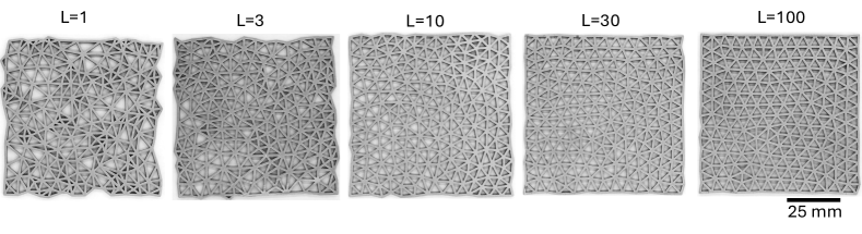
Figure 1: Photos of additively-manufactured Ti-6Al-4V samples created from $N=200$ nodes, subjected to $L=1,3,10,30,100$ iterations of Lloyd’s algorithm. A movie of the evolving point cloud from $L=1$ to $L=100$ is available at [17].

For each configuration, we characterize the disorder via the edge-length distribution, degree distribution, and entropy (degree or edge). We find that the graph Laplacian accurately reproduces the measured effective (bulk) resistance $R_{\textrm{eff}}$ for each printed network with no free parameters, only the known resistivity of the printed material. In addition, the observed variability in $R_{\textrm{eff}}$ within an ensemble of configurations produced under the same protocol is largest for the most disordered systems, which are also those with the largest variance in edge length. In all cases, we observe that the predicted current on specific edges depends both on network topology and the direction of applied voltage, with significant anisotropy present.

II Methods

II.1 Generating configurations

Our tunably-disordered network materials were constructed from point clouds (nodes) that were connected together by edges using a Voronoi tesselation and Delaunay triangulation subjected to multiple iterations of Lloyd’s algorithm [11] to make them progressively more ordered. Five examples, from $L=1$ to $L=100$ iterations, are shown in Fig. 1, each created using the procedure described below.

Each series of related configurations was started by selecting $N$ points drawn from a uniform distribution within a unitless $2000\times 2000$ bounding box. We first generated a Voronoi tessellation which was stored as a list of vertices for each resulting polygon. Following the methods of [18], we truncated this tessellation to the pre-defined bounding box. Rather than ignoring polygon vertices that fell outside the bounding box, we explicitly computed the intersection of the polygons and the bounding box, updating the vertices that now land on the bounding box. We then iteratively performed Lloyd’s algorithm, updating the location of the point cloud points by first calculating the centroid of each Voronoi polygon, and then moving the point cloud point to the centroid location, creating a new point cloud. The first iteration is denoted $L=1$. We then recomputed the new Voronoi tessellation, truncated the polygons, and performed Lloyd’s algorithm again, up to $L=100$ iterations. Our disordered lattices were constructed from the Delaunay triangulation of the point cloud at any step of this process. The Delaunay triangulation connects any two point cloud points if their respective Voronoi polygons share an edge. The code for generating these configurations is available on GitHub [19].

Evolving one initial point cloud through iterations of Lloyd’s algorithm approaches crystallinity [13, 20, 14]. As we will see in Sec. III.1 this change in uniformity happens quickly at first, then progresses approximately logarithmically. In our numerical analyses, we use 20 different initial point clouds at each of $N=100,200,300,$ and $500$, analyzed from $L=0$ (the original point cloud) to 100. In our experiments, we selected one initial point cloud with $N=200$ points, and printed physical samples at iteration counts $L=1$, 3, 10, 30, and 100.

II.2 Sample fabrication

As shown in Fig. 1, we selectively printed one realization of the $N=200$ network configurations using laser powder bed fusion in two materials: stainless steel 17-4 PH and titanium Ti-6Al-4V. Each of the five Delaunay triangulation connected configurations ($L=1,3,10,30,100$) was converted into an STL file for 3D printing using computer-aided design (CAD) software and generative modeling. All connecting beams were designed with rectangular cross sections 1 mm wide and 3 mm tall and are printed within a bounding box that has dimensions 75 mm $\times$ 75 mm ($\pm 2$ mm). The final sample thickness was set within the Materialize Magics slicing software by extruding the STL geometry in the vertical direction to the desired height.

The fabrication relies on power bed fusion machine parameters described by the volumetric energy density, $E_{V}$, a common method of representing variables associated with input energy and related process parameters. The volumetric energy density $E_{V}$ is given by

$$E_{V}=\frac{P}{vht}$$ (1)

with laser power $P$, laser beam speed $v$, laser hatch spacing $h$, and powder layer thickness $t$ [21].

Three different printing processes were used for the samples, to test two printers on the two materials. (1) The titanium samples were printed using Ti-6Al-4V powder on a modified GE Concept Laser Mlab 100R L-PBF machine, with a 100 W Nd:YAG fiber laser with 1070 nm wavelength and 50 $\mu$m spot size. The following melt parameters were selected after mapping the process space to optimize material density: power $P=90$ W, beam speed $v=825$ mm/s, raster hatch spacing $h=0.08$ mm, and layer thickness $t=0.03$ mm. This gives an energy density $E_{V}=45\,\text{J/mm}^{3}$. (2) Most stainless steel samples ($L=1,10,30,100$) were printed using the EOS M290 with a 400 W Yb-fiber laser with a 1060 nm wavelength and an 80 $\mu$m spot size. The stainless steel networks on EOS M290 are fabricated using a layer thickness $t=0.04$ mm, laser power $P=220$ W, beam speed $v=755$ mm/s, and raster hatch spacing $h=0.10$ mm with an energy density of $73\,\text{J/mm}^{3}$ [22], with one exception. (3) The steel $L=3$ sample was printed on the Concept Laser MLab with $E_{V}=66\,\text{J/mm}^{3}$, to account for laser differences between the two machines. Both steel and titanium alloy powders were nominally $15-45\,\mu$m in size with spherical morphology.

The network geometries were fabricated to be $4-10$ mm tall with the build direction normal to the 2D network. The Ti-6Al-4V specimens were sectioned from the plate in the as-built condition. Because the 17-4 PH specimens and build plate experienced significant plate warping, post-fabrication the parts were heated to 1040 °C in an Ar environment. This is referred to as a solution heat treatment condition, which relieves the stress observed after fabrication. The samples were sectioned using a Mitsubishi FA10S EDM (electrical discharge machining). During method development, two titanium configurations were harvested by leveling the EDM to the top surface of the printed network, and then making a slice to section the geometry from the build plate, leaving the top surface intact. All subsequent specimens were leveled by first sectioning $0.5-1.0$ mm below the top surface, followed by harvesting the network. The samples were cut to $(3.0\pm 0.2)$ mm for steel and $(3.0\pm 0.4)$ mm for titanium. Depending on the build plate size, post-fabrication build plate condition, and total print height, a total of 1 to 2 samples of each $L$ value per build was extracted. We cleaned each sample after sectioning using diluted Simple Green and Citranox solutions, respectively, followed by bead blasting to remove any lubricant, EDM recast, and residual oxide layer from the cutting operation or heat treatment. Small representative network sections of each material were sectioned and metallurgically prepared using 600 grit SiC until flat, then polished using 3 micron diamond paste. In optical microscopy of sample sections, we observed dense network beams with very low porosity.

II.3 Electrical measurements

Figure 2: Schematic of the two measurement orientations (named Orientation A and B) for the force current $I$ and measured voltage $V$ in the 4-point probe resistance measurements, with the orientation of the clamped nodes being either SW-NE or SE-NW, respectively.

We conducted 4-point probe electrical resistance measurements using a Keithley 2450 SourceMeter on a total of 4 sets of 4 steel samples and 1 set of 5 titanium samples, printed from a single realization at $L=1,10,30,100$ and $N=200$. In the results that follow, we report on all but the $L=3$ steel samples, for which the printing parameters were sufficiently different that a direct comparison is not appropriate. For each sample, two measurement orientations (A and B) were used, in order to probe the directional dependence of our results transport (see Fig. 2). The instrument applied a force current $I=100$ mA on two leads, and measured voltage $V$ on two independently-connected leads for a duration of 500 ms. Each sample and orientation combination was repeated 6 times, making fresh connections of the 4 probes to the clamped corners for each repeated measurement.

III Results

III.1 Network characterizations

Each configuration can be written as a network, with the nodes representing the center of each Voronoi cell, connected by edges (the Delaunay triangulation) weighted by either the length of the beams or its reciprocal. Weighting by the lengths is equivalent to weighting by the electrical resistance of the beams, and the reciprocal represents the electrical conductance. Both weightings are made under the assumption of dense, uniformly-printed materials.

As seen in Fig. 1, the networks visually become more uniform as Lloyd’s algorithm is iteratively applied. This process has been previously studied by [13, 20, 14], in which quench-like behavior was observed: a rapid increase in order is followed by a dynamical arrest due to topological defects which freezes the system into a disordered hyperuniform state. Here, we further quantify this progression towards uniformity via both the probability distribution $p_{k}$ of the degree $k$ of the nodes (number of edges) and the probability density function $f(\ell)$ of the lengths $\ell$ of the edges connecting nodes. In Fig. 3a, we observe that as $L$ increases the prevalence of $k=6$ nodes increases: the degree distribution $p_{k}$ becomes more strongly peaked around this value, as expected for an increasingly hexagonal lattice. In addition, a secondary peak gradually develops at $k=4$, driven by the existence of the square bounding box reducing the number of neighbors. Because there are more interior-nodes than boundary-nodes, the height of the $k=6$ peak is greater than that of the $k=4$ peak. In Fig. 3b, we observe that as $L$ increases, there is a corresponding sharpening of the probability density function $f(\ell)$ around edge-length $\ell\approx 6$ mm, as edge lengths become more uniform across the network. In Fig. 3c we show that, unlike the degree distribution, the edge distribution is invariant to the total number of points when length is rescaled by $\sqrt{(}N)$ to preserve the density of points within the bounding box.

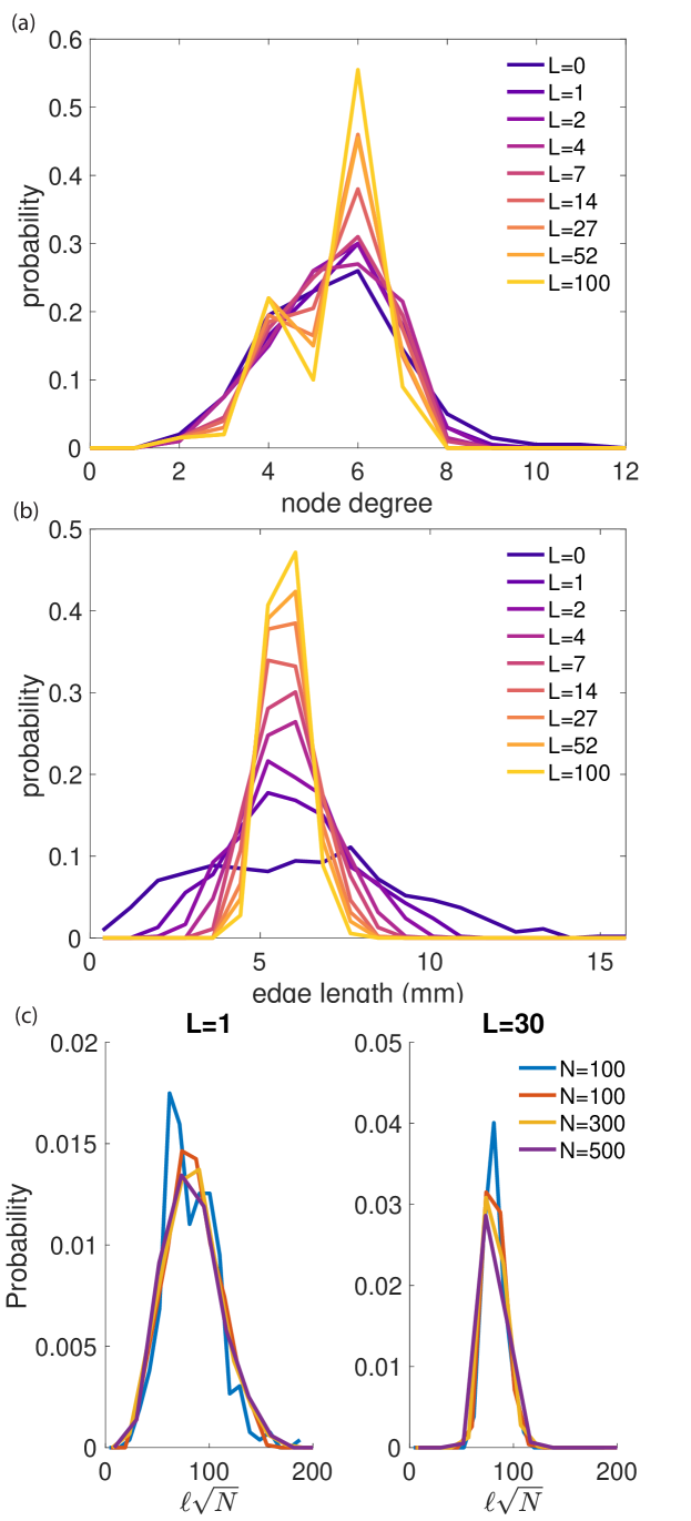
Figure 3: For a single realization of an $N=200$ network subjected to Lloyd’s iterations $L$, its (a) degree distribution $p_{k}$ and (b) probability distribution function $f(\ell)$. (c) Edge-length distributions scaled by $\sqrt{N}$ at Lloyd’s iterations $L=1$ and $L=30$ for networks with increasing number of nodes $N$.

We more directly quantify the disorder of the network through its information entropy $S$. From the histogram plotted in Fig. 3a, we calculate the degree entropy $S_{k}$ as the Shannon entropy

$$S_{k}=-\sum_{k\in D}p_{k}\,\ln p_{k}$$ (2)

where $D$ is the set of all possible degrees collected from the sample. As we will see in Sec. III.2, the effective resistance of the lattice is derived from a network description using edge weights proportional to the conductance $\sigma\propto 1/\ell$. Therefore, we calculate the edge entropy for a network weighted by $c\equiv 1/\ell$; because these values are drawn from a continuous distribution, we use the differential entropy

$$S_{e}=-\int_{\mathbb{R}}g(c)\,\ln g(c)\,dc$$ (3)

where $g(c)$ is the probability density function of the edge-weights $c$, following the method outlined in [23]. The code for performing these calculations is available on GitHub [24].

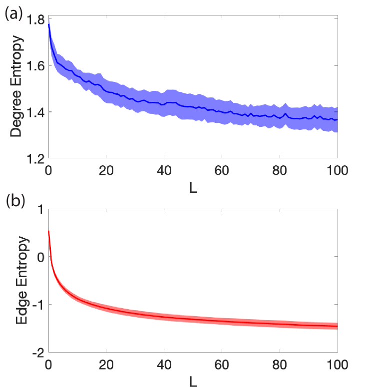
Figure 4: Calculated for an ensemble of 20 realizations of an $N=200$ network, each subjected to Lloyd’s iterations $L$: (a) degree entropy $S_{k}$ calculated using Eq. (2) and (b) edge entropy calculated using Eq. (3). The solid lines are the averages over all 20 realizations, with the shaded region depicting $\pm$ one standard deviation.

These two entropies are plotted in Fig. 4 as a function of the number of iterations of Lloyd’s algorithm. We observe that, as expected, the entropy decreases as the configurations become more ordered at larger $L$. Both $S_{k}$ and $S_{e}$ have their most rapid decrease at low $L$, consistent with both the visual trend noted in Fig. 1 and the changes in edge length distribution shown in Fig. 3b. Note that the differential entropy is not directly comparable with Shannon entropy; for example, the crystalline lattice network with a single value for the edge conductance would have zero Shannon entropy but infinitely negative differential entropy.

III.2 Predicting effective resistance

We compute the total effective resistance diagonally across the network by assigning a resistance to each edge and then creating a system of linear equations using Kirchoff’s laws. We summarize our derivation next to account for variable resistance along each edge, similar to [25]. It is an adaptation of the more common $\mathcal{L}\vec{V}=r\vec{I}$ in the literature (for example, see [26, 27, 12]) where $\mathcal{L}$ is the graph Laplacian, $r$ is a constant resistance for each edge, $\vec{I}$ represents the applied current to each node and $\vec{V}$ is the voltage at each node.

To model the physical samples, we assume each edge is a rectangular rod with a uniform cross-section and length equal to the distance between its endpoints. The resistance of the edge joining nodes $i$ and $j$ is therefore

$$R_{ij}=\frac{\rho\ell_{ij}}{a}$$ (4)

where $\ell_{ij}$ is the length of the edge, $\rho$ is the electrical resistivity of the material, and $a$ the cross-sectional area of the rod. To arrive at a set of equations for the voltage at each node, we begin with Kirchoff’s law that $V=IR$ across each edge, $I_{ij}=(V_{i}-V_{j})/R_{ij}$, with $1/R_{ii}$ defined to be zero. Notice that $I_{ij}=-I_{ji}$ as expected. Applying Kirchoff’s conservation of current at each node $i$, but writing $I_{ij}=(V_{i}-V_{j})/R_{ij}$ yields the following set of $N$ equations

$$\sum_{j=1}^{N}A_{ij}\frac{V_{i}-V_{j}}{R_{ij}}+I_{i}=0\quad\textrm{for }i=1\dots N$$ (5)

where $A_{ij}$ is the adjacency matrix and $I_{i}$ represents the externally applied current to each node. To model the experiment in orientation A(B), we find the NE(NW) clamped node and label it 1 and the SW(SE) clamped node and label it $N$. We then set the externally applied current to be $I_{1}=I_{0},I_{N}=-I_{0}$ and $I_{i}=0$ otherwise.

The system in Eq. (5) can be put into matrix form by first defining a weighted adjacency matrix $\tilde{A}_{ij}=\frac{1}{R_{ij}}$ if nodes $i$ and $j$ are connected by an edge and 0 otherwise, and a weighted graph Laplacian $\tilde{\mathcal{L}}_{ij}=(\delta_{ij}\sum_{j=1}^{N}\tilde{A}_{ij})-\tilde{A}_{ij}$. Then the system in Eq. (5) is

$$\tilde{\mathcal{L}}\vec{V}=\vec{I}$$

The rank of a graph Laplacian is equal to the number of vertices $N$ minus the number of connected components in the graph, meaning for a connected graph like the ones studied here, the rank is always $N-1$. Therefore, only the voltage difference is uniquely defined. Taking $V_{N}=0$ without loss of generality, and solving the first $N-1$ equations we obtain the voltages at each node. The effective resistance of the network is $R_{\textrm{eff}}=V_{1}/I_{0}$ and is independent of the choice of $I_{0}$. Note that the current along each edge is obtained from the voltages using $I_{ij}=(V_{i}-V_{j})/R_{ij}$. The code used for performing these calculations is available on GitHub [28].

Note that the resistivity $\rho$ and the cross-sectional area $a$ simply scale the graph Laplacian and therefore $R_{\textrm{eff}}$. Forming the graph Laplacian matrix $\mathcal{L}_{R}$ using the edge-resistances in Eq. 4 in which length is multiplied by $\rho/a$ is equivalent to forming the Laplacian matrix $\mathcal{L}_{\ell}$ from the edge-resistances given by their lengths $\ell_{ij}$ alone and then dividing by $\rho/a$:

$$\mathcal{L}_{R}=\frac{a}{\rho}\mathcal{L}_{\ell}.$$ (6)

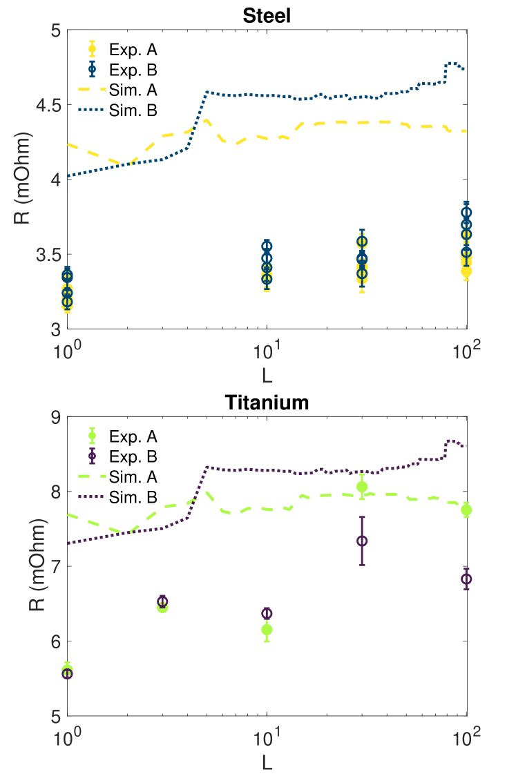
Figure 5: $R_{\textrm{eff}}$ as a function of number of Lloyd’s iterations, $L$, comparing both 4-point measurements (error bars) and predictions from the graph Laplacian (dashed line for orientation A and dotted line for orientation B) for both the steel 17-4PH and the titanium Ti-6Al-4V printed network configurations.

In Fig. 5, we compare these numerically computed $R_{\textrm{eff}}$ values to the values measured on physical samples, described in Sec. II.3. To compute the resistance of each edge according to Eq. (4), we take the cross-sectional area $a=0.03\,\text{cm}^{2}$ for all samples. For 17-4PH steel the resistivity $\rho=98\,\mu\Omega\cdot$cm [29] and for Ti-6Al-4V titanium $\rho=178\,\mu\Omega\cdot$cm [30]. The lateral dimension of the bounding box (2000) corresponds to a printed length of $75$ mm; this ratio is used to convert the computational units for $\ell$ to cm.

From the graph Laplacian method described above, we compute $R_{\textrm{eff}}$ for each iteration of Lloyd’s algorithm applied to the the point cloud realization used to create the printed samples. This result, rescaled to apply to steel vs. titanium using Eq. 6, and calculated for both orientations of the clamped nodes, is shown by the dashed (orientation A) and dotted (orientation B) lines in Fig. 5. With no free parameters, these lines reasonably reproduce the experimentally measured $R_{\textrm{eff}}$ values measured on the printed samples. The error bars on single data points show the standard deviation from 6 repeated measurements on a single sample, and the multiple data points at the same value of $L$ each come from different prints of the same network.

III.3 Current anisotropy

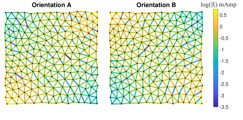
Figure 6: The logarithm of the absolute value of the current flowing through each edge is shown for the $L=10$ network from Fig. 1(b). The current on specific edges depends on both the network topology and the direction of applied voltage.

From the numerical calculation of Sec. III.2, we are able to obtain the current along each edge of the network. An example is shown in Fig. 6, for both orientations of a single $L=10$ realization; the observations we make here hold for all realizations and $L$, whether ordered or disordered. Note that the absolute value of the current is depicted by the color bar since the positive direction is dictated by the order in which the nodes appear in the edge list representation of the matrix, rather than some physical meaning. Colors are assigned to a logarithmic scale to provide visual contrast. We observe that edges more aligned with the line connecting the clamped corners carry more current, as compared to those orthogonal to the direction of applied current. This anisotropy suggests that standard network characterizations such as centrality measures would not capture the global behavior of $R_{\textrm{eff}}$; indeed, we have yet to find a network measure that captures $R_{\textrm{eff}}$.

III.4 Variability among the ensemble of realizations

Figure 7: Calculated $R_{\textrm{eff}}(L)$ for all 20 realizations, measured in both the A and B orientations of the clamped corners. Pink and yellow lines correspond to $N=200$ node networks; cyan and blue lines correspond to $N=500$ node networks.

In Fig. 5, we observed that the numerically-computed value of $R_{\textrm{eff}}$ was in agreement with experimental measurements of the same configuration. However, while this particular realization showed $R_{\textrm{eff}}$ increasing with continued application of Lloyd’s algorithm (progressing towards a more uniform configuration), this trend is inconsistent across the ensemble of initial point clouds taken as the seeds of the 20 independent realizations. Fig. 7 shows the variability $R_{\textrm{eff}}(L)$ for the ensemble of realizations: each solid line follows one point cloud through iterations of Lloyd’s algorithm. A mix of positive and negative slopes, both within a single progression of iterations and between samples, is the prevalent feature. Collectively, there is an observed decrease in the variability in $R_{\textrm{eff}}(L)$ for larger values of $L$. Since Fig. 3b and 4 both quantify a corresponding decrease in the disorder of the network, it appears that this is associated to a decrease in variability of $R_{\textrm{eff}}$.

We also point out that the larger networks ($N=500$ nodes) have lower resistance than the smaller networks ($N=200$) nodes, due to resistors in parallel providing lower effective resistance. The ensemble of larger networks has less variability than the smaller network, at any given value of $L$. A law of large numbers effect could explain this effect: within one network, there are more edges and therefore more paths between the two clamped corners, so it is less likely that the network has a more extreme path leading to larger or smaller resistance. As $L$ increases, both system sizes develop bands of common values of $R_{\textrm{eff}}$. This appears to be due to the partial crystallization of the network being frustrated by the bounding box of the domain.

A common feature of the $R_{\textrm{eff}}(L)$ graphs is that we occasionally observe dramatic changes in $R_{\textrm{eff}}$ due to a single application of Lloyd’s algorithm. In the example shown in Fig. 5, this occurs at $L=5$ and $L=79$, but only for the measurements done in Orientation B, and only for this particular point cloud. Other realizations exhibit similar jumps, as shown in Fig. 7, and these commonly occur in only one of two clamping orientations. To seek an explanation, we quantified the rearrangements within the point cloud using the standard non-affinity measure $D^{2}_{\text{min}}$ [31]. As shown in Fig. 8, we observed that no significant rearrangements occurred at these two $L$ steps. Similarly, there are not any significant rearrangements of the Delaunay triangulation edges. This observation that no significant local change to the configuration is detected, together with the observed sensitivity to the orientation of the applied current, indicates that $R_{\textrm{eff}}$ is arising from the collective effects of the full network. Therefore, the lack of a network summary statistic capturing the changes in $R_{\textrm{eff}}$ is unsurprising.

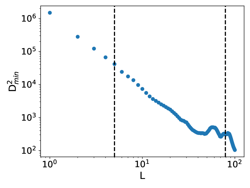
Figure 8: The total $D^{2}_{\textrm{min}}$ for the network as a function of Lloyd’s iteration [31], where the change in position is calculated between subsequent iterations. Vertical dashed lines at $L=5$ and $L=79$ mark the locations of the two jumps in $R_{\textrm{eff}}(L)$ shown in Fig. 5. A movie of the dynamics of the point cloud and of $D^{2}_{\text{min}}$ is available at [17].

IV Discussion and conclusions

We have developed a digital pipeline from algorithmically-created configurations with tunable disorder to printed materials; such materials open a large design space that is suitable for a variety of applications where tunability and low weight are important considerations. This methodology will additionally be applicable to 3D geometries, where disordered metamaterials research is less explored [32, 10] compared with designs based on repeating unit cells. We numerically analyzed our disordered networks as resistor networks to calculate the effective resistance via the graph Laplacian, finding that this method is able to quantitatively capture laboratory measurements of $R_{\textrm{eff}}$ on the printed samples. These direct comparisons demonstrate the feasibility of validating numerical results using a small number of printed samples, setting the stage for future optimization and design in silico rather than iterating through expensive prints.

The freeform nature of additive manufacturing unlocks new algorithm-based design methodologies compared with traditional CAD modeling. This pipeline adds to the toolbox of recently established innovative digital designs such as triply periodic minimized surfaces [33, 34, 35, 36], unit cell lattice structures [37, 4], Voronoi tesselations [38, 39, 40, 41], as well as generative modeling and porous materials [42, 43] to produce non-traditional geometries for applications ranging from heat exchangers to medicine.

For both the single printed sample, and the ensemble of samples studied in silico we observed that common network measures successfully characterize the degree of disorder as a function of the number of iterations of Lloyd’s algorithm, as the point cloud configurations progress from disordered to ordered. Surprisingly, we saw no strong dependence of $R_{\textrm{eff}}$ on the degree of disorder other than a decrease in variability across the ensemble as the degree of disorder decreased. This observation appears at odds with both theoretical [44] and laboratory [45] studies, that photonic band gaps are highly sensitive to the degree and type of hyperuniformity. One possible explanation is that measures of disorder, like the width of the edge distribution or entropy employed here, do not necessarily detect hyperuniformity. Another possible explanation is that not all types of transport are sensitive to the hyperuniformity of a material, which should be explored in future studies. Our inability to find a summary network statistic that could replace the full graph Laplacian (exact solution) suggests that effective resistance is more sensitive to the full network topology than one might think. One challenge to finding such a metric is that we observed a strong anisotropy due to the imposed direction of the driving current, yet topological network measures contain no notion of directionality. Furthermore, jumps in $R_{\textrm{eff}}$ occurred at different steps along the evolution of the configuration, depending on which orientation was chosen for applying the current, and these jumps were not accompanied by large changes in the point cloud configuration as measured by $D_{\min}^{2}$. This work established the feasibility of manufacturing digital designs, creating a pathway to further research on disordered metamaterials, and the development of new characterization metrics.

References

- Mueller et al. [2019] J. Mueller, K. H. Matlack, K. Shea, and C. Daraio, Advanced Theory and Simulations 2, 1900081 (2019).
- Turpin et al. [2014] J. P. Turpin, J. A. Bossard, K. L. Morgan, D. H. Werner, and P. L. Werner, International Journal of Antennas and Propagation 2014, 1 (2014).
- Bauer et al. [2017] J. Bauer, L. R. Meza, T. A. Schaedler, R. Schwaiger, X. Zheng, and L. Valdevit, Advanced Materials 29, 1701850 (2017).
- Askari et al. [2020] M. Askari, D. A. Hutchins, P. J. Thomas, L. Astolfi, R. L. Watson, M. Abdi, M. Ricci, S. Laureti, L. Nie, S. Freear, R. Wildman, C. Tuck, M. Clarke, E. Woods, and A. T. Clare, Additive Manufacturing 36, 101562 (2020).
- Surjadi et al. [2019] J. U. Surjadi, L. Gao, H. Du, X. Li, X. Xiong, N. X. Fang, and Y. Lu, Advanced Engineering Materials 21, 1800864 (2019).
- Ma et al. [2021] W. Ma, Z. Liu, Z. A. Kudyshev, A. Boltasseva, W. Cai, and Y. Liu, Nature Photonics 15, 77 (2021).
- Torquato [2018] S. Torquato, Physics Reports Hyperuniform States of Matter, 745, 1 (2018).
- Siedentop et al. [2024] L. Siedentop, G. Lui, G. Maret, P. M. Chaikin, P. J. Steinhardt, S. Torquato, P. Keim, and M. Florescu, arXiv:2403.08404 10.48550/ARXIV.2403.08404 (2024).
- Zaiser and Zapperi [2023] M. Zaiser and S. Zapperi, Nature Reviews Physics 5, 679 (2023).
- Sniechowski et al. [2015] M. Sniechowski, J. Kaminski, and S. Wronski, VI International Conference on Computational Bioengineering ICCB (2015).
- Lloyd [1982] S. Lloyd, IEEE Transactions on Information Theory 28, 129 (1982), conference Name: IEEE Transactions on Information Theory.
- Newman [2018] M. Newman, Networks (Oxford University Press, 2018).
- Klatt et al. [2019] M. A. Klatt, J. Lovrić, D. Chen, S. C. Kapfer, F. M. Schaller, P. W. A. Schönhöfer, B. S. Gardiner, A.-S. Smith, G. E. Schröder-Turk, and S. Torquato, Nature Communications 10, 811 (2019).
- Hong et al. [2021] S. Hong, M. A. Klatt, G. Schröder-Turk, N. François, and M. Saadatfar, EPJ Web of Conferences 249, 15002 (2021).
- Sames et al. [2016] W. J. Sames, F. A. List, S. Pannala, R. R. Dehoff, and S. S. Babu, International Materials Reviews 61, 315 (2016).
- DebRoy et al. [2018] T. DebRoy, H. L. Wei, J. S. Zuback, T. Mukherjee, J. W. Elmer, J. O. Milewski, A. M. Beese, A. Wilson-Heid, A. De, and W. Zhang, Progress in Materials Science 92, 112 (2018).
- [17] https://youtu.be/f17rt_gqv5e.
- [18] A. T. Becker, lloydsalgorithm, MATLAB Central File Exchange, Accessed on June 2022.
- [19] C. Obrero, github.com/dmref-networks/config_generation.
- Hain et al. [2020] T. M. Hain, M. A. Klatt, and G. E. Schröder-Turk, The Journal of Chemical Physics 153, 234505 (2020).
- Simchi [2006] A. Simchi, Materials Science and Engineering: A 428, 148 (2006).
- Shrestha et al. [2018] R. Shrestha, P. D. Nezhadfar, M. Masoomi, J. Simisiriwong, N. Phan, and N. Shamsaei, Proceedings of the 29th Annual International Solid Freeform Fabrication Symposium – An Additive Manufacturing Conference (2018).
- Vasicek [1976] O. Vasicek, Journal of the Royal Statistical Society. Series B (Methodological) 38, 54 (1976).
- [24] M. Tirfe, github.com/dmref-networks/config_stats.
- Ghosh et al. [2008] A. Ghosh, S. Boyd, and A. Saberi, SIAM Review 50, 37 (2008).
- Klein and Randić [1993] D. J. Klein and M. Randić, Journal of Mathematical Chemistry 12, 81 (1993).
- Newman and Girvan [2004] M. E. J. Newman and M. Girvan, Physical Review E 69, 026113 (2004).
- [28] K. Newhall, github.com/dmref-networks/config_resistance.
- Stashkov et al. [2019] A. Stashkov, E. Schapova, T. Tsar’kova, E. Sazhina, V. Bychenok, A. Fedorov, A. Kaigorodov, and I. Ezhov, Journal of Physics: Conference Series 1389, 012124 (2019).
- Nespoli et al. [2022] A. Nespoli, N. Bennato, E. Villa, and F. Passaretti, Rapid Prototyping Journal 28, 1060 (2022).
- Falk and Langer [1998] M. L. Falk and J. S. Langer, Physical Review E 57, 7192 (1998).
- Wit et al. [2019] A. Wit, S. Wronski, and J. Tarasiuk, Acta Polytechnica CTU Proceedings 25, 89 (2019).
- Dutkowski et al. [2022] K. Dutkowski, M. Kruzel, and K. Rokosz, Energies 15, 7994 (2022).
- Sharma and Hiremath [2022] D. Sharma and S. S. Hiremath, Mechanics of Advanced Materials and Structures 29, 5077 (2022).
- Al-Ketan and Abu Al-Rub [2019] O. Al-Ketan and R. K. Abu Al-Rub, Advanced Engineering Materials 21, 1900524 (2019).
- Chavan et al. [2020] H. Chavan, A. K. Mishra, and A. Kumar, in Advances in Lightweight Materials and Structures, Vol. 8, edited by A. Praveen Kumar, T. Dirgantara, and P. V. Krishna (Springer Singapore, Singapore, 2020) pp. 635–643.
- Van Hooreweder and Kruth [2017] B. Van Hooreweder and J.-P. Kruth, CIRP Annals 66, 221 (2017).
- Bahr et al. [2017] R. A. Bahr, Y. Fang, W. Su, B. Tehrani, V. Palazzi, and M. M. Tentzeris, in 2017 IEEE MTT-S International Microwave Symposium (IMS) (IEEE, Honololu, HI, USA, 2017) pp. 1583–1586.
- Herath et al. [2021] B. Herath, S. Suresh, D. Downing, S. Cometta, R. Tino, N. J. Castro, M. Leary, B. Schmutz, M.-L. Wille, and D. W. Hutmacher, Materials & Design 212, 110224 (2021).
- Hooshmand-Ahoor et al. [2022] Z. Hooshmand-Ahoor, M. Tarantino, and K. Danas, Mechanics of Materials 173, 104432 (2022).
- Martínez et al. [2018] J. Martínez, S. Hornus, H. Song, and S. Lefebvre, ACM Transactions on Graphics 37, 1 (2018).
- Hsu et al. [2022] Y.-C. Hsu, Z. Yang, and M. J. Buehler, APL Materials 10, 041107 (2022).
- Ullah et al. [2020] A. S. Ullah, H. Kiuno, A. Kubo, and D. M. D’Addona, CIRP Annals 69, 113 (2020).
- Klatt et al. [2022] M. A. Klatt, P. J. Steinhardt, and S. Torquato, Proceedings of the National Academy of Sciences 119, e2213633119 (2022).
- Aubry et al. [2020] G. J. Aubry, L. S. Froufe-Pérez, U. Kuhl, O. Legrand, F. Scheffold, and F. Mortessagne, Physical Review Letters 125, 127402 (2020).