Nonlinear Gaussian process tomography with imposed non-negativity constraints on physical quantities for plasma diagnostics.

Abstract

We propose a novel tomographic method, nonlinear Gaussian process tomography (nonlinear GPT) that employs the Laplace approximation to ensure the non-negative physical quantity, such as the emissivity of plasma optical diagnostics. This new method implements a logarithmic Gaussian process (log-GP) to model plasma distribution more naturally, thereby expanding the limitations of standard GPT, which are restricted to linear problems and may yield non-physical negative values. The effectiveness of the proposed log-GP tomography is demonstrated through a case study using the Ring Trap 1 (RT-1) device, where log-GPT outperforms existing methods, standard GPT, and the Minimum Fisher Information (MFI) methods in terms of reconstruction accuracy. The result highlights the effectiveness of nonlinear GPT for imposing physical constraints in applications to an inverse problem.

1 Introduction

Plasma diagnostics play a crucial role in understanding the internal state and structure of plasmas, as well as in controlling fusion plasmas. In-situ diagnostics often provide line-integrated observations, requiring tomographic techniques to obtain cross-sectional distributions for radiation intensity, density, temperature, and velocity.

Inverse problems are generally ill-posed, meaning they often lack a unique solution. Therefore, prior information or constraints must be introduced. Over the years, numerous tomographic methods have been proposed, with Tikhonov regularization being one of the most prominent. The Minimum Fisher Information (MFI) method[1, 2], which uses Fisher information as the Tikhonov regularization term, is widely utilized in plasma diagnostics[3].

Meanwhile, Gaussian Process Tomography (GPT) has emerged as a novel appro ach based on Bayesian inference[4, 5]. GPT models local physical quantities as a Gaussian process, allowing for the estimation of smooth plasma distributions even from sparse and noisy data. This approach has been successfully applied in various contexts, including fitting temperature and density distributions in Thomson scattering[6, 7, 8] and estimating emission intensity distributions in soft X-ray measurements[9, 10]. GPT, as a probabilistic model grounded in Bayesian inference, estimates distributions while quantifying uncertainty through posterior variance. Such frameworks also show promise for the integration of multiple diagnostic datasets[11, 12].

However, a significant limitation of existing GPT methods is their reliance on Gaussian likelihood functions, which restricts the governing equations to linear forms. This limitation can lead to challenges such as non-physical negative emissivity values, reducing reconstruction accuracy and violating physical constraints. To address these challenges, this study introduces a novel approach called Nonlinear Gaussian Process Tomography (nonlinear-GPT) using Laplace approximation. Specifically, this approach employs a logarithmic Gaussian process (log-GP), which enforces non-negativity.

Section 2 describes conventional GP and GPT. Section 3 introduces log-GP and discusses nonlinear-GPT. Section 4 provides a detailed demonstration of the tomography setup, using the RT-1 experiment as a case study. In Section 5, we evaluate the reliability and accuracy of tomography using the nonlinear-GPT method through simulations with phantom data. Finally, Section 6 presents the conclusions of this study.

2 General Methodology of Tomography

2.1 Inverse Problem

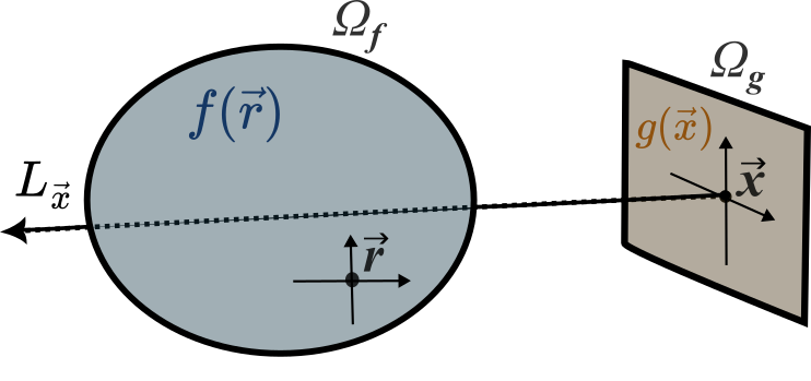
Figure 1: Relation between the local quantity $f$ in the plasma volume $\Omega_{f}$ and the projected observed quantity $g$ in a sensor plane $\Omega_{g}$.

As shown in Fig. 1, the observed quantity $g$ is obtained by integrating the local quantity $f$ along the line of sight, which is represented as:

$$g(\vec{x})=\int_{L_{\vec{x}}}f(\vec{r})\mathrm{d}l+\epsilon,$$ (1)

where, $\vec{x}$ denotes the coordinates in the sensor, $\vec{r}$ denotes the coordinates of the region where plasma behavior occurs, and $L_{\vec{x}}$ represents the path of the line of sight (LOS) specified by $\vec{x}$. By discretizing Eq. 1, the relation between the $N$-dimensional vector of the local variable $\bm{f}$ and the $M$-dimensional observed data $\bm{g}^{\mathrm{obs}}$ is given by adding an observation error term $\bm{\epsilon}$ as:

$$\bm{g}^{\mathrm{obs}}:=\bm{g}(\bm{f})+\bm{\epsilon}=H\cdot\bm{f}+\bm{\epsilon},$$ (2)

where, $H$ is the geometry matrix with dimensions $M\times N$. It can also be represented as $g_{i}=\sum_{j=1}^{N}H_{ij}f_{j}$ for each $i$.

In the general Tikhonov regularization method, tomography is performed by minimizing the following functional:

$$\Lambda[\bm{f}]=(\bm{g}^{\mathrm{obs}}-\bm{g}(\bm{f}))^{\mathrm{T}}\Sigma_{g}^{-1}(\bm{g}^{\mathrm{obs}}-\bm{g}(\bm{f}))+\lambda\Lambda_{\mathrm{r}}[\bm{f}],$$ (3)

where, $\Sigma_{g}$ is the covariance matrix of the error term, $\Lambda_{\mathrm{r}}[\bm{f}]$ is the regularization term, $\lambda$ is a regularization parameter, and the superscript ^T denotes the transpose of the vector or matrix. The MFI method, which uses Fisher information as a regularization term, is often employed in plasma diagnostics. Formally, the regularization term is expressed as:

$$\Lambda^{\mathrm{MFI}}_{\mathrm{r}}[\bm{f}]=\sum_{i=1}^{N}\frac{1}{f_{i}}(\bm{\nabla}f)_{i}\cdot(\bm{\nabla}f)_{i}.$$ (4)

MFI achieves a non-negative solution, since the smaller the amplitude, the stronger the smoothness constraint. However, it requires iterative computation because its regularization term for $\bm{f}$ is nonlinear.

2.2 Gaussian Process

When a function $f$ is modeled as a Gaussian process, we denote this as $f\sim\mathcal{GP}(\mu,k)$, where $\mu$ is the mean function and $k$ is the kernel (or covariance) function. For any finite set of input points $\bm{r}:=\{r_{i}\}_{i=1}^{N}$, the corresponding function values $\bm{f}=f(\bm{r})$ follow a multivariate normal distribution, denoted as $\bm{f}\sim\mathcal{N}(\mathbf{\mu},K)$. Here, $\mathbf{\mu}$ is the mean vector with components $\mu_{i}=\mu(r_{i})$, and $K$ is the covariance matrix with entries $K_{ij}=k(r_{i},r_{j})$. The probability density function(PDF) of the $N$-variate normal distribution is given by:

$$p(\bm{f})=\mathcal{N}(\bm{f}\mid\bm{\mu},\Sigma):=(2\pi)^{-N/2}|\Sigma|^{-1/2}\exp\left(-\frac{1}{2}(\bm{f}-\bm{\mu})^{\mathrm{T}}\Sigma^{-1}(\bm{f}-\bm{\mu})\right).$$ (5)

The squared exponential (SE) kernel is the de facto standard kernel in GP and has the following form:

$$k_{\mathrm{SE}}(r,r^{\prime})=\sigma_{f}^{2}\exp\left(-\frac{1}{2}\frac{(r-r^{\prime})^{2}}{\ell^{2}}\right),$$

where, $\ell$ is the length scale, which controls the smoothness of $f$ and defines its spatial scale, and $\sigma_{f}$ is the output scale that controls its amplitude. When considering inhomogeneous length scales and multidimensional input spaces $\vec{r}$, a generalized SE kernel called the Gibbs kernel [13, 5] has the form:

$$k(\vec{r},\vec{r}^{\prime})=\sigma_{f}^{2}\frac{|\Sigma_{\ell\ell}|^{\frac{1}{4}}|\Sigma_{\ell^{\prime}\ell^{\prime}}|^{\frac{1}{4}}}{\left|\frac{1}{2}\Sigma_{\ell\ell}+\frac{1}{2}\Sigma_{\ell^{\prime}\ell^{\prime}}\right|^{\frac{1}{2}}}\exp\left(-(\vec{r}-\vec{r}^{\prime})^{\mathrm{T}}\left(\Sigma_{\ell\ell}+\Sigma_{\ell^{\prime}\ell^{\prime}}\right)^{-1}(\vec{r}-\vec{r}^{\prime})\right).$$ (6)

Here, $\Sigma_{\ell\ell}$ is a positive semi-definite matrix that generalizes the distance metric in the space. Under the assumption of an isotropic length scale, it becomes a scalar multiple of the identity matrix:

$$\Sigma_{\ell\ell}=\ell^{2}(\vec{r})I=\left[\begin{array}[]{cc}\ell^{2}(\vec{r})&0\\ 0&\ell^{2}(\vec{r})\end{array}\right],$$ (9)

where, $I$ is the identity matrix and $\ell(\vec{r})$ is the position-dependent length scale function.

2.3 Gaussian process tomography

In GPT[4, 5], the problem described by Eq. 2 is formulated with the following assumptions:

$$\bm{\epsilon}\sim\mathcal{N}(\bm{0},\Sigma_{g}),\quad \bm{f}\sim\mathcal{N}(\bm{\mu}_{f}^{\mathrm{pri}},K_{f}).$$

This formulation enables the posterior distribution, $p(\bm{f}\mid\bm{g}^{\mathrm{obs}})$, to be derived using Bayes’ rule. The posterior distribution is denoted as $\mathcal{N}(\bm{f}\mid\bm{\mu}_{f}^{\mathrm{post}},\Sigma_{f}^{\mathrm{post}})$. The known formula for GPT is expressed as follows:

$$\bm{\mu}_{f}^{\mathrm{post}}=\bm{\mu}_{f}^{\mathrm{pri}}+(H^{\mathrm{T}}\Sigma_{g}^{-1}H+K_{f}^{-1})^{-1}H^{\mathrm{T}} \Sigma_{g}^{-1}(\bm{g}^{\mathrm{obs}}-H\bm{\mu}_{f}^{\mathrm{pri}})$$ (10)

$$\Sigma_{f}^{\mathrm{post}}=(H^{\mathrm{T}}\Sigma_{g}^{-1}H+K_{f}^{-1})^{-1}.$$

In GPT, the term $\bm{f}^{\mathrm{T}}K_{f}^{-1}\bm{f}$ plays the role of the regularization term $\Lambda_{r}[\bm{f}]$ in the Tikhonov method, as expressed in Eq. 3. This term acts as a prior on the smoothness of $\bm{f}$, enforcing the expected spatial correlation defined by the kernel $K_{f}$. The advantage of GPT is that the kernel matrix $K_{f}$ allows it to represent a wide range of function shapes and correlations, which is challenging for conventional regularization methods. Additionally, GPT provides a probabilistic framework where the posterior variance matrix $\Sigma_{f}^{\mathrm{post}}$ offers a quantification of the uncertainty in the reconstructed solution, enabling error prediction and confidence assessment.

3 Nonlinear Gaussian process tomography

3.1 Log-gaussian process

The challenge with standard GPT is the limitation that it can only solve linear problems. For example, the accuracy of tomography could be improved if it were possible to impose a non-negativity constraint on physical quantities such as plasma spectra or X-ray emissivity; methods such as MFI and Maximum Entropy[14] can impose this constraint. However, standard GPT does not incorporate such physical constraints.

To address this problem, we introduce a latent variable $\hat{f}$, such that $f=\exp(\hat{f})$. Instead of directly modeling the physical quantity $f$ as a Gaussian process, we model $\hat{f}$ as a Gaussian process:

$$f=\exp{\hat{f}},\quad\hat{f}\sim\mathcal{GP}$$ (11)

In this case, $f$ is referred to as a ”log-Gaussian process” (log-GP) extending the log-normal distribution to the function space and is denoted as $f\sim\mathrm{log}\mathcal{GP}$. This formulation often appears as an intermediate variable to enforce non-negativity, for example, in Gaussian process classification [15] and log-Gaussian Cox processes [16].

The log-GP has the following key properties:

• Non-negativity: The variable $f$ always takes positive values, which can be formally expressed as:

  $$\mathrm{supp}[\;p(f)\;]=(0,+\infty),\quad\mathrm{where}\;f\sim\mathrm{log}\mathcal{GP}.$$ (12)

  Here, $\mathrm{supp}[\cdot]$ denotes the support of a function, and $p(f)$ represents PDF of the log-GP. The mean function $\mu$ primarily determines the scale of $f$, while the output scale $\sigma_{f}$ controls its dynamic range.

• Closure under multiplication: The log-GP is closed under multiplication. In contrast to Gaussian processes, which are closed under addition and subtraction, the product or quotient of two log-GPs yields another log-GP:

  $$f_{1},f_{2}\sim\log\mathcal{GP}\Rightarrow f_{1}\cdot f_{2}\sim\log\mathcal{GP}.$$ (13)

  This property is particularly useful in plasma physics, for example, when estimating plasma pressure from density and temperature ($p=nT$) or calculating the ratio of spectral intensities ($I_{A}/I_{B}$).

• Gradient length: When $\hat{f}=\log{f}$ has an SE kernel, the variance of $\frac{1}{f}\frac{df}{dx}$ is the inverse of the length scale $\ell(x)^{2}$, which is described generally as:

  $$\mathrm{Var}\left(\frac{\bm{\nabla}f}{f}\right)=\mathrm{Var}\left(\bm{\nabla}\hat{f}\right)=\Sigma_{\ell\ell}^{-1},$$ (14)

  where, $\mathrm{Var}(\cdot)$ denotes the variance of a variable. In the context of transport analysis[17], $f/\nabla f$ is defined as the ”gradient length,” which implies that the standard deviation of the gradient length corresponds to the length scale in log-GP with SE kernels.

• Mean and mode: The mean value of a log-GP does not equal $\exp(\mu)$. Similar to a log-normal distribution, the mean is $\exp(\mu+\frac{1}{2}\sigma_{f}^{2})$, while the mode of the log-GP remains $\exp(\mu)$.

• Connection to stochastic processes: The log-GP is associated with geometric Brownian motion and can be obtained as a solution to a stochastic differential equation when spatial directions are correlated based on a kernel function.

From the above, log-GP is often more suitable than existing Gaussian processes for estimating physical quantities expressed on a logarithmic scale, such as density, energy, temperature, and radiance. However, even for such physical quantities, the advantage of log-GP diminishes when the relative change is sufficiently small compared to the absolute amount ($\Delta f\ll f$). Furthermore, log-GP cannot be applied to physical quantities taking both positive and negative values, such as velocity.

3.2 Log-Gaussian Process Tomography

When the local physical quantity is modeled as a log-GP, the relation between the observed data and the local variable can be expressed as:

$$\bm{g}^{\mathrm{obs}}:=\bm{g}{(\hat{\bm{f}})}+\bm{\epsilon}=H\cdot\exp{\hat{\bm{f}}}+\bm{\epsilon}.$$

Under the assumptions that $\bm{\epsilon}\sim\mathcal{N}(\bm{0},\Sigma_{g})$ and $\bm{\hat{f}}\sim\mathcal{N}(\bm{\mu}^{\mathrm{pri}},K_{f})$, the posterior probability of the variable $\hat{\bm{f}}$ is formulated as:

$$\underbrace{\log{p(\hat{\bm{f}}|\bm{g}^{\mathrm{obs}})}}_{\mathrm{posterior}} = \underbrace{-\frac{1}{2}(H\cdot\exp{\hat{\bm{f}}}-\bm{g}^{\mathrm{obs}})^{\mathrm{T}}\Sigma_{g}^{-1}(H\cdot\exp{\hat{\bm{f}}}-\bm{g}^{\mathrm{obs}})}_{\mathrm{likelihood}}$$

$$\underbrace{-\frac{1}{2}(\bm{\hat{f}}-\bm{\mu}^{\mathrm{pri}})^{\mathrm{T}}K_{f}^{-1}(\bm{\hat{f}}-\bm{\mu}^{\mathrm{pri}})}_{\mathrm{prior}}+\,C,$$

where, $C$ is a constant term that does not depend on $\hat{\bm{f}}$.

In the non-linear case, the likelihood function $p(\bm{g}^{\mathrm{obs}}\mid\bm{f})$ follows a non-Gaussian distribution, making an analytical solution for the posterior probability intractable. As an alternative to obtaining an exact solution, sampling the posterior probability using Markov chain Monte Carlo methods has been proposed[18]. However, due to the ”curse of dimensionality,” such methods often require significant computation time, especially in cases where $N\gg 1000$. In these situations, an approximate solution can be derived by employing a quasi-probability distribution, such as $q(\bm{f}):=\mathcal{N}(\bm{f};\tilde{\bm{\mu}},\tilde{\Sigma})$, approximating the true posterior probability $p(\hat{\bm{f}}\mid\bm{g}^{\mathrm{obs}})$ as:

$$p(\hat{\bm{f}}\mid\bm{g}^{\mathrm{obs}})\simeq q(\hat{\bm{f}})=\mathcal{N}(\hat{\bm{f}}\mid\tilde{\bm{\mu}},\tilde{\Sigma}),$$ (15)

with $\tilde{\bm{\mu}}$ and $\tilde{\Sigma}$ estimated accordingly. Various methods have been proposed for determining how to approximate the posterior [19], with known approaches including Laplace approximation [20], expectation propagation [21], and variational inference based on the Kullback-Leibler divergence [22, 23].

3.3 Laplace Approximation Method

The log-GP developed here employs the Laplace approximation method, which offers higher computational efficiency compared to other methods, although it is inferior in approximation accuracy. We denote the estimated mean and covariance in the Laplace approximation as $\tilde{\mu}_{\mathrm{LA}}$ and $\tilde{\Sigma}_{\mathrm{LA}}$, respectively.

This method involves performing a Taylor series of the log posterior probability $\log{p(\bm{f}|\bm{g}^{\mathrm{obs}})}$ up to the quadratic term around the maximum a posteriori (MAP) estimate $\tilde{\bm{f}}_{\mathrm{MAP}}$, and matching the coefficients with the mean and variance of $q(\bm{f})$.

The details of the Laplace approximation are as follows. We define a function $\Psi(\bm{f})$ as:

$$\Psi(\bm{f}):=\log{p(\bm{f}|\bm{g}^{\mathrm{obs}})}+C.$$ (16)

The Taylor series of $\Psi(\bm{f})$ around a point $\bm{f}=\bm{b}$ yields:

$$\Psi(\bm{f})=\Psi(\bm{b})+(\bm{f}-\bm{b})^{\mathrm{T}}\bm{\nabla}\Psi_{(\bm{b})}+(\bm{f}-\bm{b})^{\mathrm{T}}\nabla^{2}\Psi_{(\bm{b})}(\bm{f}-\bm{b})+\cdots+C,$$

where, $\bm{\nabla}\Psi_{(\bm{b})}$ and $\nabla^{2}\Psi_{(\bm{b})}$ are defined as follows:

$$\bm{\nabla}\Psi_{(\bm{b})}:=\left.\frac{\partial\Psi(\bm{f})}{\partial\bm{f}}\right|_{\bm{f}=\bm{b}},\quad\nabla^{2}\Psi_{(\bm{b})}:=\left.\frac{\partial^{2}\Psi(\bm{f})}{\partial\bm{f}\partial\bm{f}}\right|_{\bm{f}=\bm{b}}.$$

By substituting $\bm{b}=\bm{f}_{\mathrm{MAP}}$ and using $\bm{\nabla}\Psi{(\tilde{\bm{f}}_{\mathrm{MAP}})}=\bm{0}$, we obtain:

$$\Psi(\bm{f})\simeq(\bm{f}-\bm{f}_{\mathrm{MAP}})^{\mathrm{T}}\nabla^{2}\Psi_{(\bm{f}_{\mathrm{MAP}})}(\bm{f}-\bm{f}_{\mathrm{MAP}})+C.$$ (17)

By equating Eq. 17 with the exponent of $q(\bm{f})=\mathcal{N}(\bm{f}\mid\tilde{\bm{\mu}}^{\mathrm{LA}},\tilde{\Sigma}^{\mathrm{LA}})$, the following correspondences are derived:

$$\tilde{\bm{\mu}}^{\mathrm{LA}}=\bm{f}_{\mathrm{MAP}},\quad\tilde{\Sigma}^{\mathrm{LA}}=-\nabla^{2}\Psi_{(\bm{f}_{\mathrm{MAP}})}^{-1}.$$ (18)

3.4 Solving with Newton-Raphson

To find $\bm{f}_{\mathrm{MAP}}$, one can solve the optimization problem of minimizing $\Psi$. For this problem, the most efficient approach is to use the Newton-Raphson method[15], which is expressed as:

$$\tilde{\bm{f}}^{\mathrm{old}}\rightarrow\tilde{\bm{f}}^{\mathrm{new}};\quad\tilde{\bm{f}}^{\mathrm{new}}=\tilde{\bm{f}}^{\mathrm{old}}-\nabla^{2}\Psi_{(\tilde{\bm{f}}^{\mathrm{old}})}^{-1}\cdot\bm{\nabla}\Psi_{(\tilde{\bm{f}}^{\mathrm{old}})}.$$ (19)

The update of $\tilde{\bm{f}}$ is iteratively computed until $\bm{\nabla}\Psi_{(\tilde{\bm{f}})}\simeq\bm{0}$ is satisfied. When adopting the Newton-Raphson method in Eq. 19, both the gradient of the posterior $\bm{\nabla}\Psi_{(\tilde{\bm{f}})}$ and the inverse of the Hessian matrix $\nabla^{2}\Psi_{(\tilde{\bm{f}})}^{-1}$ need to be calculated in each iteration. This inverse matrix is also used to determine the estimated posterior variance $\tilde{\Sigma}_{\mathrm{LA}}$ after the iterations converge.

In the case of log-GPT, $\Psi(\tilde{\bm{f}})$ is expressed as:

$$\Psi(\tilde{\bm{f}})=-\frac{1}{2}(\bm{g}{(\tilde{\bm{f}})}-\bm{g}^{\mathrm{obs}})^{\mathrm{T}}\Sigma_{g}^{-1}(\bm{g}{(\tilde{\bm{f}})}-\bm{g}^{\mathrm{obs}})-\frac{1}{2}(\tilde{\bm{f}}-\bm{\mu}^{\mathrm{pri}})^{\mathrm{T}}K^{-1}(\tilde{\bm{f}}-\bm{\mu}^{\mathrm{pri}}).$$

Consequently, $\bm{\nabla}\Psi_{(\tilde{\bm{f}})}$ and $\nabla^{2}\Psi_{(\tilde{\bm{f}})}$ can be derived for each $i$ and $j$ using matrix calculus as follows:

$$\{\bm{\nabla}\Psi_{(\tilde{\bm{f}})}\}_{i} = \left.{\frac{\partial\Psi(\hat{\bm{f}})}{\partial\hat{f}_{i}}}\right|_{\hat{\bm{f}}=\tilde{\bm{f}}}$$ (21)

$$= \{H^{\mathrm{T}}\Sigma_{g}^{-1}\cdot(\bm{g}{(\tilde{\bm{f}})}-\bm{g}^{\mathrm{obs}})\}_{i}\,\exp{\tilde{f}_{i}}$$

$$- \{K^{-1}\cdot(\tilde{\bm{f}}-\bm{\mu}^{\mathrm{pri}})\}_{i},$$

$$\{\nabla^{2}\Psi_{(\tilde{\bm{f}})}\}_{ij} = \left.\frac{\partial^{2}\Psi(\hat{\bm{f}})}{\partial\hat{f}_{i}\partial\hat{f}_{j}}\right|_{\hat{\bm{f}}=\tilde{\bm{f}}}$$ (22)

$$= \{H^{\mathrm{T}}\Sigma_{g}^{-1}H\}_{ij}\,\exp{\tilde{f}_{i}}\,\exp{\tilde{f}_{j}}$$

$$- \delta_{ij}\{H^{\mathrm{T}}\Sigma_{g}^{-1}\cdot(\bm{g}{(\tilde{\bm{f}})}-\bm{g}^{\mathrm{obs}})\}_{i}\exp{\tilde{f}_{i}}$$

$$- \{K^{-1}\}_{ij},$$

where $\delta_{ij}$ is the Kronecker delta. The following pseudocode is provided:

Algorithm 1 Newton-Raphson Laplace Approximation

0:  $\bm{f}^{\mathrm{post}}\sim\mathcal{N}(\tilde{\bm{\mu}}^{\mathrm{LA}},\tilde{\Sigma}^{\mathrm{LA}})$

1:  $\tilde{\bm{f}}\leftarrow\tilde{\bm{f}}^{\mathrm{\,init}}$

2:  while $\|\bm{\nabla}\Psi\|\neq\bm{0}$ do

3:     $\bm{\nabla}\Psi\leftarrow\bm{\nabla}\Psi(\tilde{\bm{f}})\quad$ # Eq. 21

4:     $\nabla^{2}\Psi\leftarrow\nabla^{2}\Psi(\tilde{\bm{f}})\quad$ # Eq. 22

5:     $\bm{\Delta}\tilde{f}\leftarrow{(\nabla^{2}\Psi)}^{-1}\cdot\bm{\nabla}\Psi$

6:     $\tilde{\bm{f}}\leftarrow\tilde{\bm{f}}+\alpha\bm{\Delta}\tilde{f};\quad 0<\alpha\leq 1$

7:  end while

8:  $\tilde{\bm{\mu}}^{\mathrm{LA}}\leftarrow\tilde{\bm{f}},\quad\tilde{\Sigma}^{\mathrm{LA}}\leftarrow-({\nabla^{2}}\Psi)^{-1}$

In Algorithm 1, $\alpha$ is the step size for the line search. Choosing an $\alpha$ that minimizes $\|\bm{\nabla}\Psi(\tilde{\bm{f}}+\alpha\bm{\Delta}\tilde{f})\|$ accelerates convergence. The speed of convergence also depends on the initial value of $\tilde{\bm{f}}$; empirically, it is often faster to assign a scalar value slightly larger than $\mu$. Additionally, since exponential calculations are involved during iterations, there is a risk of arithmetic overflow. One way to mitigate this is by setting a maximum value for the absolute change in $\bm{\Delta}\tilde{f}$.

3.5 Optimization of hyperparameters

In GPT, the mean and covariance matrix of the prior $\mathcal{N}(\bm{\mu}^{\mathrm{pri}},K_{f})$ for the local variable $\bm{f}$ and the covariance matrix $\Sigma_{g}$ for the error $\bm{\epsilon}$ must be specified in advance. These parameters, $\bm{\mu}^{\mathrm{pri}}$, $K_{f}$, and $\Sigma_{g}$, collectively referred to as hyperparameters and represented by the vector $\bm{\theta}$, are typically optimized by maximizing the marginal likelihood (or evidence), defined by:

$$\mathcal{L}(\bm{\theta}):=p(\bm{g}^{\mathrm{obs}};\bm{\theta})=\int p(\bm{g}^{\mathrm{obs}},\bm{f};\bm{\theta})\mathrm{d}\bm{f}.$$ (23)

For nonlinear-GPT,it is nearly impossible to obtain Eq. 23 analytically. However, under the Laplace approximation, an approximate solution can be derived using Taylor series:

$$\log\mathcal{L}(\bm{\theta})\simeq\log\Psi(\tilde{\mu}_{\mathrm{LA}})+\frac{1}{2}\log|\tilde{\Sigma}_{\mathrm{LA}}|.$$

The evidence for log-GPT model is calculated as:

$$2\log\mathcal{L}(\bm{\theta}) = -(\bm{g}{(\tilde{\bm{\mu}}^{\mathrm{LA}})}-\bm{g}^{\mathrm{obs}})^{\mathrm{T}}\Sigma_{g}^{-1}(\bm{g}{(\tilde{\bm{\mu}}^{\mathrm{LA}})}-\bm{g}^{\mathrm{obs}})$$ (24)

$$-(\bm{\tilde{\mu}}^{\mathrm{LA}}-\bm{\mu}^{\mathrm{pri}})^{\mathrm{T}}K_{f}^{-1}(\bm{\tilde{\mu}}^{\mathrm{LA}}-\bm{\mu}^{\mathrm{pri}})$$

$$-\log|K|-\log|\Sigma_{g}|+\log|\tilde{\Sigma}_{\mathrm{LA}}|$$

The optimal hyperparameters can be obtained by maximizing the log-evidence. However, directly optimizing all parameters (e.g., $n$ for $\bm{\mu}^{\mathrm{pri}}$, $(n^{2}+n)/2$ for $K$, $(m^{2}+m)/2$ for $\Sigma_{g}$) is computationally intensive. Therefore, a simplified approach normalizes the length scale (Eq. 9) and error covariance:

$$\ell(\vec{r})=\hat{\ell}_{s}\ell^{\prime}(\vec{r}),\quad\Sigma_{g}=\sigma^{2}_{s}\hat{\sigma}^{2}_{g}(\vec{x}),$$ (25)

where, $\hat{\ell}_{s}$ and $\sigma_{s}$ are scale parameters, and $\ell^{\prime}(\vec{r})$ and $\hat{\sigma}_{g}(\vec{x})$ represent spatial dependencies, which can be estimated empirically.

Studies that model Gaussian processes with heteroscedastic variance and optimize inhomogeneous kernels are attractive because they extend the range of applications to real tomography. However, applying these methods to large-scale nonlinear Gaussian Process Tomography remains a challenge for future work.

4 Tomography for optical diagnostic at the RT-1 device

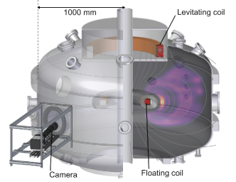
Figure 2: The magnetospheric plasma device RT-1 and camera system. The camera is set to view a poloidal cross-section of RT-1 torus plasmas and to diagnose an emission from helium ions[24]. The emissivity profile from the plasma is overlaid on the magnetic field lines.

In this section, we discuss the implementation of log-GPT. To perform tomography, several factors must be determined: the instrument structure, the instrument’s field of view, boundary conditions, the likelihood function, and the geometry matrix $H$. We focus on spectroscopic measurements in the RT-1 device at the University of Tokyo, which is capable of generating laboratory magnetospheric plasmas (Fig. 2). The RT-1 device is composed of a superconducting coil in a vacuum vessel. The coil is magnetically levitated by an external normal-conducting coil to generate a dipole magnetic field in which the plasma is confined[25]. Using RT-1, We have generated plasmas and observed physical phenomena unique to dipole plasmas, such as plasma pressures exceeding the magnetic field pressure $(\beta>1)$[26], Van Allen belt-like band structures with high-energy electrons[27], toroidal flows accelerated by ion heating[28], and chorus emissions[29]. Due to the absence of magnetic ripple, the RT-1 plasma is purely axisymmetric, which allows for the reconstruction of toroidal cross-sections even from a single image[30].

4.1 Length scale distribution

To apply the Gibbs kernel given by Eq 6 in log-GPT, we need to specify the length scale distribution $\ell(\vec{r})=\hat{\ell}_{S}\ell^{\prime}(\vec{r})$. In the RT-1 device, $\ell^{\prime}(\vec{r})$, as shown in Fig. 3, is in the range from 1 cm to 6 cm, which were given empirically from the density and temperature profiles of the RT-1 plasma; $\ell^{\prime}(\vec{r})$ inside the plasma confined area is gradually scaled and connected to the outside of the last closed flux surface (LCFS) and the surface of the superconducting coil case where the plasma lost. The length scale factor $\hat{\ell}_{S}$ is optimized by maximizing the evidence given by Eq. 24. The use of this inhomogeneous length scale contributes to improved reconstruction accuracy and reduces the size of the vector $\bm{f}$, as described in the following subsection.

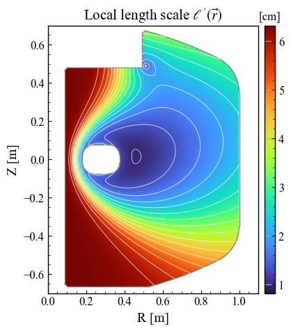
Figure 3: The referenced length scale distribution $\ell^{\prime}(\vec{r})$ on the cross-section of RT-1, corresponds to in Eq. 25

4.2 Inducing points

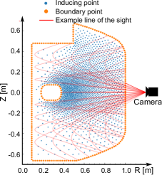
Figure 4: The distribution of inducing points $\vec{r}^{\mathrm{\,idc}}$ (the blue points), boundary points $\vec{r}^{\mathrm{\,bd}}$ (the orange points), and rays for the LOS (the red lines) that start from the camera. These rays are projected onto the poloidal cross-section of the RT-1 device. The number of inducing points is 2041, and the number of boundary points is 229 in the setup. The number of rays is reduced for simplicity.

Functions of physical quantities that follow a GP or log-GP are discretized for numerical computation, which requires defining a set of input spatial points in $\Omega_{f}$, represented by $\vec{\bm{r}}$. Typically, $\vec{\bm{r}}$ is arranged on a grid, simplifying the computation of gradients as seen in Eq. 4 and other operations. However, in this study, we employed a scattered distribution that is not constrained by a grid structure, as shown in Fig. 4. In the context of Sparse Gaussian Process Regression[31], inducing points are defined as $\bm{f}^{\mathrm{idc}}=f(\vec{\bm{r}}^{\mathrm{\,idc}})$, where $\vec{\bm{r}}^{\mathrm{\,idc}}$ is a set of inducing input points. The inducing points are placed so that the distance between adjacent points is approximately equal to the referenced length scale $\ell^{\prime}(\vec{r})$. This is based on the principle that the minimum interval of input point, $\Delta x$, required to maintain the accuracy of interpolation in the SE kernel is nearly equal to the length scale $\ell$. In other words, the distribution of the inducing points determines the lower limit of the length scale. Thus, while searching for the optimal hyperparameters, the length scale factor $\ell_{S}$ (defined in 25) must be greater than one. Such usage of arbitrary inducing points is expected to significantly reduce the size of the local variable $\bm{f}$. This advantage is significant for nonlinear GPT, as the iterative process often requires substantial computational time.

4.3 Geometry Matrix

The variable $\bm{f}^{\mathrm{idc}}$ induces an approximate value at an arbitrary point through the inner product with the weighting functions, as indicated by the equation: $\tilde{f}(\vec{r})\simeq\hat{\bm{w}}(\vec{r})^{\mathrm{T}}\cdot\bm{f}^{\mathrm{idc}}$. Substituting this variable into Eq. 1 yields the following relationship between $\bm{g}$ and $\bm{f}^{\mathrm{idc}}$:

$$g(\vec{x}_{i})\simeq\int_{L_{i}}\sum_{j=1}^{N}\hat{\omega}_{j}(\vec{r}){f}^{\mathrm{idc}}_{j}\mathrm{d}l=\sum_{j=1}^{N}\left(\int_{L_{i}}\hat{\omega}_{j}(\vec{r})\mathrm{d}l\right){f}^{\mathrm{idc}}_{j}.$$ (26)

Considering the equation $\bm{g}=H\cdot\bm{f}^{\mathrm{idc}}$, the matrix $H$ is derived as:

$$H_{ij}\simeq\int_{L_{i}}\hat{\omega}_{j}(\vec{r})\mathrm{d}l,$$ (27)

where, $i$ denotes the index of the LOS corresponding to the pixel on the sensor plane, and $j$ denotes the index of the inducing points. There are several approaches to define the weighting function. For instance, the kernel interpolation method, which is expressed as $\hat{{\omega}}_{j}(\vec{r})=\sum_{i}^{N}k(\vec{r},\vec{r}^{\mathrm{\,idc}}_{i})\{K^{\mathrm{idc}}\}^{-1}_{ij}$, might be consistent in terms of the function space[32]. Alternatively, when the dimension of the observed data $M$ is very large, as in the case of imaging measurements such as our research, we employed the ratio of the kernel functions as the weighting function to ensure the sparsity of the matrix. The weighting functions are defined as:

$$\hat{\omega}_{j}(\vec{r})=\frac{k(\vec{r},\vec{r}^{\mathrm{\,idc}}_{j})}{\sum_{k=1}^{N}k(\vec{r},\vec{r}^{\mathrm{\,idc}}_{k})},$$ (28)

where, $k(\vec{r},\vec{r})$ is the generalized Gibbs kernel function defined in Eq. 6, and $\ell(\vec{r})$ is set to be the same distribution as the length scale in Fig. 3. The function $k(\vec{r},\vec{r}^{\mathrm{\,idc}})$ rapidly approaches zero when the distance between $\vec{r}^{\mathrm{\,idc}}$ and $\vec{r}$ exceeds several times of ${\ell}^{\prime}(\vec{r})$. Consequently, the weighting function $\hat{\omega}_{j}(\vec{r})$ becomes nearly zero, which results in sparsity in the geometry matrix.

4.4 Boundary Conditions

The boundary conditions are imposed such that the value of the local quantities is zero at the container wall. One way to incorporate boundary conditions within Bayesian estimation is to construct conditional probabilities based on prior probabilities.

In this approach, the joint probability distribution of $f(\vec{\bm{r}}^{\mathrm{\,idc}})$ and $f(\vec{\bm{r}}^{\mathrm{\,bd}})$ is considered as:

$$\left[\begin{array}[]{c}\bm{f}^{\mathrm{idc}}\\ \bm{f}^{\mathrm{bd}}\end{array}\right]\sim\mathcal{N}\left(\left[\begin{array}[]{c}\bm{\mu}^{\mathrm{idc}}\\ \bm{\mu}^{\mathrm{bd}}\end{array}\right],\left[\begin{array}[]{cc}K^{\mathrm{idc}}&K^{\mathrm{idc,bd}}\\ K^{\mathrm{bd,idc}}&K^{\mathrm{bd}}+\sigma^{2}I\end{array}\right]\right),$$

and then the conditional probability is calculated given $f(\vec{\bm{r}}^{\mathrm{\,bd}})\sim\mathcal{N}(\bm{y}^{\mathrm{\,bd}},\sigma^{2}I)$. Using the well-known formula for the conditional probability of a multivariate normal distribution, the mean and covariance of $\bm{f}^{\mathrm{idc}}$ are updated as:

$$\bm{\mu}^{\mathrm{idc}\mid\mathrm{bd}} = \bm{\mu}^{\mathrm{idc}}+K^{\mathrm{idc,bd}}(K^{\mathrm{bd}}+\sigma^{2}I)^{-1}(\bm{y}^{\mathrm{bd}}-\bm{\mu}^{\mathrm{bd}}),$$

$$K^{\mathrm{idc}\mid\mathrm{bd}} = K^{\mathrm{idc}}-K^{\mathrm{idc,bd}}(K^{\mathrm{bd}}+\sigma^{2}I)^{-1}K^{\mathrm{bd,idc}}.$$ (30)

Here, $K^{\mathrm{idc,bd}}$ and $K^{\mathrm{bd,idc}}$ are the covariance matrices between the interior points (inducing points) and the boundary points, defined as $K^{\mathrm{idc,bd}}_{ij}=k(\vec{r}^{\mathrm{\,idc}}_{i},\vec{r}^{\mathrm{\,bd}}_{j})$ and $K^{\mathrm{bd,idc}}={(K^{\mathrm{idc,bd}}})^{\mathrm{T}}$. $K^{\mathrm{bd}}$ and $K^{\mathrm{idc}}$ are the covariance matrices within the boundary and interior points, respectively.

It is impossible to make $f\equiv\exp{\hat{f}}$ completely zero because this would imply that $\hat{f}$ is negative infinity. Therefore, in the log-GPT framework, it is reasonable to set $\bm{y}^{\mathrm{bd}}-\bm{\mu}^{\mathrm{bd}}$ to a value around $-3$ to $-5$ times $\sigma_{f}$.

Regarding the prior mean values $\bm{\mu}^{\mathrm{pri}}$, a simple approach is to normalize the observation data $\bm{g}^{\mathrm{obs}}$ such that the average of $\bm{\mu}^{\mathrm{post}}$ will be approximately zero, instead of assigning a specific value. In this case, $\bm{g}^{\mathrm{obs}}$ may be divided by $\langle\bm{g}^{\mathrm{obs}}\rangle/\langle H\rangle$ before performing the tomography, where $\langle\bm{g}^{\mathrm{obs}}\rangle$ is given by $\frac{1}{M}\sum_{i}g^{\mathrm{obs}}_{i}$ and $\langle H\rangle$ is given by $\frac{1}{M}\sum_{i,j}H_{ij}$.

4.5 Likelihood Function

Modeling the likelihood function requires determining the variance of the error, $\Sigma_{g}$, before performing the tomography. There are several approaches to specifying the variance. The simplest approach is to use a scalar multiple of the identity matrix[5], such as $\sigma_{S}^{2}I$, which is appropriate when the errors are independent and identically distributed. A model such as $\sigma(\vec{x})\propto g^{\mathrm{obs}}(\vec{x})$ is used [9, 10] when the error is assumed to be proportional to the intensity of the signal, and a model such as $\sigma(\vec{x})\propto\sqrt{g^{\mathrm{obs}}(\vec{x})}$ is also considered when shot noise is dominant. Alternatively, if the error is known to be spatially correlated, a variance-covariance matrix with off-diagonal terms can be used for $\Sigma_{g}$. In the tests with phantom data described below, we employed $\Sigma_{g}=\sigma_{S}^{2}I$ because white Gaussian noise was artificially added.

5 Phantom test

5.1 log-GPT with phantom data

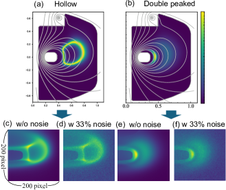
Figure 5: The phantom distributions and their projected images. (a) is labeled the ’hollow’ distribution, and (c) is the projected results with (a) using the geometry matrix $H$, and (d) includes 33% added noise (for example) from (c). Similarly, (b) is labeled ’double peaked’, (e) shows its projected results, and (f) shows the same data with added noise.

The performance of tomography with log-GPT using phantom was evaluated. Two model distributions with (a) hollow and (b) double-peaked, which are usually observed in RT-1 plasmas, were prepared as phantoms, as shown in Fig. 5. The test input data, denoted as $\bm{g}^{\mathrm{inp}}$, were generated by projecting the phantom data using the geometry matrix $H$ with white Gaussian noise at levels of 1%, 3.3%, 10%, 33%, and 100%. The noise level is defined as the ratio of the standard deviation of the noise $\sigma_{\epsilon}$ to the mean value of the projected data, and is calculated as:

$$\mathrm{noise\,level}\;(\%)=100\times\sigma_{\epsilon}/{\langle\bm{g}\rangle}.$$ (31)

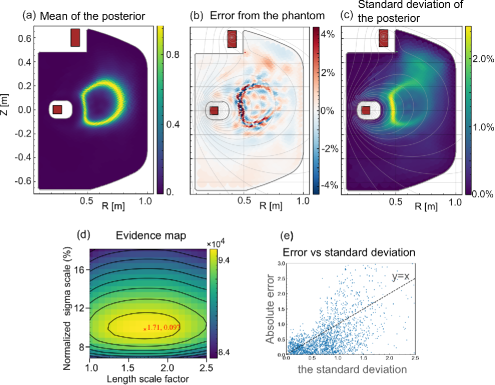
Figure 6: Results of log-Gaussian process tomography when the phantom distribution is “hollow” and the noise level is 10%. (a) Mean of the posterior probability of the local emissivity. (b) Error between the mean posterior value and the true value. (c) Standard deviation of the posterior probability of the local emissivity. (d) Mapping of the evidence, where the optimal point for the hyperparameters has a normalized sigma scale of 9.7% and a length scale factor of 1.71. (e) Relation between the standard deviation (c) and the error (b).

Fig. 6 shows tomographic results of log-GPT for the hollow distribution phantom with the 10% noise level. The hyperparameters of this model are determined by mapping the evidence given in Eq. 24 with respect to the length scale factor $\ell_{S}$ and the sigma scale $\sigma_{S}$, as shown in the Fig. 6(d). The optimized values are $\hat{\ell}_{S}=1.71$ and $\sigma_{S}=9.7\%$, indicating that the optimized length scale corresponds to 1.71 times the referenced length scale distribution in Fig. 3, and the optimized sigma scale is almost the same as the noise level of 10%. The strong effect of the sigma scale on the evidence may be due to the fact that the number of observation data $M$ is considerably larger than the number of inducing points $N$, making the first and fourth terms in Eq. 24 dominant. Fig. 6(a) shows the mean of the posterior probability of the local emissivity, which is the tomographic result. Fig. 6(b) shows the residual error distribution from the true distribution. Fig. 6(c) shows the standard deviation of the posterior. The standard deviation reflects the uncertainty in the emissivity distribution, as shown in Fig. 6(e), which is important for evaluating the tomographic results.

5.2 Comparison with Other Methods

To evaluate the performance of the proposed log-GP method, we compare it with the standard GPT and the MFI. The log-GPT with a uniform length scale was also used to investigate the influence of the length scale distribution. The input data were based on the phantom distributions labeled “hollow” and “double peaked,” as shown in Fig. 5. The noise levels range from 1% to 100%. The standard GPT and the log-GPT are executed under the same setting on inducing points, kernel functions, and sigma scale. The length scale factor $\hat{\ell}_{S}$ was consistently set at 1.71 for each condition, and the sigma scale $\sigma_{S}$ was assigned a value equivalent to the input noise levels. The log-GP with uniform length scale and MFI use the same input points with a grid structure, where the interval is 1 cm and the size is $80\times 100$. The hyperparameters for the MFI were optimized to minimize the total error defined in Eq. 32. For the uniform length scale, $\ell$ = 4.2 cm was adopted, where the evidence was the largest. The regularization parameter $\lambda$ in MFI was selected to minimize the total reconstruction error in each condition, which is defined as follows:

$$\mathrm{total\;error}\;(\%)=100\times\sqrt{\langle|\tilde{f}-{f}_{\mathrm{true}}|^{2}\rangle}/\sqrt{\langle{{f}_{\mathrm{true}}^{2}}\rangle}.$$ (32)

Table 1: Comparison of accuracy between four tomographic methods: standard GPT, log-GPT with non-uniform length scale, log-GPT with uniform length scale, and MFI. The types are separated into hollow and double peaked, and the noise levels are varied from 1% to 100%. Each entry represents the total reconstruction error (%) as defined in Eq.32. Bold numbers indicate the most accurate value under the same condition.

		Noise level
Method	Distribution type	1%	3.3%	10%	33%	100%
Standard GPT	hollow	5.5	8.0	10.	15.	21.
log-GPT (non-uniform)	hollow	2.3	3.4	5.2	8.2	13.
log-GPT (uniform)	hollow	3.0	3.7	5.5	8.5	13.
MFI	hollow	2.3	3.8	8.0	12.	19.
Standard GPT	double peaked	3.7	7.0	9.9	13.	20.
log-GPT (non-uniform)	double peaked	2.9	3.8	6.8	8.1	14.
log-GPT (uniform)	double peaked	6.6	7.2	8.6	11.	17.
MFI	double peaked	3.7	5.4	7.9	14.	23.

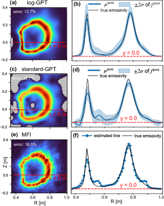
Figure 7: The results of the comparison between three methods, where the noise level of the input image is 100% in each method. The top (a,b), middle (c,d) and bottom (e,f) rows show the results of log GPT, standard GPT and MFI, respectively. The left figures (a, c, e) show the two-dimensional distributions of the estimated values, and the right figures (b, d, f) show the radial profiles of the emissivity at $Z=0$ m. The regions below 0 are masked in gray, as shown in (b). The black lines on the right represent the true distribution, and the red dashed lines indicate the zero value.

The results of the comparison are summarized in Table 1, which demonstrates that the proposed method, log-GPT, has the smallest total error in every case. It is noteworthy that although the MFI deliberately optimizes the hyperparameter for the best accuracy, log-GPT still outperforms it. However, it should be noted that comparing GPT to MFI is not entirely fair because the length scale distribution of GPT, ${\ell}(\vec{r})$, is adjusted to fit any local distribution associated with RT-1, as shown in Fig. 3.

Additionally, Fig. 7 specifically displays the tomographic results at a 100% noise level for the three methods. Comparing Figs. 7(a), (c), and (e), the standard GPT shows a smoother distribution than the log-GPT despite using the same length scale, and the MFI exhibits a noise-like distribution. It is evident that the MFI solution would be smoother with a larger $\lambda$, but this would likely result in a larger error. From Fig. 7(c), we can recognize that the standard GPT solution violates the physical constraint that it is locally greater than zero. Even if the mean value is greater than zero, as shown in Fig. 7(f), the MFI method may still violate the constraint when the variance is considered, which can complicate subsequent analyses, including error propagation.

5.3 Discussion

The accuracy of tomographic methods using Bayesian theorem depends on how well the prior distribution captures the possible plasma distributions. The superior accuracy of the log-GPT observed in this study is likely due to the fact that it inherently represents plasma distributions more naturally than the standard GPT. However, it should be noted that the proposed method requires more computational time compared to conventional methods, mainly due to the iterative nature of the Newton-Raphson method.

The log-GPT and MFI methods share a conceptual similarity as in the MFI method; the regularization weight for smoothing is inversely proportional to the amplitude (Eq. 4), while in the log-GPT method, the standard deviation of the gradient is proportional to the amplitude (Eq. 14). However, GPT allows us to optimize the regularization intensity and smoothness through the sigma scale and length scaleparameters independently, which is advantageous for inverse transform of localized structures with noise signals. In this respect, log-GPT combines the advantages of both GPT and MFI, providing a more flexible and robust framework for plasma tomography.

The present study just simulates the tomographic reconstruction of visible light measurements from a tangential view in the RT-1 instrument, it is based on idealized numerical experiments. In actual visible light measurements, the effect of reflections from wall should be carefully considered in future studies to ensure the applicability of the method to real-world scenarios.

6 Conclusion

We proposed a novel tomographic method, nonlinear-GPT using Laplace approximation, focusing on implementing log-GPT to ensure non-negativity. Inducing points were used to improve computational efficiency, and the local emissivity on the poloidal cross-section was reconstructed from line-integrated emissivity data. The effectiveness and performance of this approach were demonstrated through a case study based on the RT-1 device configuration. Accuracy validation using phantom data revealed that the proposed method outperforms existing tomographic methods, including standard GPT and MFI.

References

References

- [1] Ingesson L, Alper B, Chen H, Edwards A, Fehmers G, Fuchs J, Giannella R, Gill R, Lauro-Taroni L and Romanelli M 1998 Nuclear Fusion 38 1675 URL https://dx.doi.org/10.1088/0029-5515/38/11/307
- [2] Odstrčil T, Pütterich T, Odstrčil M, Gude A, Igochine V, Stroth U and Team A U 2016 Review of Scientific Instruments 87 123505 ISSN 0034-6748 (Preprint https://pubs.aip.org/aip/rsi/article-pdf/doi/10.1063/1.4971367/14711712/123505_1_online.pdf) URL https://doi.org/10.1063/1.4971367
- [3] Jardin A, Bielecki J, Mazon D and et al 2021 Eur. Phys. J. Plus 136 706 URL https://doi.org/10.1140/epjp/s13360-021-01483-z
- [4] Svensson J 2011 JET Internal report URL https://scipub.euro-fusion.org/wp-content/uploads/eurofusion/EFDP11024.pdf
- [5] Li D, Svensson J, Thomsen H, Medina F, Werner A and Wolf R 2013 Review of Scientific Instruments 84 083506 ISSN 0034-6748 (Preprint https://pubs.aip.org/aip/rsi/article-pdf/doi/10.1063/1.4817591/14781552/083506_1_online.pdf) URL https://doi.org/10.1063/1.4817591
- [6] Chilenski M A, Greenwald M, Marzouk Y, Howard N T, White A E, Rice J E and Walk J R 2015 Nucl. Fusion 55 023012
- [7] Leddy J, Madireddy S, Howell E and Kruger S 2022 Plasma Phys. Controlled Fusion 64 104005
- [8] Michoski C, Oliver T A, Hatch D R, Diallo A, Kotschenreuther M, Eldon D, Waller M, Groebner R and Nelson A O 2024 Nucl. Fusion 64 035001
- [9] Wang T, Mazon D, Svensson J, Li D, Jardin A and Verdoolaege G 2018 Review of Scientific Instruments 89 063505 ISSN 0034-6748 (Preprint https://pubs.aip.org/aip/rsi/article-pdf/doi/10.1063/1.5023162/15910541/063505_1_online.pdf) URL https://doi.org/10.1063/1.5023162
- [10] Wang T, Mazon D, Svensson J, Li D, Jardin A and Verdoolaege G 2018 Review of Scientific Instruments 89 10F103 ISSN 0034-6748 (Preprint https://pubs.aip.org/aip/rsi/article-pdf/doi/10.1063/1.5039152/16725857/10f103_1_online.pdf) URL https://doi.org/10.1063/1.5039152
- [11] Wang T, Mazon D, Svensson J, Liu A, Zhou C, Xu L, Hu L, Duan Y and Verdoolaege G 2019 J. Fusion Energy 38 445–457
- [12] LI B, WANG T, NIE L, LONG T, LIU Z, WU H, KE R, WANG Z, YU Y and XU M 2021 Plasma Science and Technology 23 095104 URL https://dx.doi.org/10.1088/2058-6272/ac0490
- [13] Gibbs M 1997 Bayesian Gaussian Processes for Regression and Classification. Ph.D. thesis University of Cambridge
- [14] Ertl K, Linden W v d, Dose V and Weller A 1996 Nucl. Fusion 36 1477–1488
- [15] Rasmussen C E and Williams C K I 2005 Gaussian Processes for Machine Learning (Adaptive Computation and Machine Learning) (The MIT Press) ISBN 026218253X
- [16] Møller J, Syversveen A and Waagepetersen R 1998 Scand. Stat. Theory Appl. 25
- [17] Ryter F, Leuterer F, Pereverzev G, Fahrbach H U, Stober J, Suttrop W and Team A U 2001 Phys. Rev. Lett. 86(11) 2325–2328 URL https://link.aps.org/doi/10.1103/PhysRevLett.86.2325
- [18] Bielecki J 2018 J. Fusion Energy 37 201–210
- [19] Kuss M and Rasmussen C E 2005 Journal of Machine Learning Research 6 1679–1704 URL http://jmlr.org/papers/v6/kuss05a.html
- [20] Williams C and Barber D 1998 IEEE Transactions on Pattern Analysis and Machine Intelligence 20 1342–1351 URL https://ieeexplore-ieee-org.utokyo.idm.oclc.org/document/735807
- [21] Minka T P 2001 A family of algorithms for approximate Bayesian inference Ph.D. thesis Massachusetts Institute of Technology. Department of Electrical Engineering and Computer Science URL http://hdl.handle.net/1721.1/86583
- [22] Gibbs M and Mackay D 2000 IEEE Transactions on Neural Networks 11 1458–1464
- [23] Fujii K, Yamada I and Hasuo M 2018 Fusion Sci. Technol. 74 57–64
- [24] Ueda K, Nishiura M, Kenmochi N, Yoshida Z and Nakamura K 2021 Review of Scientific Instruments 92 073501 ISSN 0034-6748 (Preprint https://pubs.aip.org/aip/rsi/article-pdf/doi/10.1063/5.0043875/16017295/073501_1_online.pdf) URL https://doi.org/10.1063/5.0043875
- [25] YOSHIDA Z, OGAWA Y, MORIKAWA J, WATANABE S, YANO Y, MIZUMAKI S, TOSAKA T, OHTANI Y, HAYAKAWA A and SHIBUI M 2006 Plasma and Fusion Research 1 008–008 URL https://doi.org/10.1585/pfr.1.008
- [26] Nishiura M, Yoshida Z, Saitoh H, Yano Y, Kawazura Y, Nogami T, Yamasaki M, Mushiake T and Kashyap A 2015 Nuclear Fusion 55 053019 URL https://dx.doi.org/10.1088/0029-5515/55/5/053019
- [27] Nishiura M, Yoshida Z, Kenmochi N, Sugata T, Nakamura K, Mori T, Katsura S, Shirahata K and Howard J 2019 Nuclear Fusion 59 096005 URL https://doi.org/10.1088/1741-4326/ab259a
- [28] Nishiura M, Kawazura Y, Yoshida Z, Kenmochi N, Yano Y, Saitoh H, Yamasaki M, Mushiake T, Kashyap A, Takahashi N, Nakatsuka M and Fukuyama A 2017 Nuclear Fusion 57 086038 URL https://doi.org/10.1088/1741-4326/aa720d
- [29] Saitoh H, Nishiura M, Kenmochi N and Yoshida Z 2024 Nat. Commun. 15 861 URL https://doi.org/10.1038/s41467-024-44977-x
- [30] KENMOCHI N, NISHIURA M, NAKAMURA K and YOSHIDA Z 2019 Plasma and Fusion Research 14 1202117–1202117
- [31] Snelson E and Ghahramani Z 2005 Sparse gaussian processes using pseudo-inputs Advances in Neural Information Processing Systems vol 18 ed Weiss Y, Schölkopf B and Platt J (MIT Press) URL https://proceedings.neurips.cc/paper_files/paper/2005/file/4491777b1aa8b5b32c2e8666dbe1a495-Paper.pdf
- [32] Xu S, Wang T, Tieulent R, Colette D, Mazon D, Verdoolaege G and Li J 2024 Plasma Phys. Controlled Fusion 66 065010