Conditional Density Estimation with Histogram Trees

Abstract

Conditional density estimation (CDE) goes beyond regression by modeling the full conditional distribution, providing a richer understanding of the data than just the conditional mean in regression. This makes CDE particularly useful in critical application domains. However, interpretable CDE methods are understudied. Current methods typically employ kernel-based approaches, using kernel functions directly for kernel density estimation or as basis functions in linear models. In contrast, despite their conceptual simplicity and visualization suitability, tree-based methods—which are arguably more comprehensible—have been largely overlooked for CDE tasks. Thus, we propose the Conditional Density Tree (CDTree), a fully non-parametric model consisting of a decision tree in which each leaf is formed by a histogram model. Specifically, we formalize the problem of learning a CDTree using the minimum description length (MDL) principle, which eliminates the need for tuning the hyperparameter for regularization. Next, we propose an iterative algorithm that, although greedily, searches the optimal histogram for every possible node split. Our experiments demonstrate that, in comparison to existing interpretable CDE methods, CDTrees are both more accurate (as measured by the log-loss) and more robust against irrelevant features. Further, our approach leads to smaller tree sizes than existing tree-based models, which benefits interpretability.

1 Introduction

Conditional density estimation (CDE) is a crucial yet challenging task in modeling the associations between the features and the continuous target variable, which has received a lot of research interest since the 1970s [44]. By modeling the full conditional distribution, CDE is useful when the datasets are multi-modal, heavily skewed, or heteroscedastic. As a result, it is widely applied in various fields, including Genome [8], Astronomy [3], wind power forecasting [19], and computer network [47].

CDE provides richer information for data understanding than regression, which only models the conditional mean. This makes CDE desirable for well-informed decision-making in critical areas, such as healthcare [32, 53, 14], which calls for interpretability.

Despite its importance, recent CDE research has predominantly focused on black-box models, such as neural networks [10, 55, 39, 46, 50] and tree ensembles [13]. In contrast, intrinsically interpretable models for CDE are understudied. Specifically, decision tree-based methods are largely neglected, with CADET [6] being the only existing method to the best of our knowledge. However, CADET’s assumption of a Gaussian distribution for the target variable in each leaf node limits its ability to model complex conditional densities.

As a result, kernel-based models became the standard among ‘shallow’ models for CDE, including methods based on kernel density estimation (KDE) [44], and linear models with the basis functions chosen as Gaussian kernels [54, 11]. Nevertheless, kernel-based models are arguably less interpretable than decision trees: as conditions in decision trees are directly readable, they are comprehensible to humans without statistical expertise (e.g., individuals affected by data-driven decisions rather than professional data analysts).

To address these limitations, we propose the Conditional Density Tree (CDTree), a flexible tree-based CDE model in which each leaf node consists of a histogram model. For illustration, Figure 1 shows the CDTree learned from a dataset about the personal medical cost with demographic features [24]. The figure visualizes the histogram models for the conditional densities on three selected leaf nodes, along with the unconditional density. The readable rules, extracted from the tree paths, and the histogram visualizations, make the results easily comprehensible to humans without statistical expertise. For instance, the difference in medical costs between smokers and non-smokers is evident when comparing the plots. The full results with histograms on all leaf nodes, as well as further descriptions of the dataset, are provided in Appendix E.

Learning a CDTree from data is a challenging task, as it requires simultaneously optimizing the decision tree structure and the number of bins for histograms on all leaf nodes. While often used for either task, cross-validation is too time-consuming if we need to search for the optimal number of bins for every possible node split. Thus, we formalize the learning problem using the minimum description length (MDL) principle [16, 41], which we briefly review in Section 4.1. Adopting MDL eliminates the need for tuning the hyperparameter, by cross-validation, for both regularizing the decision trees [5] and for choosing the number of bins for histograms.

Our main contributions are as follows. First, we introduce the CDTree for the CDE task and formalize the learning problem with the MDL principle. Second, we propose an iterative algorithm that can search the optimal histogram for all possible node splits. Third, we benchmark against a wide range of competitors and demonstrate that CDTree is highly competitive. Specifically, CDTree is more accurate than existing interpretable CDE methods (as measured by the log-loss). Meanwhile, CDTree has smaller tree sizes than other tree-based methods, which benefits interpretability. In addition, CDTree is extremely robust to irrelevant features, which is noteworthy as irrelevant features are known to harm the convergence rate for CDE [17]. Further, we argue that the (intrinsic) explanations of CDTree are trustworthy only if the CDTree is robust against irrelevant features.

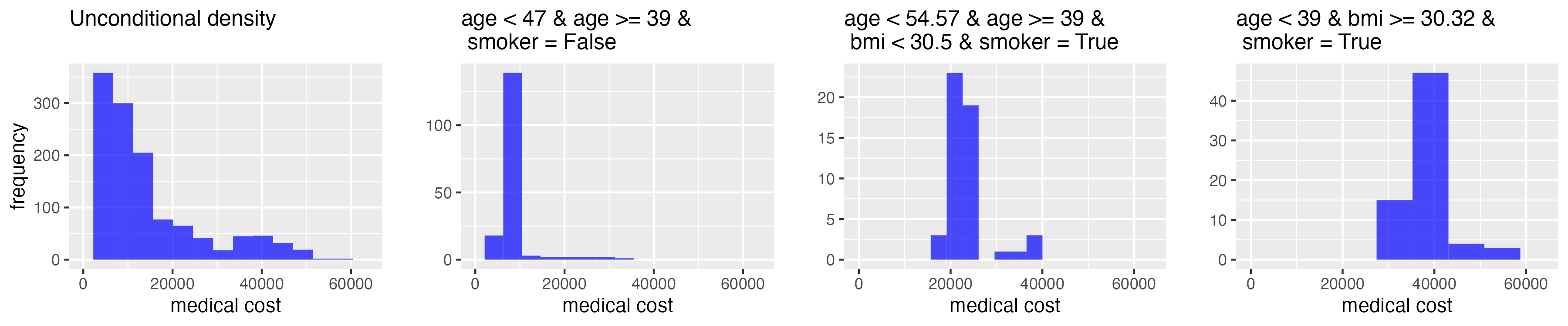
Figure 1: Three selected leaves from the CDTree modeling the conditional density of the medical costs given demographic features, together with the unconditional density for medical costs.

2 Related Work

KDE-based CDE. Several CDE methods have been developed based on kernel density estimation (KDE). The most straightforward approach, known as conditional-KDE (CKDE) [44], involves separately estimating the joint and marginal densities using unconditional KDE and then taking their ratio to obtain the conditional density. Another approach, $\epsilon$-neighborhood KDE (NKDE), estimates the conditional density by applying KDE to the subset of data points within the $\epsilon$-neighborhood of the target point, with the range of the neighborhood controlled by the parameter $\epsilon$.

However, KDE-based methods have several limitations. First, KDE is arguably less interpretable than tree-based models, as understanding KDE requires statistical knowledge, making it less accessible to domain experts and the general public. Additionally, while decision trees can naturally handle both discrete and continuous feature values, discrete features pose significant challenges for kernel-based methods. Specifically, CKDE requires estimating the joint density of the features and target variable, which necessitates the use of discrete kernels for discrete variables. These discrete kernels are often difficult to interpret [31]. As for NKDE, when both discrete and continuous feature values exist, the choice of the scale for the continuous variables unavoidably introduces a certain degree of arbitrariness in defining the distances used to characterize the neighborhood.

Regression-based CDE. Motivated by several issues of CKDE, including high variance as a plug-in estimator, the exponentially growing search space for bandwidth tuning, and the curse of dimensionality for estimating the joint density function, the method named least-squares CDE (LSCDE) [54] was proposed. LSCDE aims to directly estimate the ratio between the joint and marginal densities by assuming this ratio is a linear combination of several basis functions, chosen to be Gaussian kernels. Similarly, Fan et al. [11] proposed double-kernel local linear regression, which transforms the conditional density function into the conditional expectation of the (unconditional) density function of the target variable, leading to a least-squares approach as well. However, both methods face the challenge of bandwidth selection, as the value of the Gaussian kernel function must be calculated with the entire feature vector as input. This issue becomes particularly problematic as the search space for the bandwidth grows exponentially with the number of features.

Tree-based CDE. The only existing CDE method based on single trees that we are aware of is CADET [6], which improves CART regression trees [5] by designing a node-splitting heuristic specifically for CDE. However, CADET assumes a Gaussian distribution for the target variable on each leaf, which is far less flexible than our non-parametric histogram models.

Black-box CDE. Neural networks have been shown to perform well in a wide range of tasks. For CDE, the most well-known methods include NF [39] and MDN [4]. As for tree ensemble models, RFCDE [35] first fits a standard random forest, and then estimates the CDE by the weighted average of the unconditional density estimates obtained via KDE, with weights determined by the random forest. Furthermore, the recently proposed LinCDE [13] method learns a boosted tree model based on Lindsey’s method [25]. While black-box models are highly accurate, we argue that interpretable CDE methods are valuable for applications in critical domains and for understanding the data.

3 Conditional Density Tree with Histograms

Tree-based models divide the feature space into disjoint (hyper-)boxes by recursively splitting on individual feature variables (for which we consider binary splits only). Consequently, the induced partition with $K$ subsets (leaves) can be represented as $M=\{S_{k}\}_{k\in[K]}$, where each leaf $S_{k}$ represents a subset of the feature space and $[K]:=\{1,...,K\}$. Further, each leaf is equipped with a single (unconditional) density estimator, denoted as $f_{k}(.)$. Thus, for a dataset $D=(x^{n},y^{n})$ with sample size $n$, the tree-based model $M$ first identifies the leaf to which each $(x,y)\in D$ belongs, and then estimates the conditional density $f(y|x)$ as $f_{k}(y)$ (assuming $x\in S_{k})$.

We choose histograms as our model class for each $f_{k}(.)$. Unlike previous parametric models [13, 6], which carry the risk of misspecification, histograms are non-parametric yet efficient. Additionally, in comparison to KDE, histograms do not require selecting a kernel or tuning the bandwidth.

We next describe our notations and formally present the histogram as a probabilistic model. Formally, a (fixed) histogram model partitions the domain of the target variable $Y$ into equal-width bins, and then approximates the density of $Y$ by piece-wise constants estimated from data. Thus, we can denote a histogram model as a tuple $H=(B_{l},B_{u},h)$, with $B_{l}$ and $B_{u}$ respectively representing the lower and upper boundary of the histogram, and $h$ the number of bins. A histogram model $H$ can parameterize a family of distributions by $\alpha=(\alpha_{1},...,\alpha_{h})$, with the probability density function in the form of $f_{H}(Y=y)=\frac{\alpha_{j}}{(B_{u}-B_{l})/h},\,\,\,\forall y\in[B_{l}+(j-1)\frac{B_{u}-B_{l}}{h},B_{l}+j\frac{B_{u}-B_{l}}{h})$, in which $(B_{u}-B_{l})/h$ is the bin width and $[B_{l}+(j-1)\frac{B_{u}-B_{l}}{h},B_{l}+j\frac{B_{u}-B_{l}}{h})$ denotes the interval for the $j$th bin. In practice, the histogram boundaries $B_{l}$ and $B_{u}$ are often set based on the dataset at hand, by prior knowledge, or by the range of the values plus/minus a small constant. Meanwhile, the parameters $\alpha$ can be estimated by the maximum likelihood estimator (i.e., by the empirical frequencies in each bin): $\hat{\alpha}_{j}=\frac{1}{n}{\sum_{i=1}^{n}\mathbf{1}_{[B_{l}+(j-1)\frac{B_{u}-B_{l}}{h},B_{l}+j\frac{B_{u}-B_{l}}{h})}(x_{i})}$, in which $\mathbf{1}(.)$ is the indicator function.

4 The MDL-optimal CDTree

We briefly review the minimum description length (MDL) principle, and then formalize the problem of learning a CDTree that consists of histograms as an MDL-based model selection problem.

4.1 Preliminary: the MDL principle for model selection

Rooted in information theory, the minimum description length (MDL) principle states that the optimal model is the one that can compress the data most [41, 15]. Precisely, given the dataset $D=(x^{n},y^{n})$, the MDL-optimal model is defined as

$$M^{*}=\arg\min_{M\in\mathcal{M}}-\log_{2}P_{M}(y^{n}|x^{n})+L(M),$$ (1)

in which $M$ is a CDTree and $\mathcal{M}$ the model class of all possible CDTrees for our learning task, meanwhile $L(M)$ is the code length (in bits) needed to transmit the model in a lossless manner. According to the Kraft’s inequality [7], $L(M)$ can also be regarded as a prior probability distribution defined on the model class. Further, $P_{M}(.)$ is the so-called universal distribution [15]: as $M$ parameterizes a family of probability distributions, denoted as $P_{M,\theta}$, $P_{M}(.)$ can be regarded as a “representative" distribution such that the maximum regret, defined as $\max_{y^{n}}\{\max_{\theta}\log_{2}P_{M,\theta}(y^{n}|x^{n})-\log_{2}P_{M}(y^{n}|x^{n})\}$, can be bounded by $n\epsilon>0,\forall\epsilon>0$ as $n\rightarrow\infty$ [15], in which the maximum is defined over all possible values for $y^{n}$ in the domain of the target variable. Intuitively, the regret is the difference between the log-likelihood of $P_{M}(y^{n}|x^{n})$ (which does not depend on $\theta$) and the maximum log-likelihood $\max_{\theta}\log_{2}P_{M,\theta}(y^{n}|x^{n})$. For our learning task, $\theta$ is the parameter vector that contains the histogram parameters (i.e., the $\alpha$’s) for all leaf nodes.

The MDL principle has been successfully applied to various data mining and machine learning tasks [12], and specifically to partition-based models, including histograms and classification trees/rules [37, 57, 36, 22]. The MDL framework provides a principled way of regularizing model complexity without any regularization hyperparameter to be tuned. Moreover, as the Bayesian marginal distribution is one specific type of the universal distributions, the MDL-based model selection can also be regarded as a generalization of Bayesian model selection [16].

4.2 Normalized maximum likelihood for CDTrees

The optimal universal distribution under the MDL framework is the so-called normalized maximum likelihood (NML) distribution, defined as [15, 49, 16]

$$P_{M}(y^{n}|x^{n})=\frac{\max_{\theta}P_{M,\theta}(y^{n}|x^{n})}{\int_{y^{n}}\max_{\theta}P_{M,\theta}(y^{n}|x^{n})},$$ (2)

under the condition that the denominator is finite. It can be shown that the NML distribution is the only distribution that leads to the minimax regret $\min_{P_{M}}\max_{y^{n}}\{\max_{\theta}\log_{2}P_{M,\theta}(y^{n}|x^{n})-\log_{2}P_{M}(y^{n}|x^{n})\}$, in which the denominator in Eq. 2 is exactly equal to the regret [15].

The denominator in Eq. 2 is in general prohibitively expensive to compute [15, 51, 43], with a few exceptions including the cases when the probabistic model represents categorical distributions [21], decision rules for classification [57], and one- and multi-dimensional histogram models [22, 28, 58]. We extend these previous results and prove that, for CDTrees with histogram models, the denominator (regret) is finite and is equal to the products of the regret terms of the NML distributions for one-dimensional histogram models, as shown in Proposition 1. This result is useful for efficiently calculating the denominator (regret) in Eq. 2 for CDTree models, as the regret terms for histogram models are known to be equal to that of the categorical distributions [20, 21], for which an efficient algorithm exists with sub-linear time complexity [30].

Proposition 1.

Let $\theta=(\alpha^{1},...,\alpha^{K})$ be the histogram parameters for histograms on all leaves, and let $\hat{\theta}=\arg\max_{\theta}P_{M,\theta}(y^{n}|x^{n})$. Then $\int_{y^{n}}\max_{\theta}P_{M,\theta}(y^{n}|x^{n})=\prod_{k\in[K]}\mathcal{R}(N_{k},h_{k})$, in which $\mathcal{R}(N_{k},h_{k})$ is the regret (denominator) of the NML distribution of the histogram model on the $k$th leaf node that contains $N_{k}$ data points and $h_{k}$ bins.

We defer the proof to Appendix A due to space limitations.

4.3 Code length for the model

To encode a CDTree model in a lossless manner, we need to sequentially encode 1) the number of nodes in the decision tree, 2) the structure of the tree, 3) the splitting condition for each internal node in a predetermined order (e.g., depth first), 4) the number of bins for the histogram on each leaf node, and 5) the boundaries $B_{l}$ and $B_{u}$ of the histograms. That is, let $L(.)$ denote the function that calculates code length in bits, the code length needed to encode a model $M$ can be decomposed to

$$L(M)= L(\text{\# leaves})+L(\text{tree structure})+\sum_{j\in[K-1]}L(\text{splitting condition of the $j$th \emph{internal} node})$$ (3)

$$+\sum_{k\in[K]}L(\text{\# bins of histogram on the $k$th \emph{leaf} node})+L(\{B_{l},B_{u}\});$$

we next describe them in order.

Encoding the tree size and structure. As we consider full binary trees only, it is sufficient to encode the number of leaves $K$, which also determines the number of total nodes. As $K$ is a positive integer, we adopt the standard Rissanen’s integer universal code [42], denoted as $L_{\mathbf{N}}(K)$, for which the code length is equal to $L_{\mathbf{N}}(K)=c+\log_{2}(K)+\log_{2}\log_{2}(K)+...$; the summation continues until a small enough precision is reached, and $c\approx 2.865$ is a constant.

Further, for full binary trees, the number of all possible tree structures for trees with $K$ leaves is equal to the Catalan number, denoted as $\mathcal{C}_{K-1}$ [52]. Hence, specifying one certain structure costs $\log_{2}\mathcal{C}_{K-1}$ bits. Thus, $L_{\mathbf{N}}(K)+\log_{2}\mathcal{C}_{K-1}$ bits are required for encoding the tree size and structure.

Note that while there exist multiple ways of encoding tree size and structure (e.g., one alternative is to leverage the joint probability of the tree size and the tree structure, which can be defined by treating the tree as a realization of a Galton-Watson process [33, 2]), our encoding scheme adheres to the principle of achieving conditional minimax [16] by explicitly putting a prior on the number of nodes.

Encoding the splitting conditions. An individual splitting condition on a single tree node consists of a variable name and a splitting value, which we encode sequentially.

To begin with, if the dataset contains $m$ feature variables, encoding the name of a certain variable $X$ costs $\log_{2}{m}$ bits. Further, the code length needed for encoding the splitting value depends on the variable type. First, for a discrete variable $X$ with $|\mathcal{X}|$ unique values, specifying a single value cost $\log_{2}(|\mathcal{X}|)$ bits. Second, encoding the splitting value for a continuous variable can be achieved by sequentially encoding 1) the granularity level for the search space, denoted as the positive integer $d$, and 2) the exact value within the granularity level $d$. Specifically, with a fixed $d$, we consider as the search space the $C\cdot 2^{d-1}$ quantiles that can partition the values of $X$ into equal-frequency bins. Note that the values of $X$ are based on the subset of data points contained in this internal node locally.

Hence, encoding $d$ costs $L_{\mathbf{N}}(d)$ bits with the Rissanen’s code [42], and encoding one specific splitting value (quantile) costs $\log_{2}(C\cdot 2^{d-1})=\log_{2}(C)+d-1$ bits. That is, we treat the granularity level $d$ as a parameter to be optimized when learning a CDTree from the data, which avoids (arbitrarily) specifying the granularity in advance, a shortcoming in previous MDL-based methods (for other tasks instead of CDE) [22, 36, 58, 57, 28]. In contrast, the parameter $C$ can be used to express the prior belief about the hierarchical structure of the search space, as further discussed in Appendix C.3.

Encoding the histograms. One subtle choice we made is to set the boundaries for histograms on all leaves to be same, and we set them as the global boundary of the target variable. This avoids unseen (test) data points falling outside the boundaries of the histograms on the leaf nodes. This is because while it may be common to assume that the boundaries for the histogram are known in unconditional density estimation, assuming the same for CDE is hardly realistic.

Therefore, the code length needed to encode the boundary $L(\{B_{l},B_{u}\})$ in Eq. 3 is a constant that does not affect the model selection result. Consequently, it suffices to encode the number of bins for each histogram: for the histogram on the $k$th leaf with $h_{k}$ bins, it costs $L_{\mathbf{N}}(h_{k})$ bits by the Rissanen’s integer code [42].

4.4 Model selection criterion

Combining Eq. 1,2, and 3, together with the results from Proposition 1, we present the following MDL-score as our final model selection criterion:

$$M^{*}=\arg\min_{M\in\mathcal{M}}-\log_{2}\left(\max_{\theta}P_{M,\theta}(y^{n}|x^{n})\right)+\sum_{k\in[K]}\log_{2}\mathcal{R}(N_{k},h_{k})+L(M)$$ (4)

which has the form of the regularized maximum likelihood, yet without the need to tune the regularization hyperparameter. Note that the exact form of $L(M)$ depends on the types of the feature variables; e.g., by assuming all variables are continuous, we obtain

$$L(M)=L_{\mathbf{N}}(K)+\log_{2}\mathcal{C}_{K-1}+\sum_{j\in[K-1]}\left(\log_{2}(m)+L_{\mathbf{N}}(d_{j})+\log_{2}(C)+d_{j}-1\right)+\sum_{k\in[K]}L_{\mathbf{N}}(h_{k}),$$

where, as defined previously, $\mathcal{R}(.)$ denotes the regret term of each histogram, $L_{\mathbf{N}}(.)$ the Rissanen’s integer universal code [42], $m$ the number of feature variables, $d_{j}$ the granularity level for the search space for the splitting values corresponding to the $j$th internal node, $C$ the constant that controls the hierarchical structure of the search space of the splitting values, and $h_{k}$ the number of bins for the histogram on the $k$th leaf node.

5 Algorithm

While finding the optimal tree-based model with the branch-and-bound approach is possible for regression [59] and classification [18], it does not apply to our task for two reasons. First, our MDL-based regularization term differs from traditional penalty terms based on tree size. Second, our task resembles optimizing model trees [27, 38] rather than classification and regression trees, as we aim to find the optimal histogram for each candidate split.

Input: Training dataset $D$

Output: CDTree $M$

$M\leftarrow\{S_{0}\}$ ;

  // One leaf node only

1 while True do

2       for $S\in M$ do

             Search the condition that splits $S$ into two nodes and minimizes the MDL-score (Eq. 4). ;

              // Described in detail in Algorithm 2

3            

4       end for

5      if Splitting any $S\in M$ cannot further decrease the MDL-score then

6             return CDTree $M$

7      else

8             Among all $S\in M$, find the single $S^{*}$ to be split that minimizes the MDL-score.

9            Update $M$ by replacing $S^{*}$ with its two child nodes that minimize the MDL-score.

10       end if

11      

12 end while

Algorithm 1 Learn CDTree from data

A greedy approach for tree construction. We thus take a heuristic approach to optimize our MDL-score in Eq. 4. As summarized in Algorithm 1, we start with a tree with one leaf node $M=\{S_{0}\}$; next, we iteratively update $M$ by replacing one of the leaf nodes with its ‘best’ two child nodes. Specifically, to achieve the lowest MDL-score at each iteration, we simultaneously search for 1) which node to split, 2) the splitting condition for that node, and 3) the optimal number of bins for the histograms. That is, we iterate over all leaf nodes in $M$; for each leaf node, we search for the splitting condition, along with the number of bins for the histograms on the (potential) child nodes, which as a whole minimizes the MDL-score. Notably, while an exhaustive search for the ‘best’ models on all potential child nodes is considered infeasible in traditional model tree methods [27, 38], we empirically demonstrate in Section 6.5 that our algorithm is comparable to KDE-based methods.

Finding the child nodes. We next elaborate on the search for the tree-splitting condition at each iteration, for which the pseudo-code is provided in Algorithm 2. For simplicity, we assume all feature variables are either continuous or binary (i.e., categorical features are one-hot encoded in our implementation).

Further, we iterate over all columns of the feature matrix. For each column, we start with the granularity level $d=1$ and generate candidate split points as the $C\cdot 2^{d-1}$ quantiles that lead to equal frequency binning of the values. Note that the quantiles are generated based on the subset of data points covered by the node to be split, rather than the entire dataset. We search for the best split point at the fixed $d$ that yields the minimum MDL score among all generated candidates. We then proceed to the next granularity level $d+1$ and repeat the process, which stops if no split point in the next granularity level results in a better (smaller) MDL score.

Last, we also need to search for the optimal number of bins for the histogram that leads to the minimum MDL score, which we defer to Appendix B.

Input: Training set $D_{S}=(x^{\{S\}},y^{\{S\}})$ covered by node $S$, with $x^{\{S\}}=(\vec{x}_{1},...,\vec{x}_{m})$ having $m$ columns, and constant $C$

Output: The splitting condition of $S$ that minimizes the MDL-score

1 for $j\in\{1,2,...,m\}$ do

2       $d\leftarrow 1$

3      while True do

4             $candidate\_splits\leftarrow$ $\text{The}\,\,C\cdot 2^{d-1}$ quantiles for equal-frequency binning for $\vec{x}_{j}$

5            for $s\in candidate\_splits$ do

                   $D_{l}\leftarrow\{(x,y)\in D_{S}|x_{j}\leq s\}$ ;

                    // Always $s=1/2$ for binary features

6                  

7                  $D_{r}\leftarrow\{(x,y)\in D_{S}|x_{j}>s\}$

                  Construct histograms for $D_{l}$ and $D_{r}$ that minimize the MDL-score conditioned on the fixed $j$ and $d$. ;

                    // Described in detail in Algorithm 3

8                  

9                  Score $\leftarrow$ Calculate the MDL-score assuming $D_{S}$ is split into $D_{l}$ and $D_{r}$

10             end for

11            

12            if The best Score is worse than that of the previous d then  Break; else $d\leftarrow d+1$ ;

13            

14       end while

15      Record the best tuple $(d,s)$ for this column index $j$

16 end for

return The tuple $(j,d,s)$ that minimize the MDL-score

Algorithm 2 Find the best split for node $S$

6 Experiments

We present our experiments to demonstrate the empirical performance of CDTree from various perspectives. Specifically, we aim to answer the following research questions: 1) Does CDTree provide more accurate conditional density estimation compared to existing interpretable (tree-based and kernel-based) methods? 2) As a proxy for interpretability, does CDTree has smaller tree size in comparison to other tree-based models? 3) Is CDTree robust against irrelevant "noisy" features? 4) Are the runtimes of our algorithm comparable to those of kernel-based methods?

6.1 Experiment setup

We use 14 datasets with numerical target variables from the UCI repository [1]. These datasets, summarized in Table 1, cover a wide range of sample sizes and dimensionalities. We benchmark our method against a variety of competitors, with all results obtained on the test sets using five-fold cross-validation. Our competitors include 1) NKDE and CKDE [44, 46], which are based on kernel density estimation, with bandwidth and $\epsilon$ (for NKDE only) tuned by cross-validation; 2) LSCDE [54], which directly estimates the ratio of joint and marginal density using linear models with Gaussian kernel basis functions; 3) the tree-based method CADET [6], which fits a Gaussian distribution on each leaf node; 4) two more tree-based baselines introduced by us, CART-k and CART-h, which respectively fits a KDE model and a histogram after a CART regression tree [5] is learned from data.

Furthermore, we compare against three black-box models as "upper" baselines, including 1) neural network methods NF [39] and MDN [4], which apply both dropout and noise regularization [45], and 2) the recently proposed tree boosting method LinCDE [13]. Nonetheless, our goal with CDTree is not to be more accurate than black-box models, but to introduce a CDE method that is both interpretable and accurate.

Table 1: Datasets from the UCI repository, with the numbers of rows and columns

dataset	energy	synchronou	localizati	toxicity	concrete	slump	forestfire
# rows	9568	557	107	908	1030	103	517
# cols	5	5	6	7	9	10	13
dataset	navalpropo	skillcraft	sml2010	thermograp	support2	studentmat	supercondu
# rows	11934	3338	2764	1003	9105	395	21263
# cols	17	19	21	26	27	44	82

For reproducibility, we provide further details about implementations and parameter choices in Appendix C. We made our source code public: https://github.com/ylincen/CDTree.

6.2 Conditional density estimation accuracy

In Table 2, we report the average negative log-likelihoods (NLL) on the test sets, which can be regarded as an approximation to the expected log-loss $E(-\log(y|x))$, the standard loss function for measuring CDE accuracy.

Table 2: Negative log-likelihoods (smaller is better) on test sets. The best results among interpretable methods are shown in bold, and the best results among all interpretable and black-box models are marked by the underlines. The datasets are ordered by their numbers of columns (ascending).

	Interpretable models							Black-box models
Datasets	CADET	CART-h	CART-k	CKDE	LSCDE	NKDE	Ours	LinCDE	MDN	NF
energy	3.55	3.09	3.06	2.47	3.38	3	2.93	2.93	2.78	2.86
synchrono	-2.93	-1.63	-1.86	-3.59	-1.25	-1.57	-2.11	-1.85	-2.94	-2.64
localizat	-0.23	-0.55	-0.01	-0.26	-0.61	-0.28	-0.66	-0.95	-0.68	-0.43
toxicity	1.8	1.5	1.38	1.32	1.34	1.55	1.53	1.29	1.24	1.23
concrete	4.17	3.75	3.93	3.32	3.66	3.91	3.72	3.47	2.97	3.18
slump	3.42	3.55	3.43	2.35	2.91	3.08	3.34	2.98	2.23	2.39
forestfir	134	3.96	4.39	4.85	4.68	5.55	3.43	4.35	3.26	3.23
navalprop	-3.53	-3.3	-3.66	-2.8	-2.88	-3.19	-3.6	-3.36	-4.12	-3.75
skillcraf	94.4	0.46	-0.42	1.54	1.61	1.56	-1.02	1.26	0.35	1.11
sml2010	6.52	2.85	2.89	1.61	3.14	3.12	2.7	2.97	2.15	2.61
thermogra	2.21	0.66	0.72	0.66	0.94	0.94	0.64	0.59	0.56	0.52
support2	97.3	0.51	0.32	2.09	2.46	2.13	0.29	1.48	1.53	1.24
studentma	3.83	2.65	2.66	2.89	4.19	3.11	2.66	2.59	3.85	3.54
supercond	9.6	3.84	4.36	4.55	4.17	4.19	3.48	3.87	3.33	3.5
rank (all)	8.79	5.68	6.04	5.11	7.46	7.68	4	4.46	2.57	3.21
rank (intp.)	6.07	3.43	3.86	3.14	4.57	4.86	2.07	—	—	—

Comparison to interpretable models. The NLL of the CDTree models are the best (lowest) in 6 out of 14 datasets among all interpretable models, which are shown in bold in the table. Further, among all interpretable models, our average rank is the best, as reported in the (last row) of Table 2. As the datasets are increasingly ranked based on their dimensionalities, we observe that CKDE—although also achieving the best NLL in 6 datasets—only performs well on datasets with low dimensions. Additionally, the other two kernel-based methods LSCDE and NKDE have in general worse accuracy.

Further, CDTree has better accuracy (lower NLL) than all tree-based competitors on almost all datasets (13 out of 14 datasets for CADET, and 12 out of 14 datasets for CART-h and CART-k). The superiority of CDTree highlights the advantages of 1) using non-parametric histogram models, and 2) conducting an exhaustive search for optimal histograms for all node splits when learning the tree structure, rather than fitting the model after the tree structure is fixed, as in CART-h and CART-k.

Comparison to black-box models. Neural network models generally exhibit better accuracy than interpretable models, as indicated by their average ranks. However, their non-transparency limits their applicability in critical areas. We argue that studying interpretable models and introducing CDTree paves the way for developing local surrogate models [40, 26], an essential approach for generating post-hoc explainability for black-box models, as no such method currently exists for CDE.

Further, the performance of CDTree is surprisingly on par with that of LinCDE. Since CDTree is based on a single tree while LinCDE is a tree ensemble model, we conjecture that the on-par performance is caused by the fact that CDTree adopts non-parametric histograms whereas LinCDE takes a parametric approach (with a much more flexible model class than Gaussian though).

We also report the standard deviations of NLL for all methods in Appendix D.1. Our method shows no anomalously large standard deviations, indicating consistent performance across different datasets.

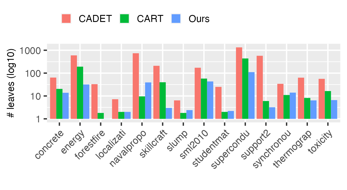
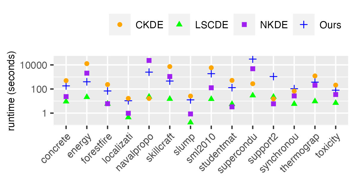
Figure 2: Left: the number of leaves for tree-based methods. Right: Runtimes of CDTree and kernel-based methods. Note that the y-axes are scaled by $\log_{10}(.)$

6.3 Complexity of trees

For tree-based models, the size of the trees is an important proxy for the degree of interpretability [29]. We hence compare the number of leaves of CDTree against the other tree-based models CADET and CART (note that CART-h and CART-k have the same tree structures). We demonstrate in Figure 2 (left) that CDTree has smaller tree sizes than the competitors on most datasets.

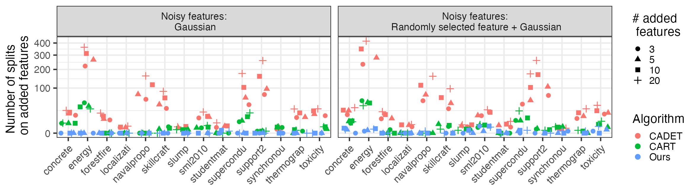
Figure 3: Number of internal nodes with split conditions that contain irrelevant features. The y-axis is scaled by the squared-root for better visualization.

6.4 Robustness to irrelevant features

We next investigate whether CDTree is robust against irrelevant features, which is particularly important for the interpretability of tree-based models, since the (intrinsic) explanation contained in the CDTree would not be trustworthy if such robustness did not hold.

Specifically, we generate ‘noisy’ features in two different ways. The first way is to add $w$ irrelevant features randomly drawn from the standard Gaussian distribution to each dataset. The second way is to first randomly select $w$ features from each dataset; then, for each selected feature $X_{j}$, we generate a ‘noisy’ feature by adding a Gaussian noise to it, i.e., $X_{j}^{\prime}=X_{j}+N(0,s(X_{j})/2)$, where $s(X_{j})$ denotes the estimated standard deviation. We refer to the irrelevant features generated by the first (second) approach as independent (dependent) noisy features, where $w\in\{3,5,10,20\}$ in both cases. Note that adding $X_{j}^{\prime}$ to the dataset does not change the true conditional density as the target variable is conditionally independent of $X_{j}^{\prime}$ given the original feature $X_{j}$.

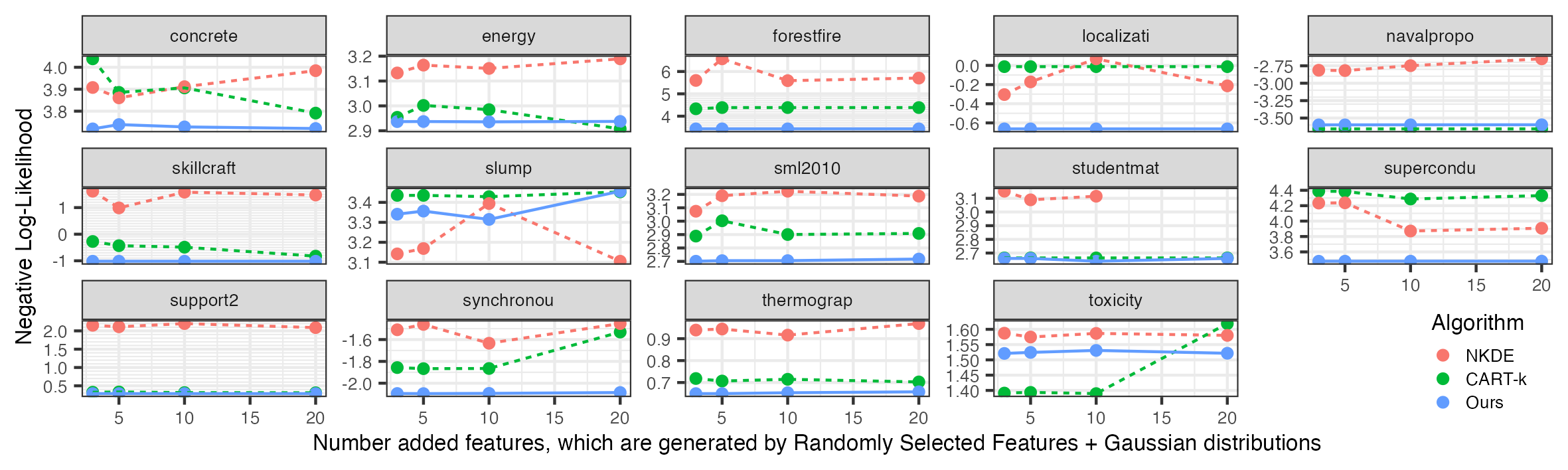
Figure 4: Negative log-likelihoods with different number of irrelevant ‘dependent noisy’ features. The results of CDTree (shown in blue lines) are stable on all datasets.

Next, we train the tree-based models on expanded datasets that include irrelevant features. We count the number of nodes with splitting conditions that involve these added irrelevant features. As demonstrated in Figure 3, the number of splits on irrelevant features for our CDTree is almost always zero for both ways of generating noisy features. In contrast, the tree-based models learned by CART and CADET contain many more nodes with irrelevant features.

We also examine whether the negative log-likelihoods (NLL) remain stable when irrelevant features are added. For ‘dependent noisy’ features, the results are shown in Figure 4, where the NLL of CDTree remains nearly identical regardless of the number of added features—the only exception being the dataset "slump" (with only 103 rows). In contrast, the NLLs obtained by competitor methods are much less stable: the NLL of NKDE varies for most datasets, and CART-k shows visible changes in 6 out of 14 datasets. Similar results are observed when ’independent noisy’ features are added, as shown in Appendix D.2.

6.5 Runtimes

The idea of fitting separate models on the leaves of a decision tree exists since a long time ago [38]. However, it is (still) often believed that fitting separate models for all possible node splits when growing a tree is infeasible. However, we show in Figure 2 (right) the runtime of CDTree and demonstrate that its runtimes are in general lower than the runtimes of CKDE (which requires intensive parameter tuning). While NKDE and LSCDE are in general faster than CDTree, the accuracy of their conditional density estimates are sub-optimal, as discussed previously. We exclude the comparison with other tree-based methods whose implementations are based on CART, as CART is highly optimized and known to be extremely fast. Further, as these tree-based methods either model the conditional means only (CART-h and CART-k) or assume a Gaussian model (CADET), they have far smaller search space, and hence are fast but less accurate.

7 Discussion

In this paper, we studied the interpretable conditional density estimation (CDE) models. Motivated by the fact that tree-based methods are arguably more interpretable than kernel-based methods yet have been largely disregarded for interpretable CDE, we introduced the Conditional Density Tree (CDTree). We formalized the learning problem under the MDL framework, proposed an iterative algorithm, and demonstrated its competitive empirical performance on a wide range of datasets.

Limitations. As histograms are used in the CDTree, we implicitly assume that the support of the target variable is bounded. Hence, the boundaries for the histograms need to be chosen in an ad-hoc way, possibly based on prior knowledge. Further, in practice, it may happen that the unseen data points fall outside the histogram boundary, for which the predicted (conditional) density will be 0, unless the full model is re-trained. We realize that this may cause some issues when using CDTree in practice, but meanwhile, we argue that 1) this is a limitation of the histogram model itself, 2) similar issues could happen in modelling quantiles by the empirical cumulative probability function, as in well-known methods like quantile regression trees and forest, and 3) all probability models have their own (implicit) assumptions on the probability tails, including those specifically designed for modeling the extreme value distributions [9, 23].

Appendix A Proof

Proposition 1. Let $\theta=(\alpha^{1},...,\alpha^{K})$ be the histogram parameters for histograms on all leaves, and let $\hat{\theta}=\arg\max_{\theta}P_{M,\theta}(y^{n}|x^{n})$. Then $\int_{y^{n}}\max_{\theta}P_{M,\theta}(y^{n}|x^{n})=\prod_{k\in[K]}\mathcal{R}(N_{k},h_{k})$, in which $\mathcal{R}(N_{k},h_{k})$ is the regret (denominator) of the NML distribution of the histogram model on the $k$th leaf node that contains $N_{k}$ data points and $h_{k}$ bins.

Proof.

Consider the dataset $D=\{x^{n},y^{n}\}$ and a CDTree with $K$ leaf nodes $M=\{S_{1},...,S_{K}\}$, each leaf $S_{k}$ equipped with a histogram model $H_{k}=(B_{l},B_{u},h_{k})$, in which $h_{k}$ denotes the number of bins. Denote the histogram density estimator associated with each $H_{k}$ as $f_{H_{k}}(.)$, and in short $f_{k}(.)$, which contains a family of distributions parameterized by $\alpha^{k}$. Further, denote the subset of data points that end up in the $k$th leaf as $D_{k}=(x^{\{k\}},y^{\{k\}}):=\{(x,y)\in D|x\in S_{k}\}$. Thus,

$$\begin{split}\int_{y^{n}}\max_{\theta}P_{M,\theta}(y^{n}|x^{n})&=\int_{y^{n}}\max_{\theta}\prod_{k\in[K]}f_{k}(y^{\{k\}}|x^{\{k\}})\\ &=\int_{y^{n}}\prod_{k\in[K]}\max_{\alpha^{k}}f_{k}(y^{\{k\}}|x^{\{k\}})\\ \text{(Fubini's Theorem)}&=\int_{y^{\{1\}}}\int_{y^{\{2\}}}...\int_{y^{\{K\}}}\prod_{k\in[K]}\max_{\alpha^{k}}f_{k}(y^{\{k\}}|x^{\{k\}})\\ \text{(re-arranging)}&=\prod_{k\in[K]}\int_{y^{\{k\}}}\max_{\alpha^{k}}f_{k}(y^{\{k\}}|x^{\{k\}})\\ &=\prod_{k\in[K]}\mathcal{R}(N_{k},h_{k})\end{split}$$ (5)

because the NML distribution for $D_{k}$ given the histogram $H_{k}$ is equal to [22]

$$P_{H_{k}}(y^{\{k\}}|x^{\{k\}})=\frac{\max_{\alpha^{k}}f_{\alpha^{k}}(y^{\{k\}}|x^{\{k\}})}{\int_{y^{\{k\}}}\max_{\alpha^{k}}f_{\alpha^{k}}(y^{\{k\}}|x^{\{k\}}}.$$ (6)

Further, it has been shown that the denominator (regret) of the NML distributions for histogram models is a function that only depends on $N_{k}$ and $h_{k}$ [22]. ∎

Appendix B Algorithm Details for Optimizing Histogram Bins

We further discuss the detail process of finding the number of histogram bins that minimizes the MDL score, for which the pseudo-code is provided in Algorithm 3.

While the search space for the number of bins, denoted as $h$, for the histogram can range from 1 to the number of data points, this is computationally expensive in practice. To mitigate this, we first narrow down the range of $h$ by fixing a step size $g$ and searching among $h\in\{1,g+1,2g+1,\ldots\}$. The MDL-score will initially decrease as we increase the number of bins, since the the goodness-of-fit of the histogram increases. However, when the number of bins become too large, the MDL-based regularization terms will start to dominate, and hence the MDL-score starts to increase.

Assuming the MDL-score starts to increase at $h=eg+1$ (where $e$ is a positive integer), we can then narrow the range to $(e-2)g+1\leq h\leq eg+1$, since the maximum so far is reached at $(e-1)g+1$.

Finally, we iterate over all $h$ within this narrowed range, and we select the number of bins with the smallest MDL score.

Input: Target values $y^{\{S\}}$ covered by a leaf node $S$, step size $g$

Output: Histogram $H_{S}$ that minimizes the MDL-score

1 $h^{\prime}\leftarrow 1$; $best\_score\leftarrow+\infty$

2while True do

3       $mdl\leftarrow$ calculate the MDL-score given $h^{\prime}$

4      if $mdl<best\_score$ then

5             $best\_score\leftarrow mdl$

6            $h^{\prime}\leftarrow h^{\prime}+g$

7      else

8             break

9       end if

10      

11 end while

12

$bound\_low\leftarrow\max(1,h^{\prime}-2g)$ ;

  // Since $h-2g$ may be smaller than 1

13

14$bound\_high\leftarrow h^{\prime}$

15$h^{*}\leftarrow$ the optimal $h$ within the range $bound\_low\leq h\leq bound\_high$ that minimizes the MDL-score

16return $h^{*}$

Algorithm 3 Learn the MDL-optimal histogram

Appendix C Experiment Details

C.1 Experiment compute resources

The runtimes reported in Section 6.5 for all algorithms are recorded on the CPU machines with the AMD EPYC 7702 cores.

C.2 Data preparation

We noticed that duplicated values in datasets may cause some of our competitor methods to fail. For instance, for those methods that adopt the Gaussian kernel, duplicated values can lead to the standard deviation estimated as 0 for some subsets of data points). Thus, we add a very small noise generated by $N(0,10^{-3})$ to all data columns, which are used for all methods.

C.3 Parameters for CDTree

The parameter $C$.

We first discuss the parameter $C$ that controls the hierarchical structure for the search space of the splitting values, for which we set $C=5$ in our experiments.

The parameter $C$ can be used to express a prior belief on the candidate splitting values. For instance, when $C=5$, the code length needed for encoding the $5$ quantiles when $d=1$ are the same. Equivalently, the prior probabilities of these $5$ quantiles are the same.

As these $5$ quantiles divide the values into $6$ subsets, essentially, we are saying that the first quantile among these 5 quantiles, i.e., the $1/6$-quantile, and the third quantile, i.e., the $1/2$-quantile ($3/6$-quantile), have the same prior probability.

However, if we set $C=1$, there will be only 1 quantile when $d=1$, i.e., the $1/2$-quantile. In this case, the prior probability for the $1/2$-quantile will be different (larger) than the $1/6$-quantile.

Thus, the parameter $C$ can be used to express the prior belief in the splitting values. That is, one can ask herself that, is it equally likely, a priori, to observe a node containing the splitting value equal to the $1/100$-quantile, and to observe a node containing the splitting value equal to the $1/2$-quantile (i.e., the median)? If the answer is yes, $C$ might be set as $99$. Otherwise, a smaller $C$ should be considered.

The step size $g$.

We set $g=30$ in searching the number of histogram bins in Algorithm 3. Note that if we set $g$ very large, we only need very few iterations to “narrow" down the range for the number of bins for histograms; nevertheless, the resulting range will not be very narrow in this case. On the other hand, if we set $g$ very small, it may cost a lot of time to obtain the narrower range. In that sense, $g=30$ seems a rather balanced choice.

The histogram boundary.

Further, as discussed in Section 7, we assume that the range of the target variable for each dataset is known. Thus, we set the global range of the histograms based on the range of the full dataset (before train/test split in the cross-validation) plus/minus a small constant, chosen as $10^{-3}$.

C.4 Details for competitor algorithms

We use the implementation of CKDE, NKDE, LSCDE, NF, and MDN from from the Python package “cde", [46] and the implementation of LinCDE and CADET from the original authors.

CADET. No specific guidelines for regularization is provided in the original paper [6]; further, in the author’s original implementation, the standard regularization based on the tree size is not available. Instead, we can only choose the regularization mode in ‘constant’, ‘AIC’, and ‘BIC’. We pick the ‘BIC’ as it behaves similarly to MDL asymptotically [15].

CKDE. The bandwidth is tuned by optimizing the cross-validation maximum likelihoods, which is implemented in ‘statsmodels’ [48], the standard Python package for multivariate statistical analysis, and directly used in the ‘cde’ package [46]. For the three largest datasets (‘support2’, ‘navalprop’, and ‘supercond’), we fail to obtain the cross-validation tuning results within 10 hours for a single fold, and hence we adopt the ‘normal reference’ for the bandwidth selection.

Note that it is not required to specify the range for searching the bandwidth, as the implementation is essentially based on the ‘optimize’ function (for continuous optimization) in the well-known Python package ‘scipy’ [56].

NKDE. The bandwidth and the $\epsilon$ (the parameter that controls the neighbor range) are tuned by optimizing the cross-validation maximum likelihoods, which is implemented in the Python package ‘cde’ [46]. Similar to CKDE, the search space for these two parameters are not required. For two very large datasets (‘support2’ and ‘supercond’), we fail to obtain the cross-validation tuning results within 10 hours for a single fold, and hence we adopt the ‘normal reference’ for the bandwidth selection.

CART-k and CART-h. In these methods, a CART regression tree is first trained, with the regularization hyperparameter for pruning tuned by cross-validation. After fixing the tree structure, a kernel density estimation model and a histogram model are fit to the subsets of data points on each leaf node for CART-k and CART-h, respectively. The bandwidth for the former is tuned by cross-validation, while the number of bins for the latter is picked to optimize the MDL score (given the fixed tree structure). Specifically, we use the CART implementation from the scikit-learn [34] Python package.

LSCDE. No tuning for bandwidth is discussed in the original paper, nor implemented. Thus, we stick to the default setting.

LinCDE. The tree depth is set as $3$, which is a common setting for training boosted tree models.

NF and MDN. As suggested by  Rothfuss et al. [45], we use ‘noise regularization’ for both NF and MDN. Specifically, we choose the standard deviation of added noise for both the features and the target as $0.01$. We further noticed that adding the standard dropout with dropout rate equal to $0.1$ gives more stable results. Other hyperparameters (e.g., the number of hidden layers) are kept as default.

Appendix D More experiment results

D.1 Standard deviation of negative log-likelihoods

In Table 3, we report the negative log-likelihoods together with the standard deviations obtained by the five-fold cross-validation. In comparisons to other competitors, we observe no anomalously larger standard deviations for our method.

Table 3: Negative log-likelihoods (smaller is better) on test sets, together with the standard deviation, obtained using five-fold cross-validation.

	Interpretable models							Black-box models
dataset	CADET	CART-h	CART-k	CKDE	LSCDE	NKDE	Ours	LinCDE	MDN	NF
energy	3.55 (0.22)	3.09 (0.01)	3.06 (0.17)	2.47 (0.02)	3.38 (0.01)	3 (0.05)	2.93 (0.01)	2.93 (0.01)	2.78 (0.02)	2.86 (0.05)
synchronou	-2.93 (0.24)	-1.63 (0.07)	-1.86 (0.1)	-3.59 (0.09)	-1.25 (0.02)	-1.57 (0.04)	-2.11 (0.02)	-1.85 (0.03)	-2.94 (0.05)	-2.64 (0.15)
localizati	-0.23 (0.86)	-0.55 (0.29)	-0.01 (1.63)	-0.26 (1.79)	-0.61 (0.76)	-0.28 (0.98)	-0.66 (0.27)	-0.95 (0.11)	-0.68 (0.46)	-0.43 (0.95)
toxicity	1.8 (0.19)	1.5 (0.09)	1.38 (0.09)	1.32 (0.05)	1.34 (0.02)	1.55 (0.08)	1.53 (0.09)	1.29 (0.06)	1.24 (0.08)	1.23 (0.07)
concrete	4.17 (0.47)	3.75 (0.03)	3.93 (0.57)	3.32 (0.06)	3.66 (0.03)	3.91 (0.07)	3.72 (0.06)	3.47 (0.03)	2.97 (0.06)	3.18 (0.13)
slump	3.42 (0.71)	3.55 (0.19)	3.43 (0.17)	2.35 (0.2)	2.91 (0.2)	3.08 (0.25)	3.34 (0.22)	2.98 (0.15)	2.23 (0.33)	2.39 (0.18)
forestfire	133.95 (106.29)	3.96 (0.12)	4.39 (1.35)	4.85 (0.72)	4.68 (0.14)	5.55 (0.12)	3.43 (0.19)	4.35 (0.24)	3.26 (0.48)	3.23 (0.74)
navalpropo	-3.53 (0.12)	-3.3 (0.04)	-3.66 (0.07)	-2.8 (0)	-2.88 (0.01)	-3.19 (0.22)	-3.6 (0.06)	-3.36 (0)	-4.12 (0.04)	-3.75 (0.2)
skillcraft	94.44 (46.08)	0.46 (0.7)	-0.42 (0.53)	1.54 (0.01)	1.61 (0.02)	1.56 (0.01)	-1.02 (0.03)	1.26 (0.01)	0.35 (1.26)	1.11 (0.27)
sml2010	6.52 (2.65)	2.85 (0.05)	2.89 (0.43)	1.61 (0.17)	3.14 (0.01)	3.12 (0.04)	2.7 (0.06)	2.97 (0.02)	2.15 (0.02)	2.61 (0.17)
thermograp	2.21 (0.62)	0.66 (0.05)	0.72 (0.35)	0.66 (0.06)	0.94 (0.05)	0.94 (0.05)	0.64 (0.02)	0.59 (0.06)	0.56 (0.19)	0.52 (0.03)
support2	97.33 (81.6)	0.51 (0.04)	0.32 (0.06)	2.09 (0.01)	2.46 (0.08)	2.13 (0.02)	0.29 (0.04)	1.48 (0.07)	1.53 (0.86)	1.24 (0.22)
studentmat	3.83 (0.39)	2.65 (0.05)	2.66 (0.05)	2.89 (0.06)	4.19 (0.41)	3.11 (0.11)	2.66 (0.07)	2.59 (0.05)	3.85 (0.34)	3.54 (0.36)
supercondu	9.6 (2.73)	3.84 (0.01)	4.36 (0.14)	4.55 (0)	4.17 (0.02)	4.19 (0.15)	3.48 (0.02)	3.87 (0.02)	3.33 (0.03)	3.5 (0.04)

D.2 Robustness against irrelevant features

In Figure 5, we show the results that demonstrate the stability of the negative log-likelihoods when independent gaussian features are added to the 14 UCI datasets, in which we observe similar results as in Figure 4, i.e., our proposed method CDTree is extremely stable across all datasets except for the very small dataset ‘slump’.

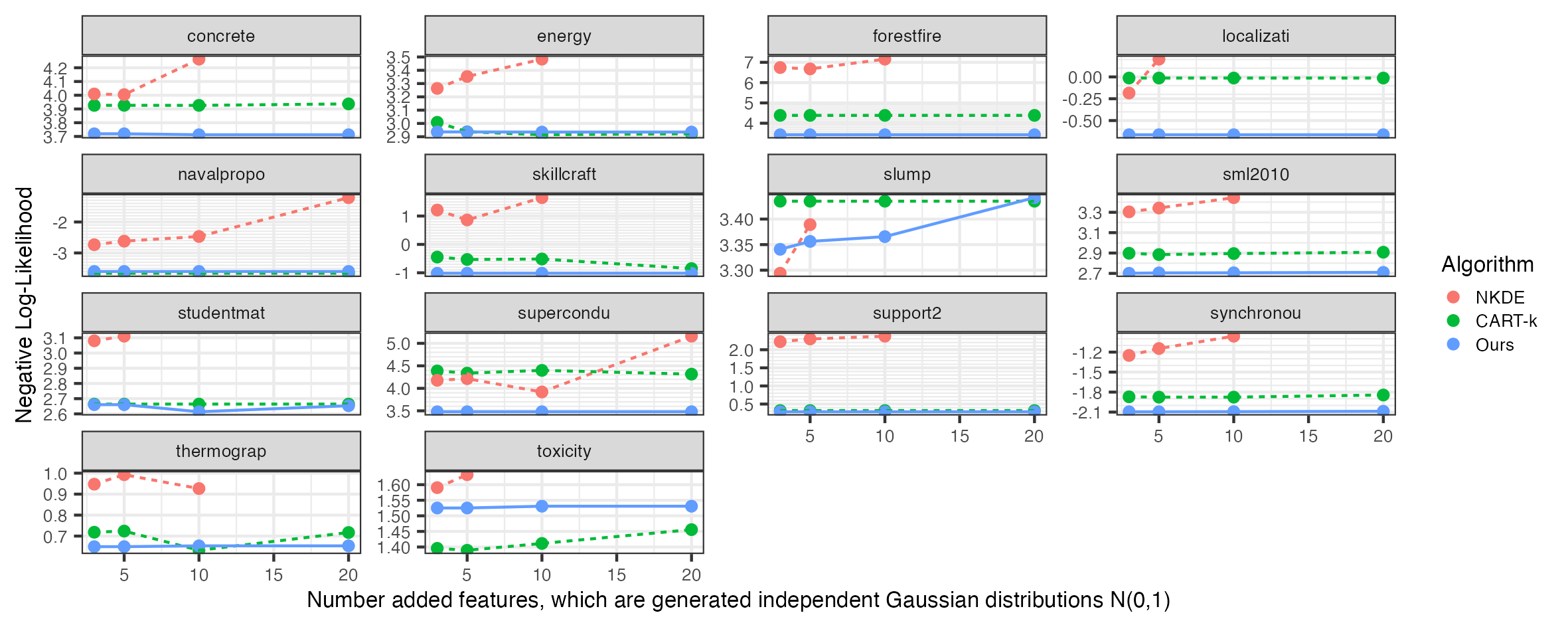
Figure 5: Negative-log-likelihoods with different number of added features, which are generated by independent Gaussian distributions. The results of CDTree, shown in blue solid lines, are extremely stable on all datasets expect for the very small ‘slump’ dataset.

Appendix E Medical costs visualizations

We show in Figure 6 the full results of applying CDTree to the medical expenses dataset used in Section 1. As a sanity check for the goodness-of-fit, we report the average cross-validation negative log-likelihood (on test sets) for CDTree is $9.03$ (with the standard deviation $0.13$), which is slightly better than that of the black-box boosted tree model LinCDE, with the average negative log-likelihood $9.55$ (standard deviation $0.09$). Each Histogram corresponds to a single leaf that describes a meaningful subgroup of patients, in which we observe ‘age’, ‘BMI’, and ‘smoker’ are the most distinguishing features to characterize each subgroup. Last, although the dataset contains 9 features and only 1338 samples, the illustrations show that CDTree does not require a very large dataset to reveal meaningful and comprehensible information.

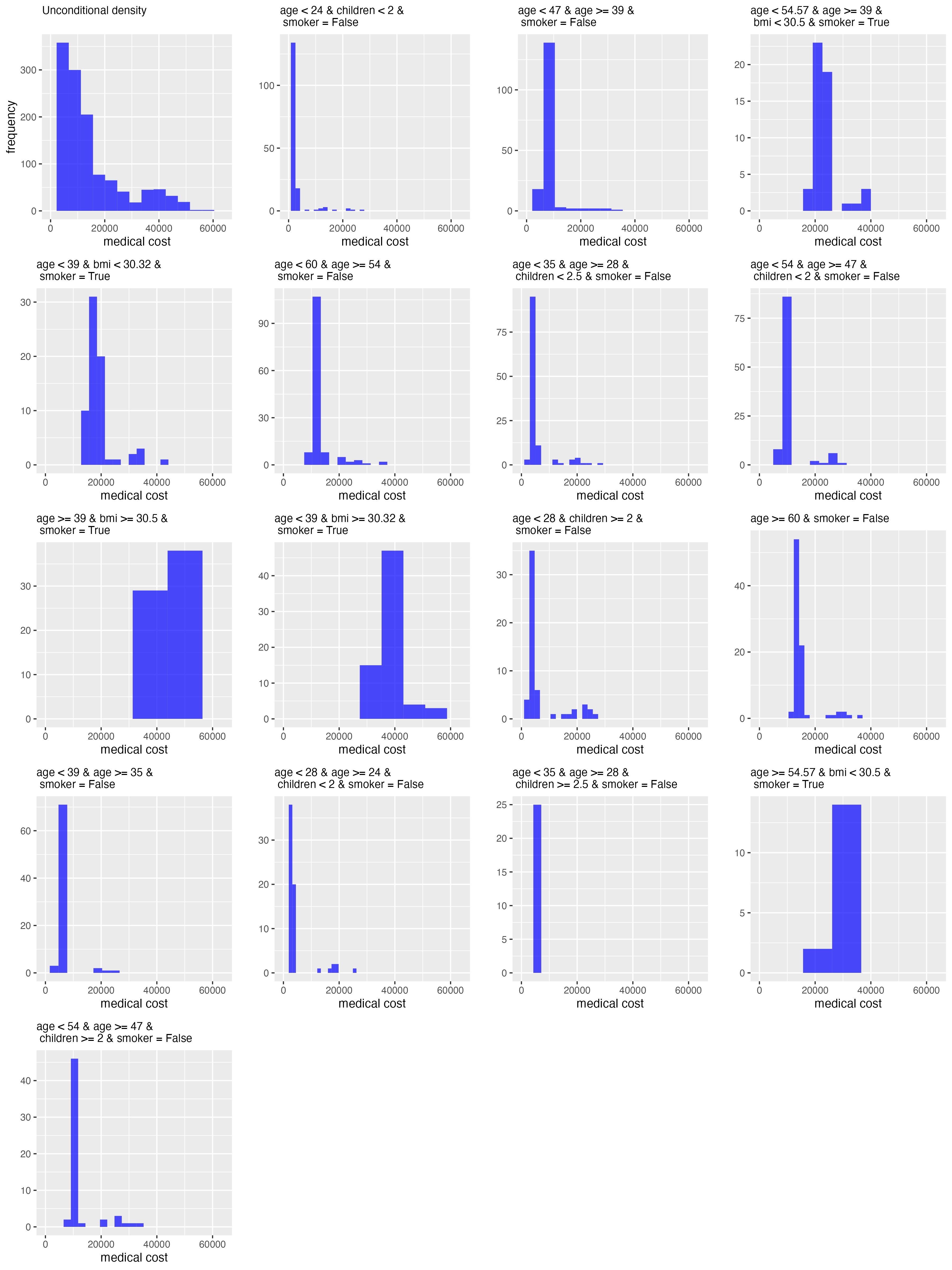
Figure 6: All leaves from the CDTree that describes the conditional density of medical costs, conditioned on demographic features. Root-to-leaf conditions are presented after removing logically redundant conditions.

NeurIPS Paper Checklist

The checklist is designed to encourage best practices for responsible machine learning research, addressing issues of reproducibility, transparency, research ethics, and societal impact. Do not remove the checklist: The papers not including the checklist will be desk rejected. The checklist should follow the references and follow the (optional) supplemental material. The checklist does NOT count towards the page limit.

Please read the checklist guidelines carefully for information on how to answer these questions. For each question in the checklist:

• You should answer [Yes] , [No] , or [N/A] .

• [N/A] means either that the question is Not Applicable for that particular paper or the relevant information is Not Available.

• Please provide a short (1–2 sentence) justification right after your answer (even for NA).

The checklist answers are an integral part of your paper submission. They are visible to the reviewers, area chairs, senior area chairs, and ethics reviewers. You will be asked to also include it (after eventual revisions) with the final version of your paper, and its final version will be published with the paper.

The reviewers of your paper will be asked to use the checklist as one of the factors in their evaluation. While "[Yes] " is generally preferable to "[No] ", it is perfectly acceptable to answer "[No] " provided a proper justification is given (e.g., "error bars are not reported because it would be too computationally expensive" or "we were unable to find the license for the dataset we used"). In general, answering "[No] " or "[N/A] " is not grounds for rejection. While the questions are phrased in a binary way, we acknowledge that the true answer is often more nuanced, so please just use your best judgment and write a justification to elaborate. All supporting evidence can appear either in the main paper or the supplemental material, provided in appendix. If you answer [Yes] to a question, in the justification please point to the section(s) where related material for the question can be found.

1. Claims

2. Question: Do the main claims made in the abstract and introduction accurately reflect the paper’s contributions and scope?

3. Answer: [Yes]

4. Justification: Our mains claims and the paper’s contributions are both 1) to introduce a tree-based CDE method, and 2) we show that our proposed method is both more accurate (as measured by the log-loss), has smaller tree sizes, and is robust against irrelevant features.

5. Guidelines:

   • The answer NA means that the abstract and introduction do not include the claims made in the paper.

   • The abstract and/or introduction should clearly state the claims made, including the contributions made in the paper and important assumptions and limitations. A No or NA answer to this question will not be perceived well by the reviewers.

   • The claims made should match theoretical and experimental results, and reflect how much the results can be expected to generalize to other settings.

   • It is fine to include aspirational goals as motivation as long as it is clear that these goals are not attained by the paper.

6. Limitations

7. Question: Does the paper discuss the limitations of the work performed by the authors?

8. Answer: [Yes]

9. Justification: We have a separate ‘limitation’ subsection within the Discussion Section in Section 7.

10. Guidelines:

    • The answer NA means that the paper has no limitation while the answer No means that the paper has limitations, but those are not discussed in the paper.

    • The authors are encouraged to create a separate "Limitations" section in their paper.

    • The paper should point out any strong assumptions and how robust the results are to violations of these assumptions (e.g., independence assumptions, noiseless settings, model well-specification, asymptotic approximations only holding locally). The authors should reflect on how these assumptions might be violated in practice and what the implications would be.

    • The authors should reflect on the scope of the claims made, e.g., if the approach was only tested on a few datasets or with a few runs. In general, empirical results often depend on implicit assumptions, which should be articulated.

    • The authors should reflect on the factors that influence the performance of the approach. For example, a facial recognition algorithm may perform poorly when image resolution is low or images are taken in low lighting. Or a speech-to-text system might not be used reliably to provide closed captions for online lectures because it fails to handle technical jargon.

    • The authors should discuss the computational efficiency of the proposed algorithms and how they scale with dataset size.

    • If applicable, the authors should discuss possible limitations of their approach to address problems of privacy and fairness.

    • While the authors might fear that complete honesty about limitations might be used by reviewers as grounds for rejection, a worse outcome might be that reviewers discover limitations that aren’t acknowledged in the paper. The authors should use their best judgment and recognize that individual actions in favor of transparency play an important role in developing norms that preserve the integrity of the community. Reviewers will be specifically instructed to not penalize honesty concerning limitations.

11. Theory Assumptions and Proofs

12. Question: For each theoretical result, does the paper provide the full set of assumptions and a complete (and correct) proof?

13. Answer: [Yes]

14. Justification: our proof has no additional assumptions.

15. Guidelines:

    • The answer NA means that the paper does not include theoretical results.

    • All the theorems, formulas, and proofs in the paper should be numbered and cross-referenced.

    • All assumptions should be clearly stated or referenced in the statement of any theorems.

    • The proofs can either appear in the main paper or the supplemental material, but if they appear in the supplemental material, the authors are encouraged to provide a short proof sketch to provide intuition.

    • Inversely, any informal proof provided in the core of the paper should be complemented by formal proofs provided in appendix or supplemental material.

    • Theorems and Lemmas that the proof relies upon should be properly referenced.

16. Experimental Result Reproducibility

17. Question: Does the paper fully disclose all the information needed to reproduce the main experimental results of the paper to the extent that it affects the main claims and/or conclusions of the paper (regardless of whether the code and data are provided or not)?

18. Answer: [Yes]

19. Justification: Full descriptions are provided both in the main context and in the appendix. Also, the source code is provided.

20. Guidelines:

    • The answer NA means that the paper does not include experiments.

    • If the paper includes experiments, a No answer to this question will not be perceived well by the reviewers: Making the paper reproducible is important, regardless of whether the code and data are provided or not.

    • If the contribution is a dataset and/or model, the authors should describe the steps taken to make their results reproducible or verifiable.

    • Depending on the contribution, reproducibility can be accomplished in various ways. For example, if the contribution is a novel architecture, describing the architecture fully might suffice, or if the contribution is a specific model and empirical evaluation, it may be necessary to either make it possible for others to replicate the model with the same dataset, or provide access to the model. In general. releasing code and data is often one good way to accomplish this, but reproducibility can also be provided via detailed instructions for how to replicate the results, access to a hosted model (e.g., in the case of a large language model), releasing of a model checkpoint, or other means that are appropriate to the research performed.

    • While NeurIPS does not require releasing code, the conference does require all submissions to provide some reasonable avenue for reproducibility, which may depend on the nature of the contribution. For example

      1. If the contribution is primarily a new algorithm, the paper should make it clear how to reproduce that algorithm.

      2. If the contribution is primarily a new model architecture, the paper should describe the architecture clearly and fully.

      3. If the contribution is a new model (e.g., a large language model), then there should either be a way to access this model for reproducing the results or a way to reproduce the model (e.g., with an open-source dataset or instructions for how to construct the dataset).

      4. We recognize that reproducibility may be tricky in some cases, in which case authors are welcome to describe the particular way they provide for reproducibility. In the case of closed-source models, it may be that access to the model is limited in some way (e.g., to registered users), but it should be possible for other researchers to have some path to reproducing or verifying the results.

21. Open access to data and code

22. Question: Does the paper provide open access to the data and code, with sufficient instructions to faithfully reproduce the main experimental results, as described in supplemental material?

23. Answer: [Yes]

24. Justification: The source code is provided. The datasets are all available on the website of the UCI repository.

25. Guidelines:

    • The answer NA means that paper does not include experiments requiring code.

    • Please see the NeurIPS code and data submission guidelines (https://nips.cc/public/guides/CodeSubmissionPolicy) for more details.

    • While we encourage the release of code and data, we understand that this might not be possible, so “No” is an acceptable answer. Papers cannot be rejected simply for not including code, unless this is central to the contribution (e.g., for a new open-source benchmark).

    • The instructions should contain the exact command and environment needed to run to reproduce the results. See the NeurIPS code and data submission guidelines (https://nips.cc/public/guides/CodeSubmissionPolicy) for more details.

    • The authors should provide instructions on data access and preparation, including how to access the raw data, preprocessed data, intermediate data, and generated data, etc.

    • The authors should provide scripts to reproduce all experimental results for the new proposed method and baselines. If only a subset of experiments are reproducible, they should state which ones are omitted from the script and why.

    • At submission time, to preserve anonymity, the authors should release anonymized versions (if applicable).

    • Providing as much information as possible in supplemental material (appended to the paper) is recommended, but including URLs to data and code is permitted.

26. Experimental Setting/Details

27. Question: Does the paper specify all the training and test details (e.g., data splits, hyperparameters, how they were chosen, type of optimizer, etc.) necessary to understand the results?

28. Answer: [Yes]

29. Justification: Full descriptions are provided both in the main context and in the appendix.

30. Guidelines:

    • The answer NA means that the paper does not include experiments.

    • The experimental setting should be presented in the core of the paper to a level of detail that is necessary to appreciate the results and make sense of them.

    • The full details can be provided either with the code, in appendix, or as supplemental material.

31. Experiment Statistical Significance

32. Question: Does the paper report error bars suitably and correctly defined or other appropriate information about the statistical significance of the experiments?

33. Answer: [Yes]

34. Justification: we report the standard deviation of the negative log-likelihoods, obtained by five-fold cross-validation, in Appendix D.1.

35. Guidelines:

    • The answer NA means that the paper does not include experiments.

    • The authors should answer "Yes" if the results are accompanied by error bars, confidence intervals, or statistical significance tests, at least for the experiments that support the main claims of the paper.

    • The factors of variability that the error bars are capturing should be clearly stated (for example, train/test split, initialization, random drawing of some parameter, or overall run with given experimental conditions).

    • The method for calculating the error bars should be explained (closed form formula, call to a library function, bootstrap, etc.)

    • The assumptions made should be given (e.g., Normally distributed errors).

    • It should be clear whether the error bar is the standard deviation or the standard error of the mean.

    • It is OK to report 1-sigma error bars, but one should state it. The authors should preferably report a 2-sigma error bar than state that they have a 96% CI, if the hypothesis of Normality of errors is not verified.

    • For asymmetric distributions, the authors should be careful not to show in tables or figures symmetric error bars that would yield results that are out of range (e.g. negative error rates).

    • If error bars are reported in tables or plots, The authors should explain in the text how they were calculated and reference the corresponding figures or tables in the text.

36. Experiments Compute Resources

37. Question: For each experiment, does the paper provide sufficient information on the computer resources (type of compute workers, memory, time of execution) needed to reproduce the experiments?

38. Answer: [Yes]

39. Justification: We report the compute resources in Appendix C.1.

40. Guidelines:

    • The answer NA means that the paper does not include experiments.

    • The paper should indicate the type of compute workers CPU or GPU, internal cluster, or cloud provider, including relevant memory and storage.

    • The paper should provide the amount of compute required for each of the individual experimental runs as well as estimate the total compute.

    • The paper should disclose whether the full research project required more compute than the experiments reported in the paper (e.g., preliminary or failed experiments that didn’t make it into the paper).

41. Code Of Ethics

42. Question: Does the research conducted in the paper conform, in every respect, with the NeurIPS Code of Ethics https://neurips.cc/public/EthicsGuidelines?

43. Answer: [Yes]

44. Justification: [N/A]

45. Guidelines:

    • The answer NA means that the authors have not reviewed the NeurIPS Code of Ethics.

    • If the authors answer No, they should explain the special circumstances that require a deviation from the Code of Ethics.

    • The authors should make sure to preserve anonymity (e.g., if there is a special consideration due to laws or regulations in their jurisdiction).

46. Broader Impacts

47. Question: Does the paper discuss both potential positive societal impacts and negative societal impacts of the work performed?

48. Answer: [Yes]

49. Justification: The paper discusses the positive societal impacts about 1) interpretable CDE methods have advantages in critical domains, 2) CDTree is more interpretable than kernel-based methods because it is also interpretable to the general public without Statistics knowledge. As far as we are concerned, our method does not have the risk of being misused in a malicious way.

50. Guidelines:

    • The answer NA means that there is no societal impact of the work performed.

    • If the authors answer NA or No, they should explain why their work has no societal impact or why the paper does not address societal impact.

    • Examples of negative societal impacts include potential malicious or unintended uses (e.g., disinformation, generating fake profiles, surveillance), fairness considerations (e.g., deployment of technologies that could make decisions that unfairly impact specific groups), privacy considerations, and security considerations.

    • The conference expects that many papers will be foundational research and not tied to particular applications, let alone deployments. However, if there is a direct path to any negative applications, the authors should point it out. For example, it is legitimate to point out that an improvement in the quality of generative models could be used to generate deepfakes for disinformation. On the other hand, it is not needed to point out that a generic algorithm for optimizing neural networks could enable people to train models that generate Deepfakes faster.

    • The authors should consider possible harms that could arise when the technology is being used as intended and functioning correctly, harms that could arise when the technology is being used as intended but gives incorrect results, and harms following from (intentional or unintentional) misuse of the technology.

    • If there are negative societal impacts, the authors could also discuss possible mitigation strategies (e.g., gated release of models, providing defenses in addition to attacks, mechanisms for monitoring misuse, mechanisms to monitor how a system learns from feedback over time, improving the efficiency and accessibility of ML).

51. Safeguards

52. Question: Does the paper describe safeguards that have been put in place for responsible release of data or models that have a high risk for misuse (e.g., pretrained language models, image generators, or scraped datasets)?

53. Answer: [N/A]

54. Justification: [N/A]

55. Guidelines:

    • The answer NA means that the paper poses no such risks.

    • Released models that have a high risk for misuse or dual-use should be released with necessary safeguards to allow for controlled use of the model, for example by requiring that users adhere to usage guidelines or restrictions to access the model or implementing safety filters.

    • Datasets that have been scraped from the Internet could pose safety risks. The authors should describe how they avoided releasing unsafe images.

    • We recognize that providing effective safeguards is challenging, and many papers do not require this, but we encourage authors to take this into account and make a best faith effort.

56. Licenses for existing assets

57. Question: Are the creators or original owners of assets (e.g., code, data, models), used in the paper, properly credited and are the license and terms of use explicitly mentioned and properly respected?

58. Answer: [Yes]

59. Justification: All datasets and code are free to use for research purposes according to the licenses.

60. Guidelines:

    • The answer NA means that the paper does not use existing assets.

    • The authors should cite the original paper that produced the code package or dataset.

    • The authors should state which version of the asset is used and, if possible, include a URL.

    • The name of the license (e.g., CC-BY 4.0) should be included for each asset.

    • For scraped data from a particular source (e.g., website), the copyright and terms of service of that source should be provided.

    • If assets are released, the license, copyright information, and terms of use in the package should be provided. For popular datasets, paperswithcode.com/datasets has curated licenses for some datasets. Their licensing guide can help determine the license of a dataset.

    • For existing datasets that are re-packaged, both the original license and the license of the derived asset (if it has changed) should be provided.

    • If this information is not available online, the authors are encouraged to reach out to the asset’s creators.

61. New Assets

62. Question: Are new assets introduced in the paper well documented and is the documentation provided alongside the assets?

63. Answer: [Yes]

64. Justification: Source code is provided, together with the details of how to get the code running.

65. Guidelines:

    • The answer NA means that the paper does not release new assets.

    • Researchers should communicate the details of the dataset/code/model as part of their submissions via structured templates. This includes details about training, license, limitations, etc.

    • The paper should discuss whether and how consent was obtained from people whose asset is used.

    • At submission time, remember to anonymize your assets (if applicable). You can either create an anonymized URL or include an anonymized zip file.

66. Crowdsourcing and Research with Human Subjects

67. Question: For crowdsourcing experiments and research with human subjects, does the paper include the full text of instructions given to participants and screenshots, if applicable, as well as details about compensation (if any)?

68. Answer: [N/A]

69. Justification: [N/A]

70. Guidelines:

    • The answer NA means that the paper does not involve crowdsourcing nor research with human subjects.

    • Including this information in the supplemental material is fine, but if the main contribution of the paper involves human subjects, then as much detail as possible should be included in the main paper.

    • According to the NeurIPS Code of Ethics, workers involved in data collection, curation, or other labor should be paid at least the minimum wage in the country of the data collector.

71. Institutional Review Board (IRB) Approvals or Equivalent for Research with Human Subjects

72. Question: Does the paper describe potential risks incurred by study participants, whether such risks were disclosed to the subjects, and whether Institutional Review Board (IRB) approvals (or an equivalent approval/review based on the requirements of your country or institution) were obtained?

73. Answer: [N/A]

74. Justification: [N/A]

75. Guidelines:

    • The answer NA means that the paper does not involve crowdsourcing nor research with human subjects.

    • Depending on the country in which research is conducted, IRB approval (or equivalent) may be required for any human subjects research. If you obtained IRB approval, you should clearly state this in the paper.

    • We recognize that the procedures for this may vary significantly between institutions and locations, and we expect authors to adhere to the NeurIPS Code of Ethics and the guidelines for their institution.

    • For initial submissions, do not include any information that would break anonymity (if applicable), such as the institution conducting the review.

References

- [1] The uci machine learning repository. URL https://archive.ics.uci.edu/.
- Athreya et al. [2004] K. B. Athreya, P. E. Ney, and P. Ney. Branching processes. Courier Corporation, 2004.
- Ball et al. [2008] N. M. Ball, R. J. Brunner, A. D. Myers, N. E. Strand, S. L. Alberts, and D. Tcheng. Robust machine learning applied to astronomical data sets. iii. probabilistic photometric redshifts for galaxies and quasars in the sdss and galex. The Astrophysical Journal, 683(1):12, 2008.
- Bishop [1994] C. M. Bishop. Mixture density networks. 1994.
- Breiman [2017] L. Breiman. Classification and regression trees. Routledge, 2017.
- Cousins and Riondato [2019] C. Cousins and M. Riondato. Cadet: interpretable parametric conditional density estimation with decision trees and forests. Machine Learning, 108:1613–1634, 2019.
- Cover and Thomas [2012] T. M. Cover and J. A. Thomas. Elements of information theory. John Wiley & Sons, 2012.
- DeSantis et al. [2014] C. DeSantis, J. Ma, L. Bryan, and A. Jemal. Breast cancer statistics, 2013. CA: a cancer journal for clinicians, 64(1):52–62, 2014.
- Durrieu et al. [2018] G. Durrieu, I. Grama, K. Jaunatre, Q.-K. Pham, and J.-M. Tricot. Extremefit: a package for extreme quantiles. Journal of Statistical Software, 87:1–20, 2018.
- Dutordoir et al. [2018] V. Dutordoir, H. Salimbeni, J. Hensman, and M. Deisenroth. Gaussian process conditional density estimation. Advances in neural information processing systems, 31, 2018.
- Fan et al. [1996] J. Fan, Q. Yao, and H. Tong. Estimation of conditional densities and sensitivity measures in nonlinear dynamical systems. Biometrika, 83(1):189–206, 1996.
- Galbrun [2022] E. Galbrun. The minimum description length principle for pattern mining: A survey. Data mining and knowledge discovery, 36(5):1679–1727, 2022.
- Gao and Hastie [2022] Z. Gao and T. Hastie. Lincde: conditional density estimation via lindsey’s method. Journal of machine learning research, 23(52):1–55, 2022.
- Gilleskie and Mroz [2004] D. B. Gilleskie and T. A. Mroz. A flexible approach for estimating the effects of covariates on health expenditures. Journal of health economics, 23(2):391–418, 2004.
- Grünwald [2007] P. Grünwald. The minimum description length principle. MIT press, 2007.
- Grünwald and Roos [2019] P. Grünwald and T. Roos. Minimum description length revisited. arXiv preprint arXiv:1908.08484, 2019.
- Hall et al. [2004] P. Hall, J. Racine, and Q. Li. Cross-validation and the estimation of conditional probability densities. Journal of the American Statistical Association, 99(468):1015–1026, 2004.
- Hu et al. [2019] X. Hu, C. Rudin, and M. Seltzer. Optimal sparse decision trees. Advances in Neural Information Processing Systems, 32, 2019.
- Jeon and Taylor [2012] J. Jeon and J. W. Taylor. Using conditional kernel density estimation for wind power density forecasting. Journal of the American Statistical Association, 107(497):66–79, 2012.
- Kontkanen and Myllymäki [2005] P. Kontkanen and P. Myllymäki. Analyzing the stochastic complexity via tree polynomials. Unpublished manuscript, 2005.
- Kontkanen and Myllymäki [2007a] P. Kontkanen and P. Myllymäki. A linear-time algorithm for computing the multinomial stochastic complexity. Information Processing Letters, 103(6):227–233, 2007a.
- Kontkanen and Myllymäki [2007b] P. Kontkanen and P. Myllymäki. MDL histogram density estimation. In M. Meila and X. Shen, editors, Proceedings of the Eleventh International Conference on Artificial Intelligence and Statistics, volume 2 of Proceedings of Machine Learning Research. PMLR, 2007b.
- Kotz and Nadarajah [2000] S. Kotz and S. Nadarajah. Extreme value distributions: theory and applications. world scientific, 2000.
- Lantz [2019] B. Lantz. Machine learning with R: expert techniques for predictive modeling. Packt publishing ltd, 2019.
- Lindsey [1974] J. Lindsey. Comparison of probability distributions. Journal of the Royal Statistical Society: Series B (Methodological), 36(1):38–47, 1974.
- Luo and Khoshgoftaar [2006] Q. Luo and T. M. Khoshgoftaar. Unsupervised multiscale color image segmentation based on mdl principle. IEEE Transactions on Image Processing, 15(9):2755–2761, 2006.
- Malerba et al. [2004] D. Malerba, F. Esposito, M. Ceci, and A. Appice. Top-down induction of model trees with regression and splitting nodes. IEEE Transactions on Pattern Analysis and Machine Intelligence, 26(5):612–625, 2004.
- Marx et al. [2021] A. Marx, L. Yang, and M. van Leeuwen. Estimating conditional mutual information for discrete-continuous mixtures using multi-dimensional adaptive histograms. In Proceedings of the 2021 SIAM International Conference on Data Mining (SDM), pages 387–395. SIAM, 2021.
- Molnar [2020] C. Molnar. Interpretable machine learning. Lulu.com, 2020.
- Mononen and Myllymäki [2008] T. Mononen and P. Myllymäki. Computing the multinomial stochastic complexity in sub-linear time. In Proceedings of the 4th European Workshop on Probabilistic Graphical Models, pages 209–216, 2008.
- Mussa [2013] H. Y. Mussa. The aitchison and aitken kernel function revisited. Journal of Mathematics Research, 5(1):22, 2013.
- Nikolova et al. [2012] S. Nikolova, A. Sinko, and M. Sutton. Do maximum waiting times guarantees change clinical priorities? a conditional density estimation approach. Technical report, HEDG, c/o Department of Economics, University of York, 2012.
- Papageorgiou and Kontoyiannis [2024] I. Papageorgiou and I. Kontoyiannis. Posterior representations for bayesian context trees: Sampling, estimation and convergence. Bayesian analysis, 19(2):501–529, 2024.
- Pedregosa et al. [2011] F. Pedregosa, G. Varoquaux, A. Gramfort, V. Michel, B. Thirion, O. Grisel, M. Blondel, P. Prettenhofer, R. Weiss, V. Dubourg, J. Vanderplas, A. Passos, D. Cournapeau, M. Brucher, M. Perrot, and E. Duchesnay. Scikit-learn: Machine learning in Python. Journal of Machine Learning Research, 12:2825–2830, 2011.
- Pospisil and Lee [2018] T. Pospisil and A. B. Lee. Rfcde: Random forests for conditional density estimation. arXiv preprint arXiv:1804.05753, 2018.
- Proença and van Leeuwen [2020] H. M. Proença and M. van Leeuwen. Interpretable multiclass classification by mdl-based rule lists. Information Sciences, 512:1372–1393, 2020.
- Quinlan [2014] J. R. Quinlan. C4. 5: programs for machine learning. Elsevier, 2014.
- Quinlan et al. [1992] J. R. Quinlan et al. Learning with continuous classes. In 5th Australian joint conference on artificial intelligence, volume 92, pages 343–348. World Scientific, 1992.
- Rezende and Mohamed [2015] D. Rezende and S. Mohamed. Variational inference with normalizing flows. In International conference on machine learning, pages 1530–1538. PMLR, 2015.
- Ribeiro et al. [2016] M. T. Ribeiro, S. Singh, and C. Guestrin. Why should i trust you? explaining the predictions of any classifier. In Proceedings of the 22nd ACM SIGKDD international conference on knowledge discovery and data mining, pages 1135–1144, 2016.
- Rissanen [1978] J. Rissanen. Modeling by shortest data description. Automatica, 14(5):465–471, 1978.
- Rissanen [1983] J. Rissanen. A universal prior for integers and estimation by minimum description length. The Annals of statistics, 11(2):416–431, 1983.
- Roos et al. [2008] T. Roos, T. Silander, P. Kontkanen, and P. Myllymaki. Bayesian network structure learning using factorized nml universal models. In 2008 Information Theory and Applications Workshop, pages 272–276. IEEE, 2008.
- Rosenblatt [1969] M. Rosenblatt. Conditional probability density and regression estimators. Multivariate analysis II, 25:31, 1969.
- Rothfuss et al. [2019a] J. Rothfuss, F. Ferreira, S. Boehm, S. Walther, M. Ulrich, T. Asfour, and A. Krause. Noise regularization for conditional density estimation. arXiv:1907.08982, 2019a.
- Rothfuss et al. [2019b] J. Rothfuss, F. Ferreira, S. Walther, and M. Ulrich. Conditional density estimation with neural networks: Best practices and benchmarks. arXiv preprint arXiv:1903.00954, 2019b.
- Samani et al. [2021] F. S. Samani, R. Stadler, C. Flinta, and A. Johnsson. Conditional density estimation of service metrics for networked services. IEEE Transactions on Network and Service Management, 18(2):2350–2364, 2021.
- Seabold and Perktold [2010] S. Seabold and J. Perktold. statsmodels: Econometric and statistical modeling with python. In 9th Python in Science Conference, 2010.
- Shtar’kov [1987] Y. M. Shtar’kov. Universal sequential coding of single messages. Problemy Peredachi Informatsii, 23(3):3–17, 1987.
- Shu et al. [2017] R. Shu, H. H. Bui, and M. Ghavamzadeh. Bottleneck conditional density estimation. In International conference on machine learning, pages 3164–3172. PMLR, 2017.
- Silander et al. [2018] T. Silander, J. Leppä-Aho, E. Jääsaari, and T. Roos. Quotient normalized maximum likelihood criterion for learning bayesian network structures. In International conference on artificial intelligence and statistics, pages 948–957. PMLR, 2018.
- Stanley [2015] R. P. Stanley. Catalan numbers. Cambridge University Press, 2015.
- Strobl and Visweswaran [2021] E. V. Strobl and S. Visweswaran. Dirac delta regression: Conditional density estimation with clinical trials. In The KDD’21 Workshop on Causal Discovery, pages 78–125. PMLR, 2021.
- Sugiyama et al. [2010] M. Sugiyama, I. Takeuchi, T. Suzuki, T. Kanamori, H. Hachiya, and D. Okanohara. Conditional density estimation via least-squares density ratio estimation. In Proceedings of the Thirteenth International Conference on Artificial Intelligence and Statistics, pages 781–788. JMLR Workshop and Conference Proceedings, 2010.
- Trippe and Turner [2018] B. L. Trippe and R. E. Turner. Conditional density estimation with bayesian normalising flows. arXiv preprint arXiv:1802.04908, 2018.
- Virtanen et al. [2020] P. Virtanen, R. Gommers, T. E. Oliphant, M. Haberland, T. Reddy, D. Cournapeau, E. Burovski, P. Peterson, W. Weckesser, J. Bright, S. J. van der Walt, M. Brett, J. Wilson, K. J. Millman, N. Mayorov, A. R. J. Nelson, E. Jones, R. Kern, E. Larson, C. J. Carey, İ. Polat, Y. Feng, E. W. Moore, J. VanderPlas, D. Laxalde, J. Perktold, R. Cimrman, I. Henriksen, E. A. Quintero, C. R. Harris, A. M. Archibald, A. H. Ribeiro, F. Pedregosa, P. van Mulbregt, and SciPy 1.0 Contributors. SciPy 1.0: Fundamental Algorithms for Scientific Computing in Python. Nature Methods, 17:261–272, 2020. doi: 10.1038/s41592-019-0686-2.
- Yang and van Leeuwen [2022] L. Yang and M. van Leeuwen. Truly unordered probabilistic rule sets for multi-class classification. In Joint European Conference on Machine Learning and Knowledge Discovery in Databases, pages 87–103. Springer, 2022.
- Yang et al. [2023] L. Yang, M. Baratchi, and M. van Leeuwen. Unsupervised discretization by two-dimensional mdl-based histogram. Machine Learning, pages 1–35, 2023.
- Zhang et al. [2023] R. Zhang, R. Xin, M. Seltzer, and C. Rudin. Optimal sparse regression trees. In Proceedings of the AAAI Conference on Artificial Intelligence, volume 37, pages 11270–11279, 2023.