On Championing Foundation Models: From Explainability to Interpretability
Abstract
Understanding the inner mechanisms of black-box foundation models (FMs) is essential yet challenging in artificial intelligence and its applications. Over the last decade, the long-running focus has been on their explainability, leading to the development of post-hoc explainable methods to rationalize the specific decisions already made by black-box FMs. However, these explainable methods have certain limitations in terms of faithfulness, detail capture and resource requirement. Consequently, in response to these issues, a new class of interpretable methods should be considered to unveil the underlying mechanisms in an accurate, comprehensive, heuristic and resource-light way. This survey aims to review interpretable methods that comply with the aforementioned principles and have been successfully applied to FMs. These methods are deeply rooted in machine learning theory, covering the analysis of generalization performance, expressive capability, and dynamic behavior. They provide a thorough interpretation of the entire workflow of FMs, ranging from the inference capability and training dynamics to their ethical implications. Ultimately, drawing upon these interpretations, this review identifies the next frontier research directions for FMs.
Keywords: Foundation models; explainable method; interpretable methods; machine learning theory
1 Introduction
Foundation Models (FMs), emerging as a new paradigm in deep learning, are fundamentally changing the landscape of artificial intelligence (AI). Unlike traditional models trained for specific tasks, FMs leverage massive and diverse datasets for training, which allows them to handle various downstream tasks through techniques like supervised fine-tuning (SFT) [1], Reinforcement Learning from Human Feedback (RLHF) [2], Retrieval Augmented Generation (RAG) [3], prompting engineering [4, 5] or continual learning [6]. In natural language processing, most FMs under autoregressive structure (e.g., GPT-3 [7], PaLM [8], or Chinchilla [9]) are established to output the next token given a sequence. Most text-to-image models, for example DALL·E [10], are trained to capture the distribution of images given a text input. Video FMs, trained on video data, potentially combined with text or audio, can be categorized based on their pretraining goals: generative models like VideoBERT [11] focus on creating new video content, while discriminative models like VideoCLIP [12] excel at recognizing and classifying video elements. Hybrid approaches like TVLT [13] combine these strengths for more versatile tasks. FMs have the potential to revolutionize a vast array of industries. Consider ChatGPT, a versatile chatbot developed by OpenAI, which has already made strides in enhancing customer support, virtual assistants, and voice-activated devices [14]. As FMs become more integrated into various products, their deployments will be scaled to accommodate a growing user base. This trend is evident in the growing list of companies, such as Microsoft with Bing Chat and Google with Bard, all planning to deploy similar FMs-powered products, further expanding the reach of this technology.
1.1 The Bottleneck of Explainability in Foundation Models
Despite of rapid development of FMs, there are also ongoing concerns that continue to arise. The underlying causes behind certain emerging properties in FMs remain unclear. [15] firstly consider a focused definition of emergent abilities of FMs: “an ability is emergent if it is not present in smaller models but is present in larger models”. They conduct sufficient empirical studies to show emergent abilities can span a variety of large-scale language models, task types, and experimental scenarios. On the contrary, serveral works claim that emergent abilities only appear for specific metrics, not for model families on particular tasks, and that changing the metric causes the emergence phenomenon to disappear [16]. Moreover, prompting strategies can elicit chains of thought (CoT), suggesting a potential for reasoning abilities of FMs [5]. However, recent critiques by Arkoudas highlight limitations in current evaluation methods, arguing that GPT-4’s occasional displays of analytical prowess may not translate to true reasoning capabilities [17]. ‘All that glitters is not gold’, as potential risks gradually emerge behind the prosperous phenomenon. The phenomenon of “hallucination” has garnered widespread public attention, referring to the tendency of FMs to generate text that sounds convincing, even if it is fabricated or misleading, as discussed in recent research [18]. Additionally, studies have shown that adding a series of specific meaningless tokens can lead to security failures, resulting in the unlimited leakage of sensitive content [19]. These issues serve as stark reminders that we still lack a comprehensive understanding of the intricate workings of FMs, hindering our ability to fully unleash their potential while mitigating potential risks.
The term “explainability” refers to the ability to understand the decision-making process of an AI model. Specifically, most explainable methods concentrates on providing users with post-hoc explanations on the specific decisions already made by the black-box models [20, 21, 22]. Recently, several survey studies review local and global explainable methods for FMs [21, 22, 23]. Local methods, like feature attribution [24, 25, 26], attention-based explanation [27, 28, 29], and example-based explanation [30, 31], focus on understanding the model’s decisions for specific instances. Conversely, global methods, such as probing-based explanation [32, 33], neuron activation explanation [34, 35], and mechanistic explanation [36, 37], aim to delve into the broader picture, revealing what input variables significantly influence the model as a whole. More specifically, these explanation techniques demonstrate excellent performance in exploring the differences in how humans and FMs work. For instance, [38] utilize perturbation based explainable approach, SHAP (SHapley Additive exPlanations) [25], to investigate the influence of code tokens on summary generation, and find no evidence of a statistically significant relationship between attention mechanisms in FMs and human programmers. Endeavors are also being made to propose explainable methods tailored specifically for FMs. [39] propose a novel framework to provide impact-aware explanations, which are robust to feature changes and influential to the model’s predictions. Recently, a GPT-4 based explainable method is utilized to explain the behavior of neurons in GPT-2 [34].
However, explanations garnered from these explanable methods for complex FMs are often not entirely reliable and may even be misleading:
-
•
Inherent Unfaithfullness: [20] argue that if an explanation perfectly mirrored the model’s computations, the explanation itself would suffice, rendering the original model unnecessary. This highlights a key limitation of explainable methods for complex models: any explanation technique applied to a black-box model is likely to be an inaccurate representation. For instance, adversarial examples are carefully crafted inputs that are slightly perturbed from the original data, but often lead to misclassification or incorrect predictions by deep learning models. When using explainable methods to analyze and provide explanations for the model’s decisions on adversarial examples, the explanations may fail to capture the true underlying reasons for the misclassification.
-
•
Insufficient Detail: Even in a scenario where both the FMs and their explanation method are accurate – the models’ prediction is correct, and the explanation faithfully approximates it – the explanation might still be so devoid of detail as to be meaningless. For instance, consider an image of a dog with a frisbee in its mouth. An AI model can recognize it as a dog, but the explainable method might highlight only the dog’s overall shape or a few prominent features. The explanation may not reveal why the model made the correct prediction or the specific cues it used to recognize the dog.
-
•
Shallow Understanding: Current explainable methods primarily focus on addressing the crucial question of “how does the model achieve its output?", e.g., identifying which features play a significant role in decision-making. However, these methods often struggle to answer the fundamental questions that are particularly relevant to FMs, such as the underlying mechanisms that drive a model’s effectiveness, the power of scale, or the factors that trigger potential risks. These limitations stem from the inability of explanations to establish relationship between key factors such as model architecture, training data, and optimization algorithms.
-
•
Heavy Resource-dependency: As models become more complex, the difficulty of explaining them using traditional post-hoc methods like SHAP value [25], which often require significant computational resources, has increased significantly. This has limited the applicability of these techniques to large-scale models in real-world applications.
1.2 Interpretability tailored for Foundation Models
Numerous researchers have endeavored to distinguish the term “interpretability” from “explainability”. [40] define the interpretability of a machine learning system as “the ability to explain or present, in understandable terms to a human." [41] highlight, interpretability and explainability seek to answer different questions: ‘How does the model work?’ versus ‘What else can the model tell me?’. [20] states that interpretable machine learning emphasizes creating inherently interpretable models, whereas explainable methods aim to understand existing black-box models through post-hoc explanations. Following this definition, recent efforts have focused on developing inherently interpretable FMs based on symbolic or causal representations [42, 43, 44]. However, a prevalent reality in the field of FMs is that the most widely used and high-performing FMs remain black-box in nature.
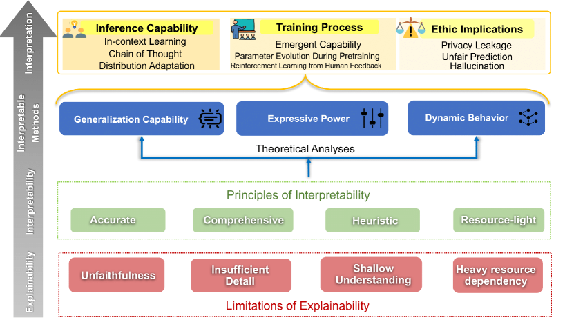
From above all, there is no universally agreed-upon definition of interpretability within the machine learning community. The concept often varies based on the application domain and the intended audience [20, 45]. This motivates us to define appropriate interpretability and develop effective interpretable methods to reveal the internal workings of FMs, as shown in Figure 1. In our perspective, the interpretability tailored for FMs refers to the ability to reveal the underlying relationships between various related factors, such as model architecture, optimization process, data and model performance, in an accurate, legible, and heuristic way. This level of interpretability can significantly enhance public confidence in model components, mitigate potential risks, and drive continuous improvement of these black-box models. To achieve this, we will develop interpretable methods tailored for FMs, grounded in rigorous learning theory. These methods will encompass analyses of generalization performance, expressivity, and dynamic behavior. Generalization performance analysis, a form of uncertainty quantification, is the process of evaluating a foundation model’s ability to accurately predict or classify new, unseen data. Expressivity analysis is the process of evaluating a model’s capacity to represent complex patterns and functions within the data. Dynamic behavior analysis involves capturing the transformations and adaptations that occur within FMs as they learn from data, makes predictions, and undergoes training iterations. These interpretable methods align with the principles of interpretability as they:
-
•
Accurate. Compared to explainable methods based on post-hoc explanation, theoretical analysis, grounded in stringent mathematical or statistical principles, has the ability to predict the expected performance of algorithms under various conditions, ensuring accuracy and faithfulness in their assessments.
-
•
Comprehensive. The insights drawn from theoretical constructs are typically more comprehensive, delving into the multidimensional influences on model performance from a holistic viewpoint. For instance, within the realm of model generalization analysis, we can discern the intricate ways in which factors like optimization algorithms and model architecture shape and impact the model’s ability to generalize effectively.
-
•
Heuristic. Theoretical analyses can provide heuristic insights by distilling complex information into practical rules, guidelines, or approximations that facilitate decision-making, problem-solving, and understanding of complex systems. These insights are derived from a deep understanding of the underlying principles but are presented in a simplified and practical form for application in real-world scenarios.
-
•
Resource-light. Theoretical analyses in machine learning are regarded as resource-light because they emphasize understanding fundamental concepts, algorithmic properties, and theoretical frameworks through mathematical abstractions. This approach stands in contrast to explainable methods that entail heavy computational demands for training additional models.
for tree= grow=east, draw, rounded corners, node options=align=center, minimum width=2cm, text centered, edge=->, thick, edge path= [draw, \forestoptionedge] (!u.east) -| +(+5pt,0) |- (.child anchor) \forestoptionedge label; , s sep+=1pt [ Interpretation for FMs, text width=2cm, minimum width=0.5cm, minimum height=0.5cm [Ethic Implications - Section 5 [Hallucination [Detection of hallucination [46, 47, 48, 49, 50, 51], fill=orange!5] [Cause of hallucination [52], fill=orange!5] ] [Unfair prediction [Generalization analysis [53, 54, 55, 56, 57], fill=orange!5] [Evaluation metric [58, 59], fill=orange!5] ] [Privacy leakage [Differential privacy and generalization [60, 61, 62, 63, 64, 65, 66, 67, 68, 69], fill=orange!5] [Memorization and generalization [70], fill=orange!5] ] ] [Training Process - Section 4 [Reinforcement Learning from Human Feedback, text width=4cm [Online RLHF [2, 71, 72, 73, 74, 75], fill=orange!5 ] [Offline RLHF [76, 77, 78], fill=orange!5 ] [Dueling Bandits [79, 80], fill=orange!5] ] [Parameter Evolution [Training Dynamics [81, 82, 83, 84, 85, 86, 87], fill=orange!5] ] [Emergent Capability [Quantify Emergence [88, 89], fill=orange!5] [Triggers of Emergence [90, 16], fill=orange!5] ] ] [Inference Capability - Section 3 [Distribution Shifts [Covariate Shifts [91, 92], fill=orange!5 ] [Query Shifts [91], fill=orange!5 ] [Task Shifts [93, 91, 94, 95, 96], fill=orange!5 ] ] [Chain-of-Thought [Expressivity Analysis of CoT [97, 98, 99, 100], fill=orange!5] [Generalization Analysis for CoT [101], fill=orange!5] ] [In-Context Learning, text width=2cm [Expressivity Analysis, text width=2cm [ Expressivity of ICL [102, 103, 104, 105, 106], fill=orange!5 ] ] [Generalization Analysis, text width=2cm, minimum width=0.1cm, minimum height=0.5cm [Algorithmic Stability [93, 107], fill=orange!5] [PAC-Bayes arguments [108], fill=orange!5] [Covering numbers [105, 109], fill=orange!5] [Gradient Flow Based [110, 111, 112], fill=orange!5] ] ] ] ]
The structure of this paper is as follows (for a visual representation of the overall framework, please see Figure 2): Section 2 reviews key interpretable methods, including analyses of generalization performance, expressivity, and dynamic behavior. Section 3 delves into the inference capabilities of FMs, exploring in-context learning, CoT reasoning, and distribution adaptation. Section 4 provides detailed interpretations of FMs training dynamics. Section 5 focuses on the ethical implications of FMs, including privacy preservation, fairness, and hallucinations. Finally, Section 6 discusses future research directions based on the insights gained from the aforementioned interpretations.
2 Interpretable Methods
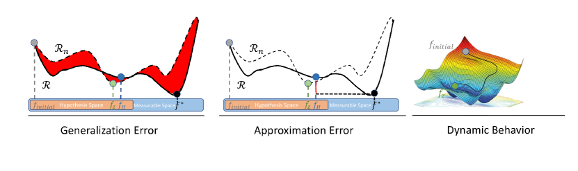
In this section, we introduce three interpretable methods grounded in rigorous machine learning theory, namely generalization analysis, expressive power analysis, and dynamic behavior analysis (as shown in Figure 3) [113, 114, 115]. These methods provide a systematic theoretical framework for analyzing the complex behaviors of FMs spanning from training to inference phases. This includes interpreting phenomena like ICL learning and CoT reasoning, as well as addressing ethical implications such as privacy leakage, unfair prediction, and hallucinations. With the heuristic insights from these interpretations, we can further refine these powerful models.
2.1 Generalization Analysis
Generalization error measures the performance of a machine learning model on unseen data. Mathematically, for a hypothesis and a dataset , the generalization error can be expressed as:
where denotes the data distribution, is the loss function, and represents the learning algorithm. Lower generalization error bound indicates a model that better generalizes from the training data to new data, thereby enhancing its predictive performance on real-world tasks.
Usually, excess risk, a directly related concept to generalization error are used to quantify the difference between the expected loss of a model on the training data and the expected loss of the best possible model on the same data. Mathematically, it can be expressed as:
If the excess risk is small, it implies that the model is not overfitting to the training data and can generalize well to unseen data. Excess risk is a direct upper bound on generalization error. This means that if you can control the excess risk, you can also control the generalization error.
Usually, generalization error depends on the complexity of the hypothesis space [116]. Following this approach, a series of works have examined the VC-dimension and Rademacher complexity to establish the upper bounds on the generalization error.
VC-dimensition.
The Vapnik-Chervonenkis dimension (VC-dimension, [117, 118, 119])
is an expressive capacity measure for assessing the hypothesis complexity. The pertinent definitions are presented below.
Definition 2.1.
For any non-negative integer , the growth function of a hypothesis space is defined as follows:
| (1) |
If , the dataset is shattered by . The VC-dimension, donated as , is the largest size of a shattered set. In other words, is the largest value of such that . If there does not exist a largest such , we define .
Elevated VC dimensions correlate with the model’s increased capability to shatter a wider range of samples, enhancing expressive capacity. Through the VC dimension, one can establish a uniform generalization bound as follows [120]. Specifically, assume the hypothesis space has VC-dimension . Then, for any , the following inequality holds
with probability over the choice of .
Rademacher complexity. Rademacher complexity captures the ability of a hypothesis space to fit random labels as a measure of expressive capacity [120, 121]. An increased Rademacher complexity signifies higher hypothesis complexity and, correspondingly, an augmented capacity for model expressiveness. The common definition are presented below.
Definition 2.2 (Empirical Rademacher complexity).
Given a real-valued function class and a dataset , the empirical Rademacher complexity is defined as follows,
where are i.i.d. Rademacher random variables with .
One can establish a worst-case generalization error bound via the Rademacher complexity. Specifically, for a loss function with an upper bound of , for any , with probability at least , the following holds for all ,
Both [122] and [123] indicate that deep learning models commonly display overparameterization in practical settings, possessing a vastly greater number of parameters than training samples. Under such overparameterized regimes, both the VC dimension and Rademacher complexity of these models tend to become excessively large. Thus, the practical utility of bounds derived from these complexity measures is relatively limited.
Algorithmic Stability. Stability concepts address these limitations and offer more refined insights into the optimization-dependent generalization behavior. Early work by [124] introduced the notion of algorithmic stability and demonstrated how it could be used to derive generalization bounds. They showed that if an algorithm is uniformly stable, meaning the output hypothesis does not change significantly with small perturbations in the training data, then it is possible to establish tight generalization bounds. Their pioneering work laid the foundation for subsequent research in understanding the stability properties of various learning algorithms and their impact on generalization performance [125, 126, 127, 128]. In particular, uniform stability and error stability are key algorithmic properties that will be utilized in the analyses presented in this section.
Definition 2.3 (Uniform stability [124]).
Let and be any two training samples that differ by a single point. A learning algorithm is -uniformly stable if
where and is the loss function.
Definition 2.4 (Error stability [124]).
A learning algorithm has error stability with respect to the loss function if the following holds:
Consequently, if algorithm is applied to two closely similar training sets, the disparity in the losses associated with the resulting hypotheses should be constrained to no more than . [127] have demonstrated that, utilizing moment bound and concentration inequality, generalization error bounds of stable learning algorithms can be derived as follows:
Theorem 2.5 (Exponential generalization bound in terms of uniform stability).
Let algorithm be -uniformly stable, and let the loss function satisfy , and . Given a training sample , for any , it holds that:
with probability at least .
PAC-Bayesian approach. PAC-Bayesian theory was initially developed by McAllester [129] to explain Bayesian learning from the perspective of learning theory. Following the exposition in [116], we assign a prior probability , or a probability density if is continuous, to each hypothesis . By applying Bayesian reasoning, the learning process establishes a posterior distribution over , denoted as In a supervised learning scenario where consists of functions mapping from to , with . Then, can be interpreted as defining a randomized prediction rule. Specifically, for a unseen example , a hypothesis is drawn according to , and the prediction is then made. The loss associated with is defined as:
Then, both the generalization loss and the empirical training loss of can be expressed as follows:
In accordance with [116], we proceed to present the following generalization bound:
Theorem 2.6.
Let be a prior distribution over hypothesis space , and be any distribution over an input-output pair space . For any and over (including those that depend on the training data ), we have:
with a probability of at least , where
is the Kullback-Leibler (KL) divergence between the distributions and
This theorem establishes a bound on the generalization error for the posterior , expressed in terms of the KL divergence between and the prior . These generalization bounds offer a promising way for interpreting the behavior of FMs associated with various optimization strategies, such as pretraining, fine-tuning and RLHF.
2.2 Expressive Power Analysis
Expressive Power traditionally refers to the ability of a neural network to represent a wide and diverse range of functions. However, with the advent of FMs, the concept of expressive power has been further expanded. For instance, the use of prompts such as chain of thought can also influence a model’s expressive capabilities. This concept is essential for evaluating the potential of FMs to capture complex structures and relationships within data.
Understanding the expressive power of FMs is particularly important for interpreting both their capabilities and limitations. As FMs are increasingly utilized in various applications, analyzing their expressive power helps us determine the range of tasks they can handle. This insight is crucial for identifying scenarios where these models are likely to excel or encounter difficulties, thereby guiding the development of more robust and versatile architectures. Moreover, a thorough examination of expressive power ensures that a model’s performance aligns with expectations, not only in traditional applications but also in novel and unforeseen scenarios.
Mathematically, expressive power can be defined in terms of a model’s ability to approximate functions within a certain class. Let denote the class of functions that a neural network can represent, parameterized by its architecture (e.g., depth, width, and activation functions). Consider a target function within a broader function space , such as the space of continuous functions over a compact domain . The hypothesis space is said to have sufficient expressive power with respect to if and , there exists a function such that:
This condition signifies that the model can approximate any function from the space with arbitrary precision, given sufficient capacity. Therefore, expressive power serves as a critical metric for understanding the theoretical capabilities of neural networks, particularly in terms of their potential to adapt, and perform complex tasks across various domains.
The commonly-used theoretical tools for analyzing the expressive power of models are as follows:
-
•
Universal Approximation Theorem: The Universal Approximation Theorem states that, with a single hidden layer and finite number of neurons, a feedforward neural network can approximate any continuous function on a compact input space to arbitrary accuracy, given a sufficiently large number of neurons. Specifically, for a neural network with a single hidden layer containing neurons, the output can be represented as
where is the weights connecting input to the -th neuron in the hidden layer, is bias term of the -th neuron in the hidden layer, and represents a nonlinear activation function. Thus, given a continuous function and a compact set , for any and , there exists a neural network with a single hidden layer and a nonlinear activation function such that
for all , where is the output of the neural network.
-
•
Expressivity in Higher Complexity Classes: Expressivity in Higher Complexity Classes examines the ability of neural networks, particularly transformers using Chain-of-Thought prompting, to solve problems within higher computational complexity classes, such as (log-space parallel computation) and (constant-depth Boolean circuits). CoT enhances a network’s ability to decompose and solve complex tasks, thereby increasing its expressiveness:
These theoretical tools play a critical role in deepening our understanding and evaluation of the expressive power of neural networks and transformer-based models.
2.3 Dynamic Behavior Analysis
Training dynamic behavior analysis is the study of how machine learning algorithms evolve over time during the training process, with a focus on understanding how parameter updates influence the convergence behavior, speed, and final quality of the solution. This analysis is crucial for optimizing the performance and reliability of machine learning models, particularly in complex scenarios involving large-scale data and deep architectures.
Following the work [114], dynamic behavior analysis can be systematically divided into three key steps. First, it ensures that the algorithm begins running effectively and converges to a reasonable solution, such as a stationary point, by examining conditions that prevent issues like oscillation or divergence. Next, it focuses on the speed of convergence, aiming to accelerate the process and reduce the computational resources and time required for training. Techniques like adaptive learning rates or momentum may be used to enhance efficiency. Finally, the analysis ensures that the algorithm converges to a solution with a low objective value, ideally achieving a global minimum rather than settling for a local one. This step is crucial for securing a high-quality final solution that generalizes well to unseen data. Additionally, several fundamental tools used for the theoretical analysis of training dynamics are as follows:
-
•
Neural Tangent Kernel (NTK): The NTK is a theoretical framework that models the training dynamics of deep neural networks in the infinite-width limit. NTK approximates the training process by treating the network as a linear model with a fixed kernel, defined by
where is the network output, represents the network parameters, and and are input samples. The NTK captures the evolution of the network’s output during gradient descent and is instrumental in understanding the expressive capabilities of neural networks.
-
•
(Stochastic) Differential Equation: Gradient flow represents the continuous-time analog of gradient descent, described by the differential equation:
This mathematical approach allows for a smooth analysis of the training dynamics, modeling how parameters evolve continuously over time and providing deeper insights into the convergence behavior of the algorithm.
3 Interpreting Inference Capabilities of Foundation Models
In this section, we aim to leverage the interpretable methods discussed in Section 2 to interpret the fundamental causes driving impressive inference capability of FMs, including ICL, CoT, and adaptability to distribution shifts.
3.1 In-Context Learning
As models and their training datasets have grown in complexity, FMs have demonstrated remarkable capabilities, notably in ICL [130]. ICL allows models to learn from a few demonstrations provided in the input context, enabling them to handle complex tasks without parameter updates, as seen in mathematical reasoning problems [5]. Unlike supervised learning, ICL leverages pretrained FMs for prediction without requiring a dedicated training phase. Formally, ICL is defined as follows.
Definition 3.1.
In a formal framework, the process takes a query input and a set of candidate answers , where may represent class labels or a collection of free-text expressions. A pre-trained model generates the predicted answer by conditioning on a demonstration set alongside the query input . The demonstration set encompasses demonstration examples , where each represents an in-context example aligned with the task at hand. The answer is modeled by a pre-trained function , defined as:
where is the parameter of the pre-trained model. The function outputs the current answer given the demonstration and the query input.
Based upon the above definition, the generalization of FMs under ICL can be measured by the upper bound on population risk. In the most common practical setting, where predictions are made at every position, the population risk is defined as follows:
Moreover, for the scenario where predictions are made after observing a fixed length of demonstration examples, the population risk is defined as follows:
where is the loss function and . Despite the impressive performance of FMs with ICL prompts, significant confusions persist from a layman, user or even researcher perspective. These challenges primarily revolve around the sensitivity of ICL to minor prompt variations and the difficulty of constructing effective in-context examples to achieve desired outputs.
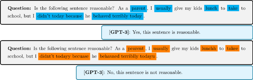
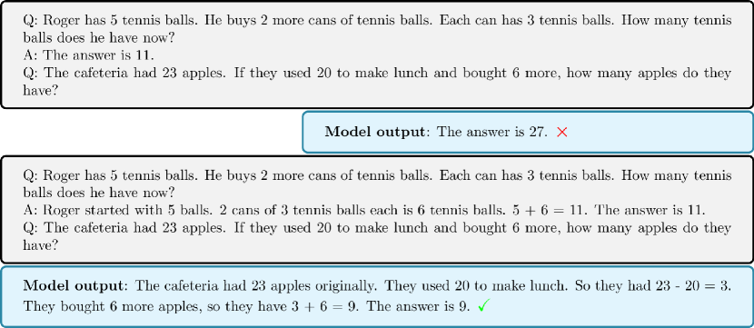
Sensitivity to Prompt Variations. A critical challenge is understanding why small differences in the input can produce significantly different outputs. For instance, a prompt containing typographical errors or slight changes in structure might not only confuse the model but can also result in drastically inaccurate responses. This phenomenon reflects the underlying mechanics of FMs, which heavily depend on precise token sequences for accurate interpretation. As shown in Fig. 4, a simple prompt with minor errors, such as incorrect spelling, can cause the model to misinterpret the entire context, thereby affecting the final output.
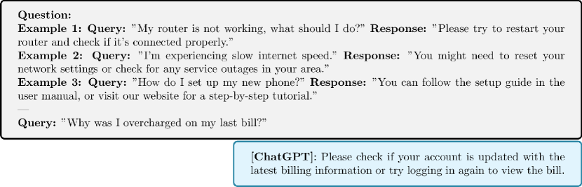
Constructing Effective In-Context Examples. Another challenge lies in constructing effective in-context examples that align with the user’s expectations. Users often struggle with determining the appropriate length and specificity of examples to include in the prompt. The relevance and level of detail in these examples are critical factors that directly impact the quality and accuracy of the model’s responses. For instance, as illustrated in Fig. 5, when a FM is used to automatically generate customer service responses, providing examples that primarily focus on technical support may lead to errors when the query is about billing issues. In such cases, the model might incorrectly categorize the billing query as a technical problem, resulting in an irrelevant or inaccurate response. Therefore, users must carefully craft examples that provide enough detail to guide the model accurately and ensure that these examples are directly aligned with the nature of the query.
To address these concerns, the analyses of generalization and expressivity can be utilized to offer insights into optimizing the responses of FMs by adjusting the structure and content of input examples within ICL.
3.1.1 Interpreting Through Generalization Analysis
Recently, various theoretical perspectives on the generalization of FMs under ICL have been explored [111, 109, 93, 108, 92, 94, 110, 105, 132]. Since FMs rely on the context provided during inference to perform tasks, these theoretical frameworks offer valuable insights into how models generalize to novel tasks without requiring additional training. They highlight the pivotal importance of model architecture, pretraining methodologies, and input context structure in driving this generalization. In this section, we review and interpret relevant studies on FMs from the perspective of generalization error, focusing on several key approaches. One line of work explores the dynamics of gradient flow over the loss function. Another major strand of research applies statistical learning principles, including algorithmic stability, covering numbers, and PAC-Bayes theories. These methods offer different avenues for understanding the fundamental mechanisms behind in-context learning and model generalization.
In this line of research examining gradient flow behavior over the loss function, the primary focus remains on linear problem settings. To rigorously analyze gradient flow dynamics, studies like [110] often simplify the transformer architecture to a single-layer attention mechanism with linear activation functions. Specifically, [110] assumes that the parameters of a linear task are drawn from a Gaussian prior, , and the prompt is an independent copy of the testing sample , where , , and . Furthermore, they consider a pretraining dataset where each of the independent regression tasks is associated with in-context prompt examples. The generalization is defined as , establishing a sample complexity bound for the pretraining of a linear parameterized single-layer attention model within the framework of linear regression under a Gaussian prior. The theorem is stated as follows:
Theorem 3.2.
(Task complexity for pertaining [110]). Let represent the quantity of in-context examples utilized to generate the dataset. Let denote the parameters output by SGD on the pretraining dataset with a geometrically decaying step size. Assume that the initialization commutes with and , where is an absolute constant and is defined as . Then we have
| (2) |
where the effective number of tasks and effective dimension are given by
respectively. Here, and represent the eigenvalues of and , which satisfy the following conditions:
The theorem above demonstrates that SGD-based pretraining can efficiently recover the optimal parameter given a sufficiently large . Referring to the first term in Equation 2, the initial component represents the error associated with applying gradient descent directly to the population ICL risk , which decays exponentially. However, given the finite number of pretraining tasks, directly minimizing the population ICL risk is not possible, and the second term in Equation 2 accounts for the uncertainty (variance) arising from pretraining on a finite number of distinct tasks. As the effective dimension of the model shrinks compared to the number of tasks, the variance also decreases. Importantly, the initial step size balances the two terms: increasing the initial step size reduces the first term while amplifying the second, whereas decreasing it has the opposite effect. Their theoretical analysis indicates that the attention model can be efficiently pre-trained using a number of linear regression tasks independent of the dimension. Furthermore, they show that the pre-trained attention model performs as a Bayes-optimal predictor when the context length during inference closely matches that used in pretraining.
Additionally, [111] revisits the training of transformers for linear regression, focusing on a bi-objective task that involves predicting both the mean and variance of the conditional distribution. They investigate scenarios where transformers operate under the constraint of a finite context window capacity and explore the implications of making predictions at every position. This leads to the derivation of a generalization bound expressed as
where denotes the length of the demonstration examples. Their analysis utilizes the structure of the context window to formulate a Markov chain over the prompt sequence and derive an upper bound for its mixing time.
Another significant line of research employs statistical learning theory techniques, including covering numbers, PAC-Bayes arguments, and algorithm stability [105, 109, 108, 93]. Specifically, [105] and [109] utilize chaining arguments with covering numbers to derive generalization bounds. In [105], the authors employ standard uniform concentration analysis via covering numbers to establish an excess risk guarantee. Specifically, they consider embedding dimensions , the number of layers , the number of attention heads , feedforward width , and the norm of parameters . Furthermore, they explore the use of prompts where each has in-context examples for pretraining, leading to the derivation of the following excess risk bound:
Theorem 3.3.
(Excess risk of Pretraining [105]). With probability at least over the pretraining instances, the ERM solution to satisfies
Furthermore, regarding sparse linear models such as LASSO, under certain conditions, it can be demonstrated that with probability at least over the training instances, the solution of the ERM problem, with input , possessing layers, attention heads, , and represents the standard deviation of the labels in the Gaussian prior of the in-context data distribution, ultimately achieves a smaller excess ICL risk, i.e.,
It is important to highlight that the theoretical result in Theorem 3.3 of research [105] deviates from the standard transformer architecture by substituting the softmax activation in the attention layers with a normalized ReLU function. This differs from the findings in Theorem 3.2 of research [133], which adheres to the standard architecture. Furthermore, [109] also employs the standard transformer architecture with softmax activation, focusing on a more specific context involving sequential decision-making problems. It utilizes covering arguments to derive a generalization upper bound of for the average regret.
Additionally, under PAC-Bayes framework, [108] investigate the pretraining error and draw a link between the pretraining error and ICL regret. Their findings show that the total variation distance between the trained model and a reference model is bounded as follows:
Theorem 3.4.
(Total Variation Distance [108]) Let represent the probability distribution induced by the transformer with parameter . Additionally, the model is pretrained by the algorithm:
Furthermore, they consider the realizable setting, where ground truth probability distribution and are consistent for some . Then, with probability at least , the following inequality holds:
| (3) |
where denotes the total variation (TV) distance.
This result is achieved through a concentration argument applied to Markov chains, providing a quantifiable measure of model deviation during pretraining. They also interpret a variant of the attention mechanism as embedding Bayesian Model Averaging (BMA) within its architecture, enabling the transformer to perform ICL through prompting.
Further, we expand on the use of stability analysis to interpret the generalization of FMs during ICL prompting. Recently, there has been growing interest in formalizing ICL as an algorithm learning problem, with the transformer model implicitly forming a hypothesis function during inference. This perspective has inspired the development of generalization bounds for ICL by associating the excess risk with the stability of the algorithm executed by the transformer [93, 111, 107].
Several studies have investigated how the architecture of transformers, particularly the attention mechanism, adheres to stability conditions [111, 107]. These works characterize when and how transformers can be provably stable, offering insights into their generalization. For instance, it has been shown that under certain conditions, the attention mechanism in transformers can ensure that the model’s output remains stable even when small changes are introduced in the training data [93]. This stability, in turn, translates into better generalization performance, making transformers a powerful tool in various applications requiring robust predictions from complex and high-dimensional data.
Next, we demonstrate that, during ICL prompting, a multilayer transformer satisfies the stability condition under mild assumptions, as indicated by the findings in [93]. This property is critical for maintaining robust generalization performance, as it implies that the model’s predictions remain stable and reliable despite minor perturbations in the training dataset.
Theorem 3.5 (Stability of Multilayer Transformer ([93])).
The formal representation of the -th query and in-context examples in the -th prompt is , where . Let and be two prompts that differ only at the inputs and where . Assume that inputs and labels are contained inside the unit Euclidean ball in . These prompts are shaped into matrices and , respectively. Consider the following definition of as a -layer transformer: Starting with , the -th layer applies MLPs and self-attention, with the softmax function being applied to each row:
Assume the transformer is normalized such that and , and the MLPs adhere to with . Let output the last token of the final layer corresponding to the query . Then,
Thus, assuming the loss function is -Lipschitz, the algorithm induced by exhibits error stability with .
Additionally, we need to provide further remarks regarding this theorem [93]. While the reliance on depth is growing exponentially, this constraint is less significant for most transformer architectures, as they typically do not have extreme depths. For instance, from 12 to 48 layers are present in various versions of GPT-2 and BERT [134, 135]. In this theorem, the upper bound on ensures that no single token can exert significant influence over another. The crucial technical aspect of this result is demonstrating the stability of the self-attention layer, which is the core component of a transformer. This stability is essential for maintaining the integrity and performance of the model, as it ensures that the influence of any individual token is limited, thereby preserving the overall structure and coherence of the model’s output.
Assume the model is trained on tasks, each including a data sequence with examples. Each sequence is input to the model in an auto-regressive manner during training. By conceptualizing ICL as an algorithmic learning problem, [93] derive a multitask generalization rate of for i.i.d. data. To establish the appropriate reliance on sequence length (the factor), they address temporal dependencies by correlating generalization with algorithmic stability. Next, we introduce the excess risk bound, which quantifies the performance gap between the learned model and the optimal model. This measure accounts for both generalization error and optimization error, providing a comprehensive evaluation of the model’s effectiveness.
Theorem 3.6 (Excess Risk Bound in [93]).
For all tasks, let’s assume that the set of algorithmic hypotheses is -stable as defined in 2.4, and that the loss function is -Lipschitz continuous, taking values in the interval . Allow to stand for the empirical solution that was acquired. Afterwards, the following bound is satisfied by the excess multi-task learning (MTL) test risk with a probability of at least :
The term denotes the -covering number of the hypothesis set , utilized to regulate model complexity. In this context, represents the prediction disparity between the two algorithms on the most adverse data sequence, governed by the Lipschitz constant of the transformer design. The bound in 3.6 attains a rate of by encompassing the algorithm space with a resolution of . For Lipschitz architectures possessing trainable weights, it follows that . Consequently, the excess risk is constrained by up to logarithmic factors, and will diminish as and go toward infinity.
It is worth noting that [93] addresses the multi-layer multi-head self-attention model, whereas [107] derives convergence and generalization guarantees for gradient-descent training of a single-layer multi-head self-attention model through stability analysis, given a suitable realizability condition on the data.
Further contributions have explored how ICL can be framed as a process of searching for the optimal algorithm during the training phase, while research on the inference phase has demonstrated that generalization error tends to decrease as the length of the prompt increases. Although these studies provide valuable insights into interpreting the performance of FMs through the lens of ICL’s generalization abilities, they often remain limited to simplified models and tasks. There is still a need for more in-depth research, particularly in understanding the impact of various components within complete transformer architectures and extending these analyses to more complex tasks. This deeper exploration could lead to a more comprehensive understanding of how foundation models achieve their impressive generalization performance across a wider range of scenarios.
3.1.2 Interpreting Through Expressivity Analysis
The utilization of prompts plays a crucial role in enhancing the expressive capabilities of FMs, particularly through techniques such as ICL prompting.
Recent research has provided significant insights into the ICL capabilities of transformers, establishing a link between gradient descent (GD) in classification and regression tasks and the feedforward operations within transformer layers [136]. This relationship has been rigorously formalized by [102], [103], and [104], who have demonstrated through constructive proofs that an attention layer possesses sufficient expressiveness to perform a single GD step. These studies aim to interpret ICL by proposing that, during the training of transformers on auto-regressive tasks, the forward pass effectively implements in-context learning via gradient-based optimization of an implicit auto-regressive inner loss, derived from the in-context data.
Specifically, research in [103] presents a construction where learning occurs by simultaneously updating all tokens, including the test token, through a linear self-attention layer. In this framework, the token produced in response to a query (test) token is transformed from its initial state , where is the initial weight matrix, to the post-learning prediction after one gradient descent step. Let , , and be the projection, value, and key matrices, respectively. The theorem is as follows:
Theorem 3.7.
(Linking Gradient Descent and Self-Attention [103]) Given a single-head linear attention layer and a set of in-context example for , it is possible to construct key, query, and value matrices , as well as a projection matrix , such that a transformer step applied to each in-context example is equivalent to the gradient-induced update , resulting in . This dynamic is similarly applicable to the query token .
Drawing from these observations, [137] have shown that transformers are capable of approximating a wide range of computational tasks, from programmable computers to general machine learning algorithms. Additionally, [138] explored the parallels between single-layer self-attention mechanisms and GD in the realm of softmax regression, identifying conditions under which these similarities hold.
The studies [96] and [91] conducted further investigation into the implementation of ICL for linear regression, specifically through the utilization of single-layer linear attention models. They demonstrated that a global minimizer of the population ICL loss can be interpreted as a single gradient descent step with a matrix step size. [106] provided a similar result specifically for ICL in isotropic linear regression. It is noteworthy that [91] also addressed the optimization of attention models; however, their findings necessitate an infinite number of pretraining tasks. Similarly, [105] established task complexity bounds for pretraining based on uniform convergence and demonstrated that pretrained transformers are capable of performing algorithm selection. Furthermore, a simplified linear parameterization was utilized in [110], which provided more refined task complexity boundaries for the purpose of pretraining a single-layer linear attention model.
That said, there remain areas in existing research that require refinement. For example, many current studies attempt to model each gradient descent step using a single attention layer within transformer architectures. This approach raises questions regarding its suitability, particularly given that transformers are typically not extremely deep. For instance, variants of models like GPT-2 and BERT usually consist of 12 to 48 layers, which constrains the number of gradient descent steps that can be effectively modeled. This limitation suggests that further investigation is needed to refine these models and better align them with the theoretical underpinnings of gradient descent in the context of ICL.
3.1.3 Concluding Remarks
In this section, we delve into the theoretical underpinnings of FMs to address the challenges users encounter when employing ICL prompts. By understanding the inner workings of FMs, we aim to provide theoretical explanations and insights that can guide practitioners and inspire future research directions.
Theoretical Interpretations of Prompt Sensitivity: One key challenge users encounter is understanding why seemingly similar prompts can lead to vastly different outputs, as shown in Figure 4. This issue can be interpreted through the stability-based generalization bounds established by [93]. From a theoretical perspective, [93] quantified the influence of one token on another and demonstrated that the stability of ICL predictions improves with an increased number of in-context examples, an appropriate (non-extreme) depth of Transformer layers, and training on complete sequences. These factors help enhance the model’s resistance to input perturbations. Furthermore, exploring the impact of introducing noisy data during training on ICL stability could be an interesting direction for future research, offering additional ways to reinforce model stability.
Constructing Effective In-Context Examples: Another major challenge for users is how to construct appropriate in-context examples as prompts, as shown in Figure 5. Numerous theoretical studies have provided insights into this challenge. Research [93, 92] suggests that longer prompts generally lead to lower generalization errors and improved performance because they offer richer contextual information that aids the model in better understanding the task. Additionally, [110] found that model performance improves when the context length during inference closely matches that of pretraining. Furthermore, when in-context examples share similar patterns or structures with the query, the model’s performance can be significantly enhanced. Specifically, the amount of influence that various parameters have on the performance of ICL generalization was quantified by [92]. These factors include the quantity of relevant features and the fraction of context instances that include the same relevant pattern as the new query.
3.2 Chain-of-Thought Reasoning
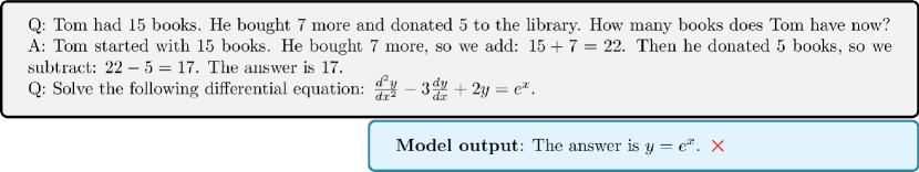
When users employ FMs for reasoning tasks involving CoT prompting, several challenges and uncertainties arise. One important question is whether CoT can effectively improve model performance in complex reasoning tasks. While CoT prompting has been shown to enable FMs to handle intricate arithmetic problems, as illustrated in Figure 7, there is still uncertainty about the generalizability of this effect. practitioners are particularly interested in understanding why CoT improves performance. This raises questions about the underlying mechanisms that allow CoT to facilitate more effective reasoning in FMs.
Another challenge involves determining the optimal prompt structure to leverage CoT for accurate results. Users are often uncertain about how many steps or how detailed the prompts need to be for the model to fully utilize CoT and produce correct inferences. This uncertainty makes it difficult for users to craft effective prompts that guide the model towards the desired outcome.
Additionally, users face challenges when they cannot provide precise reasoning samples. In such scenarios, they wonder whether CoT remains effective. This uncertainty about the robustness of CoT, particularly when ideal samples are not available, poses a significant challenge for users attempting to harness the full potential of FMs for complex reasoning tasks. As illustrated in the Figure 6, when the reasoning samples involve only simple arithmetic, but the query requires solving a complex differential equation, CoT reasoning in FMs fails.
3.2.1 Interpreting Through Generalization Analysis
The CoT method [5] enhances a model’s reasoning capabilities by guiding it through a structured, step-by-step problem-solving process. This approach is particularly effective for tasks that require multi-step reasoning, such as logical puzzles and complex question-answering scenarios. By prompting the model to generate intermediate steps, CoT facilitates more accurate conclusions through a sequence of structured thought processes.
Numerous studies [99, 97, 98] investigate the training of Transformer models to develop CoT capabilities for evaluating novel data and tasks. In this context, we articulate the supervised learning framework proposed in [101], which utilizes pairs of prompts and labels. For each prompt-output pair associated with a task , we construct a prompt that integrates the query input by incorporating reasoning examples alongside the initial steps of the reasoning query. The formulation of the prompt for the query input is expressed as follows:
where is the -th context example,and is the first steps of the reasoning query for any in . We have and for with a notation .
From this setting, it can be observed that CoT emphasizes demonstrating intermediate reasoning steps in the problem-solving process, while referring to the definition from the section 3.1, ICL focuses on learning task mappings directly by leveraging several input-output pairs provided in the context. In certain scenarios, ICL can be regarded as a simplified reasoning process without intermediate steps, whereas CoT represents an enhanced version with multi-step reasoning [101].
To interpret the theoretical underpinnings of how transformers can be trained to acquire CoT capabilities, [101] offers a comprehensive theoretical analysis focused on transformers with nonlinear attention mechanisms. Their study delves into the mechanisms by which these models can generalize CoT reasoning to previously unseen tasks, especially when the model is exposed to examples of the new task during input. Specifically, they consider a learning model that is a single-head, one-layer attention-only transformer. The training problem is framed to enhance reasoning capabilities, addressing the empirical risk minimization defined as
where represents the number of prompt-label pairs and denotes model weights. The loss function utilized is the squared loss, specifically given by where denotes the output of the transformer model. Furthermore, following the works of [99, 97, 98, 101], the CoT generalization error for a testing query , the testing data distribution , and the labels on a -step testing task is defined as
where are the model’s final outputs presented as the CoT results for the query. They further quantify the requisite number of training samples and iterations needed to instill CoT capabilities in a model, shedding light on the computational demands of achieving such generalization. Specifically, they describe the model’s convergence and testing performance during the training phase using sample complexity analysis, as detailed in the following theorem:
Theorem 3.8.
(Training Sample Complexity and Generalization Guarantees for CoT [101]) Consider training-relevant (TRR) patterns , which form an orthonormal set . The fraction of context examples whose inputs share the same TRR patterns as the query is denoted by . For any , when (i) the number of context examples in every training sample is
(ii) the number of SGD iterations satisfies
and (iii) the training tasks and samples are selected such that every TRR pattern is equally likely in each training batch with batch size , the step size and samples, then with a high probability, the returned model guarantees
| (4) |
where denotes the set of all model weights. Furthermore, as long as (iv) testing-relevant (TSR) patterns satisfy
for , and (v) the number of testing examples for every test task is
| (5) |
where represents the fraction of context examples whose inputs exhibit the same TSR patterns as the query. The term denotes the primacy of the step-wise transition matrices, while refers to the min-max trajectory transition probability. Finally, we have
| (6) |
This theorem elucidates the necessary conditions and properties that facilitate CoT generalization. It establishes that, to train a model capable of guaranteed CoT performance, the number of context examples per training sample, the total number of training samples, and the number of training iterations must all exhibit a linear dependence on . This finding supports the intuition that CoT effectiveness is enhanced when a greater number of context examples closely align with the query. Moreover, the attention mechanisms in the trained model are observed to concentrate on testing context examples that display similar input TSR patterns relative to the testing query during each reasoning step. This focus is a pivotal characteristic that underpins the efficacy of CoT generalization.
Additionally, to achieve a zero CoT error rate on test tasks utilizing the learned model, Equation 5 indicates that the requisite number of context examples associated with task in the testing prompt is inversely proportional to The minimum probability of the most probable -step reasoning trajectory over the initial TSR pattern is quantified by , whereas denotes the fraction of context examples whose inputs share the same TSR patterns as the query in this context. A larger constant indicates a higher reasoning accuracy at each step. This result formally encapsulates the notion that both the quantity of accurate context examples and their similarity to the query significantly enhance CoT accuracy.
Furthermore, [99] demonstrate, the success of CoT can be attributed to its ability to decompose the ICL task into two phases: data filtering and single-step composition. This approach significantly reduces the sample complexity and facilitates the learning of complex functions.
3.2.2 Interpreting Through Expressivity Analysis
CoT prompting further amplifies expressive capabilities by guiding the model through a structured reasoning process. Following this observation, research has shifted towards comparing the task complexity between reasoning with CoT and that without CoT [99, 97, 98, 100]. Under the ICL framework, [99] demonstrates the existence of a transformer capable of learning a multi-layer perceptron, interpreting CoT as a process of first filtering important tokens and then making predictions through ICL. They establish the required number of context examples for achieving the desired prediction with the constructed Transformer. Additionally, studies [97, 98, 100] reveal that transformers utilizing CoT are more expressive than those without CoT.
In detail, [97] consider tasks on evaluating arithmetic expressions and solving linear equations. They demonstrate that the complexity of the problems is lower bounded by (Nick’s Class 1), indicating that no log-precision autoregressive Transformer with limited depth and hidden dimension could solve the non-CoT arithmetic problem or non-CoT equation problem of size if (Threshold Circuits of Constant Depth 0). Conversely, they construct autoregressive Transformers with finite depth and hidden dimension that solve these two problems in CoT reasoning. In the context of iterative rounding, [98] expands the analysis to constant-bit precision and establishes (Alternating Circuit of Depth 0) as a more stringent upper bound on the expressiveness of constant-depth transformers with constant-bit precision. On the other hand, [100] considers the impact of the chain length in the CoT process. They prove that logarithmic intermediate steps enhance the upper bound of computational power to (log-space), increasing the intermediate steps to linear size enhances the upper bound within , and polynomial sizes have upper bound (Polynomial Time).
By breaking down complex tasks into intermediate steps, CoT allows the model to articulate its thought process clearly and logically. This structured prompting not only improves the accuracy of the model’s responses but also enables it to handle intricate, multi-step problems with greater finesse.
3.2.3 Concluding Remarks
In this section, we delve into the theoretical underpinnings of FMs to address the challenges users encounter when employing CoT prompts. We aim to provide theoretical explanations and insights that can guide practitioners and inspire future research directions about CoT.
CoT-driven Expressive Capabilities Enhancement: A body of research has demonstrated that CoT significantly enhances the expressive capabilities of FMs. For example, [97] examined the expressiveness of FMs utilizing CoT in addressing fundamental mathematical and decision-making challenges. The researchers initially presented impossibility results, demonstrating that bounded-depth transformers cannot yield accurate solutions for fundamental arithmetic tasks unless the model size increases super-polynomially with input length. Conversely, they developed an argument demonstrating that constant-sized autoregressive transformers can successfully satisfy both requirements by producing CoT derivations in a standard mathematical language format. This effectively demonstrates that CoT improves the reasoning capabilities of FMs, particularly in mathematical tasks. Additionally, other studies, such as [100] and [98], have shown that CoT-based intermediate generation extends the computational power of FMs in a fundamental way. These findings reinforce the idea that CoT prompting enhances model performance by allowing FMs to break down complex reasoning processes into manageable steps, thereby enabling more accurate outcomes.
CoT Prompt Construction: How can we construct prompts that effectively leverage CoT to achieve accurate results? [101] demonstrated that, to guarantee CoT functionality, the number of context examples per training sample, the total number of training samples, and the number of training iterations must all scale linearly with the inverse of the proportion of context examples whose inputs share the same TRR patterns as the query. This aligns with the intuitive understanding that CoT performance improves when more context examples are similar to the query. When users are unable to provide precise reasoning samples, they may question the effectiveness of CoT, as shown in Figure 6. [101] addressed this concern by demonstrating that, when reasoning examples contain noise and inaccuracies, achieving zero CoT error on certain tasks requires a number of context examples that is proportional to the inverse square of the product of several factors. These factors include the fraction of accurate context examples and the similarity between the context examples and the query. This result formalizes the intuition that more accurate and relevant context examples, even in the presence of noise, significantly enhance CoT accuracy.
3.3 Adaptation to Distribution Shift
From a user’s perspective, FMs face significant challenges when dealing with distribution shifts. A common issue arises when users are unable to provide prompts that accurately align with the query. FMs often depend on prompts that mirror the data they were trained on, so when prompts deviate from this, the model’s performance can suffer, leading to inaccurate or irrelevant outputs. Below, we outline the primary challenges users encounter.
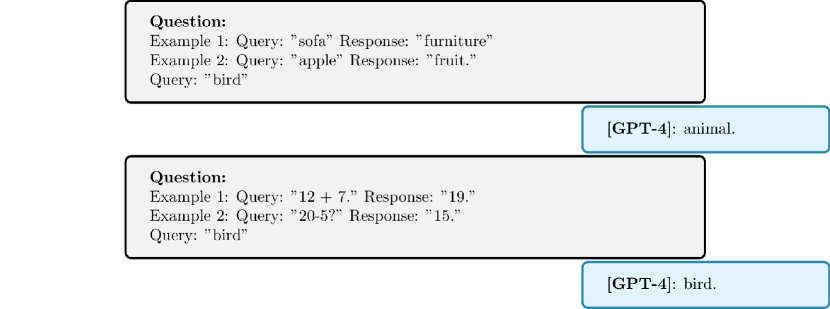
Handling Inaccurate Prompts. A frequent issue arises when users are unable to provide prompts that accurately align with the query. FMs often depend on prompts that reflect the structure and data they were trained on. When prompts deviate from these familiar patterns, the model’s performance can suffer, leading to inaccurate or irrelevant outputs. As shown in Figure 8, in an extreme case where the in-context example involves arithmetic, but the query is about birds, the foundation model struggles to provide a reasonable response when there is a complete mismatch between the in-context example and the query.
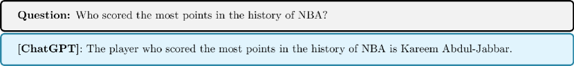
Limitations in Providing Real-Time or Updated Information. Another key challenge arises when users require the most current information, which FMs are often unable to provide. Since these models are typically trained on static datasets that are periodically updated, they often lack access to the most recent data or real-time information. For instance, as illustrated in Figure 9, questions such as "Who scored the most points in NBA history?" or "Who is the richest person in the world?" often require up-to-date answers. However, due to the lag in data updates, the model might provide outdated or incorrect information, failing to meet the user’s need for timely responses. This limitation highlights the difficulty users face when relying on foundational models for information that evolves over time.
Struggles with Uncommon Tasks. FMs also face difficulties when confronted with uncommon or novel tasks. Users may question whether the model can handle tasks it wasn’t explicitly trained for. When asked to solve rare or unique problems, the model’s performance may degrade, raising concerns about its ability to generalize to new or unfamiliar domains.
Next, we will explore how generalization analysis can be used to interpret FM’ performance under different distribution shifts, addressing the challenges and concerns users face in these scenarios.
3.3.1 Interpreting Through Generalization Analysis
Theoretical analysis of FMs under distribution shifts across various prompts can help interpret their remarkable out-of-distribution generalization capabilities. Although deep learning theory typically assumes that training and test distributions are identical, this assumption often does not hold in real-world scenarios, leading to models that may struggle to generalize effectively [139]. Due to the remarkable ability of attention-based neural networks, such as transformers, to exhibit ICL, numerous studies have theoretically investigated the behavior of trained transformers under various distribution shifts [91, 109, 93, 92, 94, 95]. These studies delve into various distribution shifts that were initially examined experimentally for transformer models by [140].
Building on the methodologies outlined in [140, 91], we focus on the design of training prompts structured as . In this framework, we assume that and . For test prompts, we assume , ,and . Next, we will explore the generalization ability of transformers under the ICL setting from three perspectives: task shifts [93, 91, 94, 95], query shifts [91], and covariate shifts [91, 92].
Task Shifts: Numerous studies have attempted to investigate the impact of task shift on generalization theoretically. [91] delve into the dynamics of ICL in transformers trained via gradient flow on linear regression problems, with a single linear self-attention layer. They demonstrate that task shifts are effectively tolerated by the trained transformer. Their primary theoretical results indicate that the trained transformer competes favorably with the best linear model, provided the prompt length during training and testing is sufficiently large. Consequently, even under task shift conditions, the trained transformer generates predictions with errors comparable to the best linear model fitting the test prompt. This behavior aligns with observations of trained transformers by [140].
Additionally, [94] propose a PAC-based framework for in-context learnability and utilize it to present the finite sample complexity results. They utilize their framework to demonstrate that, under modest assumptions, when the pretraining distribution consists of a combination of latent tasks, these tasks can be effectively acquired by ICL. This holds even when the input significantly diverges from the pretraining distribution. In their demonstration, they show that the ratio of the prompt probabilities, which is dictated by the ground-truth components, converges to zero at an exponential rate. This rate depends on the quantity of in-context examples as well as the minimum Kullback–Leibler divergence between the ground-truth component and other mixture components, indicating the distribution drift.
In contrast to the aforementioned studies focusing on task shift, [93] and [95] explore transfer learning to evaluate the performance of ICL on new tasks. Specifically, they investigate the testing performance on unseen tasks that do not appear in the training samples but belong to the same distribution as the training tasks. Specifically, [93] theoretically establish that the transfer risk decays as , where is the number of multi-task learning tasks. This is due to the fact that extra samples or sequences are usually not able to compensate for the distribution shift caused by the unseen tasks.
Query Shifts: In addressing the issue of query shift, wherein the distribution of queries and prompts in the test set is inconsistent, [91] demonstrate that broad variations in the query distribution can be effectively managed. However, markedly different outcomes are likely when the test sequence length is limited and the query input is dependent on the training dataset. To be more specific, the prediction will be zero if the query input is orthogonal to the subspace that is spanned by the ’s. This phenomenon was prominently noticed in transformer models, as recorded by [140]. This suggests that while certain architectures can generalize across diverse distributions, their performance can be severely constrained by the alignment of the query example with the training data’s subspace, emphasizing the criticality of sequence length and data dependency in model evaluation.
Covariate Shifts: To address the issue of covariate shift, where the training and testing data distributions do not match, [91] studied out-of-domain generalization within the context of linear regression problems with Gaussian inputs. They demonstrated that while gradient flow effectively identifies a global minimum in this scenario, the trained transformer remains vulnerable to even mild covariate shifts. Their theoretical findings indicate that, unlike task and query shifts, covariate shifts cannot be fully accommodated by the transformer. This limitation of the trained transformer with linear self-attention was also noted in the transformer architectures analyzed by [140]. These observations suggest that despite the similarities in predictions between the transformer and ordinary least squares in some contexts, the underlying algorithms differ fundamentally, as ordinary least squares is robust to feature scaling by a constant.
Conversely, [92] explores classification problems under a data model distinct from that of [91]. They offer a guarantee for out-of-domain generalization concerning a particular distribution type. They provide a sample complexity bound for a data model that includes both relevant patterns, which dictate the labels, and irrelevant patterns, which do not influence the labels. They demonstrate that advantageous generalization conditions encompass: (1) out-of-domain-relevant (ODR) patterns as linear combinations of in-domain-relevant (IDR) patterns, with the sum of coefficients equal to or exceeding one, and each out-of-domain-irrelevant (ODI) pattern situated within the subspace formed by in-domain-irrelevant (IDI) patterns; and (2) the testing prompt being adequately lengthy to include context inputs related to ODR patterns. Under these conditions, the transformer could effectively generalize within context, even amongst distribution shifts between the training and testing datasets.
3.3.2 Concluding Remarks
In this section, we explore theoretical frameworks that help interpret FMs and address challenges posed by distribution shifts. These challenges often occur when FMs struggle to handle prompts that deviate from the training distribution.
The prompt-query alignment: One critical challenge arises when users are unable to provide prompts that precisely align with the query, as illustrated in Figure 8, raising the question of how FMs handle query shifts—situations where the distribution of queries differs from that of prompts in the test set. Theoretical studies [91] suggest that if the test sequence length is limited and query examples are dependent on the training data, FMs can still generalize effectively. However, when the query example is orthogonal to the subspace spanned by the training data, the model’s prediction accuracy drops significantly. This highlights the importance of prompt-query alignment for optimal model performance.
The diversity of tasks: Another significant challenge lies in task shift, where users present uncommon tasks that FMs may not have been explicitly trained on. This scenario corresponds to the theoretical task shift problem. Research [93, 91] shows that if sufficiently long prompts are provided during both training and testing, FMs can generalize well even under task shift conditions. Enhancing the diversity of tasks during the pretraining phase further strengthens the model’s ability to handle task shifts. This is because greater task diversity during training exposes the model to a broader range of problem types, thereby enhancing its adaptability to new tasks.
While FMs show strong generalization under specific conditions, FMs often struggle to provide real-time or updated information due to outdated training data, as illustrated in Figure 9. Addressing distribution shifts will require developing strategies for detecting shifts and updating models efficiently. For example, policy compliance issues, such as handling evolving terms that may become offensive over time, can benefit from such advancements.
4 Interpreting Training Process in Foundation Models
In this section, we aim to leverage the interpretable methods discussed in Section 2 to interpret the training dynamics of FMs, including emergent capabilities, parameter evolution during pretraining and reinforcement learning from human feedback.
4.1 Emergent Capabilities
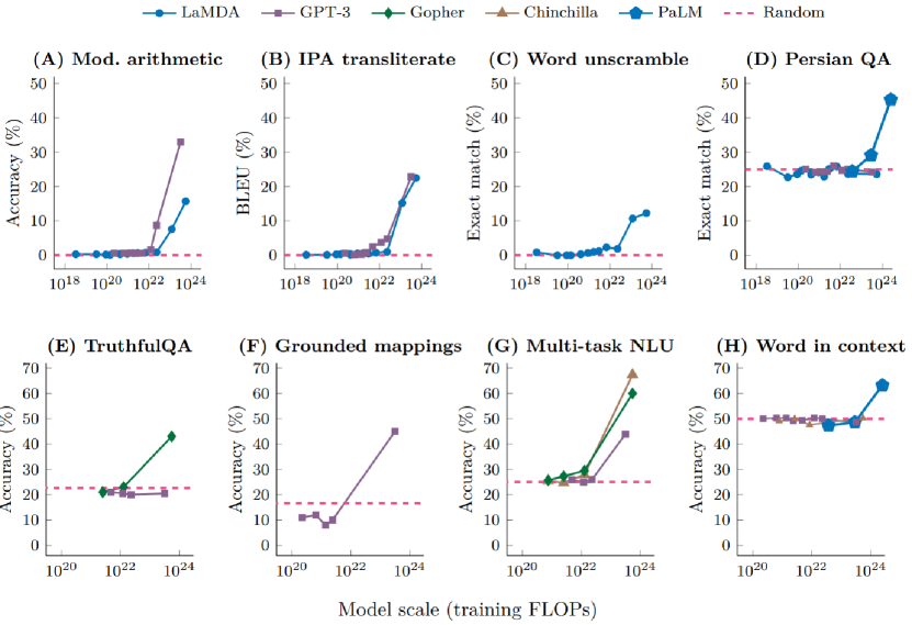
Emergent capability usually refers to the capabilities of FMs that appear suddenly and unpredictably as models scale up (see Figure 10 given by [15] for further details). Despite these advancements, significant challenges persist from the user’s perspective.
A primary concern is how to accurately measure these emergent capabilities. Users, particularly researchers and practitioners, seek clear definitions and reliable metrics to assess these abilities. Current methods often lack precision and consistency, leaving users uncertain about how to effectively evaluate emergent behaviors across different models.
Another crucial challenge involves identifying the specific conditions that trigger emergent abilities. Understanding these triggers is essential for practitioners who design and deploy FMs. They need insights into the factors that activate these capabilities, such as model size, architecture, or training data characteristics. This understanding would empower users to better harness these emergent abilities, enabling more effective model design, fine-tuning, and application in real-world tasks.
4.1.1 Interpretation for Emergent Capabilities
Emergence is among the most enigmatic and elusive characteristics of FMs [15, 16, 89], generally defined as the manifestation of “high-level intelligence” that becomes apparent only when the model reaches a sufficient scale. Originally, the emergence capabilities of FMs were described as instances where “An ability is emergent if it is not present in smaller models but is present in larger models.” by [15]. Moreover, [90] posit that the ultimate manifestations of emergent properties are ICL and zero-shot learning, where the model can comprehend task instructions provided within its input and solve the task accordingly. Early research indicates that such capabilities are abrupt and unpredictable, defying extrapolation from smaller-scale models.
However, more recent studies have demonstrated theoretically that emergence can also be observed as a smooth and continuous phenomenon. For example, [90] integrated text pieces with language skills into a bipartite random graph, applying Scaling Laws to model emergent properties across varying model sizes. They introduced a statistical framework that relates the cross-entropy loss of FMs to their competence in fundamental language tasks. Their mathematical analysis further shows that Scaling Laws imply a strong inductive bias, enabling the pre-trained model to learn very efficiently—a concept they informally refer to as “slingshot generalization.”
In addition, other work has focused on proposing a quantifiable definition of emergence in FMs. Specifically, motivated by theories in emergentism [141], [88] modeled FMs as a Markov process and defined the strength of emergence between internal transformer layers from an information-theoretic perspective. Concisely, they described emergence as a process where the entropy reduction of the entire sequence exceeds the entropy reduction of individual tokens.
Specifically, they identify the transformer block as the fundamental unit for observing the emergence phenomenon. To facilitate this analysis, they employ to index the transformer blocks within a FM, where denotes the total number of blocks. Without loss of generality, they hypothesize that the process of token representations traversing through the transformer blocks can be modeled as a Markov process. In this framework, for any transformer block , given an input sequence of token length and a hidden state dimension ,the input representation is defined as , while the output representation is denoted as , where and . The Markovian stochastic process is characterized by the transition probability which is succinctly represented as .
Furthermore, token variables in each sequence can be broadly divided into two categories: micro variables and macro variables. Micro variables correspond to individual tokens that are influenced solely by their own previous states. For instance, satisfies , meaning it is only dependent on , thus capturing local, token-specific information. In contrast, macro variables provide a more global perspective by aggregating information from all tokens in the sequence. These variables, such as , satisfy , and are influenced by every token in the sequence, reflecting the overall structure or meaning of the input. This distinction parallels the Next Token Prediction (NTP) mechanism, where the model transitions from fine-grained, token-level understanding (micro) to more holistic, sequence-level understanding (macro).
Definition 4.1.
(Emergence in FMs [88]). For any transformer block in an FM, let represent the macro variable, which captures the aggregated information across all tokens in the sequence. This macro variable follows the transition probability . Meanwhile, represents the micro variable, which corresponds to the individual token-level information and satisfies . The strength of emergence in block can be described as:
where represents the mutual information.
In this formulation, the strength of emergence is quantified by comparing the mutual information at two levels: the entropy reduction at the macro level, which represents the model’s semantic understanding, and the average entropy reduction at the micro level, which reflects token-level predictions. A larger difference between these two measures indicates a stronger emergent capability, suggesting that the model’s comprehension at the sequence level surpasses the sum of its individual token-level predictions, leading to qualitatively new behavior.
4.1.2 Concluding Remarks
In this section, we provide a theoretical interpretation of the challenges users face regarding emergent abilities in FMs. Additionally, we discuss the limitations of existing theories and suggest potential directions for future research.
Quantifying Emergent Capabilities in FMs. First, regarding the question of how to accurately measure emergent capabilities, users are particularly interested in defining and quantifying these abilities. Recent work [88] has proposed a quantifiable definition of emergence, describing it as a process where the entropy reduction of the entire sequence exceeds the entropy reduction of individual tokens. This offers a metric for evaluating emergent behaviors, although it remains limited in its generalizability across different tasks and models.
Understanding the Triggers of Emergent Capabilities in FMs. When it comes to identifying the conditions that trigger emergent abilities, research suggests that these capabilities can be explained by scaling laws. As the scale of the model increases, the model exhibits stronger inductive biases, enabling it to learn and handle complex tasks more efficiently. Theoretical insights indicate that the emergence of these abilities is not solely dependent on model size but is also closely related to task diversity and the complexity of the training data. Models are more likely to exhibit emergent abilities when faced with richer and more diverse tasks, highlighting the importance of varied and comprehensive training regimes.
However, the current understanding of emergent abilities is still in its infancy, particularly in terms of rigorous theoretical analysis of scaling laws. This reveals a gap in our knowledge of the relationship between model size and emergent capabilities, which warrants further exploration. Despite limited existing research, we posit that a promising avenue for addressing this challenge lies in mechanistic explanations grounded in mathematical analysis or control theory, such as the exploration of phase transitions in complex systems, and lévy process driven Stochastic Differential Equation (SDEs).
4.2 Parameter Evolution During Pretraining
During the pretraining phase of FMs, practitioners often seek to optimize training strategies to accelerate model convergence. A key challenge lies in identifying which training methods or configurations can effectively speed up the learning process. This includes exploring techniques such as learning rate schedules that could enhance training efficiency. Another challenge involves comprehending the parameter dynamics among various components of the transformer architecture. Questions emerge regarding the optimization dynamics within these components—how their parameters are updated and how each structure influences the overall performance of the model. Gaining insights into these internal dynamics would understand how different modules collaborate to optimize the model’s learning process, thus aiding in better development of model architecture and optimization strategies.
4.2.1 Interpretation for Pretraining Dynamics
Transformer architectures have excelled across various research domains, becoming the backbone of many FMs. A critical aspect of interpreting these models lies in understanding their training dynamics. Recent research has focused on how representations emerge from gradient-based optimization, particularly emphasizing the dynamics of individual attention layers—the core components of transformers.
The study of these dynamics was significantly advanced by research from [84], who revealed that a single attention layer trained via gradient descent can learn to encode topic structures. This discovery laid the groundwork for understanding how attention layers, through gradient-based optimization, can capture semantic information.
Expanding on the theoretical underpinnings of these mechanisms, [85, 86] established a compelling equivalence between the optimization dynamics of a singular attention layer and a particular Support Vector Machine (SVM) issue. This relationship offered a novel perspective on attention layers, indicating that they may utilize analogous optimization concepts to those present in conventional machine learning algorithms, so bridging the gap between classical techniques and modern deep learning frameworks.
Further investigation into this intersection reveals that the global optimum of a singular linear attention layer, when trained on in-context linear regression tasks, effectively executes a step of preconditioned gradient descent, as demonstrated by [96]. This finding was crucial in highlighting how linear attention layers, through their optimization dynamics, refine representations in a manner akin to classical optimization techniques, particularly in contexts where the data structure is well understood. Complementary studies by [106] and [91] focused on the specific case of in-context linear regression, providing detailed insights into how linear attention layers adjust during training to efficiently perform regression tasks. Furthermore, [112] demonstrate that gradient descent applied to a simplified two-layer transformer effectively learns to address in-context learning tasks by encoding the latent causal graph into the first attention layer.
[95] extended this exploration by demonstrating that gradient descent on a single softmax attention layer can solve linear regression problems in-context, particularly with orthogonal input data. This study underscored the flexibility of softmax attention mechanisms in adapting to different data structures through gradient-based learning, showing that attention layers are not just powerful in abstract, but also highly adaptable to specific data configurations.
The understanding of attention layers was further deepened by [87], who analyzed the gradient descent dynamics of the position block in a single-layer vision transformer. Their findings showed that this block converges to a solution that encodes spatial structure, providing important insights into how vision transformers capture and process spatial relationships within visual data. This study emphasized that even within the broader architecture of a transformer, individual components follow distinct optimization paths that contribute to the model’s overall ability to understand and represent complex data.
Moreover, [82] made significant contributions to understanding the optimization dynamics in transformer models by analyzing the behavior of a single attention layer. Specifically, they demonstrated that self-attention gradually shifts focus toward key tokens that are crucial for predicting the next token, while reducing attention to common key tokens that appear across multiple contexts. Among these distinct tokens, they identified a phase transition that can be controlled by the learning rates of the decoder and self-attention layers, leading to an almost fixed combination of tokens in the attention mechanism.
Before we delve into the specifics of the phase transition theorem, it is important to define the core variables and their roles. Let be the embedding matrix, where is the number of tokens, and is the embedding dimension. The self-attention mechanism utilizes three key projection matrices: , and , representing the query, key, and value transformations, respectively.
We define two crucial matrices derived from these projections. First, , which encodes the interactions between token pairs based on the value projections. Second, , represents the scaled dot product between queries and keys, capturing the similarity between tokens in the embedding space. The normalization factor ensures that the dot products remain in a stable range during training, preventing gradient explosion or vanishing. Then we present the theorem:
Theorem 4.2.
(Phase Transition in Training [82]). Let and denote the learning rates for the matrices and , corresponding to the decoder and self-attention layers, respectively. We also define , which evolves as , where is the entry in the -th row and -th column of representing the interaction between the query token and a contextual token . Here, is a time dependent scaling function. Additionally, define , which captures the accumulated attention dynamics over time. If the dynamics of the single common token satisfies and , then we have:
| (7) |
Here, the phase transition occurs when the training time crosses a critical threshold . The parameters and represent the learning rates of the decoder and self-attention layers, respectively. The parameter serves as a stabilizing term, while represents the number of classes or distinct tokens that the model is predicting.
-
•
For : The function grows logarithmically with time, suggesting that at the early stages of training, the model gradually refines the attention weights.
-
•
For : A phase transition occurs, leading to a significant shift in the attention patterns, where the self-attention mechanism focuses more on specific tokens, resulting in sparser attention maps.
The term quantifies the extent to which the attention mechanism evolves, and it grows as the learning rates and increase. This means that larger learning rates will accelerate the phase transition, leading to faster convergence of the attention patterns.
Furthermore, this theorem provides several insights that help interpret the training process:
-
•
Effect of Larger Learning Rate : Increasing the learning rate for the decoder layer results in a shorter phase transition time . This means that the model reaches the phase transition earlier, where the attention maps become sparser and more focused.
-
•
Scaling Up Both and : When both learning rates are scaled up, the value of becomes larger as , indicating that the attention maps become sparser over time, leading to more efficient information flow between tokens.
-
•
Small Learning Rate : If the learning rate is small while is fixed, the value of becomes larger for , which means that the attention maps will become sparser, focusing on a smaller subset of the tokens.
Thus, this theorem illustrates how different learning rates impact the phase transition during training, influencing the sparsity of attention maps and the speed at which the model converges to its final attention patterns.
In a related study, [81] demonstrated that when self-attention and MLPs are trained jointly, the resulting optimization dynamics correspond to those of a modified MLP module. This finding suggests that the interaction between different components within a transformer is critical, with each part influencing the optimization and learning behavior of the other, thus contributing to the overall model’s performance.
Finally, [83] revealed that transformers with diagonal attention matrices exhibit incremental learning behavior, suggesting that the structure of the attention matrix itself can significantly influence the learning trajectory. This finding ties back to earlier discussions on how specific configurations within the Transformer architecture can lead to distinct dynamic behaviors during training, affecting both the speed and quality of convergence.
4.2.2 Concluding Remarks
In this section, we offer theoretical insights to address the challenges previously raised by users, particularly practitioners working with FMs. Furthermore, we examine the limitations of existing theories and propose potential directions for future advancements.
Configurations That Enhance Model Learning Efficiency. Regarding the question of which training methods or configurations can accelerate model learning, recent research [83] highlights the significant impact of self-attention matrix configuration on learning trajectories. Additionally, [82] provides theoretical evidence showing that modifying the learning rates of the decoder and self-attention mechanisms can also enhance convergence rates, as outlined in Theorem 4.2. These findings suggest that strategic tuning of model components during pretraining can optimize learning efficiency.
Parameter Dynamics and Roles of Transformer Components. Another challenge concerns the parameter dynamics within different transformer components and the specific roles of these structures. Theoretical studies [82] indicate that during training, the self-attention mechanism gradually refines its focus on key tokens that are crucial for predicting the next token, while reducing attention on common tokens. This adjustment in attention improves the model’s reasoning capabilities over time. Moreover, research [81] reveals that when the self-attention mechanism and the MLP are trained together, the final optimization dynamics resemble a modified MLP module. This suggests that the interactions between different components within the transformer are critical to the model’s optimization and learning behavior. Consequently, these structures collectively influence the overall performance of the model, dynamically adjusting throughout the training process.
However, much of this research has been limited to shallow transformer architectures. To gain a more comprehensive understanding of FMs, it is crucial to extend dynamic behavior analysis to deeper transformer architectures. Exploring how these dynamics evolve in more complex, multi-layered models could provide valuable insights into the scalability of FMs and how deeper architectures enhance their expressive power. Additionally, a deeper investigation into the parameter flow and interactions between various modules within complete transformer architectures is essential for advancing our understanding of how these models optimize and function as a cohesive system.
4.3 Reinforcement Learning from Human Feedback
Although RLHF has been effective in generating models with remarkable conversational and coding capabilities, it introduces a level of complexity that surpasses that of supervised learning. The RLHF process necessitates training several language models and continuously sampling from the language model policy throughout the training loop, which results in considerable computational overhead. As a result, users are keen to explore whether more efficient methods for reward modeling can be developed to enhance model performance while reducing these computational burdens.
Moreover, RLHF practitioners face additional challenges, such as managing large state spaces with limited human feedback. This scarcity of feedback complicates the training process, making it difficult for models to learn optimal behaviors across diverse scenarios. Another challenge arises from the bounded rationality of human decisions, where human feedback may not always represent the optimal outcome, introducing noise into the training process. Lastly, practitioners must contend with off-policy distribution shift, which occurs when the data distribution used for training diverges from the actual distribution encountered during inference, potentially undermining the model’s performance.
4.3.1 Interpreting Through Dynamic Analysis
RLHF has garnered significant attention in recent years, particularly following its remarkable success in applications like ChatGPT [142]. Typically, the RLHF process is initiated after supervised finetuning (SFT). The standard procedure for aligning models with human preferences involves two main steps: reward modeling and reward maximization [143, 144, 145]. Alternatively, Direct Preference Optimization (DPO) [146, 147] offers a different approach by treating generative models directly as reward models and training them on preference data.
The theoretical basis of RLHF originates from studies on dueling bandits [79, 80], a simplified context under the RLHF paradigm. Recently, significant attention has been directed towards the more complex challenge of RLHF, also known as preference-based RLHF. Specifically, the research [2, 73, 74] investigate tabular online RLHF, characterized by a finite and constrained state space. Despite the tabular framework, [71] introduces groundbreaking findings for online RLHF utilizing general function approximation, tackling real-world issues characterized by extensive state spaces. [72] presents a reduction-based framework that modifies sample-efficient algorithms from conventional reward-based reinforcement learning to optimize algorithms for online RLHF. Additional progress in algorithm design is suggested by [75], who create reward-free learning algorithms and posterior sampling-based algorithms specifically designed for online RLHF.
In the realm of offline RLHF, [76] introduces a pessimistic algorithm that is provably efficient. Specifically, they demonstrate that when training a policy based on the learned reward model, the Maximum Likelihood Estimation (MLE) approach fails, whereas a pessimistic MLE yields policies with enhanced performance under specific coverage conditions. Their theorem is as follows:
Theorem 4.3.
Let represent the set of states (prompts) and the set of actions (responses). For each state-action pair , the reward is assumed to be parameterized by . Given certain coverage conditions, a pessimistic MLE can be constructed, resulting in an effective greedy policy ; specifically, with probability at least ,
where denotes the optimum policy associated with the true reward .
Additionally, [77] and [78] extend these explorations to the broader context of general function approximation settings within offline RLHF. Contrastingly, [147] expands related research into hybrid RLHF, considering the reverse-KL regularized contextual bandit for RLHF and proposing efficient algorithms with finite-sample theoretical guarantees in the hybrid setting.
Moreover, [148] provides substantial contributions by addressing query complexity in the process. Their algorithm attains a regret bound that optimally integrates two aspects, scaling as , where denotes the number of interactions, represents the eluder dimension of the function class, indicates the minimum preference of the optimal action over any suboptimal action across all contexts, and signifies the size of the action set. Further advancements are presented by [149], whose proposed algorithm eliminates the dependency on the action space , achieving a regret bound of .
4.3.2 Concluding Remarks
In this chapter, we primarily utilize theoretical results to interpret the underlying mechanisms of RLHF, thereby addressing the challenges. Additionally, we explore potential directions for future theoretical advancements.
Efficient Reward Modeling in RLHF. In exploring whether the reward modeling process in RLHF can be optimized to reduce computational costs and make the training pipeline more efficient, recent studies have introduced promising approaches. For instance, [146] proposed a new parameterization of the reward model in RLHF, known as DPO, which allows the extraction of an optimal policy in closed form. This innovation simplifies the standard RLHF problem, reducing it to a simple classification loss, thereby making the process more efficient and less computationally intensive. By directly treating generative models as reward models and training them using preference data, this approach offers a more streamlined and scalable alternative to the traditional RLHF framework.
Overcoming Limited Feedback and Distribution Shifts in RLHF. In addressing additional challenges, such as limited human feedback, the bounded rationality of human decisions, and off-policy distribution shifts, [78] integrated learned rewards into a pessimistic value iteration framework to derive near-optimal policies. Their findings demonstrate that the suboptimality of Direct Conservative PPO (DCPPO) is comparable to that of classical pessimistic offline reinforcement learning algorithms, particularly in terms of its dependency on distribution shifts and model dimensionality. This work underscores the potential of DCPPO in mitigating some of the inherent difficulties in RLHF, especially when dealing with complex environments and sparse feedback.
However, further exploration is needed in areas such as hybrid RLHF approaches and query complexity to enhance the effectiveness and scalability of these models. Future research should aim to push the boundaries of RLHF by optimizing performance across different contexts, ensuring that models can generalize effectively under various human feedback scenarios, and continuing to reduce the computational burden associated with training.
5 Interpreting Ethical Implications in Foundation Models
In this section, we aim to leverage the interpretable methods discussed in Section 2 to interpret the fundamental causes driving ethical implications in FMs, including privacy leakage, bias prediction, and hallucination.
5.1 Privacy Leakage
Humans intuitively grasp the nuances of when it is appropriate to share sensitive information, depending on the context. Sharing the same information can be acceptable with one individual or group but wholly inappropriate in another setting or at a different time. As natural language technologies evolve, it is essential to ensure that these systems align with human privacy expectations and refrain from exploiting data beyond what is necessary for their intended functionality [150]. The scale of foundation models (FMs) has expanded significantly in recent years, utilizing vast natural language datasets and increasing associated privacy risks. Previous research has shown that such models sometimes memorize and reproduce substantial portions of their training data [151, 152, 153], potentially including private personal information.
For instance, as shown in Figure 11, [154] reveal that some generations of FMs can diverge into memorization, directly copying content from their pre-training data. Generally, [84] present empirical evidence demonstrating the memorization of word co-occurrences across diverse topical contexts within both embeddings and self-attention layers. These memorization tendencies carry the potential risk of inadvertently revealing or inferring previously non-public information associated with individuals. Notably, even when models are exclusively trained on public data, the decentralized nature of publicly available information concerning individuals may still give rise to privacy concerns [155].

.
Due to the purpose of minimizing generalization error, in the following passage, we connect privacy-preserving capability and generalization error to interpret the reason for privacy disclosure. This connection will help us understand how to tune FMs with higher privacy-preserving capability with guaranteed generalization errors.
5.1.1 Memorization and Differential Privacy
Considering the privacy concerns surrounding FMs, several studies have addressed these issues. In this section, we focus on interpretation results that combine privacy and generalization. We first explore the causes behind the memorization of training data, followed by an introduction to differential privacy and its connection to generalization.
Memorization risks, as one type of privacy risk, can be traced back to the era of classification tasks in deep learning. In this context, methods like random forests and AdaBoost have been recognized for their ability to achieve optimal generalization error across a wide range of learning problems, even as they perfectly fit the training data [156, 157]. For understanding memorization, [70] theoretically suggest memorizing labels is essential for achieving near-optimal generalization error. Their theorem can be stated as:
Theorem 5.1.
Let be a frequency prior, then for any learning algorithm and any dataset , the following inequality is satisfied:
| (8) |
where denotes the non-memorization (i.e. ) set which occurs times in .
This theory tells that when does not achieve good performance in only-shown-once inputs, its generalization error is lower bound. In scenarios characterized by a long-tail distribution, where a significant number of categories contain only a limited number of samples if the FM does not memorize these specific instances, FM’s generalization capabilities will be limited. Therefore, in order to achieve high generalization performance, it is crucial for models to effectively memorize these infrequent and unique data points.
The key to solving memorization risks is enhancing privacy-preserving capability. Privacy is a pivotal concern for FMs due to the extensive datasets required for training these models [158, 159]. These datasets often encompass vast amounts of personal and sensitive information, posing significant risks if mishandled or inadvertently exposed. Protecting user privacy in FMs is crucial not only to maintain trust but also to comply with stringent data protection regulations worldwide. Then we delve into the interpretation results about privacy in FMs, followed by potential solutions to mitigate these concerns and enhance data security.
Differential Privacy (DP) is a well-established mathematical framework for quantifying privacy protection by measuring the influence of individual samples on the learned model [160, 61]. The core idea is that a private learning algorithm should exhibit minimal sensitivity to any single element in the training dataset. Formally, a randomized learning algorithm is said to satisfy -DP if for all and any training sets and that differ by only one element, the following inequality holds:
| (9) |
The term on the left-hand side of Equation 9 is called privacy loss. Differential privacy considers the worst case in the data aspect by measuring if one-element-perturbation affects the output hypothesis a lot.
Assuming differential privacy, i.e. bounding privacy loss, forms a limitation for algorithms, which affects generalization properties. One line of research uses the form similarity between privacy loss and generalization error to provide upper bounds for differential privacy algorithms, yielding synergy between privacy and generalization [161, 63, 64, 61]. Specifically, for an -differentially private machine learning algorithm, let represent the generalization error, and denote the generalization error and empirical error on , respectively. One generalization bound given by [61] is as follows:
Theorem 5.2.
Assume that is an -differentially private machine learning algorithm, then the following generalization bound holds:
| (10) |
Differential privacy is also combined with optimization aspects by enhancing optimization algorithms to satisfy differential privacy. modifies the gradient for the -th sample by clipping it to . After this clipping, Gaussian noise is added to the averaged gradient before performing the gradient descent update at each optimization step [162, 163]. This approach makes SGD to satisfy -differential private if the variance of the noise satisfies .
When applying DPSGD in foundation models (FMs), several challenges arise: 1) convergence guarantees are explicitly dependent on the dimension , yet the performance degradation due to privacy is less pronounced in larger architectures [65]; 2) the unequal weighting in the self-attention mechanism causes independent noise injection to significantly degrade performance [66]; and 3) the memory requirements for gradient-based training methods, such as backpropagation, become excessively large [67]. To use DPSGD in FMs, several researchers focused on overcoming these challenges [62, 68, 65, 67, 69]. In detail, [62, 68] provide dimension-independent convergence guarantees for DPSGD when the intrinsic dimension is small. [65] align noise to inject by keeping track of the variance and re-computing the attention scores. [67, 69] consider zero-order optimizing methods and provide dimension-independent convergence rates.
DPSGD modifies the gradient, thus forming a tradeoff to generalization. Clipping margin is shown to be important to this tradeoff [60, 164, 165]. In detail, let be the unmodified gradient for group and be the corresponding gradient modified by DPSGD. Under expectation, their difference consists of a variance term (comes from adding noise operation) and a bias term (comes from gradient clipping operation):
| (11) |
Due to clipping, the contribution and convergence of the group with large gradients are reduced, while adding noise slows down the convergence rate of the model.
5.1.2 Concluding Remarks
In this section, we delve into the theoretical understandings of FMs to address the challenges of privacy leakage. By understanding the inner workings of FMs, we aim to provide theoretical explanations and insights that can guide practitioners and inspire future research directions.
The Inevitability of Privacy Data Retention: A theoretical study suggests that memorization is crucial for generalization in long-tailed distributions. Given the diverse nature of real-world data, well-performing FMs need to memorize certain training data points. This inherent behavior can lead to privacy risks. This finding underscores the need for public focus on protecting private information from widespread dissemination by FMs.
The trade-off between privacy-preservation and generalization: Theoretical analysis of the connection between privacy and generalization also benefits the development of FMs. Assuming DP is shown to guarantee generalization error, thus protecting privacy is consistent with improving FMs’ performance. However, the tradeoff between DPSGD and generalization inspires researchers to find generalization-friendly privacy-preservation algorithms.
5.2 Unfair Prediction
Humans intuitively understand the importance of fairness and can recognize when it is appropriate to treat individuals equally or when specific circumstances justify different treatment. However, as technology continues to advance in the realm of natural language communication, these technologies must uphold principles of fairness and avoid perpetuating biases that could lead to unjust outcomes. With the rapid expansion of FMs, which now utilize vast datasets of natural language, concerns about fairness have become more pronounced. These models, while powerful, can inadvertently reinforce and propagate societal biases present in their training data, resulting in unfair treatment of certain individuals or groups.
For example, as shown in Figure 12, [166] reveal that sometimes FMs fail to fairly generate a response. Generally, as stated in survey papers [167, 168, 169, 170], FMs exhibit bias in both word associations and decision-making processes within different contexts.
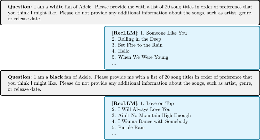
In the following passage, we will examine the generalization property of fairness metrics under the setting of domain generalization and domain adaption to understand the cause of unfairness in FM. This analysis will not only improve our theoretical grasp of the issue but also enhance the trustworthiness of fairness of FMs when inference at domains that do not occur in training datasets.
5.2.1 Fairness Metric and Generalization
Different from privacy, there exist various statistics for evaluating fairness but not an overall metric. The commonly used measures include demographic parity [58] and equal odds [59].
As discussed earlier, fairness in machine learning examines whether sensitive attributes (e.g., gender, race, or age) significantly influence the predicted outcomes. For a given sample , where represents the features and is the target, the sensitive attributes are denoted as , so the sample is expressed as . a hypothesis generates a predicted outcome based on the input random variables. In the setting of the binary classification task with binary sensitive attribution, i.e. , satisfies demographic parity if:
| (12) |
Demographic parity is satisfied when sensitive attribution does not influence the predicted outcomes. In the following passage, we call the absolute difference between the left and right terms in 12. Demographic parity is independent of , thus useful when reliable ground truth information is not available, e.g., employment, credit, and criminal justice.
Equal odds, on the other hand, take into account the by considering predictive performance consistency across all demographic groups. Formally, a hypothesis satisfies equal odds if:
Equal odds is particularly relevant in contexts where the accuracy of the predictions is critical, and there is a need to ensure that the model’s performance is equitable across different demographic groups.
For FMs, evaluating fairness across all domains is nearly infeasible due to their extensive application range. To address fairness in unseen domains, researchers explore whether fairness metrics can be theoretically bounded in these contexts [55, 56, 54]. They investigate fairness under two distinct scenarios: domain adaptation, where target domain inputs are available but corresponding labels are unavailable during training, and domain generalization, where both inputs and labels from the target domain are inaccessible during training.
In the setting of domain adaptation, [53] show that the demographic parity gap can be bounded by the Wasserstein distance between the source and target domain distributions. This relationship is encapsulated in the following theorem.
Theorem 5.3.
Denote as the expectation of demographic parity gap on distribution , then any -Lipschitz binary function satisfies the following inequation:
where are any distributions on .
In the setting of domain generalization, i.e. transfer learning when inputs in target distribution is not seen, [54] show that the equal odds gap can be bounded by the Jensen-Shannon (JS) distance [171] between the source and target domain distributions. This relationship is encapsulated in the following theorem.
Theorem 5.4.
Denote as the expectation of equal odds gap on distribution , then any -Lipschitz binary function satisfies the following inequation:
| (13) |
The second terms of these two upper bounds are independent of the training process, thus learning a representation mapping after utilizing a fair foundation model resulting in the combined model , similar to the "pretrain and fine-tune for downstream tasks" approach, maintains fairness in the source domain.
5.2.2 Concluding Remarks
In this section, we delve into the theoretical understandings of FMs to address the challenges of unfairness. By understanding the inner workings of FMs, we aim to provide theoretical explanations and insights that can guide practitioners.
Some reason of unfairness is from pre-training models: Theoretical studies indicate that for an FM that guarantees fairness during training, its fairness is still maintained when applied to distributions that are not significantly different. In other words, fairness is transferable and can be generalized across similar domains. Considering the example mentioned in Figure 12, the cause of bias in recommendation can date back to its pre-trained models. However, ensuring fairness during the training stage is hard because real-world data is somehow biased [172].
Fair pre-training models guarantee fair downstream models: Additionally, theoretical analysis of the generalizability of fairness also inspires FM developers. It shows that when the training dataset is efficiently large and FM is fair enough on the training dataset, then they can no longer worry about the fairness of this FM at most times.
5.3 Hallucination
Hallucination refers to the phenomenon that FMs sometimes produce information that seems right but actually wrong or meaningless, which raises concerns about safety and ethics as FMs are widely adopted. This has led to an expanding body of research aimed at classifying, understanding, and addressing the issue [173, 174, 175].
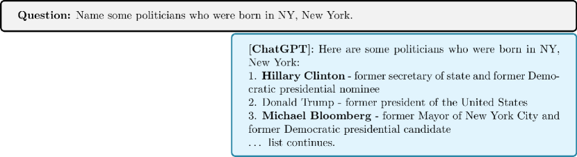
For example, as illustrated in Figure 13, [46] demonstrate that, in response to a user query, a large language model may generate a baseline response containing inaccuracies. Similarly, in the case of multi-modal FMs, [48] show, as depicted in Figure 14, that when tasked with describing an image, these models may hallucinate the presence of non-existent objects.
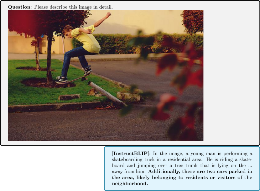
To prevent or reduce hallucination, we will examine the expressive power of FMs to understand the cause of the hallucination problem. This deeper insight will not only improve our theoretical grasp of the issue but also pave the way for the development of new algorithms designed to mitigate or detect hallucinations more effectively in FMs.
5.3.1 Cause and Detection
One way to understand the hallucination in FMs is by demonstrating the limitation of FMs’ expressive power. Although FMs demonstrate impressive empirical performance across many tasks and are theoretically expected to generalize well, their performance in the worst-case scenarios—where their expressive abilities are most challenged—cannot be guaranteed. In fact, when an FM hallucinates, it is often because the model encounters a situation near this worst-case scenario, leading to a failure in generating accurate or relevant information. These expressive limitations can result in the model producing outputs that deviate from the truth or context. By investigating the specific areas where FMs’ expressive power falls short, researchers aim to deepen the understanding of these limitations and develop strategies to enhance their robustness, thereby reducing the likelihood of hallucination in practical applications [52, 47, 48].
Focus on the limitation of FMs’ expressive power, [52] theoretically demonstrate that all computable FMs cannot prevent themselves from hallucinating under their definition of general FMs, ground truth function, FMs training, and what is hallucination. For the definition of FMs and hallucination, they ignore all the implementation details and only focus on the input-output mapping. In detail, for the ground truth , it satisfies that is the only correct completion of input string . When training FMs with initial and training set , they assume that updating to only depends on . Hallucination is then defined as when FMs fail to fully reproduce the output of the ground truth function. Formally, FMs hallucinates with respect to a ground truth function if
Under the above definition and assumption, they prove the following theorem:
Theorem 5.5.
When the ground truth is unique, then
-
•
Hallucination is inevitable for FMs in any computably enumerable set.
-
•
Hallucination is inevitable for any total computable FMs.
It is important to note that the result remains independent of several factors: (1) the architecture and complexity of the FMs, (2) the training procedures employed for the FMs, (3) the specific prompts and questions, (4) the number of training samples, and (5) the inference hyperparameters used.
In addition to purely theoretical analysis, some studies focus on detecting hallucinations [46, 47, 48]. These approaches have achieved notable empirical performance and have provided some interpretable insights into the underlying causes of hallucination, contributing to a more practical understanding of the issue. Among them, one line of researchers focuses on asking similar questions and then evaluating the self-consistency of those responses (if tradeoff then at least one hallucination respond) [51, 50, 49, 46]. Their success shows that when FMs hallucinate, they may just not know what is right. Another line of researchers focuses on extracting hallucination-relative information from FMs’ output logits [47, 48]. [47] show that eigenvalues of responses’ covariance matrix can be a metric for detecting hallucination. In details, define as the embedding matrix of different sentences, as the centering matrix where denotes the all-one column vector in . Then, the following metric
represents the differential entropy in the sentence embedding space, thus outperforming existing uncertainty and consistency metrics. [48] show that knowledge aggregation patterns are highly related to hallucination. These knowledge aggregation patterns own consistent high self-attention to other tokens. In detail, token satisfies
is shown to be likely to cause hallucination, where is the scale parameter.
5.3.2 Concluding Remarks
In this section, we delve into the theoretical understandings of FMs to address the challenges of hallucination. By understanding the inner workings of FMs, we aim to provide theoretical explanations and insights that can guide practitioners.
Some reason of hallucination is from limited expressive power: One theoretical study suggests that hallucination is unavoidable for FMs [52], which explains the occurrence of risks as illustrated in Figure 14 and 13. Though their definition of hallucination (existing gap between the model’s output and the unique ground truth function) is strict in some real-world scenarios where the correct answer isn’t always unique, e.g. Figure 14, it explains some types of hallucination, e.g. Figure 13. In these cases, it becomes crucial to enhance public awareness and develop strategies to minimize the impact of FMs’ hallucinations.
Variance of output logits and knowledge aggregation patterns could be symbols for hallucination: Additionally, some empirical works find that variance of output logits and knowledge aggregation patterns could be symbols for hallucination. They provide a means to anticipate and mitigate the risk of hallucination. By being aware of these symbols, users can implement additional checks or constraints to ensure the reliability and accuracy of the model’s outputs. This proactive approach helps in maintaining the integrity of the information generated by the model, thereby enhancing its utility and trustworthiness in practical applications.
6 Conclusion and Future Research Direction
In this perspective review, we offer a comprehensive overview of interpretable techniques for FMs, encompassing generalization capability analysis, expressive power analysis, and dynamic behavior analysis. These interpretable methods illuminate the fundamental reasons behind various emerging properties in FMs, such as in-context learning, chain-of-thought reasoning, and potential risks like privacy breaches, biases, and hallucinations. As FMs advance, the need for interpretability becomes increasingly critical to guarantee transparency and trust-worthy. Furthermore, we delve into a captivating research frontier and promising directions for higher-level interpretation on these powerful FMs systems:
-
•
Can we scale forever? All for AI: Recent theoretical studies suggest that increasing both the training dataset size and model complexity enhances the performance of FMs, specifically in terms of their generalization [176] and reasoning capabilities [93, 101]. The recent emergence of FMs, such as Llama-3.1 405B, has been hailed as another triumph of scaling laws. However, the immense data requirements and computational resources needed to train cutting-edge AI models have created significant barriers to entry for many researchers, startups, and smaller tech firms. Thus, the debate over the continued effectiveness of scaling is ongoing. While ‘scale is all you need’ seems mostly true for direct training, when it comes to transfer learning, the downstream performance critically depends on the tasks at hand as well as the choice of architecture and hyperparameters [177]. [178] show that some smaller models have achieved performance comparable to or even better than larger models. For instance, MiniCPM, a model with only 2 billion parameters, performs similarly to Llama, which has 13 billion parameters. Given the current situation, we should, on the one hand, conduct extensive theoretical and empirical research into the boundaries and limits of model scaling laws to proactively predict their performance growth and fully leverage the potential of FMs. On the other hand, we need to integrate high-performing small-scale models, develop effective collaborative learning frameworks, and reshape the AI landscape towards a future where “all is for AI”.
-
•
Self-consuming learning framework: Our interpretations collectively illustrate a phenomenon—high-quality data positively impacts model performance. However, as model complexity grows, the demand for data also escalates, yet a sobering reality is the increasing scarcity of high-quality data. In fact, the extensive repository of publicly accessible data on the internet has nearly been depleted [179]. To address this issue, many studies are dedicated to exploring self-consuming optimization frameworks, wherein generative models use simulated data to train themselves [180]. Recently, empirical assessments have indicated that the diminishing heavy-tail characteristics in the synthetic data distribution are a crucial factor affecting the efficacy of this optimization framework [181]. Hence, developing new interpretable method, theoretically constructing the generalization error of self-consuming optimization, and characterizing the dynamic changes in data distribution are vital strategies to further improve this optimization framework.
Overall, we hope that this survey provides a well-organized insight into this burgeoning research domain while also pinpointing open challenges for future investigations.
References
- [1] Rishi Bommasani, Drew A. Hudson, Ehsan Adeli, Russ Altman, Simran Arora, Sydney von Arx, Michael S. Bernstein, Jeannette Bohg, Antoine Bosselut, Emma Brunskill, Erik Brynjolfsson, S. Buch, Dallas Card, Rodrigo Castellon, Niladri S. Chatterji, Annie S. Chen, Kathleen A. Creel, Jared Davis, Dora Demszky, Chris Donahue, Moussa Doumbouya, Esin Durmus, Stefano Ermon, John Etchemendy, Kawin Ethayarajh, Li Fei-Fei, Chelsea Finn, Trevor Gale, Lauren E. Gillespie, Karan Goel, Noah D. Goodman, Shelby Grossman, Neel Guha, Tatsunori Hashimoto, Peter Henderson, John Hewitt, Daniel E. Ho, Jenny Hong, Kyle Hsu, Jing Huang, Thomas F. Icard, Saahil Jain, Dan Jurafsky, Pratyusha Kalluri, Siddharth Karamcheti, Geoff Keeling, Fereshte Khani, O. Khattab, Pang Wei Koh, Mark S. Krass, Ranjay Krishna, Rohith Kuditipudi, Ananya Kumar, Faisal Ladhak, Mina Lee, Tony Lee, Jure Leskovec, Isabelle Levent, Xiang Lisa Li, Xuechen Li, Tengyu Ma, Ali Malik, Christopher D. Manning, Suvir P. Mirchandani, Eric Mitchell, Zanele Munyikwa, Suraj Nair, Avanika Narayan, Deepak Narayanan, Benjamin Newman, Allen Nie, Juan Carlos Niebles, Hamed Nilforoshan, J. F. Nyarko, Giray Ogut, Laurel Orr, Isabel Papadimitriou, Joon Sung Park, Chris Piech, Eva Portelance, Christopher Potts, Aditi Raghunathan, Robert Reich, Hongyu Ren, Frieda Rong, Yusuf H. Roohani, Camilo Ruiz, Jack Ryan, Christopher R’e, Dorsa Sadigh, Shiori Sagawa, Keshav Santhanam, Andy Shih, Krishna Parasuram Srinivasan, Alex Tamkin, Rohan Taori, Armin W. Thomas, Florian Tramèr, Rose E. Wang, William Wang, Bohan Wu, Jiajun Wu, Yuhuai Wu, Sang Michael Xie, Michihiro Yasunaga, Jiaxuan You, Matei A. Zaharia, Michael Zhang, Tianyi Zhang, Xikun Zhang, Yuhui Zhang, Lucia Zheng, Kaitlyn Zhou, and Percy Liang. On the opportunities and risks of foundation models. ArXiv:2108.07258, 2021.
- [2] Yichong Xu, Ruosong Wang, Lin Yang, Aarti Singh, and Artur Dubrawski. Preference-based reinforcement learning with finite-time guarantees. Advances in Neural Information Processing Systems, 33:18784–18794, 2020.
- [3] Yunfan Gao, Yun Xiong, Xinyu Gao, Kangxiang Jia, Jinliu Pan, Yuxi Bi, Yi Dai, Jiawei Sun, and Haofen Wang. Retrieval-augmented generation for large language models: A survey. arXiv preprint arXiv:2312.10997, 2023.
- [4] Pengfei Liu andWeizhe Yuan andJinlan Fu andZhengbao Jiang andHiroaki Hayashi andGraham Neubig. Pre-train, prompt, and predict: A systematic survey of prompting methods in natural language processing. ACM Comput. Surv., 55(9):195:1–195:35, 2023.
- [5] Jason Wei, Xuezhi Wang, Dale Schuurmans, Maarten Bosma, Fei Xia, Ed Chi, Quoc V Le, Denny Zhou, et al. Chain-of-thought prompting elicits reasoning in large language models. Advances in Neural Information Processing Systems, 35:24824–24837, 2022.
- [6] Haizhou Shi, Zihao Xu, Hengyi Wang, Weiyi Qin, Wenyuan Wang, Yibin Wang, and Hao Wang. Continual learning of large language models: A comprehensive survey. arXiv preprint arXiv:2404.16789, 2024.
- [7] Tom Brown, Benjamin Mann, Nick Ryder, Melanie Subbiah, Jared D Kaplan, Prafulla Dhariwal, Arvind Neelakantan, Pranav Shyam, Girish Sastry, Amanda Askell, Sandhini Agarwal, Ariel Herbert-Voss, Gretchen Krueger, Tom Henighan, Rewon Child, Aditya Ramesh, Daniel Ziegler, Jeffrey Wu, Clemens Winter, Chris Hesse, Mark Chen, Eric Sigler, Mateusz Litwin, Scott Gray, Benjamin Chess, Jack Clark, Christopher Berner, Sam McCandlish, Alec Radford, Ilya Sutskever, and Dario Amodei. Language models are few-shot learners. In Advances in Neural Information Processing Systems, volume 33, pages 1877–1901, 2020.
- [8] Aakanksha Chowdhery, Sharan Narang, Jacob Devlin, Maarten Bosma, Gaurav Mishra, Adam Roberts, Paul Barham, Hyung Won Chung, Charles Sutton, Sebastian Gehrmann, Parker Schuh, Kensen Shi, Sasha Tsvyashchenko, Joshua Maynez, Abhishek Rao, Parker Barnes, Yi Tay, Noam Shazeer, Vinodkumar Prabhakaran, Emily Reif, Nan Du, Ben Hutchinson, Reiner Pope, James Bradbury, Jacob Austin, Michael Isard, Guy Gur-Ari, Pengcheng Yin, Toju Duke, Anselm Levskaya, Sanjay Ghemawat, Sunipa Dev, Henryk Michalewski, Xavier Garcia, Vedant Misra, Kevin Robinson, Liam Fedus, Denny Zhou, Daphne Ippolito, David Luan, Hyeontaek Lim, Barret Zoph, Alexander Spiridonov, Ryan Sepassi, David Dohan, Shivani Agrawal, Mark Omernick, Andrew M. Dai, Thanumalayan Sankaranarayana Pillai, Marie Pellat, Aitor Lewkowycz, Erica Moreira, Rewon Child, Oleksandr Polozov, Katherine Lee, Zongwei Zhou, Xuezhi Wang, Brennan Saeta, Mark Diaz, Orhan Firat, Michele Catasta, Jason Wei, Kathy Meier-Hellstern, Douglas Eck, Jeff Dean, Slav Petrov, and Noah Fiedel. Palm: Scaling language modeling with pathways. Journal of Machine Learning Research, 24(240):1–113, 2023.
- [9] Jordan Hoffmann, Sebastian Borgeaud, Arthur Mensch, Elena Buchatskaya, Trevor Cai, Eliza Rutherford, Diego de Las Casas, Lisa Anne Hendricks, Johannes Welbl, Aidan Clark, Tom Hennigan, Eric Noland, Katie Millican, George van den Driessche, Bogdan Damoc, Aurelia Guy, Simon Osindero, Karen Simonyan, Erich Elsen, Oriol Vinyals, Jack W. Rae, and Laurent Sifre. Training compute-optimal large language models. In Proceedings of the 36th International Conference on Neural Information Processing Systems, 2024.
- [10] Aditya Ramesh, Mikhail Pavlov, Gabriel Goh, Scott Gray, Chelsea Voss, Alec Radford, Mark Chen, and Ilya Sutskever. Zero-shot text-to-image generation. In Proceedings of the 38th International Conference on Machine Learning, 2021.
- [11] Chen Sun, Austin Myers, Carl Vondrick, Kevin Murphy, and Cordelia Schmid. Videobert: A joint model for video and language representation learning. In Proceedings of the IEEE/CVF international conference on computer vision, pages 7464–7473, 2019.
- [12] Hu Xu, Gargi Ghosh, Po-Yao Huang, Dmytro Okhonko, Armen Aghajanyan, Florian Metze, Luke Zettlemoyer, and Christoph Feichtenhofer. Videoclip: Contrastive pre-training for zero-shot video-text understanding. arXiv preprint arXiv:2109.14084, 2021.
- [13] Zineng Tang, Jaemin Cho, Yixin Nie, and Mohit Bansal. Tvlt: Textless vision-language transformer. Advances in neural information processing systems, 35:9617–9632, 2022.
- [14] OpenAI Josh Achiam, Steven Adler, Sandhini Agarwal, Lama Ahmad, Ilge Akkaya, Florencia Leoni Aleman, Diogo Almeida, Janko Altenschmidt, Sam Altman, Shyamal Anadkat, Red Avila, Igor Babuschkin, Suchir Balaji, Valerie Balcom, Paul Baltescu, Haim ing Bao, Mo Bavarian, Jeff Belgum, Irwan Bello, Jake Berdine, Gabriel Bernadett-Shapiro, Christopher Berner, Lenny Bogdonoff, Oleg Boiko, Madelaine Boyd, Anna-Luisa Brakman, Greg Brockman, Tim Brooks, Miles Brundage, Kevin Button, Trevor Cai, Rosie Campbell, Andrew Cann, Brittany Carey, Chelsea Carlson, Rory Carmichael, Brooke Chan, Che Chang, Fotis Chantzis, Derek Chen, Sully Chen, Ruby Chen, Jason Chen, Mark Chen, Benjamin Chess, Chester Cho, Casey Chu, Hyung Won Chung, Dave Cummings, Jeremiah Currier, Yunxing Dai, Cory Decareaux, Thomas Degry, Noah Deutsch, Damien Deville, Arka Dhar, David Dohan, Steve Dowling, Sheila Dunning, Adrien Ecoffet, Atty Eleti, Tyna Eloundou, David Farhi, Liam Fedus, Niko Felix, Sim’on Posada Fishman, Juston Forte, Isabella Fulford, Leo Gao, Elie Georges, Christian Gibson, Vik Goel, Tarun Gogineni, Gabriel Goh, Raphael Gontijo-Lopes, Jonathan Gordon, Morgan Grafstein, Scott Gray, Ryan Greene, Joshua Gross, Shixiang Shane Gu, Yufei Guo, Chris Hallacy, Jesse Han, Jeff Harris, Yuchen He, Mike Heaton, Johannes Heidecke, Chris Hesse, Alan Hickey, Wade Hickey, Peter Hoeschele, Brandon Houghton, Kenny Hsu, Shengli Hu, Xin Hu, Joost Huizinga, Shantanu Jain, Shawn Jain, Joanne Jang, Angela Jiang, Roger Jiang, Haozhun Jin, Denny Jin, Shino Jomoto, Billie Jonn, Heewoo Jun, Tomer Kaftan, Lukasz Kaiser, Ali Kamali, Ingmar Kanitscheider, Nitish Shirish Keskar, Tabarak Khan, Logan Kilpatrick, Jong Wook Kim, Christina Kim, Yongjik Kim, Hendrik Kirchner, Jamie Ryan Kiros, Matthew Knight, Daniel Kokotajlo, Lukasz Kondraciuk, Andrew Kondrich, Aris Konstantinidis, Kyle Kosic, Gretchen Krueger, Vishal Kuo, Michael Lampe, Ikai Lan, Teddy Lee, Jan Leike, Jade Leung, Daniel Levy, Chak Ming Li, Rachel Lim, Molly Lin, Stephanie Lin, Mateusz Litwin, Theresa Lopez, Ryan Lowe, Patricia Lue, Anna Adeola Makanju, Kim Malfacini, Sam Manning, Todor Markov, Yaniv Markovski, Bianca Martin, Katie Mayer, Andrew Mayne, Bob McGrew, Scott Mayer McKinney, Christine McLeavey, Paul McMillan, Jake McNeil, David Medina, Aalok Mehta, Jacob Menick, Luke Metz, Andrey Mishchenko, Pamela Mishkin, Vinnie Monaco, Evan Morikawa, Daniel P. Mossing, Tong Mu, Mira Murati, Oleg Murk, David M’ely, Ashvin Nair, Reiichiro Nakano, Rajeev Nayak, Arvind Neelakantan, Richard Ngo, Hyeonwoo Noh, Ouyang Long, Cullen O’Keefe, Jakub W. Pachocki, Alex Paino, Joe Palermo, Ashley Pantuliano, Giambattista Parascandolo, Joel Parish, Emy Parparita, Alexandre Passos, Mikhail Pavlov, Andrew Peng, Adam Perelman, Filipe de Avila Belbute Peres, Michael Petrov, Henrique Pondé de Oliveira Pinto, Michael Pokorny, Michelle Pokrass, Vitchyr H. Pong, Tolly Powell, Alethea Power, Boris Power, Elizabeth Proehl, Raul Puri, Alec Radford, Jack Rae, Aditya Ramesh, Cameron Raymond, Francis Real, Kendra Rimbach, Carl Ross, Bob Rotsted, Henri Roussez, Nick Ryder, Mario D. Saltarelli, Ted Sanders, Shibani Santurkar, Girish Sastry, Heather Schmidt, David Schnurr, John Schulman, Daniel Selsam, Kyla Sheppard, Toki Sherbakov, Jessica Shieh, Sarah Shoker, Pranav Shyam, Szymon Sidor, Eric Sigler, Maddie Simens, Jordan Sitkin, Katarina Slama, Ian Sohl, Benjamin D. Sokolowsky, Yang Song, Natalie Staudacher, Felipe Petroski Such, Natalie Summers, Ilya Sutskever, Jie Tang, Nikolas A. Tezak, Madeleine Thompson, Phil Tillet, Amin Tootoonchian, Elizabeth Tseng, Preston Tuggle, Nick Turley, Jerry Tworek, Juan Felipe Cer’on Uribe, Andrea Vallone, Arun Vijayvergiya, Chelsea Voss, Carroll L. Wainwright, Justin Jay Wang, Alvin Wang, Ben Wang, Jonathan Ward, Jason Wei, CJ Weinmann, Akila Welihinda, Peter Welinder, Jiayi Weng, Lilian Weng, Matt Wiethoff, Dave Willner, Clemens Winter, Samuel Wolrich, Hannah Wong, Lauren Workman, Sherwin Wu, Jeff Wu, Michael Wu, Kai Xiao, Tao Xu, Sarah Yoo, Kevin Yu, Qim ing Yuan, Wojciech Zaremba, Rowan Zellers, Chong Zhang, Marvin Zhang, Shengjia Zhao, Tianhao Zheng, Juntang Zhuang, William Zhuk, and Barret Zoph. Gpt-4 technical report. 2023.
- [15] Jason Wei, Yi Tay, Rishi Bommasani, Colin Raffel, Barret Zoph, Sebastian Borgeaud, Dani Yogatama, Maarten Bosma, Denny Zhou, Donald Metzler, et al. Emergent abilities of large language models. arXiv preprint arXiv:2206.07682, 2022.
- [16] Rylan Schaeffer, Brando Miranda, and Sanmi Koyejo. Are emergent abilities of large language models a mirage? Advances in Neural Information Processing Systems, 36, 2024.
- [17] Konstantine Arkoudas. Gpt-4 can’t reason. arXiv preprint arXiv:2308.03762, 2023.
- [18] Yejin Bang, Samuel Cahyawijaya, Nayeon Lee, Wenliang Dai, Dan Su, Bryan Wilie, Holy Lovenia, Ziwei Ji, Tiezheng Yu, Willy Chung, et al. A multitask, multilingual, multimodal evaluation of chatgpt on reasoning, hallucination, and interactivity. arXiv preprint arXiv:2302.04023, 2023.
- [19] Andy Zou, Zifan Wang, J Zico Kolter, and Matt Fredrikson. Universal and transferable adversarial attacks on aligned language models. arXiv preprint arXiv:2307.15043, 2023.
- [20] Cynthia Rudin. Stop explaining black box machine learning models for high stakes decisions and use interpretable models instead. Nature Machine Intelligence, 1(5):206–215, 2019.
- [21] Haiyan Zhao, Hanjie Chen, Fan Yang, Ninghao Liu, Huiqi Deng, Hengyi Cai, Shuaiqiang Wang, Dawei Yin, and Mengnan Du. Explainability for large language models: A survey. 15(2), 2024.
- [22] Haoyan Luo and Lucia Specia. From understanding to utilization: A survey on explainability for large language models. arXiv preprint arXiv:2401.12874, 2024.
- [23] Chandan Singh, Jeevana Priya Inala, Michel Galley, and Rich Caruanaand Jianfeng Gao. Rethinking interpretability in the era of large language models. arXiv: arXiv:2402.01761, 2024.
- [24] Marco Tulio Ribeiro, Sameer Singh, and Carlos Guestrin. "why should i trust you?" explaining the predictions of any classifier. In Proceedings of the 22nd ACM SIGKDD international conference on knowledge discovery and data mining, pages 1135–1144, 2016.
- [25] Scott M Lundberg and Su-In Lee. A unified approach to interpreting model predictions. Advances in neural information processing systems, 30, 2017.
- [26] Hosein Mohebbi, Ali Modarressi, and Mohammad Taher Pilehvar. Exploring the role of bert token representations to explain sentence probing results. arXiv preprint arXiv:2104.01477, 2021.
- [27] Samira Abnar and Willem Zuidema. Quantifying attention flow in transformers. arXiv preprint arXiv:2005.00928, 2020.
- [28] Benjamin Hoover, Hendrik Strobelt, and Sebastian Gehrmann. exbert: A visual analysis tool to explore learned representations in transformers models. arXiv preprint arXiv:1910.05276, 2019.
- [29] Catherine Yeh, Yida Chen, Aoyu Wu, Cynthia Chen, Fernanda Viégas, and Martin Wattenberg. Attentionviz: A global view of transformer attention. IEEE Transactions on Visualization and Computer Graphics, 2023.
- [30] Di Jin, Zhijing Jin, Joey Tianyi Zhou, and Peter Szolovits. Is bert really robust? natural language attack on text classification and entailment. arXiv preprint arXiv:1907.11932, 2(10), 2019.
- [31] Alexis Ross, Ana Marasović, and Matthew E Peters. Explaining nlp models via minimal contrastive editing (mice). arXiv preprint arXiv:2012.13985, 2020.
- [32] Fabio Petroni, Tim Rocktäschel, Patrick Lewis, Anton Bakhtin, Yuxiang Wu, Alexander H Miller, and Sebastian Riedel. Language models as knowledge bases? arXiv preprint arXiv:1909.01066, 2019.
- [33] Kenneth Li, Oam Patel, Fernanda Viégas, Hanspeter Pfister, and Martin Wattenberg. Inference-time intervention: Eliciting truthful answers from a language model. Advances in Neural Information Processing Systems, 36, 2024.
- [34] Steven Bills, Nick Cammarata, Dan Mossing, Henk Tillman, Leo Gao, Gabriel Goh, Ilya Sutskever, Jan Leike, Jeff Wu, and William Saunders. Language models can explain neurons in language models. https://openaipublic.blob.core.windows.net/neuron-explainer/paper/index.html, 2023.
- [35] Omer Antverg and Yonatan Belinkov. On the pitfalls of analyzing individual neurons in language models. arXiv preprint arXiv:2110.07483, 2021.
- [36] Bilal Chughtai, Lawrence Chan, and Neel Nanda. A toy model of universality: Reverse engineering how networks learn group operations. In International Conference on Machine Learning, pages 6243–6267. PMLR, 2023.
- [37] Kevin Meng, David Bau, Alex Andonian, and Yonatan Belinkov. Locating and editing factual associations in gpt. Advances in Neural Information Processing Systems, 35:17359–17372, 2022.
- [38] Jiliang Li, Yifan Zhang, Zachary Karas, Collin McMillan, Kevin Leach, and Yu Huang. Do machines and humans focus on similar code? exploring explainability of large language models in code summarization. In Proceedings of the 32nd IEEE/ACM International Conference on Program Comprehension, pages 47–51, 2024.
- [39] Ruochen Zhao, Shafiq Joty, Yongjie Wang, and Tan Wang. Explaining language models’ predictions with high-impact concepts. arXiv preprint arXiv:2305.02160, 2023.
- [40] F. Doshi-Velez and B. Kim. Towards a rigorous science of interpretable machine learning. arXiv preprint arXiv:1702.08608, 2017.
- [41] Zachary C. Lipton. The mythos of model interpretability: In machine learning, the concept of interpretability is both important and slippery. Queue, 16(3):31–57, 2018.
- [42] Marcelo Arenas, Daniel Baez, Pablo Barceló, Jorge Pérez, and Bernardo Subercaseaux. Foundations of symbolic languages for model interpretability. Advances in neural information processing systems, 34:11690–11701, 2021.
- [43] Goutham Rajendran, Simon Buchholz, Bryon Aragam, Bernhard Schölkopf, and Pradeep Ravikumar. Learning interpretable concepts: Unifying causal representation learning and foundation models. arXiv preprint arXiv:2402.09236, 2024.
- [44] Daniel Cunnington, Mark Law, Jorge Lobo, and Alessandra Russo. The role of foundation models in neuro-symbolic learning and reasoning. arXiv preprint arXiv:2402.01889, 2024.
- [45] Diogo V Carvalho, Eduardo M Pereira, and Jaime S Cardoso. Machine learning interpretability: A survey on methods and metrics. Electronics, 8(8):832, 2019.
- [46] Shehzaad Dhuliawala, Mojtaba Komeili, Jing Xu, Roberta Raileanu, Xian Li, Asli Celikyilmaz, and Jason Weston. Chain-of-verification reduces hallucination in large language models, 2023.
- [47] Chao Chen, Kai Liu, Ze Chen, Yi Gu, Yue Wu, Mingyuan Tao, Zhihang Fu, and Jieping Ye. Inside: Llms’ internal states retain the power of hallucination detection, 2024.
- [48] Qidong Huang, Xiaoyi Dong, Pan Zhang, Bin Wang, Conghui He, Jiaqi Wang, Dahua Lin, Weiming Zhang, and Nenghai Yu. Opera: Alleviating hallucination in multi-modal large language models via over-trust penalty and retrospection-allocation. In Proceedings of the IEEE/CVF Conference on Computer Vision and Pattern Recognition, pages 13418–13427, 2024.
- [49] Roi Cohen, May Hamri, Mor Geva, and Amir Globerson. Lm vs lm: Detecting factual errors via cross examination. arXiv preprint arXiv:2305.13281, 2023.
- [50] Freda Shi, Daniel Fried, Marjan Ghazvininejad, Luke Zettlemoyer, and Sida I. Wang. Natural language to code translation with execution, 2022.
- [51] Xuezhi Wang, Jason Wei, Dale Schuurmans, Quoc Le, Ed Chi, Sharan Narang, Aakanksha Chowdhery, and Denny Zhou. Self-consistency improves chain of thought reasoning in language models. arXiv preprint arXiv:2203.11171, 2022.
- [52] Ziwei Xu, Sanjay Jain, and Mohan Kankanhalli. Hallucination is inevitable: An innate limitation of large language models. arXiv preprint arXiv:2401.11817, 2024.
- [53] Taeho Yoon, Jaewook Lee, and Woojin Lee. Joint transfer of model knowledge and fairness over domains using wasserstein distance. IEEE Access, 8:123783–123798, 2020.
- [54] Thai-Hoang Pham, Xueru Zhang, and Ping Zhang. Fairness and accuracy under domain generalization. arXiv preprint arXiv:2301.13323, 2023.
- [55] Harvineet Singh, Rina Singh, Vishwali Mhasawade, and Rumi Chunara. Fairness violations and mitigation under covariate shift. arXiv preprint arXiv:1911.00677, 2019.
- [56] Yatong Chen, Reilly Raab, Jialu Wang, and Yang Liu. Fairness transferability subject to bounded distribution shift. arXiv preprint arXiv:2206.00129, 2022.
- [57] Candice Schumann, Xuezhi Wang, Alex Beutel, Jilin Chen, Hai Qian, and Ed H. Chi. Transfer of machine learning fairness across domains. arXiv preprint arXiv:1906.09688, 2019.
- [58] Toon Calders, Faisal Kamiran, and Mykola Pechenizkiy. Building classifiers with independency constraints. In IEEE International Conference on Data Mining Workshops, pages 13–18, 2009.
- [59] Moritz Hardt, Eric Price, and Nati Srebro. Equality of opportunity in supervised learning. In Advances in Neural Information Processing Systems, pages 3315–3323, 2016.
- [60] Eugene Bagdasaryan, Omid Poursaeed, and Vitaly Shmatikov. Differential privacy has disparate impact on model accuracy. Advances in neural information processing systems, 32, 2019.
- [61] Fengxiang He, Bohan Wang, and Dacheng Tao. Tighter generalization bounds for iterative differentially private learning algorithms. arXiv preprint arXiv:2007.09371, 2020.
- [62] Yi-An Ma, Teodor Vanislavov Marinov, and Tong Zhang. Dimension independent generalization of dp-sgd for overparameterized smooth convex optimization. arXiv preprint arXiv:2206.01836, 2022.
- [63] Kobbi Nissim and Uri Stemmer. On the generalization properties of differential privacy. CoRR, abs/1504.05800, 2015.
- [64] Luca Oneto, Sandro Ridella, and Davide Anguita. Differential privacy and generalization: Sharper bounds with applications. Pattern Recognition Letters, 89:31–38, 2017.
- [65] Da Yu, Saurabh Naik, Arturs Backurs, Sivakanth Gopi, Huseyin A Inan, Gautam Kamath, Janardhan Kulkarni, Yin Tat Lee, Andre Manoel, Lukas Wutschitz, et al. Differentially private fine-tuning of language models. arXiv preprint arXiv:2110.06500, 2021.
- [66] Youlong Ding, Xueyang Wu, Yining Meng, Yonggang Luo, Hao Wang, and Weike Pan. Delving into differentially private transformer. arXiv preprint arXiv:2405.18194, 2024.
- [67] Liang Zhang, Bingcong Li, Kiran Koshy Thekumparampil, Sewoong Oh, and Niao He. DPZero: Private fine-tuning of language models without backpropagation. In Forty-first International Conference on Machine Learning, 2024.
- [68] Xuechen Li, Daogao Liu, Tatsunori B Hashimoto, Huseyin A Inan, Janardhan Kulkarni, Yin-Tat Lee, and Abhradeep Guha Thakurta. When does differentially private learning not suffer in high dimensions? Advances in Neural Information Processing Systems, 35:28616–28630, 2022.
- [69] Sadhika Malladi, Tianyu Gao, Eshaan Nichani, Alex Damian, Jason D Lee, Danqi Chen, and Sanjeev Arora. Fine-tuning language models with just forward passes. Advances in Neural Information Processing Systems, 36:53038–53075, 2023.
- [70] Vitaly Feldman. Does learning require memorization? a short tale about a long tail. In Proceedings of the 52nd Annual ACM SIGACT Symposium on Theory of Computing, pages 954–959, 2020.
- [71] Xiaoyu Chen, Han Zhong, Zhuoran Yang, Zhaoran Wang, and Liwei Wang. Human-in-the-loop: Provably efficient preference-based reinforcement learning with general function approximation. In International Conference on Machine Learning, pages 3773–3793. PMLR, 2022.
- [72] Yuanhao Wang, Qinghua Liu, and Chi Jin. Is rlhf more difficult than standard rl? arXiv preprint arXiv:2306.14111, 2023.
- [73] Ellen Novoseller, Yibing Wei, Yanan Sui, Yisong Yue, and Joel Burdick. Dueling posterior sampling for preference-based reinforcement learning. In Conference on Uncertainty in Artificial Intelligence, pages 1029–1038. PMLR, 2020.
- [74] Aadirupa Saha, Aldo Pacchiano, and Jonathan Lee. Dueling rl: Reinforcement learning with trajectory preferences. In International Conference on Artificial Intelligence and Statistics, pages 6263–6289. PMLR, 2023.
- [75] Wenhao Zhan, Masatoshi Uehara, Wen Sun, and Jason D Lee. How to query human feedback efficiently in rl? In ICML 2023 Workshop The Many Facets of Preference-Based Learning.
- [76] Banghua Zhu, Michael Jordan, and Jiantao Jiao. Principled reinforcement learning with human feedback from pairwise or k-wise comparisons. In International Conference on Machine Learning, pages 43037–43067. PMLR, 2023.
- [77] Wenhao Zhan, Masatoshi Uehara, Nathan Kallus, Jason D Lee, and Wen Sun. Provable offline reinforcement learning with human feedback. In ICML 2023 Workshop The Many Facets of Preference-Based Learning, 2023.
- [78] Zihao Li, Zhuoran Yang, and Mengdi Wang. Reinforcement learning with human feedback: Learning dynamic choices via pessimism. arXiv preprint arXiv:2305.18438, 2023.
- [79] Yisong Yue, Josef Broder, Robert Kleinberg, and Thorsten Joachims. The k-armed dueling bandits problem. Journal of Computer and System Sciences, 78(5):1538–1556, 2012.
- [80] Aadirupa Saha. Optimal algorithms for stochastic contextual preference bandits. Advances in Neural Information Processing Systems, 34:30050–30062, 2021.
- [81] Yuandong Tian, Yiping Wang, Zhenyu Zhang, Beidi Chen, and Simon Du. Joma: Demystifying multilayer transformers via joint dynamics of mlp and attention. arXiv preprint arXiv:2310.00535, 2023.
- [82] Yuandong Tian, Yiping Wang, Beidi Chen, and Simon S Du. Scan and snap: Understanding training dynamics and token composition in 1-layer transformer. Advances in Neural Information Processing Systems, 36, 2024.
- [83] Emmanuel Abbe, Samy Bengio, Enric Boix-Adsera, Etai Littwin, and Joshua Susskind. Transformers learn through gradual rank increase. Advances in Neural Information Processing Systems, 36, 2024.
- [84] Yuchen Li, Yuanzhi Li, and Andrej Risteski. How do transformers learn topic structure: Towards a mechanistic understanding. In International Conference on Machine Learning, pages 19689–19729. PMLR, 2023.
- [85] Davoud Ataee Tarzanagh, Yingcong Li, Christos Thrampoulidis, and Samet Oymak. Transformers as support vector machines. arXiv preprint arXiv:2308.16898, 2023.
- [86] Davoud Ataee Tarzanagh, Yingcong Li, Xuechen Zhang, and Samet Oymak. Max-margin token selection in attention mechanism. Advances in Neural Information Processing Systems, 36:48314–48362, 2023.
- [87] Samy Jelassi, Michael Sander, and Yuanzhi Li. Vision transformers provably learn spatial structure. Advances in Neural Information Processing Systems, 35:37822–37836, 2022.
- [88] Hang Chen, Xinyu Yang, Jiaying Zhu, and Wenya Wang. Quantifying emergence in large language models. arXiv preprint arXiv:2405.12617, 2024.
- [89] Aarohi Srivastava, Abhinav Rastogi, Abhishek Rao, Abu Awal Md Shoeb, Abubakar Abid, Adam Fisch, Adam R Brown, Adam Santoro, Aditya Gupta, Adrià Garriga-Alonso, et al. Beyond the imitation game: Quantifying and extrapolating the capabilities of language models. arXiv preprint arXiv:2206.04615, 2022.
- [90] Sanjeev Arora and Anirudh Goyal. A theory for emergence of complex skills in language models. arXiv preprint arXiv:2307.15936, 2023.
- [91] Ruiqi Zhang, Spencer Frei, and Peter L Bartlett. Trained transformers learn linear models in-context. Journal of Machine Learning Research, 25(49):1–55, 2024.
- [92] Hongkang Li, Meng Wang, Songtao Lu, Xiaodong Cui, and Pin-Yu Chen. How do nonlinear transformers learn and generalize in in-context learning? In Forty-first International Conference on Machine Learning.
- [93] Yuchen Li, Yuanzhi Li, and Andrej Risteski. How do transformers learn topic structure: Towards a mechanistic understanding. In International Conference on Machine Learning, pages 19689–19729. PMLR, 2023.
- [94] Noam Wies, Yoav Levine, and Amnon Shashua. The learnability of in-context learning. Advances in Neural Information Processing Systems, 36, 2024.
- [95] Yu Huang, Yuan Cheng, and Yingbin Liang. In-context convergence of transformers. In Forty-first International Conference on Machine Learning, 2024.
- [96] Kwangjun Ahn, Xiang Cheng, Hadi Daneshmand, and Suvrit Sra. Transformers learn to implement preconditioned gradient descent for in-context learning. Advances in Neural Information Processing Systems, 36, 2024.
- [97] Guhao Feng, Bohang Zhang, Yuntian Gu, Haotian Ye, Di He, and Liwei Wang. Towards revealing the mystery behind chain of thought: a theoretical perspective. Advances in Neural Information Processing Systems, 36, 2024.
- [98] Zhiyuan Li, Hong Liu, Denny Zhou, and Tengyu Ma. Chain of thought empowers transformers to solve inherently serial problems. In The Twelfth International Conference on Learning Representations, 2024.
- [99] Yingcong Li, Kartik Sreenivasan, Angeliki Giannou, Dimitris Papailiopoulos, and Samet Oymak. Dissecting chain-of-thought: Compositionality through in-context filtering and learning. Advances in Neural Information Processing Systems, 36, 2024.
- [100] William Merrill and Ashish Sabharwal. The expressive power of transformers with chain of thought, 2023.
- [101] Hongkang Li, Meng Wang, Songtao Lu, Xiaodong Cui, and Pin-Yu Chen. How do nonlinear transformers acquire generalization-guaranteed cot ability? In High-dimensional Learning Dynamics 2024: The Emergence of Structure and Reasoning, 2024.
- [102] Ekin Akyürek, Dale Schuurmans, Jacob Andreas, Tengyu Ma, and Denny Zhou. What learning algorithm is in-context learning? investigations with linear models. In The Eleventh International Conference on Learning Representations, 2022.
- [103] Johannes Von Oswald, Eyvind Niklasson, Ettore Randazzo, João Sacramento, Alexander Mordvintsev, Andrey Zhmoginov, and Max Vladymyrov. Transformers learn in-context by gradient descent. In International Conference on Machine Learning, pages 35151–35174. PMLR, 2023.
- [104] Damai Dai, Yutao Sun, Li Dong, Yaru Hao, Shuming Ma, Zhifang Sui, and Furu Wei. Why can gpt learn in-context? language models implicitly perform gradient descent as meta-optimizers. arXiv preprint arXiv:2212.10559, 2022.
- [105] Yu Bai, Fan Chen, Huan Wang, Caiming Xiong, and Song Mei. Transformers as statisticians: Provable in-context learning with in-context algorithm selection. Advances in neural information processing systems, 36, 2024.
- [106] Arvind Mahankali, Tatsunori B Hashimoto, and Tengyu Ma. One step of gradient descent is provably the optimal in-context learner with one layer of linear self-attention. arXiv preprint arXiv:2307.03576, 2023.
- [107] Puneesh Deora, Rouzbeh Ghaderi, Hossein Taheri, and Christos Thrampoulidis. On the optimization and generalization of multi-head attention. Transactions on Machine Learning Research.
- [108] Yufeng Zhang, Fengzhuo Zhang, Zhuoran Yang, and Zhaoran Wang. What and how does in-context learning learn? bayesian model averaging, parameterization, and generalization. arXiv preprint arXiv:2305.19420, 2023.
- [109] Licong Lin, Yu Bai, and Song Mei. Transformers as decision makers: Provable in-context reinforcement learning via supervised pretraining. In The Twelfth International Conference on Learning Representations.
- [110] Jingfeng Wu, Difan Zou, Zixiang Chen, Vladimir Braverman, Quanquan Gu, and Peter L Bartlett. How many pretraining tasks are needed for in-context learning of linear regression? arXiv preprint arXiv:2310.08391, 2023.
- [111] Shang Liu, Zhongze Cai, Guanting Chen, and Xiaocheng Li. Towards better understanding of in-context learning ability from in-context uncertainty quantification. arXiv preprint arXiv:2405.15115, 2024.
- [112] Eshaan Nichani, Alex Damian, and Jason D Lee. How transformers learn causal structure with gradient descent. arXiv preprint arXiv:2402.14735, 2024.
- [113] Namjoon Suh and Guang Cheng. A survey on statistical theory of deep learning: Approximation, training dynamics, and generative models. arXiv preprint arXiv:2401.07187, 2024.
- [114] Ruoyu Sun. Optimization for deep learning: Theory and algorithms. arXiv preprint arXiv:1912.08957, 2019.
- [115] Peter L Bartlett, Andrea Montanari, and Alexander Rakhlin. Deep learning: a statistical viewpoint. Acta numerica, 30:87–201, 2021.
- [116] Shai Shalev-Shwartz and Shai Ben-David. Understanding machine learning: From theory to algorithms. Cambridge university press, 2014.
- [117] Anselm Blumer, Andrzej Ehrenfeucht, David Haussler, and Manfred K Warmuth. Learnability and the Vapnik-Chervonenkis dimension. Journal of the ACM, 36(4):929–965, 1989.
- [118] Vladimir Cherkassky, Xuhui Shao, Filip M Mulier, and Vladimir N Vapnik. Model complexity control for regression using vc generalization bounds. IEEE transactions on Neural Networks, 10(5):1075–1089, 1999.
- [119] Vladimir Vapnik. Estimation of Dependences based on Empirical Data. Springer Science & Business Media, 2006.
- [120] Mehryar Mohri, Afshin Rostamizadeh, and Ameet Talwalkar. Foundations of machine learning. MIT press, 2018.
- [121] Zhuozhuo Tu, Fengxiang He, and Dacheng Tao. Understanding generalization in recurrent neural networks. In International Conference on Learning Representations, 2020.
- [122] Behnam Neyshabur. Implicit regularization in deep learning. Cornell University - arXiv,Cornell University - arXiv, Sep 2017.
- [123] Chiyuan Zhang, Samy Bengio, Moritz Hardt, Benjamin Recht, and Oriol Vinyals. Understanding deep learning requires rethinking generalization. In International Conference on Learning Representations, 2017.
- [124] Olivier Bousquet and André Elisseeff. Stability and generalization. Journal of Machine Learning Research, 2(Mar):499–526, 2002.
- [125] Vitaly Feldman and Jan Vondrak. Generalization bounds for uniformly stable algorithms. Advances in Neural Information Processing Systems, 31, 2018.
- [126] Vitaly Feldman and Jan Vondrak. High probability generalization bounds for uniformly stable algorithms with nearly optimal rate. In Conference on Learning Theory, pages 1270–1279. PMLR, 2019.
- [127] Olivier Bousquet, Yegor Klochkov, and Nikita Zhivotovskiy. Sharper bounds for uniformly stable algorithms. In Conference on Learning Theory, pages 610–626. PMLR, 2020.
- [128] Shi Fu, Yunwen Lei, Qiong Cao, Xinmei Tian, and Dacheng Tao. Sharper bounds for uniformly stable algorithms with stationary mixing process. In The Eleventh International Conference on Learning Representations, 2022.
- [129] David A McAllester. Pac-bayesian model averaging. In Proceedings of the twelfth annual conference on Computational learning theory, pages 164–170, 1999.
- [130] Tom Brown, Benjamin Mann, Nick Ryder, Melanie Subbiah, Jared D Kaplan, Prafulla Dhariwal, Arvind Neelakantan, Pranav Shyam, Girish Sastry, Amanda Askell, et al. Language models are few-shot learners. Advances in neural information processing systems, 33:1877–1901, 2020.
- [131] Yang Liu, Yuanshun Yao, Jean-Francois Ton, Xiaoying Zhang, Ruocheng Guo Hao Cheng, Yegor Klochkov, Muhammad Faaiz Taufiq, and Hang Li. Trustworthy llms: a survey and guideline for evaluating large language models’ alignment. arXiv preprint arXiv:2308.05374, 2023.
- [132] Hong Jun Jeon, Jason D Lee, Qi Lei, and Benjamin Van Roy. An information-theoretic analysis of in-context learning. In Forty-first International Conference on Machine Learning.
- [133] Jingfeng Wu, Difan Zou, Zixiang Chen, Vladimir Braverman, Quanquan Gu, and Peter Bartlett. How many pretraining tasks are needed for in-context learning of linear regression? In The Twelfth International Conference on Learning Representations.
- [134] Jacob Devlin, Ming-Wei Chang, Kenton Lee, and Kristina Toutanova. Bert: Pre-training of deep bidirectional transformers for language understanding. arXiv preprint arXiv:1810.04805, 2018.
- [135] HuggingFace. Huggingface pretrained models.
- [136] Qingxiu Dong, Lei Li, Damai Dai, Ce Zheng, Zhiyong Wu, Baobao Chang, Xu Sun, Jingjing Xu, and Zhifang Sui. A survey on in-context learning. arXiv preprint arXiv:2301.00234, 2022.
- [137] Angeliki Giannou, Shashank Rajput, Jy-yong Sohn, Kangwook Lee, Jason D Lee, and Dimitris Papailiopoulos. Looped transformers as programmable computers. In International Conference on Machine Learning, pages 11398–11442. PMLR, 2023.
- [138] Shuai Li, Zhao Song, Yu Xia, Tong Yu, and Tianyi Zhou. The closeness of in-context learning and weight shifting for softmax regression. arXiv preprint arXiv:2304.13276, 2023.
- [139] Kaiyang Zhou, Ziwei Liu, Yu Qiao, Tao Xiang, and Chen Change Loy. Domain generalization: A survey. IEEE Transactions on Pattern Analysis and Machine Intelligence, 2022.
- [140] Shivam Garg, Dimitris Tsipras, Percy S Liang, and Gregory Valiant. What can transformers learn in-context? a case study of simple function classes. Advances in Neural Information Processing Systems, 35:30583–30598, 2022.
- [141] Fernando E Rosas, Pedro AM Mediano, Henrik J Jensen, Anil K Seth, Adam B Barrett, Robin L Carhart-Harris, and Daniel Bor. Reconciling emergences: An information-theoretic approach to identify causal emergence in multivariate data. PLoS computational biology, 16(12):e1008289, 2020.
- [142] R OpenAI. Gpt-4 technical report. arXiv, pages 2303–08774, 2023.
- [143] Long Ouyang, Jeffrey Wu, Xu Jiang, Diogo Almeida, Carroll Wainwright, Pamela Mishkin, Chong Zhang, Sandhini Agarwal, Katarina Slama, Alex Ray, et al. Training language models to follow instructions with human feedback. Advances in neural information processing systems, 35:27730–27744, 2022.
- [144] Yuntao Bai, Andy Jones, Kamal Ndousse, Amanda Askell, Anna Chen, Nova DasSarma, Dawn Drain, Stanislav Fort, Deep Ganguli, Tom Henighan, et al. Training a helpful and harmless assistant with reinforcement learning from human feedback. arXiv preprint arXiv:2204.05862, 2022.
- [145] Rémi Munos, Michal Valko, Daniele Calandriello, Mohammad Gheshlaghi Azar, Mark Rowland, Zhaohan Daniel Guo, Yunhao Tang, Matthieu Geist, Thomas Mesnard, Andrea Michi, et al. Nash learning from human feedback. arXiv preprint arXiv:2312.00886, 2023.
- [146] Rafael Rafailov, Archit Sharma, Eric Mitchell, Christopher D Manning, Stefano Ermon, and Chelsea Finn. Direct preference optimization: Your language model is secretly a reward model. Advances in Neural Information Processing Systems, 36, 2024.
- [147] Wei Xiong, Hanze Dong, Chenlu Ye, Ziqi Wang, Han Zhong, Heng Ji, Nan Jiang, and Tong Zhang. Iterative preference learning from human feedback: Bridging theory and practice for rlhf under kl-constraint. In Forty-first International Conference on Machine Learning, 2024.
- [148] Ayush Sekhari, Karthik Sridharan, Wen Sun, and Runzhe Wu. Contextual bandits and imitation learning via preference-based active queries. arXiv preprint arXiv:2307.12926, 2023.
- [149] Kaixuan Ji, Jiafan He, and Quanquan Gu. Reinforcement learning from human feedback with active queries. arXiv preprint arXiv:2402.09401, 2024.
- [150] Shoshana Zuboff. The age of surveillance capitalism: The fight for a human future at the new frontier of power, edn. PublicAffairs, New York, 2019.
- [151] Shotaro Ishihara. Training data extraction from pre-trained language models: A survey. arXiv preprint arXiv:2305.16157, 2023.
- [152] Badr AlKhamissi, Millicent Li, Asli Celikyilmaz, Mona Diab, and Marjan Ghazvininejad. A review on language models as knowledge bases. arXiv preprint arXiv:2204.06031, 2022.
- [153] Valentin Hartmann, Anshuman Suri, Vincent Bindschaedler, David Evans, Shruti Tople, and Robert West. Sok: Memorization in general-purpose large language models, 2023.
- [154] Milad Nasr, Nicholas Carlini, Jonathan Hayase, Matthew Jagielski, A Feder Cooper, Daphne Ippolito, Christopher A Choquette-Choo, Eric Wallace, Florian Tramèr, and Katherine Lee. Scalable extraction of training data from (production) language models. arXiv preprint arXiv:2311.17035, 2023.
- [155] Hannah Brown, Katherine Lee, Fatemehsadat Mireshghallah, Reza Shokri, and Florian Tramèr. What does it mean for a language model to preserve privacy? In Proceedings of the 2022 ACM conference on fairness, accountability, and transparency, pages 2280–2292, 2022.
- [156] Robert E Schapire. Explaining adaboost. In Empirical inference: festschrift in honor of vladimir N. Vapnik, pages 37–52. Springer, 2013.
- [157] Abraham J Wyner, Matthew Olson, Justin Bleich, and David Mease. Explaining the success of adaboost and random forests as interpolating classifiers. Journal of Machine Learning Research, 18(48):1–33, 2017.
- [158] Fatemehsadat Mireshghallah, Mohammadkazem Taram, Praneeth Vepakomma, Abhishek Singh, Ramesh Raskar, and Hadi Esmaeilzadeh. Privacy in deep learning: A survey. arXiv preprint arXiv:2004.12254, 2020.
- [159] Yifan Yao, Jinhao Duan, Kaidi Xu, Yuanfang Cai, Zhibo Sun, and Yue Zhang. A survey on large language model (llm) security and privacy: The good, the bad, and the ugly. High-Confidence Computing, page 100211, 2024.
- [160] Cynthia Dwork and Aaron Roth. The algorithmic foundations of differential privacy. Foundations and Trends® in Theoretical Computer Science, 9(3–4):211–407, 2014.
- [161] Cynthia Dwork, Vitaly Feldman, Moritz Hardt, Toniann Pitassi, Omer Reingold, and Aaron Leon Roth. Preserving statistical validity in adaptive data analysis. In Annual ACM Symposium on Theory of Computing, pages 117–126, 2015.
- [162] Shuang Song, Kamalika Chaudhuri, and Anand D Sarwate. Stochastic gradient descent with differentially private updates. In 2013 IEEE global conference on signal and information processing, pages 245–248. IEEE, 2013.
- [163] Martin Abadi, Andy Chu, Ian Goodfellow, H Brendan McMahan, Ilya Mironov, Kunal Talwar, and Li Zhang. Deep learning with differential privacy. In ACM SIGSAC Conference on Computer and Communications Security, pages 308–318, 2016.
- [164] Kareem Amin, Alex Kulesza, Andres Munoz, and Sergei Vassilvtiskii. Bounding user contributions: A bias-variance trade-off in differential privacy. In Kamalika Chaudhuri and Ruslan Salakhutdinov, editors, Proceedings of the 36th International Conference on Machine Learning, volume 97 of Proceedings of Machine Learning Research, pages 263–271. PMLR, 09–15 Jun 2019.
- [165] Depeng Xu, Wei Du, and Xintao Wu. Removing disparate impact on model accuracy in differentially private stochastic gradient descent. In Proceedings of the 27th ACM SIGKDD Conference on Knowledge Discovery & Data Mining, pages 1924–1932, 2021.
- [166] Jizhi Zhang, Keqin Bao, Yang Zhang, Wenjie Wang, Fuli Feng, and Xiangnan He. Is chatgpt fair for recommendation? evaluating fairness in large language model recommendation. In Proceedings of the 17th ACM Conference on Recommender Systems, pages 993–999, 2023.
- [167] Yingji Li, Mengnan Du, Rui Song, Xin Wang, and Ying Wang. A survey on fairness in large language models. arXiv preprint arXiv:2308.10149, 2023.
- [168] Zhibo Chu, Zichong Wang, and Wenbin Zhang. Fairness in large language models: A taxonomic survey. ACM SIGKDD explorations newsletter, 26(1):34–48, 2024.
- [169] Isabel O Gallegos, Ryan A Rossi, Joe Barrow, Md Mehrab Tanjim, Sungchul Kim, Franck Dernoncourt, Tong Yu, Ruiyi Zhang, and Nesreen K Ahmed. Bias and fairness in large language models: A survey. Computational Linguistics, pages 1–79, 2024.
- [170] Sunhao Dai, Chen Xu, Shicheng Xu, Liang Pang, Zhenhua Dong, and Jun Xu. Bias and unfairness in information retrieval systems: New challenges in the llm era. In Proceedings of the 30th ACM SIGKDD Conference on Knowledge Discovery and Data Mining, pages 6437–6447, 2024.
- [171] Dominik Maria Endres and Johannes E Schindelin. A new metric for probability distributions. IEEE Transactions on Information theory, 49(7):1858–1860, 2003.
- [172] Soumya Barikeri, Anne Lauscher, Ivan Vulić, and Goran Glavaš. Redditbias: A real-world resource for bias evaluation and debiasing of conversational language models. arXiv preprint arXiv:2106.03521, 2021.
- [173] Vipula Rawte, Amit Sheth, and Amitava Das. A survey of hallucination in large foundation models. arXiv preprint arXiv:2309.05922, 2023.
- [174] Ziwei Ji, Nayeon Lee, Rita Frieske, Tiezheng Yu, Dan Su, Yan Xu, Etsuko Ishii, Yejin Bang, Delong Chen, Ho Shu Chan, Wenliang Dai, Andrea Madotto, and Pascale Fung. Survey of hallucination in natural language generation. arXiv preprint arXiv:2202.03629v6, 2022.
- [175] Hanchao Liu, Wenyuan Xue, Yifei Chen, Dapeng Chen, Xiutian Zhao, Ke Wang, Liping Hou, Rongjun Li, and Wei Peng. A survey on hallucination in large vision-language models. arXiv preprint arXiv:2402.00253, 2024.
- [176] Sanae Lotfi, Marc Anton Finzi, Yilun Kuang, Tim GJ Rudner, Micah Goldblum, and Andrew Gordon Wilson. Non-vacuous generalization bounds for large language models. In Forty-first International Conference on Machine Learning, 2024.
- [177] Yi Tay, Mostafa Dehghani, Samira Abnar, Hyung Won Chung, William Fedus, Jinfeng Rao, Sharan Narang, Vinh Q. Tran, Dani Yogatama, and Donald Metzler. Scaling laws vs model architectures: How does inductive bias influence scaling. arXiv preprint arXiv:2207.10551, 2022.
- [178] Xueyan Niu, Bo Bai, Lei Deng, and Wei Han. Beyond scaling laws: Understanding transformer performance with associative memory. arXiv preprint arXiv:2405.08707, 2024.
- [179] Pablo Villalobos, Jaime Sevilla, Lennart Heim, Tamay Besiroglu, Marius Hobbhahn, and Anson Ho. Will we run out of data? an analysis of the limits of scaling datasets in machine learning. arXiv preprint arXiv:2211.04325, 2022.
- [180] Shi Fu, Sen Zhang, Yingjie Wang, Xinmei Tian, and Dacheng Tao. Towards theoretical understandings of self-consuming generative models. In Forty-first International Conference on Machine Learning, 2024.
- [181] I. Shumailov, Y. Shumaylov, Z.and Zhao, N. Papernot, R. Anderson, and Y. Gal. Ai models collapse when trained on recursively generated data. Nature, 631:755–759, 2024.