Abstract

Modeling complex systems that evolve toward equilibrium distributions is important in various physical applications, including molecular dynamics and robotic control. These systems often follow the stochastic gradient descent of an underlying energy function, converging to stationary distributions around energy minima. The local covariance of these distributions is shaped by the energy landscape’s curvature, often resulting in anisotropic characteristics. While flow-based generative models have gained traction in generating samples from equilibrium distributions in such applications, they predominately employ isotropic conditional probability paths, limiting their ability to capture such covariance structures.

In this paper, we introduce Hessian-Informed Flow Matching (HI-FM), a novel approach that integrates the Hessian of an energy function into conditional flows within the flow matching framework. This integration allows HI-FM to account for local curvature and anisotropic covariance structures. Our approach leverages the linearization theorem from dynamical systems and incorporates additional considerations such as time transformations and equivariance. Empirical evaluations on the MNIST and Lennard-Jones particles datasets demonstrate that HI-FM improves the likelihood of test samples.

1 Introduction

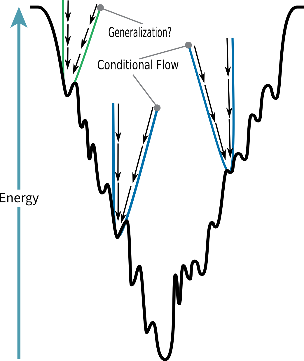
Figure 1: A schematic of HI-FM, where conditional flows are defined via a linear approximation of the dynamics of equilibrium (via the Hessian). These approximations incorporate the underlying anisotropy of the system, which may lead to generalization to unseen parts of the energy landscape (green). These flows are radially unbounded, flowing faster than plateauing potentials (e.g. Lennard-Jones).

Generative modeling is a central problem in machine learning, where a primary goal is to learn a model that can generate samples from a complex target distribution. In recent years, flow-based generative models, such as diffusion [Song et al., 2020] and flow matching Lipman et al. [2022] have come to the forefront of deep generative modeling, with success ranging from image generation Rombach et al. [2021] to biology applications [Abramson et al., 2024] to robotic applications [Chi et al., 2024].

In physical systems, one is often interested in identifying states in which the system is at equilibrium. For instance, in biology, different conformations in protein folding [Abramson et al., 2024] and drug binding [Corso et al., 2023] represent minima of a potential energy function. Similarly, in robotics, stable formations of robotics swarms [Sun et al., 2017] or stable grasps of robotic manipulators [Jiang et al., 2021], often represent the minimization of some energy function, e.g. a Lyapunov function [La Salle, 1966]. And generally, in statistical physics, it is of interest to identify energy minimizing states that, in turn, are likelihood maximizing states.

The states of these systems are often considered to evolve according to the gradient descent of some potential function. These dynamics eventually converge to a stationary distribution (about one of the energy’s minima), whose curvature is determined by the local curvature of the energy landscape, and is often anisotropic. Despite that both flow matching and the physical systems whose equilibrium distribution they often seek to sample, are based on dynamical systems, discrepancies between them remain: most diffusion and flow matching models only employ isotropic probability paths, ignoring potentially important aspects of the underlying physics.

Properly taking into account the anisotropy inherent to a given system is important for the following reasons. It captures the curvature of the energy landscape which could help models better understand the landscape’s curvature in unseen parts of the ambient space. It captures different spatiotemporal timescales, i.e. dynamics converge slower in certain directions and faster in others. It captures the inherent invariances of the energy landscape (and the equivariances of its gradient descent), e.g. the Hessian of an energy function that is invariant to 3D translations and rotations will have at least 6 zero eigenvalues, such that transformations along their corresponding eigenvectors will have no effect.

In this work we construct anisotropic conditional flows that incorporate local energy landscape information via the Hessian of an energy function. We base this incorporation of the Hessian on the well-known linearization theorem from dynamical systems. We then show how these flows can be transformed so that they are amenable to likelihood computation, via the construction of “interpolant dynamics” that follows the distribution of the data flow. In doing so, we make several connections between flow matching, stochastic stability, topological conjugacy, group invariance, and robotic formation control.

2 Related Work

Flow-based deep generative models have gained significant attention for their ability to model complex distributions in various domains. Notably, diffusion models [Song et al., 2020] have achieved state-of-the-art results in image generation tasks [Dhariwal and Nichol, 2021] and have been extended to applications such as structural biology [Corso et al., 2023, Yim et al., 2023b, Ketata et al., 2023] and video generation [Ho et al., 2022, Blattmann et al., 2023, Esser et al., 2023], incorporating latent representations [Vahdat et al., 2021, Blattmann et al., 2023] and geometric priors [Bortoli et al., 2022, Dockhorn et al., 2021].

Flow Matching (FM) models [Lipman et al., 2022] have been proposed as an alternative to diffusion models, offering faster training and sampling while maintaining competitive performance. Relying on continuous normalizing flows (CNFs) [Chen et al., 2018], FM models generalize diffusion models, as demonstrated by the existence of the probability flow ODE that induces the same marginal probability density function (PDF) as the SDE of diffusion models [Song et al., 2020]. FM models have found applications in structural biology [Yim et al., 2023a, Bose et al., 2023], media [Le et al., 2023, Liu et al., 2023], and have been extended in various fundamental ways [Tong et al., 2023, Pooladian et al., 2023, Shaul et al., 2023, Chen and Lipman, 2023, Klein et al., 2023].

In modeling physically stable states, such as molecular conformations, several works have leveraged the connection between the score function and Boltzmann distributions, i.e., $\nabla_{\boldsymbol{x}}\log(p(\boldsymbol{x},t))=-\nabla_{\boldsymbol{x}}V(\boldsymbol{x},t)$ where $V$ is a scalar energy function. For instance, Zaidi et al. [2022] highlighted the equivalence between denoising score matching [Vincent, 2011] and force-field learning. This concept was extended in Feng et al. [2023] to incorporate off-equilibrium data and neural network gradient fields. Other works [Shi et al., 2021, Luo et al., 2021] have learned neural network gradient fields to model pseudo-force fields, subsequently using them to sample energy-minimizing molecular conformations via annealed Langevin dynamics [Song and Ermon, 2019].

While these approaches utilize the gradient of the energy function, most flow-based generative modeling approaches assume isotropic covariance structures and may not fully capture the anisotropic characteristics arising from the curvature of the energy landscape Only a few approaches have considered non-isotropic distributions [Yu et al., 2024, Singhal et al., 2024], but these do not deal with Hessians. Dehmamy et al. [2024] have considered gradient flows defined by Hessians, but not for flow-based generative models. Modeling anisotropic covariance structures requires accounting for the Hessian of the energy function, which provides second-order information about the local curvature. In contrast to all of the above works, we consider anisotropic conditional flows in flow matching using Hessian of the energy, drawing various connections to dynamical system theory.

3 Preliminaries

In this paper, we assume that we have a dataset $\mathcal{D}\subset\mathcal{X}$ existing in an ambient space $\mathcal{X}\subseteq\mathbb{R}^{n}$ that we assume to be described by a latent distribution $q\in\mathcal{P}(\mathcal{X})$ in the space of distributions with support on $\mathcal{X}$, such that $\mathcal{D}\subset\mathrm{supp}(q)$. Our goal is to generate new samples from the latent PDF $q$.

One way to accomplish this goal is to model the distribution explicitly; however, this comes with the burden of ensuring it has a suitable normalizing constant, i.e. such that $\int_{\mathcal{X}}q(\boldsymbol{x})\mathrm{d}\boldsymbol{x}=1$, which is often intractable. Another way to accomplish this goal is to model a vector field $\boldsymbol{v}:\mathcal{X}\times\mathbb{R}_{\geq 0}\to\mathbb{R}^{n}$, which in the context of the continuity equation and flow equation,

Continuity: $$\quad\frac{\partial p(\boldsymbol{x},t)}{\partial t}=-\nabla_{\boldsymbol{x}}\cdot\left(p(\boldsymbol{x},t)\boldsymbol{v}(\boldsymbol{x},t)\right)$$ (1)

Flow: $$\quad\frac{\mathrm{d}\boldsymbol{\phi}(\boldsymbol{x},t)}{\mathrm{d}t}=\boldsymbol{v}\left(\boldsymbol{\phi}(\boldsymbol{x},t),t\right),$$ (2)

offers the ability to sample the push-forward $p(\boldsymbol{x},T)$ of the base distribution $p(\boldsymbol{x},0)$ via the flow $\boldsymbol{\phi}(\boldsymbol{x},T)$. Importantly, the vector field has no inherent restrictions, allowing for more expressivity in its architecture.

Flow matching employs the latter approach, where we assume that there exists a marginal probability path $p(\boldsymbol{x},t)$ that takes us from a simple base distribution, e.g. $p(\cdot,0)=\mathcal{N}(\boldsymbol{0},\boldsymbol{I})$, to the data distribution $p(\boldsymbol{x},T)=q(\boldsymbol{x})$. As a consequence of the continuity equation, this assumption implies the existence of a transporting marginal vector field $\boldsymbol{v}(\boldsymbol{x},t)$. We then assume that we can construct the marginal probability path with a mixture of conditional probability paths $p_{1}(\boldsymbol{x},t\mid\boldsymbol{x}_{1})$ and conditional vector fields $\boldsymbol{v}_{1}(\boldsymbol{x},t\mid\boldsymbol{x}_{1})$:

$$p(\boldsymbol{x},t)= \int_{\mathcal{X}}p_{1}(\boldsymbol{x},t\mid\boldsymbol{x}_{1})q(\boldsymbol{x}_{1})\mathrm{d}\boldsymbol{x}_{1},$$ (3)

$$\boldsymbol{v}(\boldsymbol{x},t)= \frac{1}{p(\boldsymbol{x},t)}\int_{\mathcal{X}}\boldsymbol{v}_{1}(\boldsymbol{x},t\mid\boldsymbol{x}_{1})p_{1}(\boldsymbol{x},t\mid\boldsymbol{x}_{1})q(\boldsymbol{x}_{1})\mathrm{d}\boldsymbol{x}_{1}.$$ (4)

Lipman et al. [2022] showed that we can train a model $\boldsymbol{v}_{\theta}(\boldsymbol{x},t)$ to match a convex combination of conditional vector fields:

$$L_{\text{FM}}(\theta)= \underset{\begin{subarray}{c}t\sim\mathcal{U}[0,T]\\ \boldsymbol{x}_{1}\sim q(\boldsymbol{x}_{1})\\ \boldsymbol{x}\sim p_{1}(\boldsymbol{x},t\mid\boldsymbol{x}_{1})\end{subarray}}{\mathbb{E}}\lVert\boldsymbol{v}_{\theta}(\boldsymbol{x},t)-\boldsymbol{v}_{1}(\boldsymbol{x},t\mid\boldsymbol{x}_{1})\rVert^{2}_{2}$$ (5)

$$= \underset{\begin{subarray}{c}t\sim\mathcal{U}[0,T]\\ \boldsymbol{x}\sim p(\boldsymbol{x},t)\end{subarray}}{\mathbb{E}}\lVert\boldsymbol{v}_{\theta}(\boldsymbol{x},t)-\boldsymbol{v}(\boldsymbol{x},t)\rVert^{2}_{2}+\text{Const}.$$ (6)

Notably, due to the existence of the probability flow vector field [Song et al., 2020, Maoutsa et al., 2020]

$$\boldsymbol{v}(\boldsymbol{x},t)=\boldsymbol{f}(\boldsymbol{x},t)-\frac{1}{2}\nabla_{\boldsymbol{x}}\cdot\boldsymbol{g}(\boldsymbol{x},t)^{2}-\frac{1}{2}\boldsymbol{g}(\boldsymbol{x},t)^{2}\nabla_{\boldsymbol{x}}\ln(p(\boldsymbol{x},t)),$$ (7)

which corresponds to a stochastic differential equation (SDE) of the form

$$\mathrm{d}\boldsymbol{x}=\boldsymbol{f}(\boldsymbol{x},t)\mathrm{d}t+\boldsymbol{g}(\boldsymbol{x},t)\mathrm{d}\boldsymbol{w}$$ (8)

where $\boldsymbol{f}:\mathcal{X}\times\mathbb{R}_{\geq 0}\to\mathbb{R}^{n}$ and $\boldsymbol{g}:\mathcal{X}\times\mathbb{R}_{\geq 0}\to\mathbb{R}^{n\times n}$ are know as drift and diffusion respectively, the flow-matching framework also applies to diffusion probability paths, where plugging the probability flow vector field Eq. 7 into the continuity equation yields the well-known Fokker-Planck-Kolmogorov equation. Conveniently, when the SDE is linear, its score has a closed-form $\nabla_{\boldsymbol{x}}\ln(p(\boldsymbol{x},t))=-\boldsymbol{\Sigma}(t)^{-1}(\boldsymbol{x}-\boldsymbol{\mu}(t))$ [Lindquist and Picci, 1979, Hyvärinen, 2005], where the mean $\boldsymbol{\mu}(t)$ and covariance $\boldsymbol{\Sigma}(t)$ are straightforward to compute [Särkkä and Solin, 2019, Section 6.2].

4 Main Result

In this section we will disect our ambient space into two subspaces: a data space $\mathcal{Y}\subseteq\mathbb{R}^{n-1}$ and an interpolant space $\mathcal{Z}\subseteq\mathbb{R}$, such that $\mathcal{X}=\mathcal{Y}\times\mathcal{Z}$. In Section 4.1, we will describe the dynamics of the data $\boldsymbol{y}\in\mathcal{Y}$, and in Section 4.1, we will describe the dynamics of the interpolant $z\in\mathcal{Z}$.

4.1 Toplogically Conjugate Flows

We will now assume that we are working with data $\boldsymbol{y}\in\mathcal{Y}$ that approximately represent the minima of an energy function $V:\mathcal{Y}\to\mathbb{R}_{\geq 0}$ that defines a stationary Boltzmann-like distribution

$$p(\boldsymbol{y},\infty)=\frac{\exp(-V(\boldsymbol{y}))}{Z}$$ (9)

which implies $\nabla_{\boldsymbol{y}}\ln(p(\boldsymbol{y},\infty))=-\nabla_{\boldsymbol{y}}V(\boldsymbol{y})$, where the descent of the energy $V(\boldsymbol{y})$ corresponds to the ascent of the likelihood $p(\boldsymbol{y},\infty)$. With this in mind, we can formulate a SDE of the form

$$\mathrm{d}\boldsymbol{y}=-\nabla_{\boldsymbol{y}}V(\boldsymbol{y})\mathrm{d}t+\boldsymbol{B}\mathrm{d}\boldsymbol{w}\quad\text{s.t.}\quad\boldsymbol{B}\in\mathbb{R}^{(n-1)\times(n-1)}_{\geq 0},$$ (10)

where $\boldsymbol{B}$ is a positive semidefinite diffusion matrix accounting for the approximate nature of the data $\boldsymbol{y}$. Due to the positive semidefinitness of $V(\boldsymbol{y})$, stochastic stability to the set of energy minima $\mathcal{B}_{1}$ is guaranteed via the infinitesimal generator $\mathcal{L}V$:

$$\mathcal{L}V(\boldsymbol{y})=-\nabla_{\boldsymbol{y}}V(\boldsymbol{y})^{2}+\frac{1}{2}\mathrm{tr}\left(\nabla_{\boldsymbol{y}}^{2}V(\boldsymbol{y})\boldsymbol{B}^{2}\right),$$ (11)

$$\mathcal{B}_{0}=\left\{\boldsymbol{y}\mid\mathcal{L}V(\boldsymbol{y})\leq 0\right\},\quad\mathcal{B}_{1}=\left\{\boldsymbol{y}\mid\mathcal{L}V(\boldsymbol{y})=0\right\}$$ (12)

such that $\boldsymbol{y}_{0}\in\mathcal{B}_{0}\implies\boldsymbol{\phi}(\boldsymbol{y}_{0},\infty)\in\mathcal{B}_{1}$ almost surely [Mao, 1999, Corollary 4.1], where $\mathcal{B}_{1}$ will locally resemble an ellipsoid determined by magnitude of the stochastic fluctuations due to the diffusion matrix $\boldsymbol{B}$.

We will now argue that the stationary distribution can be locally described by a Gaussian. Consider that we take the diffusion to be zero $\boldsymbol{B}=\boldsymbol{0}$. Then the SDE becomes an ordinary differential equation (ODE) $\dot{\boldsymbol{y}}=-\nabla_{\boldsymbol{y}}V(\boldsymbol{y})$. Then the well-known linearization theorem (or Hartman-Grobman theorem) says that the dynamics in a neighborhood $\mathcal{B}\supseteq\{\boldsymbol{y}_{1}\}$ of an equilibrium point $\boldsymbol{y}_{1}$ are locally topologically conjugate to its linearization [Khalil, 2002], that is

$$-\nabla_{\boldsymbol{y}}V(\boldsymbol{y}_{1})=\boldsymbol{0}\implies-\nabla_{\boldsymbol{y}}V(\boldsymbol{y})\approx-\boldsymbol{A}(\boldsymbol{y}-\boldsymbol{y}_{1})$$ (13)

for all $\boldsymbol{y}\in\mathcal{B}$, where $\boldsymbol{A}=\nabla_{\boldsymbol{y}}^{2}V(\boldsymbol{y}_{1})$ is the Hessian of the energy function evaluated at $\boldsymbol{y}_{1}$. This holds when the Hessian is hyperbolic, that is when its nullspace is trivial $\mathrm{null}(\boldsymbol{A})=\{\boldsymbol{0}\}$ (no zero eigenvalues). We will address the non-hyperbolic case in the Section 4.3.

With the deterministic part of the dynamics at hand, we can incorporate stochasticity $\boldsymbol{B}$ back into the dynamics

$$\mathrm{d}\boldsymbol{y}=-\boldsymbol{A}(\boldsymbol{y}-\boldsymbol{y}_{1})\mathrm{d}t+\boldsymbol{B}\boldsymbol{w}\quad\text{s.t.}\quad\begin{aligned} \boldsymbol{A}=&\boldsymbol{P}\mathrm{diag}[\alpha_{i}]\boldsymbol{P}^{\top}\\ \boldsymbol{B}=&\boldsymbol{P}\mathrm{diag}[\beta_{i}]\boldsymbol{P}^{\top}\end{aligned}$$ (14)

where the choice of commuting $\boldsymbol{A}$ and $\boldsymbol{B}$ (such that $\boldsymbol{P}$ is the eigenvector matrix of $\boldsymbol{A}$) allows us to obtain the mean $\boldsymbol{\mu}(t)$ and covariance $\boldsymbol{\Sigma}(t)$ in closed-form, assuming $\boldsymbol{\mu}(0)=\boldsymbol{y}_{0}$ and $\boldsymbol{\Sigma}(0)=\boldsymbol{P}\mathrm{diag}[\sigma_{i}]\boldsymbol{P}^{\top}$:

$$\boldsymbol{\mu}_{y}(t)= \boldsymbol{y}_{1}+\boldsymbol{P}\mathrm{diag}\left[e^{-\alpha_{i}t}\right]\boldsymbol{P}^{\top}(\boldsymbol{y}_{0}-\boldsymbol{y}_{1})$$ (15)

$$\boldsymbol{\Sigma}_{y}(t)= \boldsymbol{P}\mathrm{diag}\left[\frac{\beta_{i}^{2}}{2\alpha_{i}}+e^{-2\alpha t}\left(\sigma_{i}-\frac{\beta_{i}^{2}}{2\alpha_{i}}\right)\right]\boldsymbol{P}^{\top}.$$ (16)

The probability flow vector field is then straightforwardly obtained as

$$\boldsymbol{v}_{y}(\boldsymbol{y},t)=-\boldsymbol{A}(\boldsymbol{y}-\boldsymbol{y}_{1})+\frac{1}{2}\boldsymbol{B}^{2}\boldsymbol{\Sigma}_{y}(t)^{-1}(\boldsymbol{y}-\boldsymbol{\mu}_{y}(t)),$$ (17)

where $\boldsymbol{\Sigma}_{y}(t)^{-1}$ is easily obtained by the reciprocal of its eigenvalues. With these equations, we can then perform flow matching for a chosen $T\in\mathbb{R}_{\geq 0}$. However, as the topological conjugacy of the abovementioned linear flows occurs as $T\to\infty$ due to the above stochastic stability, it is not clear how to practically do flow matching. Moreover, it is unclear what the integration window would be for computing the likelihood of data under the model. We will address this in the next section.

4.2 Interpolant Dynamics

To render a consistent integration window for flow matching and likelihood computation, we consider that time in the context of flow matching is just a quantity used to signify where we are between the initial distribution and final distribution. A time-varying vector field $\boldsymbol{v}:\mathcal{Y}\times\mathbb{R}_{\geq 0}\to\mathbb{R}^{n-1}$ may be interpreted as a time-invariant vector field $\boldsymbol{v}:\mathcal{Y}\times\mathcal{Z}\to\mathbb{R}^{n}$ such that $v(\boldsymbol{y},z)=[\cdot,1]$, where the dynamics of the interpolant state $z\in\mathcal{Z}=\mathbb{R}_{\geq 0}$ is simply one. To see this, consider the optimal-transport conditional vector field [Lipman et al., 2022] with $\boldsymbol{x}=[\boldsymbol{y},z]\in\mathcal{X}=\mathcal{Y}\times\mathcal{Z}$,

$$\boldsymbol{v}_{y}(\boldsymbol{y},z\mid\boldsymbol{x}_{1})=\frac{\boldsymbol{y}_{1}-(1-\sigma_{\min})\boldsymbol{y}}{1-(1-\sigma_{\min})z},\quad v_{z}(\boldsymbol{y},z\mid\boldsymbol{x}_{1})=1,$$ (18)

with mean $\boldsymbol{\mu}_{y}(t)=z\boldsymbol{y}_{1}$ and covariance $\boldsymbol{\Sigma}_{y}(t)=\left(1-(1-\sigma_{\min})z\right)^{2}\boldsymbol{I}$. With this flow, we can match flows over $z\in[0,1]$ as usual.

The “straightness” of the optimal transport flow helps to make training and inference faster. Along the same lines, we consider using an interpolant state that varies at the same rate as the topologically conjugate flows in the previous section. To do this, we model the interpolant state as a deterministic system the “follows” the data state via its distance $d(t)\in\mathbb{R}_{\geq 0}$ to its stationary distribution:

$$\mu_{z}(t)=1-\left(\frac{d(t)}{d(0)}\right)^{\kappa}\quad\text{s.t.}\quad d(\infty)=0,\quad\kappa\in\mathbb{R}_{\geq 0}.$$ (19)

Concretely, $d(t)$ should originate from a probabilistic distance metric (e.g. Wasserstein distance) satisfying the usual axioms, which is available in closed-form for Gaussian probability paths. In this paper, we consider the distance from the intermediate mean to the stationary mean, which supplies us with an upper-bound for the worst-case distance [Kågström, 1977, Moler and Van Loan, 1978],

$$d(t)=\lVert\boldsymbol{\mu}_{y}(t)-\boldsymbol{\mu}_{y}(\infty)\rVert_{2}\leq e^{-\alpha_{\min}t}\lVert\boldsymbol{y}_{0}-\boldsymbol{y}_{1}\rVert_{2},$$ (20)

where $\alpha_{\min}$ is the minimum non-zero eigenvalue of $\boldsymbol{A}$. With this metric, the interpolant dynamics become

$$\mu_{z}(t)=1-e^{-\kappa\alpha_{\min}t},\quad v_{z}(z,t)=-\kappa\alpha_{\min}(z-1).$$ (21)

Now, to achieve a consistent window for sampling, we can invert the mean $\mu_{z}(t)$ of the interpolant state to get the data state’s probability path with respect to the interpolant state, as well as their vector fields with respect to time:

$$\begin{gathered}\boldsymbol{\mu}_{y}(z)=\boldsymbol{y}_{1}+\boldsymbol{P}\mathrm{diag}\left[(1-z)^{\frac{\alpha_{i}}{\kappa\alpha_{\min}}}\right]\boldsymbol{P}^{\top}(\boldsymbol{y}_{0}-\boldsymbol{y}_{1})\\ \boldsymbol{\Sigma}_{y}(z)=\boldsymbol{P}\mathrm{diag}\left[\frac{\beta_{i}^{2}}{2\alpha_{i}}+(1-z)^{\frac{2\alpha_{i}}{\kappa\alpha_{\min}}}\left(\sigma_{i}-\frac{\beta_{i}^{2}}{2\alpha_{i}}\right)\right]\boldsymbol{P}^{\top}.\end{gathered}$$ (22)

Note that the upper bound in Eq. 20 is needed to access this invertibility. We will explore “multidimensional” interpolants [Lee and Lee, 2024] to relieve this need in future work. Now, for the conditional vector fields, we are presented with two options:

1. Infinite: Learn from $\boldsymbol{v}(\boldsymbol{y},z\mid\boldsymbol{y}_{1})=[\boldsymbol{v}_{y}(\boldsymbol{y},z\mid\boldsymbol{y}_{1}),v_{z}(\boldsymbol{y},z\mid\boldsymbol{y}_{1})]$, which has stability from Eq. 11 but does not have a consistent integration window $t\in[0,\infty)$.

2. Finite: Learn from $\boldsymbol{v}(\boldsymbol{y},z\mid\boldsymbol{y}_{1})=[\boldsymbol{v}_{y}(\boldsymbol{y},z\mid\boldsymbol{y}_{1})/v_{z}(\boldsymbol{y},z\mid\boldsymbol{y}_{1}),1]$, which does not have stability from Eq. 11 but does have a consistent integration window $t\in[0,1]$. Note that this vector field produces the probability path in Eq. 22.

In either case, assuming that our architecture outputs both $\boldsymbol{v}_{y}$ and $\boldsymbol{v}_{z}$, we can apply the finite transformation above to compute the likelihood of data as in [Lipman et al., 2022, App. C] with $t\in[0,1]$.

4.3 Invariant Energy

Null Space Dynamics

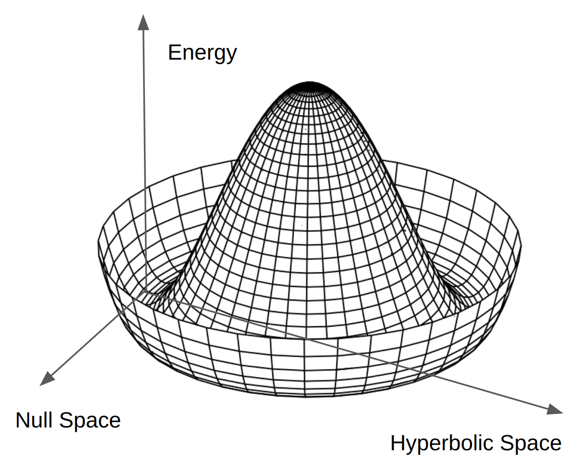
Figure 2: A depiction of the Eigen subspaces of the Hessian of a group-invariant energy function. This energy function is invariant to rotations in $\mathrm{SO}(2)$.

Now we will consider the case that the Hessian $\boldsymbol{A}$ has a non-trivial nullspace $\mathrm{null}(\boldsymbol{A})\neq\{\boldsymbol{0}\}$ (some zero eigenvalues). In this case, the linear approximation from Section 4.1 is only sufficient in the orthogonal complement of the nullspace $\mathrm{null}(\boldsymbol{A})^{\perp}$ (or hyperbolic space). Further nonlinear terms are needed to approximate the dynamics in nullspace according to center manifold theory [Carr, 1981, Kœnig, 1997].

Hessians with non-trivial nullspaces can be quite common. For instance, if the energy is invariant to three-dimensional translations and rotations $(\boldsymbol{t},\boldsymbol{R})\in\mathrm{SE}(3)$ such that $V(\boldsymbol{R}\boldsymbol{y}+\boldsymbol{t})=V(\boldsymbol{y})$, as is typical in molecular dynamics, then the Hessian $\boldsymbol{A}$ will have at least six zero eigenvalues. More generally, if the energy function $V(\boldsymbol{y})$ is invariant to some group action $\boldsymbol{g}\in\boldsymbol{G}$ such that $V(\boldsymbol{g}\cdot\boldsymbol{y})=V(\boldsymbol{y})$, then the Hessian $\boldsymbol{A}$ will have a nullspace with dimension at least that of its group orbit. For example, the group orbit of the energy in Fig. 2, represented by the circular trough, has one dimension, corresponding to rotations in $\mathrm{SO(2)}$.

Concretely, consider the orthogonal eigen decomposition of the Hessian $\boldsymbol{A}=\boldsymbol{P}\mathrm{diag}[\alpha_{i}]\boldsymbol{P}^{\top}$. The projection of $\boldsymbol{y}$ into the eigenspace $\boldsymbol{\eta}=\boldsymbol{P}^{\top}\boldsymbol{y}=[\boldsymbol{\eta}^{\text{null}},\boldsymbol{\eta}^{\text{hyp}}]$ then evolves with the following dynamics where $\boldsymbol{P}^{\top}\boldsymbol{A}=\mathrm{diag}[\boldsymbol{N},\boldsymbol{H}]$ is block-diagonal:

$$\dot{\boldsymbol{\eta}}^{\text{null}}= -\boldsymbol{N}(\boldsymbol{\eta}^{\text{null}}-\boldsymbol{\eta}^{\text{null}}_{1})+\boldsymbol{h}(\boldsymbol{\eta}^{\text{null}},\boldsymbol{\eta}^{\text{hyp}}),$$ (23)

$$\dot{\boldsymbol{\eta}}^{\text{hyp}}= -\boldsymbol{H}(\boldsymbol{\eta}^{\text{hyp}}-\boldsymbol{\eta}^{\text{hyp}}_{1}),$$

where $\boldsymbol{h}:\mathcal{Y}\to\mathrm{null}(\boldsymbol{A})$ represents nonlinear terms, often represented by a power series and solved for with the center manifold equations [Meiss, 2007, Chapter 5].

Solving for the terms in $\boldsymbol{h}$ can be cumbersome to do in an automated way for every data sample $\boldsymbol{y}_{1}$, so we analyze the linearized system as in Eq. 22. Let $\boldsymbol{P}_{\text{null}}=[\boldsymbol{P}_{(:,i)}\mid\alpha_{i}\neq 0]$ be the eigenvectors with zero eigenvalues spanning the nullspace and $\boldsymbol{P}_{\text{hyp}}=[\boldsymbol{P}_{(:,i)}\mid\alpha_{i}=0]$ be the eigenvectors spanning the hyperbolic space. By letting $\alpha_{i}=0\implies\beta_{i}=0$, the stationary distribution for Eq. 22 becomes

$$\boldsymbol{\mu}_{y}(1)= \boldsymbol{P}_{\text{null}}^{2}\boldsymbol{y}_{0}+\boldsymbol{P}_{\text{hyp}}^{2}\boldsymbol{y}_{1},$$ (24)

$$\boldsymbol{\Sigma}_{y}(1)= \boldsymbol{P}_{\text{null}}\mathrm{diag}[\sigma_{i}]\boldsymbol{P}_{\text{null}}^{\top}+\boldsymbol{P}_{\text{hyp}}\mathrm{diag}\left[\frac{\beta_{i}^{2}}{2\alpha_{i}}\right]\boldsymbol{P}_{\text{hyp}}^{\top}.$$

There are then two aspects to prioritize:

1. Topological Conjugacy: Given a target mean $\boldsymbol{y}_{1}\in\mathcal{Y}$ and covariance $\boldsymbol{\Sigma}_{1}\in\mathbb{R}^{n\times n}_{\geq 0}$, choose $\boldsymbol{y}_{0}=\boldsymbol{P}_{\text{null}}^{2}\boldsymbol{y}_{1}+\boldsymbol{P}_{\text{hyp}}^{2}\boldsymbol{y}_{0}^{\prime}$ for some chosen $\boldsymbol{y}_{0}^{\prime}\in\mathcal{Y}$ and $\boldsymbol{\Sigma}_{0}=\boldsymbol{P}_{\text{null}}^{2}\boldsymbol{\Sigma}_{1}\boldsymbol{P}_{\text{null}}^{\top}+\boldsymbol{P}_{\text{hyp}}^{2}\boldsymbol{\Sigma}_{0}^{\prime}\boldsymbol{P}_{\text{hyp}}^{\top}$ for some chosen $\boldsymbol{\Sigma}_{0}^{\prime}\in\mathbb{R}^{n\times n}_{\geq 0}$. This ensures that $\boldsymbol{\mu}_{y}(1)=\boldsymbol{y}_{1}$ and $\boldsymbol{\Sigma}_{y}(1)=\boldsymbol{\Sigma}_{1}$, and the stationary dynamics in the nullspace are only experienced at the target distribution. However, this makes the initial distribution inconsistent across various $\boldsymbol{y}_{1}\in\mathcal{Y}$.

2. Invariant Distribution: The transport of a $\boldsymbol{G}$-invariant initial distribution $p(\boldsymbol{x},0)$ by a $\boldsymbol{G}$-equivariant vector field $\boldsymbol{v}(\boldsymbol{x},t)$ results in a $\boldsymbol{G}$-invariant distribution $p(\boldsymbol{x},T)$ [Köhler et al., 2020]. So, assuming that we are using an $\mathrm{SE}(3)$-equivariant network to learn the marginal vector field, the initial distribution $p(\boldsymbol{x},0)$ needs to be $\mathrm{SE}(3)$-invariant, which is achieved by making it isotropic $p(\boldsymbol{x},0)=\mathcal{N}(\boldsymbol{0},\boldsymbol{I})$ (for rotational invariance) and with support on the zero center of mass space, that is such that $\boldsymbol{y}=[\boldsymbol{y}_{0},\dots,\boldsymbol{y}_{m}]\in\mathcal{Y}=\{\boldsymbol{y}\in\mathbb{R}^{3m}\mid\frac{1}{m}\sum_{i}\boldsymbol{y}_{i}=0\}$ (for translational invariance). However, this makes it so that stationary null space dynamics are experienced in areas other than the equilibria, which will not be correct according to center manifold theory.

We would like to have both a consistent initial distribution for likelihood computation and topological conjugacy with the underlying dynamics. We devise several ways to ameliorate the conflict between these two priorities.

1. Projection: To “ignore” the components of the vector fields in the nullspace, we propose to match flows in the hyperbolic space $L_{\text{hyp}}(\theta)=\lVert\boldsymbol{P}_{\text{hyp}}^{2}(\boldsymbol{v}_{\theta}(\boldsymbol{y},z)-\boldsymbol{v}_{1}(\boldsymbol{y},z\mid\boldsymbol{y}_{1}))\rVert^{2}_{2}$, where $\boldsymbol{P}_{\text{hyp}}^{2}$ is the projection matrix to the hyperbolic space, defined for each data sample $\boldsymbol{y}_{1}$ via the Hessian $\boldsymbol{A}$.

2. Hyperbolize: To remove the need to consider null space dynamics, we can simply just set $\alpha_{i}\leftarrow\alpha_{\min}$ where $\alpha_{\min}$ is the smallest non-zero eigenvalue of the Hessian $\boldsymbol{A}$. Since, the “hyperbolized” dynamics from the nullspace will not match the true underlying dynamics, we can also apply Hyperbolize + Projection, so that we are only learning the hyperbolic dynamics and the “hyperbolized” probability path helps sample the data space $\mathcal{Y}$.

Synthetic Energy

In applications such a molecular dynamics, an energy function $V(\boldsymbol{y})$ is often assumed [Duan et al., 2003]. However, benefits may be realized from learning an energy directly from data Wu et al. [2022]. Since the conditional flows discussed so far rely on a quadratic approximation of an energy $V(\boldsymbol{x})$, it is reasonable to assume that this quadratic approximation will look similar for many choices of energy function (see Fig. 1), such as a molecular dynamics force field [Duan et al., 2003]. We argue that, as long as the chosen energy embodies the invariances inherit to the application, information about the energy landscape will be taken into account.

One such energy is from robotic formation control [Sun et al., 2017, Eq. 7]

$$V(\boldsymbol{y})=\frac{1}{4}\sum_{(i,j)\in\mathcal{E}}\left(\lVert\boldsymbol{y}_{i}-\boldsymbol{y}_{j}\rVert^{2}-d_{i,j}^{2}\right)^{2}\quad\text{s.t.}~{}~{}~{}d_{i,j}\in\mathbb{R}_{\geq 0},$$ (25)

where $d_{i,j}$ are the desired Euclidian distances between $\boldsymbol{y}_{i}$ and $\boldsymbol{y}_{j}$ and $\mathcal{E}\subset\mathcal{V}\times\mathcal{V}$ is a set of edges in a graph $\mathcal{G}=(\mathcal{V},\mathcal{E})$, where each node $i\in\mathcal{V}$ represents an “agent”. The distances $d_{i,j}$ describe the desired formation, which we assume to be satisfied for all data samples $\boldsymbol{y}_{1}$. We then compute $\boldsymbol{A}$ as the Hessian of this potential at the desired formation. As this energy is $\mathrm{SE}(3)$-invariant, it has at least six zero eigenvalues.

In practice, the condition number $c=\alpha_{\max}/\alpha_{\min}$ of the hyperbolic components of this energy’s Hessian can vary considerably, where $\alpha_{\min}$ is the minimum non-zero eigenvalue of the Hessian. To address the condition number’s effect on the variance of the loss, we scale the eigenvalues following $\alpha_{\min}$ to achieve a desired condition number. We report the whole training procedure in Algorithm 1.

Algorithm 1 Hessian-Informed Flow Matching

1:dataset $\mathcal{D}\subset\mathcal{Y}\subseteq\mathbb{R}^{n-1}$, condition number $c\in\mathbb{R}_{>0}$, energy function $V(\boldsymbol{y})$, stationary maximum variance $\gamma\in\mathbb{R}_{>0}$.

2:Sample $\boldsymbol{y}_{1}\in\mathcal{D}$.

3:Compute Hessian $\boldsymbol{A}=\nabla_{y}^{2}V(\boldsymbol{y}_{1})$ at $\boldsymbol{y}_{1}$.

4:Compute eigen decomposition $\boldsymbol{A}=\boldsymbol{P}\mathrm{diag}[\alpha_{i}]\boldsymbol{P}$.

5:$a\leftarrow\frac{(c-1)\alpha_{\min}}{\alpha_{\max}-\alpha_{\min}}$ and $b\leftarrow\alpha_{\min}(1-a)$.

6:Scale eigenvalues $\alpha_{i}\leftarrow a\alpha_{i}+b$ for all $\alpha_{i}\neq 0$.

7:if hyperbolize then

8:     $\alpha_{i}\leftarrow\alpha_{\min}$ for all $\alpha_{i}=0$

9:end if

10:if isotropize then

11:     $\beta_{i}\leftarrow\sqrt{2\alpha_{i}\gamma}$

12:else

13:     $\beta_{i}\leftarrow\sqrt{2\alpha_{\min}\gamma}$

14:end if

15:Sample interpolant state $\boldsymbol{z}\in[0,1]$.

16:Sample data state $\boldsymbol{y}\sim\mathcal{N}(\boldsymbol{\mu}(t),\boldsymbol{\Sigma}(t))$ from Eq. 22 with standard normal prior.

17:Compute $\boldsymbol{v}_{y}\leftarrow\boldsymbol{v}_{y}(\boldsymbol{y},z\mid\boldsymbol{y}_{1})$ and $\boldsymbol{v}_{z}\leftarrow\boldsymbol{v}_{z}(\boldsymbol{y},z\mid\boldsymbol{y}_{1})$ from Eq. 22.

18:Compute $\boldsymbol{v}_{y}^{\theta},v_{z}^{\theta}\leftarrow\boldsymbol{v}_{\theta}(\boldsymbol{y},z)$ with NN.

19:if finite then

20:     $\boldsymbol{v}_{y}\leftarrow\boldsymbol{v}_{y}/v_{z}$ and $v_{z}\leftarrow 1$

21:     $\boldsymbol{v}_{y}^{\theta}\leftarrow\boldsymbol{v}_{y}^{\theta}/v_{z}^{\theta}$ and $v_{z}^{\theta}\leftarrow 1$

22:end if

23:if project then

24:     $\boldsymbol{P}_{\text{hyp}}\leftarrow[\boldsymbol{P}_{(:,i)}\mid\alpha_{i}=0]$.

25:     $\boldsymbol{v}_{y}\leftarrow\boldsymbol{P}_{\text{hyp}}^{2}\boldsymbol{v}_{y}$ and $\boldsymbol{v}_{\theta}\leftarrow\boldsymbol{P}_{\text{hyp}}^{2}\boldsymbol{v}_{\theta}$

26:end if

27:Return loss $\lVert[\boldsymbol{v}_{y}^{\theta},v_{z}^{\theta}]-[\boldsymbol{v}_{y},v_{z}]\rVert^{2}_{2}$.

4.4 Experiments

For our experiments, we used JAX [Bradbury et al., 2018] and constructed our models using Flax.NNX. We used the adamw optimizer from optax with the default parameters and a learning rate of 1e-4. The negative log-likelihoods are computed with the RK45 integrator from SciPy [Virtanen et al., 2020] with absolute and relative tolerances of 1e-2.

4.4.1 MNIST

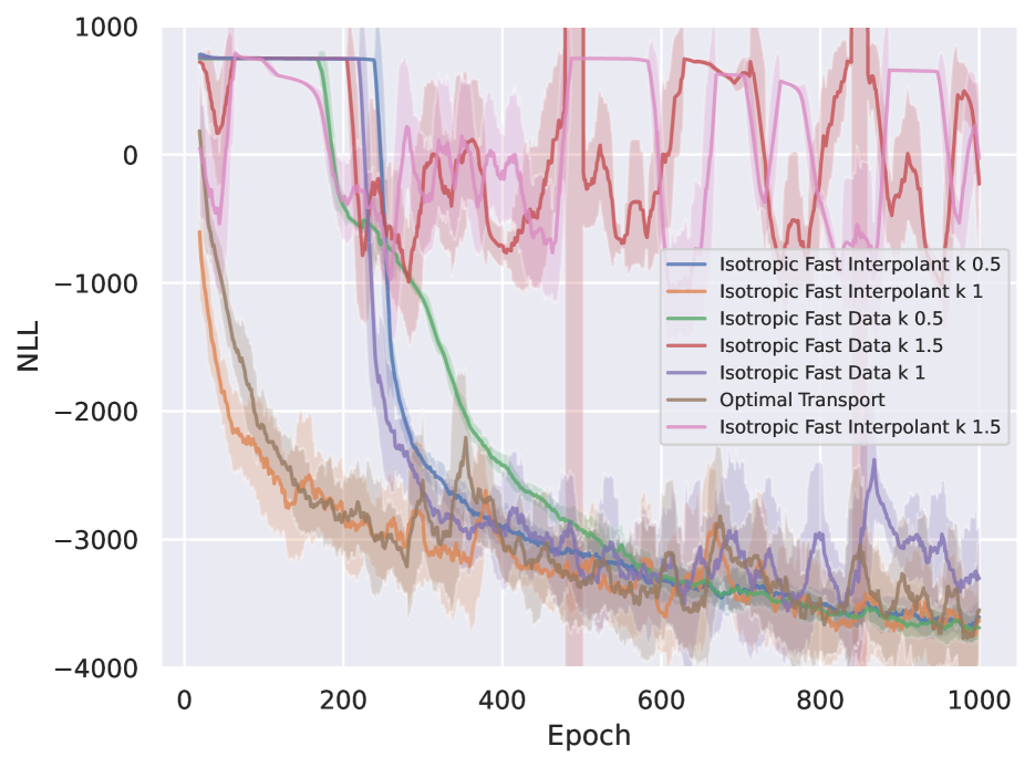
(a)

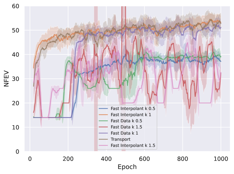
(b)

Figure 3: MNIST: The negative log-likelihood of the test set during training (a) and the number of function evaluations to compute it (b).

Table 1: MNIST Minimum negative Log-Likelihood (NLL) and Number of Function Evaluations (NFE) over the MNIST test set, where $\kappa$ is the interpolation parameter from Eq. 20.

Method	$\kappa$	NLL $\downarrow$	NFE $\downarrow$
Interpolant	1.0	-4349.63	56
Optimal Transport	–	-4294.33	56
Data	1.0	-4162.17	56
Data	0.5	-3906.55	44
Interpolant	0.5	-3863.43	38
Data	1.5	-1862.86	254
Interpolant	1.5	-1655.30	50

We devised the following conditional flow methods for MNIST

1. Data: Eq. 22 with $\boldsymbol{A}=\alpha\boldsymbol{I}$ such that $\alpha=-\ln(\epsilon/\lVert\boldsymbol{y}_{1}\rVert)$, so that $\boldsymbol{y}$ is within $\epsilon$-distance from $\boldsymbol{y}_{1}$ at $t=1$.

2. Interpolant: Eq. 22 with $\boldsymbol{A}=\alpha\boldsymbol{I}$ such that $\alpha=-\ln(\epsilon)/\kappa$, so that $z$ is within $\epsilon$-distance from $1$ at $t=1$.

For both methods we choose $\kappa\in\{0.5,1.0,1.5\}$. Intuitively, $\kappa=0.5$ would make the interpolation in Eq. 22 spend more time at the target distribution, with $z$ converging to $1$ later than $\boldsymbol{y}$ converges to $\boldsymbol{y}_{1}$. While $\kappa=1.5$ would make the interpolation spend more time at the initial distribution, with $\boldsymbol{y}$ converging to $\boldsymbol{y}_{1}$ later than $z$ converges to $1$. Additionally, we choose $\boldsymbol{B}=\beta\boldsymbol{I}$ such that the final covariance is $\boldsymbol{\Sigma}(1)=(\mathtt{1e-5})^{2}\boldsymbol{I}$. For both methods, we use the standard UNet architecture with skip connections [Ronneberger et al., 2015]. We present results for the finite training scheme (see Section 4.2), where we train to match $\boldsymbol{v}(\boldsymbol{y},z\mid\boldsymbol{y}_{1})=[\boldsymbol{v}_{y}(\boldsymbol{y},z\mid\boldsymbol{y}_{1})/v_{z}(\boldsymbol{y},z\mid\boldsymbol{y}_{1}),1]$. We use a training batch size of $500$ and train over $50000$ images. In Fig. 3, we plot the NLL and number of function evaluations over a test set of $100$ images, the results are reported in Table 1; we chose this number because it was manageable for repeated NLL calculations over epochs. With $\kappa=1$, the interpolant dynamics vary linearly with the data dynamics, resulting in simpler vector field. With $\kappa<0$, flows still converge in terms of NLL, however, the resulting vector field may be more difficult to learn. With $\kappa>1$, the flows struggle to converge at all. With the priority being data, the flows have more variability, due to the dependence of the eigenvalue of $\boldsymbol{A}$ on $\boldsymbol{y}_{1}$. With the priority being interpolant, the eigenvalue of $\boldsymbol{A}$ is constant and flows converge better.

4.4.2 Lennard-Jones 13

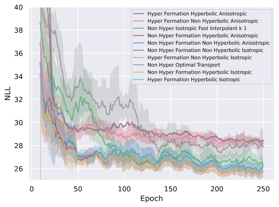
(a)

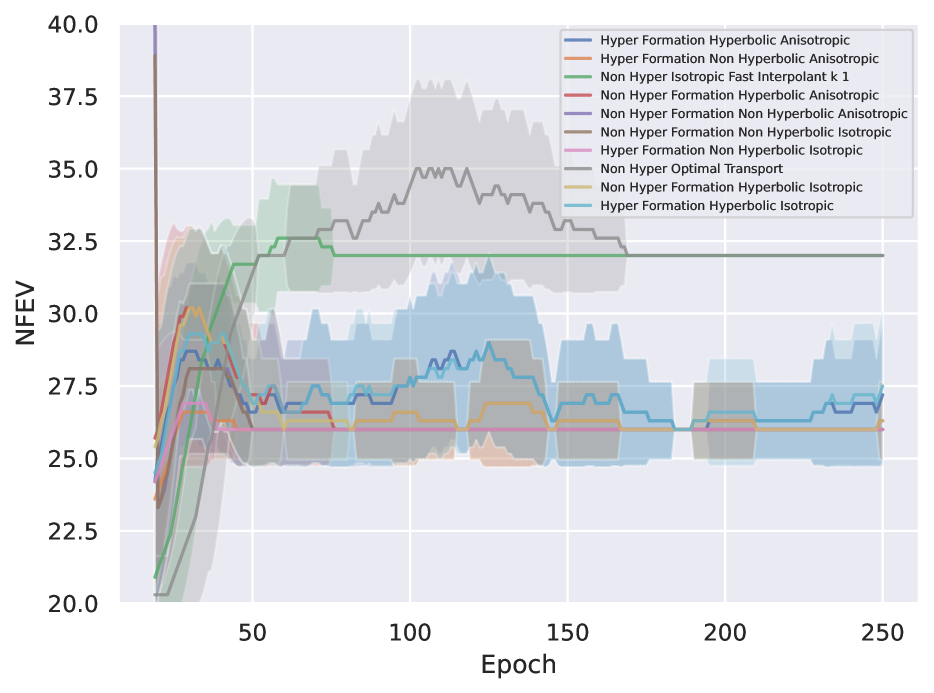
(b)

Figure 4: LJ13: The negative log-likelihood of the test set during training (a) and the number of function evaluations to compute it (b).

Table 2: LJ13: Minimum negative Log-Likelihood (NLL) and number of function evaluations (NFE) over the LJ13 test set. “Int.” refers to “Interpolant” with $\kappa=1$ from Table 1. “Form.” refers to “formation” and “OT” refers to “Optimal Transport”.

Meth.	Proj.	Hyp.	Iso.	NLL $\downarrow$	NFE $\downarrow$
Form.	✗	✓	✗	24.855	26
Form.	✗	✓	✓	24.859	26
Form.	✓	✓	✗	24.915	26
Int.	–	–	–	24.936	32
Form.	✓	✓	✓	24.937	26
OT	–	–	–	25.735	32
Form.	✓	✗	✓	26.971	26
Form.	✓	✗	✗	26.982	26
Form.	✗	✗	✓	27.095	26
Form.	✗	✗	✗	27.134	26

The Lennard-Jones 13 (LJ13) dataset consists of equilibrium configurations of $13$ three-dimensional particles of the same type, both attracted and repelled to eachother through the Lennard-Jones potential energy function [Wales and Doye, 1997]. The dataset was obtained via the link provided in [Klein et al., 2023]. For this dataset, we devised conditional flows based on the formation energy function in Eq. 25, where we consider all combinations of Projection and Hyperbolize from Section 4.3. We also consider two version of this flow with different values for $\boldsymbol{B}$ such that the flow in the hyperbolic subspace either converges to an isotropic Gaussian with variance $(\mathtt{1e-5})^{2}$ or an anisotropic Gaussian with max variance equal to $(\mathtt{1e-5})^{2}$, denoted by Isotropic in Table 2. For all the flows, we enforce a condition number of $c=2$ for the Hessian $\boldsymbol{A}$ as discussed in Section 4.3.

For all of these conditional flows, we model the marginal flow with an equivariant graph neural network [Satorras et al., 2021] with one main layer, with each MLP component having $4$ layers with $150$ features, all with softplus activation functions. We train with a batch size of $1000$ over $100000$ training samples, and report the NLL and number of function evaluations over a test set of $100$ samples in Fig. 4 and Table 2; we chose this number because it was manageable for repeated NLL calculations over epochs. We see that the NLLs during training tend to converge much faster for the flows that incorporate the Hessian information. Table 2 suggest that the “hyperbolization” discussed in Section 4.3 is helpful to improve performance. The projection of the flow matching loss into the hyperbolic subspace of the Hessian does not seem to be necessary. As the architecture used to learn the marginal vector field is already $\mathrm{SE}(3)$-equivariant, perhaps it already learns to ignore components in the nullspace of the Hessian.

Limitations

The primary limitation of the Hessian-based approach presented in this paper is that the Hessian requires $\mathcal{O}(n^{2})$ computation, and its eigen decomposition requires $\mathcal{O}(n^{3})$. As the “hyperbolization” approach seems to suffice (see Table 2), we could instead consider transforming the Hessian matrix $\boldsymbol{A}+\epsilon\boldsymbol{I}$ so that its nullspace becomes trivial, and we could then compute $\boldsymbol{A}(\boldsymbol{y}-\boldsymbol{y}_{1})$ for some $\epsilon\in\mathbb{R}_{>0}$ via a Hessian-vector product. This will be left to future work.

5 Conclusion

In this paper, we investigated the utility of using conditional flows in the flow matching framework to incorporate characteristics of the energy landscape of a Boltzman-like distribution. To do this, we showed that a linear time-invariant stochastic differential equation, based on the Hessian of an energy function, could be transformed such that it has a consistent sampling and integration time window for likelihood computation. In the process, we made several connections between flow matching, stochastic stability, topological conjugacy, group invariance, and robotic formation control. Our results show, that it is both possible incoroporate energy landscape information into flow matching and likely helpful for more complex datasets.

References

- Abramson et al. [2024] J. Abramson, J. Adler, J. Dunger, R. Evans, T. Green, A. Pritzel, O. Ronneberger, L. Willmore, A. J. Ballard, J. Bambrick, et al. Accurate structure prediction of biomolecular interactions with alphafold 3. Nature, pages 1–3, 2024.
- Blattmann et al. [2023] A. Blattmann, R. Rombach, H. Ling, T. Dockhorn, S. W. Kim, S. Fidler, and K. Kreis. Align your latents: High-resolution video synthesis with latent diffusion models. 2023 IEEE/CVF Conference on Computer Vision and Pattern Recognition (CVPR), pages 22563–22575, 2023.
- Bortoli et al. [2022] V. D. Bortoli, E. Mathieu, M. J. Hutchinson, J. Thornton, Y. W. Teh, and A. Doucet. Riemannian score-based generative modelling. In Neural Information Processing Systems, 2022.
- Bose et al. [2023] A. J. Bose, T. Akhound-Sadegh, K. Fatras, G. Huguet, J. Rector-Brooks, C.-H. Liu, A. C. Nica, M. Korablyov, M. Bronstein, and A. Tong. Se(3)-stochastic flow matching for protein backbone generation. ArXiv, abs/2310.02391, 2023.
- Bradbury et al. [2018] J. Bradbury, R. Frostig, P. Hawkins, M. J. Johnson, C. Leary, D. Maclaurin, G. Necula, A. Paszke, J. VanderPlas, S. Wanderman-Milne, and Q. Zhang. JAX: composable transformations of Python+NumPy programs, 2018. URL http://github.com/jax-ml/jax.
- Carr [1981] J. Carr. Applications of centre manifold theory, volume 35 of. Applied Mathematical Sciences, 1981.
- Chen and Lipman [2023] R. T. Q. Chen and Y. Lipman. Riemannian flow matching on general geometries. ArXiv, abs/2302.03660, 2023.
- Chen et al. [2018] T. Q. Chen, Y. Rubanova, J. Bettencourt, and D. K. Duvenaud. Neural ordinary differential equations. In Neural Information Processing Systems, 2018.
- Chi et al. [2024] C. Chi, Z. Xu, S. Feng, E. Cousineau, Y. Du, B. Burchfiel, R. Tedrake, and S. Song. Diffusion policy: Visuomotor policy learning via action diffusion. The International Journal of Robotics Research, 2024.
- Corso et al. [2023] G. Corso, B. Jing, R. Barzilay, T. Jaakkola, et al. Diffdock: Diffusion steps, twists, and turns for molecular docking. In International Conference on Learning Representations (ICLR 2023), 2023.
- Dehmamy et al. [2024] N. Dehmamy, C. Both, J. Mohapatra, S. Das, and T. Jaakkola. Hessian reparametrization for coarse-grained energy minimization. In ICLR 2024 Workshop on AI4DifferentialEquations In Science, 2024.
- Dhariwal and Nichol [2021] P. Dhariwal and A. Nichol. Diffusion models beat gans on image synthesis. Advances in neural information processing systems, 34:8780–8794, 2021.
- Dockhorn et al. [2021] T. Dockhorn, A. Vahdat, and K. Kreis. Score-based generative modeling with critically-damped langevin diffusion. In International Conference on Learning Representations, 2021.
- Duan et al. [2003] Y. Duan, C. Wu, S. Chowdhury, M. C. Lee, G. Xiong, W. Zhang, R. Yang, P. Cieplak, R. Luo, T. Lee, et al. A point-charge force field for molecular mechanics simulations of proteins based on condensed-phase quantum mechanical calculations. Journal of computational chemistry, 24(16):1999–2012, 2003.
- Esser et al. [2023] P. Esser, J. Chiu, P. Atighehchian, J. Granskog, and A. Germanidis. Structure and content-guided video synthesis with diffusion models. 2023 IEEE/CVF International Conference on Computer Vision (ICCV), pages 7312–7322, 2023.
- Feng et al. [2023] R. Feng, Q. Zhu, H. Tran, B. Chen, A. Toland, R. Ramprasad, and C. Zhang. May the force be with you: Unified force-centric pre-training for 3d molecular conformations. In Thirty-seventh Conference on Neural Information Processing Systems, 2023.
- Ho et al. [2022] J. Ho, T. Salimans, A. Gritsenko, W. Chan, M. Norouzi, and D. J. Fleet. Video diffusion models. ArXiv, abs/2204.03458, 2022.
- Hyvärinen [2005] A. Hyvärinen. Estimation of non-normalized statistical models by score matching. J. Mach. Learn. Res., 6:695–709, 2005.
- Jiang et al. [2021] H. Jiang, S. Liu, J. Wang, and X. Wang. Hand-object contact consistency reasoning for human grasps generation. In Proceedings of the IEEE/CVF international conference on computer vision, pages 11107–11116, 2021.
- Kågström [1977] B. Kågström. Bounds and perturbation bounds for the matrix exponential. BIT Numerical Mathematics, 17:39–57, 1977.
- Ketata et al. [2023] M. A. Ketata, C. Laue, R. A. Mammadov, H. Stärk, M. Wu, G. Corso, C. Marquet, R. Barzilay, and T. Jaakkola. Diffdock-pp: Rigid protein-protein docking with diffusion models. ArXiv, abs/2304.03889, 2023.
- Khalil [2002] H. K. Khalil. Nonlinear Systems. 2002.
- Klein et al. [2023] L. Klein, A. Krämer, and F. Noe. Equivariant flow matching. In Thirty-seventh Conference on Neural Information Processing Systems, 2023.
- Kœnig [1997] M. Kœnig. Linearization of vector fields on the orbit space of the action of a compact lie group. In Mathematical Proceedings of the Cambridge Philosophical Society, volume 121, pages 401–424. Cambridge University Press, 1997.
- Köhler et al. [2020] J. Köhler, L. Klein, and F. Noé. Equivariant flows: exact likelihood generative learning for symmetric densities. In International conference on machine learning, pages 5361–5370. PMLR, 2020.
- La Salle [1966] J. P. La Salle. An invariance principle in the theory of stability. Technical report, 1966.
- Le et al. [2023] M. Le, A. Vyas, B. Shi, B. Karrer, L. Sari, R. Moritz, M. Williamson, V. Manohar, Y. Adi, J. Mahadeokar, et al. Voicebox: Text-guided multilingual universal speech generation at scale. In Thirty-seventh Conference on Neural Information Processing Systems, 2023.
- Lee and Lee [2024] D. Lee and K. Lee. Multidimensional interpolants. arXiv preprint arXiv:2404.14161, 2024.
- Lindquist and Picci [1979] A. Lindquist and G. Picci. On the stochastic realization problem. Siam Journal on Control and Optimization, 17:365–389, 1979.
- Lipman et al. [2022] Y. Lipman, R. T. Q. Chen, H. Ben-Hamu, M. Nickel, and M. Le. Flow matching for generative modeling. ArXiv, abs/2210.02747, 2022.
- Liu et al. [2023] G.-H. Liu, A. Vahdat, D.-A. Huang, E. A. Theodorou, W. Nie, and A. Anandkumar. I2sb: Image-to-image schrödinger bridge. In International Conference on Machine Learning, 2023.
- Luo et al. [2021] S. Luo, C. Shi, M. Xu, and J. Tang. Predicting molecular conformation via dynamic graph score matching. In Neural Information Processing Systems, 2021.
- Mao [1999] X. Mao. Stochastic versions of the lasalle theorem. Journal of differential equations, 153(1):175–195, 1999.
- Maoutsa et al. [2020] D. Maoutsa, S. Reich, and M. Opper. Interacting particle solutions of fokker–planck equations through gradient–log–density estimation. Entropy, 22, 2020.
- Meiss [2007] J. D. Meiss. Differential dynamical systems. SIAM, 2007.
- Moler and Van Loan [1978] C. Moler and C. Van Loan. Nineteen dubious ways to compute the exponential of a matrix. SIAM review, 20(4):801–836, 1978.
- Pooladian et al. [2023] A.-A. Pooladian, H. Ben-Hamu, C. Domingo-Enrich, B. Amos, Y. Lipman, and R. T. Q. Chen. Multisample flow matching: Straightening flows with minibatch couplings. In International Conference on Machine Learning, 2023.
- Rombach et al. [2021] R. Rombach, A. Blattmann, D. Lorenz, P. Esser, and B. Ommer. High-resolution image synthesis with latent diffusion models. 2022 IEEE/CVF Conference on Computer Vision and Pattern Recognition (CVPR), pages 10674–10685, 2021.
- Ronneberger et al. [2015] O. Ronneberger, P. Fischer, and T. Brox. U-net: Convolutional networks for biomedical image segmentation. In Medical image computing and computer-assisted intervention–MICCAI 2015: 18th international conference, Munich, Germany, October 5-9, 2015, proceedings, part III 18, pages 234–241. Springer, 2015.
- Särkkä and Solin [2019] S. Särkkä and A. Solin. Applied stochastic differential equations. 2019.
- Satorras et al. [2021] V. G. Satorras, E. Hoogeboom, and M. Welling. E (n) equivariant graph neural networks. In International conference on machine learning, pages 9323–9332. PMLR, 2021.
- Shaul et al. [2023] N. Shaul, R. T. Chen, M. Nickel, M. Le, and Y. Lipman. On kinetic optimal probability paths for generative models. In International Conference on Machine Learning, pages 30883–30907. PMLR, 2023.
- Shi et al. [2021] C. Shi, S. Luo, M. Xu, and J. Tang. Learning gradient fields for molecular conformation generation. In International Conference on Machine Learning, 2021.
- Singhal et al. [2024] R. Singhal, M. Goldstein, and R. Ranganath. What’s the score? automated denoising score matching for nonlinear diffusions. arXiv preprint arXiv:2407.07998, 2024.
- Song and Ermon [2019] Y. Song and S. Ermon. Generative modeling by estimating gradients of the data distribution. In Neural Information Processing Systems, 2019.
- Song et al. [2020] Y. Song, J. Sohl-Dickstein, D. P. Kingma, A. Kumar, S. Ermon, and B. Poole. Score-based generative modeling through stochastic differential equations. In International Conference on Learning Representations, 2020.
- Sun et al. [2017] Z. Sun, B. D. Anderson, M. Deghat, and H.-S. Ahn. Rigid formation control of double-integrator systems. International Journal of Control, 90(7):1403–1419, 2017.
- Tong et al. [2023] A. Tong, N. Malkin, K. Fatras, L. Atanackovic, Y. Zhang, G. Huguet, G. Wolf, and Y. Bengio. Simulation-free schrödinger bridges via score and flow matching. In ICML Workshop on New Frontiers in Learning, Control, and Dynamical Systems, 2023.
- Vahdat et al. [2021] A. Vahdat, K. Kreis, and J. Kautz. Score-based generative modeling in latent space. In Neural Information Processing Systems, 2021.
- Vincent [2011] P. Vincent. A connection between score matching and denoising autoencoders. Neural Computation, 23:1661–1674, 2011.
- Virtanen et al. [2020] P. Virtanen, R. Gommers, T. E. Oliphant, M. Haberland, T. Reddy, D. Cournapeau, E. Burovski, P. Peterson, W. Weckesser, J. Bright, S. J. van der Walt, M. Brett, J. Wilson, K. J. Millman, N. Mayorov, A. R. J. Nelson, E. Jones, R. Kern, E. Larson, C. J. Carey, İ. Polat, Y. Feng, E. W. Moore, J. VanderPlas, D. Laxalde, J. Perktold, R. Cimrman, I. Henriksen, E. A. Quintero, C. R. Harris, A. M. Archibald, A. H. Ribeiro, F. Pedregosa, P. van Mulbregt, and SciPy 1.0 Contributors. SciPy 1.0: Fundamental Algorithms for Scientific Computing in Python. Nature Methods, 17:261–272, 2020. doi: 10.1038/s41592-019-0686-2.
- Wales and Doye [1997] D. J. Wales and J. P. Doye. Global optimization by basin-hopping and the lowest energy structures of lennard-jones clusters containing up to 110 atoms. The Journal of Physical Chemistry A, 101(28):5111–5116, 1997.
- Wu et al. [2022] L. Wu, C. Gong, X. Liu, M. Ye, and Q. Liu. Diffusion-based molecule generation with informative prior bridges. Advances in Neural Information Processing Systems, 35:36533–36545, 2022.
- Yim et al. [2023a] J. Yim, A. Campbell, A. Y. K. Foong, M. Gastegger, J. Jiménez-Luna, S. Lewis, V. G. Satorras, B. S. Veeling, R. Barzilay, T. Jaakkola, and F. Noé. Fast protein backbone generation with se(3) flow matching. 2023a.
- Yim et al. [2023b] J. Yim, B. L. Trippe, V. D. Bortoli, E. Mathieu, A. Doucet, R. Barzilay, and T. Jaakkola. Se(3) diffusion model with application to protein backbone generation. ArXiv, abs/2302.02277, 2023b.
- Yu et al. [2024] X. Yu, X. Gu, H. Liu, and J. Sun. Constructing non-isotropic gaussian diffusion model using isotropic gaussian diffusion model for image editing. Advances in Neural Information Processing Systems, 36, 2024.
- Zaidi et al. [2022] S. Zaidi, M. Schaarschmidt, J. Martens, H. Kim, Y. W. Teh, A. Sanchez-Gonzalez, P. Battaglia, R. Pascanu, and J. Godwin. Pre-training via denoising for molecular property prediction. In NeurIPS 2022 AI for Science: Progress and Promises, 2022.