Evolutionary Retrofitting

Abstract.

AfterLearnER (After Learning Evolutionary Retrofitting) consists in applying non-differentiable optimization, including evolutionary methods, to refine fully-trained machine learning models by optimizing a set of carefully chosen parameters or hyperparameters of the model, with respect to some actual, exact, and hence possibly non-differentiable error signal, performed on a subset of the standard validation set. The efficiency of AfterLearnER is demonstrated by tackling non-differentiable signals such as threshold-based criteria in depth sensing, the word error rate in speech re-synthesis, image quality in 3D generative adversarial networks (GANs), image generation via Latent Diffusion Models (LDM), the number of kills per life at Doom, computational accuracy or BLEU in code translation, and human appreciations in image synthesis. In some cases, this retrofitting is performed dynamically at inference time by taking into account user inputs. The advantages of AfterLearnER are its versatility (no gradient is needed), the possibility to use non-differentiable feedback including human evaluations, the limited overfitting, supported by a theoretical study and its anytime behavior. Last but not least, AfterLearnER requires only a minimal amount of feedback, i.e., a few dozens to a few hundreds of scalars, rather than the tens of thousands needed in most related published works. Compared to fine-tuning (typically using the same loss, and gradient-based optimization on a smaller but still big dataset at a fine grain), AfterLearnER uses a minimum amount of data on the real objective function without requiring differentiability.

1. Introduction

Retrofitting is the addition of new technology or features to older systems (Douglas, 2006; Dawson, 2007; Dixon and Eames, 2013). Retrofitting is routinely used in industry, e.g., in the building sector to adapt old buildings to new needs or new regulations. When it comes to machine learning models, the term is mainly used in natural language processing (NLP) since the seminal work of Faruqui et al. (2015a), who modify the word vector representation to take into account some semantic knowledge. This is done in a post hoc way, i.e., without retraining the whole network.

Other examples of such retrofitting (though not using that term) are used for transfer learning, when only some of the last layers of a deep neural network that had been trained for a given task are fine-tuned to another one (Oquab et al., 2023). However, even though not involving the whole set of parameters (i.e., weights), such re-trainings use gradient descent and hence only work on differentiable losses.

More generally, though differentiable machine learning (ML) has achieved significant successes, optimizing the hyperparameters of an ML pipeline (from algorithm selection to algorithm configuration) is particularly challenging, because the evaluation of a set of hyperparameters requires running a complete training cycle, or simply because the actual objective might not be differentiable.

On the opposite, gradient-free (aka black-box) optimization offers two main advantages: it does not require the computation of the gradient, thus decreasing the computational cost; and it can handle non-differentiable cost function that are out-of-reach of gradient-based methods. And there are many situations where the actual goal of the ML model is better expressed as a non-differentiable metric, and the differentiable cost used for training with stochastic gradient descent (SGD) approaches is only a proxy of such actual goal. Examples of such situation will be given in Section 5, like e.g., the number of kills in Doom video game (Section 5.3).

However, black-box optimizers generally do not scale well, and cannot be used to optimize the large set of parameters (weights) of current deep models – one significant exception being OpenAI Evolution Strategies (Salimans et al., 2017), in which Evolution Strategies are used to optimize thousands of weights of a deep neural network, as an alternative to standard deep reinforcement learning based on policy gradient approaches.

With this in mind, this work proposes AfterLearnER, for After Learning Evolutionary Retrofitting, a method that optimizes a small set of parameters or hyperparameters in a fully trained model. AfterLearnER works with any machine learning algorithm and can use a different loss function than the one used during initial training. Notably, it can handle non-differentiable loss functions, allowing for better alignment with the actual goals of the learning task without needing to run any gradient back-propagation cycle.

The overall view of AfterLearER is given in Figure 1. It can operate before test/inference time (bottom left), or at test/inference time (bottom right). In both modes, the user should proceed as follows:

• Select a small subset of the hyperparameters and/or the parameters of the model to be fine-tuned. This set of variables will be called in the following the $\aleph$-parameters. Several examples of such $\aleph$-parameters are given in the experimental Section 5, detailed in Table 2.

• Choose a focused, reliable, possibly non-differentiable, feedback signal (e.g., human feedback) as the objective of the retrofitting. In particular, it can (and will) be different from the loss used for training the model, that is required to be differentiable. Again, in order to avoid confusion with the training loss, it will be called in the following the $\aleph$-loss.

• Find approximately optimal values of the $\aleph$-parameters using a black-box optimization algorithm to minimize the $\aleph$-loss, using only the results of a few inferences on a subset of the validation set, in particular without ever retraining the whole model.

As emphasized in Figure 1, there are two modes in AfterLearnER: In both modes, AfterLearnER operates after the classical backprop training. In offline mode (Figure 1-bottom left, examples in Sections 5.1, 5.2, 3, 5.3 and 5.4), AfterLearnER optimizes the $\aleph$-parameters w.r.t. the $\aleph$-loss once and for all, using some low-volume coarse grain validation data. In particular, it only needs a few inferences of the trained model (and in particular no gradient backpropagation).

In online mode (Figure 1-bottom right and  Sections 5.5, 5.6 and 5.7), AfterLearnER optimizes the model answer to each test cast during inference, and the $\aleph$-parameters can typically contain some latent variables, input to the model. This amounts to online retraining, based on some small aggregated feedback (SAAF as defined in Section 4.4).

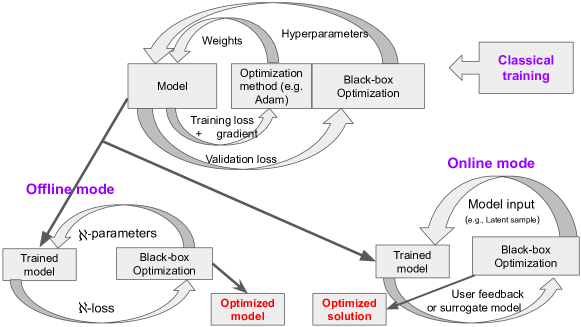
Figure 1. AfterLearnER vs Classical ML. Top: Standard gradient-based training (e.g., backpropagation) and hyperparameter tuning (the outer loop). Bottom: The two modes of AfterLearnER. Left: In the offline mode, retrofitting of some parameters (termed $\aleph$-parameters, see text) of the trained model, once and for all before test time, as in Sections 5.1, 5.2, 5.3 and 5.4, and the output of AfterLearnER is an optimized model. Right: In the online mode, the $\aleph$-parameters can also include some model input in the latent space, the objective can then be dynamic (the loss, the user feedback, or a surrogate model), as in Sections 5.5, 5.6 and 5.7. The output of AfterLearneER is then an improved output for the given input.

AfterLearnER clearly relates to hyperparameter optimization (HPO) (Feurer and Hutter, 2019), transfer learning (Zhuang et al., 2021), and fine tuning (Lialin et al., 2023) approaches. Also, because AfterLearnER is performed after standard training, it semantically relates to a number of test-time adaptation (TTA) approaches (Niu et al., 2022; Chen et al., 2022). The main difference with such previous works is that AfterLearnER can handle non-differentiable losses, possibly closer to the actual objective of the learning task. AfterLearnER can also be used to handle distributional data shift (like TTA approaches), or to adapt the pre-trained mode to new tasks, as in transfer learning (Oquab et al., 2023), though it is initially conceived to improve the pre-trained model for the same task, the $\aleph$-loss providing a different point of view on the task at hand. These issues will be discussed in more detail in Section 2.1 below, and illustrated by the experiments in Section 5.

The paper is organized as follows. Section 2 introduces the context of this work: Section 2.1 surveys related works, Section 2.2 discusses non-differentiable losses, and Section 2.3 introduces the black-box optimization algorithms used in AfterLearnER. Section 3 presents AfterLearnER in detail, following some kind of “user guide” format. Section 4 discusses a priori the advantages of the proposed methodology. Section 5 presents the experimental results obtained across various applications, by AfterLearnER in offline mode for Depth sensing (Section 5.1), speech re-synthesis (Section 5.2), reinforcement learning for Doom video-game (Section 5.3), and code translation (Section 5.4); And by AfterLearnER in online mode for 3D-GANs (Section 5.5), and text-to-image (Sections 5.6 and 5.7). Finally, Section 6 globally discusses the results, and Section 7 concludes the paper.

2. Background

2.1. Related work

AfterLearnER is related to a number of previous works, with some significant differences that are summarized in Table 1 along different axes, and will be discussed in turn in this Section. We are aware that many other works could have been cited here. We nevertheless did our best to cover the most prominent lines of related work, even if not citing all relevant papers in each subsection below.

Table 1. Comparison between different works related to AfterLearnER. The columns from left to right are: Whether their target task is the same as the one used during pre-training; Whether any additional knowledge is needed for the optimization; What proportion of the model parameters are modified; Whether some gradient is needed or not; The number of full backprop optimization that are performed (if any) after the pre-training; The corresponding typical references (there are dozens of other works, and we cannot pretend to be exhaustive).

. Framework Final Additional Reoptimized Gradient needed Additional References task knowledge parameters Full Backprop Hyperparameter tuning Same – Small part No (outer loop) Many ¡1¿ Fine tuning Different Smaller dataset Depends Yes A few ¡2¿ Transfer learning Different Distinct dataset Entire net Yes A few ¡3¿ Test-Time Training Same – Large part Yes A few ¡4¿ Test-Time Adaptation Same – Small part Yes None ¡5¿ Retrofitting Same High-level info Small part Depends None ¡6¿ Small part No AfterLearnER Same Coarse grain info or latent vars (possibly interactive) None

¡1¿ Feurer and Hutter (2019) ¡2¿ Lialin et al. (2023) ¡3¿ Zhuang et al. (2021) ¡4¿ Sun et al. (2020) ¡5¿ Wang et al. (2021) ¡6¿ Faruqui et al. (2015b)

2.1.1. Hyperparameter Tuning

Hyper-parameter optimization (HPO) has become routine in the ML world in general (see e.g., Feurer and Hutter (2019) for a survey), and in deep learning in particular. The $\aleph$-parameters are the usual hyperparameters of the training pipeline, and can include architecture parameters (HPO is then called neural architecture search (NAS)). The optimization is then a two-tiered process, as shown in Figure 1-top, in which the inner loop is a full backprop optimization, and the outer loop is a black-box optimization (e.g., Bayesian (Kandasamy et al., 2018) or Evolutionary (Assunção et al., 2019) optimization. But the process is extremely costly because the loss is then the performance of the fully re-trained network. As such, we will not consider it as an alternative to AfterLearnER.

2.1.2. Fine-tuning and transfer learning

Fine tuning has become now a routine process in deep learning (Lialin et al., 2023). It is used for instance to specialize general purpose LLMs for downstream tasks (Ouyang et al., 2022), including supervised learning and Reinforcement Learning from Human Feedback (see Section 2.1.5 below). Still in the context of LLMs, it can be used to “improve” the outcomes of the model following the programmer’s preferences (Rozado, 2023). In such situations, the whole model is fine-tuned using standard gradient-based optimization of the training loss itself, and even though only a fraction of the iterations is needed, this still has a significant cost.

Another use of fine tuning relates to Transfer Learning (Zhuang et al., 2021): A model that has been trained for a specific task can be fine-tuned to perform a different but similar task, freezing most of the model, optimizing only a fraction of it (e.g., one or a few last layers). Under some mild hypotheses, it has been demonstrated (Lu et al., 2022; Giannou et al., 2023) and later proved (Burkholz, 2024) that normalization layers are indeed good candidates for such fine-tuning. Still, the number of $\aleph$-parameters can be rather high (e.g., more than 100,000 in (Lu et al., 2022)). Furthermore, here again, a few iterations of full backprop optimization is needed, meaning that the loss should be differentiable, and the optimization might be costly (in compute and/or memory). The latter approach is sometimes referred to as Feature Extraction: the frozen first layers de facto become feature constructors.

As its name says, however, the goal of transfer learning is to handle tasks that are not the ones for which the model was pre-trained, or modify the behavior of the model, whereas the main goal of AfterLearnER is to improve the outputs of the model on the task for which it was initially trained, possibly using a non-differentiable $\aleph$-loss that better describes the desired behavior of the model. Also, the $\aleph$-parameters that are tuned AfterLearnER are generally much smaller than those of the above works, even when most parameters are frozen.

2.1.3. Test-Time Training / Adaptation

Whereas fine tuning and transfer learning generally pertain to supervised learning, in that they require labeled examples of the possibly new task, there are many real world situations where such labels are not available. A large body of work has been devoted to such contexts, in particular to handle the case of distribution shift between training and testing times, pertaining to unsupervised domain adaptation. A survey and discussion of several of such approaches is given in (Niu et al., 2022).

A first line of research assigns some labels to the unlabeled test data, and performs some test time training. Such labels can be self-supervision labels, e.g., the number of $90\mathrm{°}$ rotations in images (Sun et al., 2020) and the upper layers of the pre-trained model are gradually modified by standard backprop; or one can use some pseudo-labels obtained from a copy of the pre-trained model that is gradually updated (Chen et al., 2022). In both cases, however, the size of the $\aleph$-parameters that are modified is rather big (a large fraction of the original model), and the $\aleph$-loss must be some usual supervised training loss, hence differentiable.

On the other hand, test-time adaptation (TTA), as proposed by Wang et al. (2021), and further refined by, e.g., Niu et al. (2022, 2023), performs some generic entropy minimization, and only optimizes some affine transformation parameters of the normalization layers of the original deep network, in order to fully preserve the pre-trained model. TTA $\aleph$-parameters are hence very small, a feature shared with AfterLearnER. However, the entropy minimization is gradient-based, and the $\aleph$-loss is limited to the chosen entropy — or possibly another differentiable loss (Goyal et al., 2022).

The main advantage of AfterLearnER compared to test-time adaptation remains the possible use of non-differentiable $\aleph$-loss, together with the small compute needed in most cases (see Section 5).

2.1.4. Retrofitting for NLP

Retrofitting in natural language processing enhances word vector representations by refining them with relational information from semantic lexicons. This post-processing technique adjusts pre-trained word vectors so that semantically related words are closer in the vector space.

Faruqui et al. (2015b) introduced a graph-based retrofitting method that refines word vectors by using belief propagation on a graph constructed from lexical relationships. It encourages linked words to have similar vector representation. This process retains the original distributional properties while integrating relational information. ConceptNet (Speer et al., 2017), a multilingual knowledge graph, links words and phrases through labelled edges and improves the understanding of word meanings. When combined using retrofitting with word embeddings, it forms a hybrid semantic space called ConceptNet Numberbatch (Speer et al., 2017), which provides a richer understanding of language. In summary, retrofitting for natural language processing leverages external knowledge to refine word vectors, enhancing their quality and interpretability for various natural language processing tasks. Both AfterLearnER and the above works aim to take new knowledge into account in order to improve the task the model was pre-trained on, by modifying a few of its parameters. However, AfterLearnER can modify any type of $\aleph$-parameters, and is not limited to modifying some latent representation in the model. Furthermore, AfterLearnER uses far less new knowledge than the full lexicons required by NLP retrofitting approaches (Chiu et al., 2019).

2.1.5. Reinforcement Learning from Human Feedback

A particular case of non-differentiable feedback is human feedback. Reinforcement learning from human feedback (RLHF) has recently gained importance in image generation (Lee et al., 2023b) and large language models (LLMs). However, most low-budget RLHF papers (working with dozens or hundreds of human feedback samples) are in the field of robotics (Jain et al., 2015). The trend in LLMs is more in the dozens of thousands, or even the millions (Abramson et al., 2022). However, a limited human feedback is sometimes sufficient (Kim et al., 2023) and real-time user-specific preferences can sometimes be taken into account (Videau et al., 2023). Low-budget RLHF could be based on inverse reinforcement learning (IRL) i.e., simulating human preferences from preference signals in a reward model (Adams et al., 2022). To reduce the need of abundant ground truth data, it is important to focus on small but impactful weights of the model. As already mentioned in Section 2.1.2, Lu et al. (2022); Giannou et al. (2023); Burkholz (2024) present such small impactful parts, the normalization layers, which are relatively small but intersect entirely the information flow from input to output.

2.2. Non-differentiable reward functions and feedbacks

Stochastic gradient descent and its many variants perform extremely well for many machine learning tasks, but can only handle differentiable feedbacks. Criteria like those used in depth estimation, human satisfaction (as in translation or image generation), or large-scale simulators (e.g., Doom) are beyond gradient-based approaches.

Therefore, the design of specific reward functions, typically in the realm of reward shaping (Ng et al., 1999), is critical. In particular, one must be careful with reward hacking (Skalse et al., 2023) and transferability. In (Wang et al., 2021; Niu et al., 2023; Lee et al., 2023a), differentiable criteria are designed as proxies to the actual target criteria, adding one level of approximation to the goal, and hence leading to less accurate solutions. The point of the present work is to bypass such approximation errors by directly using possibly non-differentiable criteria and arbitrary combinations thereof.

In terms of optimization algorithms, Rolinek et al. (2020) proposes a method specifically for rank-based criteria. Jiang et al. (2020); Huang et al. (2021) propose to approximate non-differentiable reward functions by differentiable scores. Hiranandani et al. (2021) focuses on criteria defined on the confusion matrix. Sun et al. (2022) focuses on a random subspace of a huge parameter space. Susano Pinto et al. (2023) applies the Reinforce (Williams, 1992) algorithm. On the opposite, AfterLearnER is based on generic black-box optimization (Section 2.3).

2.3. Tools for black-box optimization

Black-box optimization refers to optimization methods which only need, from the objective function $f$, the value of $f\left(x\right)$ when providing $x$. In particular, no gradient is used, and no knowledge of the internal structure of $f$ is necessary. Evolutionary Algorithms (Eiben and Smith, 2015) and Iterated Local Search (Stützle and Ruiz, 2018) are examples of black-box optimization tools.

Algorithm 1 outlines the functioning of all algorithms used in this study, within a parallel computing context, utilizing the the well-known ask-and-tell interface: the algorithm $o$ is defined by its methods $initialize$, $tell$ (informs $o$ of the value of $f(x)$), $ask$ (returns next value $x$ to evaluate), and $recommend$ (returns its best guess for the optimum).

objective function $f$, number of workers $P\geq 1$, domain $D$, budget $b$

$o.initialize\left(D,b,P\right)$ $\triangleright$ Initialize $o$ given $P$, domain $D$, and budget $b$

procedure Worker-task($x$)

     Compute $f\left(x\right)$

      $o.tell\left(x,f\left(x\right)\right)$ $\triangleright$ Inform the method $o$ of the performance obtained by the $\aleph$P $x$, no gradient needed

end procedure

for $i\in\{1,\dots,b\}$ do

     Wait until there are less than $P$ computations in progress in the FIFO

     Request $x\leftarrow o.ask\left(\right)$ ($x\in D$) $\triangleright$ Choice of $\aleph$-parameters to be tested

     Put $x$ in the FIFO of workers tasks

end for

Wait until the FIFO is empty

return $o.recommend\left(\right)$ $\triangleright$ Final returned value

Algorithm 1 General organization of a parallel asynchronous black-box optimization method $o$. There is a first-in-first-out (FIFO) pool of pairs $\left(x,f\left(x\right)\right)$ to be computed by the workers. The sequential case corresponds to $P=1$.

There are many libraries for black-box optimization. AfterLearnER uses Nevergrad (Rapin and Teytaud, 2018) that implements Evolutionary Algorithms (Eiben and Smith, 2015), Mathematical Programming (Powell, 1994, 1964), or handcrafted combinations (Meunier et al., 2022b).

In terms of black-box optimization tool, AfterLearnER can run several times, using different methods, as developed in Algorithm 2. By default, it uses a single algorithm, namely an optimization wizard (Appendix B), namely NGOpt (Meunier et al., 2022a), which automatically selects a relevant algorithm based on the available computational budget, the problem dimension, and the types of variables to optimize. More precisely, the algorithms available to the wizard include DiagonalCMA (Ros and Hansen, 2008; Hansen and Ostermeier, 2003), Differential Evolution (DE) (Storn and Price, 1997), Particle Swarm Optimization (PSO) (Kennedy and Eberhart, 1995), Lengler (Doerr et al., 2019), among others. When we pick up several algorithms instead of just NGOpt, we follow the recommendations described in the Nevergrad documentation for choosing the different algorithms, as detailed later. A benchmark of the many existing black-box optimization methods is beyond the scope of this paper.

3. The AfterLearnER Algorithm and its Experimental Setting

3.1. AfterLearnER

The AfterLearnER algorithm and its default parameter settings are presented in Algorithm 2. Given an $\aleph$-loss (Section 4.3) to be minimized on some validation set $\mathcal{V}$ (running the trained model at hand on the data points in $\mathcal{V}$), AfterLearnER needs an integer $k$ (number of runs), a list of black-box optimization algorithms, and a list of possible budgets. It then loops k independent times (6 ), launching (Line 4) one randomly chosen black-box algorithm in the list (Line 2) to minimize the $\aleph$-loss on $\mathcal{V}$ for one of the available budgets (Line 3). The result of the run is stored (Line 5) and the best results of the $k$ runs is returned by AfterLearnER (Line 7).

By default, the list of black-box algorithms is made of a single algorithm, the wizard $NGOpt$ (Meunier et al., 2022a), presented in more details in Appendix B. As a wizard, it can work in all dimensions/domains/budgets. The budget and the number of runs depend on the expected computational cost and the available overall compute budget. See Table 3 for some examples of AfterLearnER settings used in this work.

1:$\aleph$-loss $l$

2:$\mathcal{V}$ validation set

3:List of black-box optimization algorithms $O$ $\triangleright$ By default $O=\{NGOpt\}$

4:List of budgets $B$ $\triangleright$ No default value

5:Number of independent runs $k$ $\triangleright$ By default 1

6:for $i\in\{1,\dots,k\}$ do

7:     Randomly draw $o_{i}\in O$ $\triangleright$ only if $\#O>1$

8:     Randomly draw $b_{i}\in B$

9:     Run $o_{i}$ to minimize $l$ on $\mathcal{V}$ with budget $b_{i}$

10:     $\aleph$-parameters $p_{i}=o.recommend()$ $\triangleright$ The result of the optimization

11:end for

12:return $\aleph$-parameters $p_{i}$ that minimizes $\aleph$-loss $l$ on $\mathcal{V}$, $i\in[1,k]$

Algorithm 2 The AfterLearnER algorithm.

3.2. The Experiments

AfterLearnER is validated in Section 5 on eight problems, whose characteristics are given in Table 2, while the corresponding AfterLearnER $\aleph$-parameters are given in Table 3. The choice of these test beds and their setups have been guided by the following principles, that can be viewed as a kind of User Guide for AfterLearnER.

1. Optimize a small but impactful part: Lu et al. (2022); Giannou et al. (2023); Burkholz (2024) have demonstrated how a small part of the parameters of an ML model can have a big impact on its performance. Typically, for a huge network or a combination of modules, one should look for a smallest set of parameters that intersects all paths from inputs to outputs. Furthermore, it is important to keep the dimension of the optimization problem small: black-box optimization algorithms do not scale up well in general — opposite to gradient-based optimization algorithms, The list of what is optimized in this paper is summarized in Table 2, middle column. Except for Doom, the number of evaluations of $\aleph$-parameters is small compared to e.g., (Zhu et al., 2023; Arakawa et al., 2018)

2. Don’t fear non-differentiable $\aleph$-losses: This is the main advantage of AfterLearnER: Lu et al. (2022); Giannou et al. (2023); Burkholz (2024) work on a small part (as we do), but with differentiable criteria. There are many methods for differentiable optimization in machine learning: gradient-free algorithms cannot outperform these methods unless the gradient is not reliable. We note that (Niu et al., 2022, 2023; Lee et al., 2023a) propose to create (possibly without any human feedback or ground truth, thanks to unsupervised entropy minimization) a differentiable criterion based on entropy. However, AfterLearnER focus is on cases in which a non-differentiable criteria is worth a direct optimization.

Table 2. Problems tackled in the present paper. The size of the $\aleph$-parameters optimized by AfterLearnER varies between 1 and 16384. All the feedbacks in this table are not differentiable. For comparison, a classical ML training with $e$ epochs on a dataset of cardinal $S$ and a gradient of size $p$ has a feedback of size $({\mathbb{R}}\cdot{\mathbb{R}}^{p})^{e\cdot S}$.

Problem	$\aleph$-parameters	Feedback volume	Type of feedback
Depth sensing (Section 5.1)	$6$ input normalization parameters	300 feedbacks by the large model (${\mathbb{R}}^{300}$)	Depth estimate by the large model
Speech resynthesis	$2$ hardcoded constants	40 automatically computed feedbacks for TextLess (${\mathbb{R}}^{40}$)	Word error rate
3D Gan	latent variable $z$ (problem dependent)	Image quality (200 user inputs, one per image, total ${\mathbb{R}}^{200}$)	Human rating
LDM + input text	latent variable $z$ ($4\cdot 64\cdot 64$)	Variable, a few clicks	Human ratings
Doom AI	Rescaling of the output layer ($35$ weights)	Kills per life in VizDoom, ${\mathbb{R}}^{60000}$	VizDoom simulation
Code Translation	Rescaling between encoder & decoder ($1024$)	BLEU + comp. accuracy on valid set (${\mathbb{R}}^{1000}$)	Automatically computed score

Table 3. AfterLearnER parametrization in our experiments. In the case of LDM, we use a Voronoi crossover described in Section 5.7.

Problem	Optimizer $O$	Budget $B$ per run
Depth sensing	$\{NGOpt\}$	$\{300\}$
Speech resynthesis	$\{NGOpt\}$	$\{2,10,20,40,80\}$
Image generation	$\{Lengler\}$	user stopping
Image generation Fairness	$\{RandomSearch\}$	$\{30\}$
Doom AI	$\{OptimDisc(1+1)\}$	$\{300,600,800,1000,1200\}$
CodeGen translation	$\{DiagonalCMA\}$	$\{1000\}$
EG3D-cats	$\{RandomSearch\}$	1000⋆
EG3D-cats with diversity	$\{NGOpt\}$	1000⋆
LDM	Ad hoc (incl. Voronoi crossover)	a few batches

3.3. Discussion

Before detailing the experimental validation, we take a look at the a priori benefits of retrofitting on the problems described in Table 2, according to the rationale developed in Section 4.

Table 2 shows in particular the different sizes of the feedback used in the following. It can always be provided by humans or computationally expensive solvers. Regarding RLHF (such as EG3D, LDM), we consider feedback limited to dozens or hundreds of scalars (far less than most works as discussed in Section 2.1.5).

For speech re-synthesis Section 5.2 and depth sensing Section 5.1, the number of runs is $k=1$ because of the computational cost (for depth and speech) or limited human attention span (for image generation).

Our approach requires less data and utilizes feedback at a more aggregated level, compared to most RLHF (Zhu et al., 2023) and Human In The Loop Reinforcement Learning (HITLRL (Arakawa et al., 2018)) approaches. Specifically, our approach needs only one objective function value per model and dataset. In contrast, classical stochastic-gradient methods require one objective function value and one gradient value per model and per data point. The process is hence compatible with evaluation by humans, who can study an entire system output, and compare on key points (see e.g., human feedback ), or with end-of-episode (delayed) evaluations by complex simulators (e.g., VizDoom (Kempka et al., 2016) for Doom, Section 5.3) or non-differentiable computational accuracy (in code translation Section 5.4).

4. Rationale for AfterLearnER

This section discusses a priori the potential benefits of using retrofitting, beyond the obvious generic advantages of any gradient-free optimization: one can work in settings in which the gradient cannot be computed or does not make any sense, e.g., discrete metrics or discrete domains.

4.1. Computational cost

Even when the gradient exists and is easy to compute, it might require a large computational cost, and re-optimizing billions of weights for each value of the hyperparameters is time-consuming. AfterLearnER has a low computational cost: no gradient needs to be computed during AfterLearnER, therefore saving the memory and computation costs of the backward pass. Table 3 attests that our budgets are small.

4.2. Branching factor analysis for a low overfitting

Whereas gradient-based optimization does not lead to any bound on the generalization error, such bounds can be obtained when using black-box optimization, as detailed below. These bounds suggest that the risk of overfitting is lower. Indeed, following (Fournier and Teytaud, 2011), consider $\delta$ the risk of an $\epsilon$-divergence between the empirical risk and the risk in generalization for a given $\aleph$-parameters, i.e., $P(|(expected\ loss)\ -\ (empirical\ loss\ on\ dataset)|>\epsilon)\leq\delta$. If we use the validation error for picking up the best $\aleph$-parameters, in a list of $N$ $\aleph$-parameters, the risk of deviation $\epsilon$ for that $\aleph$-parameters is at most $N\cdot\delta$ (Bonferroni correction (Bonferroni, 1936)) instead of $\delta$:

$$P(\exists c\mbox{ a $\aleph$-parameters{}},|(expected\ loss)_{c}\ -\ (empirical\ loss\ on\ dataset)_{c}|>\epsilon)\leq N\delta.$$

If the $N$ $\aleph$-parameters are not defined a priori but built by optimization, with $\lambda$ $\aleph$-parameters per iteration and selection of the best at each iteration, then the total risk is at most $\lambda^{n}\cdot\delta$ where $n$ is the number of iterations ($\lambda$ evaluations in each iteration) (Fournier and Teytaud, 2011). And if the total number of evaluations is $N$, then $n=N/\lambda$ and the total risk is at most $\lambda^{N/\lambda}\cdot\delta$.

Furthermore, if $k$ independent runs of AfterLearnER are run, and if the budget $N$ is divided by $k$, then the Bonferroni correction leads to a risk

$$\underbrace{k}_{\text{Bonferroni correction for $k$ runs}}\cdot\underbrace{\lambda^{(N/(\lambda\cdot k))}}_{\text{Branching factor per run}}\cdot\underbrace{\delta}_{\text{Risk for a single model}}$$

for the resulting parametrization. According to these bounds, increasing the number $k$ of independent runs, for a given total budget, decreases the risk of overfitting. Also, according to this bound, increasing the parallelism $\lambda$ decreases the risk of overfitting.

4.3. Versatility, convenience

Black-box optimization is very versatile, allowing the user to easily explore different objective functions. For Doom (Section 5.3), for fair comparisons, we report results on the same losses than the ones used by the authors of previous works (Lample and Chaplot, 2017). However, a significant benefit of AfterLearnER is its ability to adapt a model to a different loss, the $\aleph$-loss, without the need to manually craft reward shaping, or using an approximate proxy.

We note that the approach can be applied for the optimization of a complex system, including several deep learning (DL) models combined with other mathematical programming tools or signal processing methods, even if some of these blocks are non differentiable, as illustrated by the experiments presented in Section 5.

4.4. Small Aggregated Anytime Feedback

The arguments for the potential benefits of AfterLearnER can be summarized by the acronym SAAF, for Small Aggregated Anytime Feedback:

• Small: A few dozens scalars is enough, as will be demonstrated in the experiments (see Table 2).

• Aggregated: A feedback of one scalar per model is sufficient, instead of one scalar per data point or one scalar and a gradient for each mini-batch. This is visible in our applications when training once and for all a model between training and testing, in Sections 5.1, 5.2, 5.3 and 5.4.

• Anytime: AfterLearner can be stopped when desired, given the real-time user feedback (Zilberstein, 1996).

5. Experiments

This section presents different experiments demonstrating that black-box optimization can indeed take advantage of SAAF to significantly improve a pre-trained model. The computational cost is discussed in Appendix D.

The first four experiments, Depth Sensing (Section 5.1), Speech Resynthesis (Section 5.2), Doom (Section 5.3) and Code Translation (Section 5.4), pertain to the offline mode, and directly use (Algorithm 2). The last three experiments, 3D-GANs with EG3D (Section 5.5), LDM with human feedback (Section 5.6), and Interactive LDM (Section 5.7) present experiments that use AfterLearnER in online mode: AFterLearnER is then tightly embedded in the inference process.

5.1. Depth sensing

5.1.1. Context

MiDaS (Ranftl et al., 2022) is a famous deep network for monocular depth estimation from a single image. This neural network exists in three trained variants: large, hybrid and small. The large one, known for its precision (Birkl et al., 2023), is considered here as the ground truth.

As in (Ranftl et al., 2022), ImageNet images are first resized to $144\times 144$ pixels. Then AfterLearnER (Algorithm 2) uses a set $\mathcal{V}$ of 300 images randomly drawn from ImageNet validation set (of size 50,000). With $b=50$, the feedback used by AfterLearnER is made of the 50 scalars obtained in applying 50 variants of the model (corresponding to different $\aleph$-parameters iteratively provided by AfterLearnER) to the images in $\mathcal{V}$, for each of the $k$ runs. Furthermore, a set ${\mathcal{V}}^{\prime}$ of 500 images randomly drawn from ImageNet test set is used to assess AfterLearnER performance.

5.1.2. $\aleph$-parameters

AfterLearnER tunes the 6 normalization parameters (multiplication and bias for each of 3 channels) for optimizing the $\aleph$-loss on $\mathcal{V}$. We use the code available at github.com/isl-org/MiDaS.

5.1.3. $\aleph$-loss: Estimating depth

Yin et al. (2020) point out that there exist several depth estimation criteria, created for different applications: a criterion which is good for local differences (relative depth) might be plain wrong for global profiles. Therefore, a diversity of criteria has been proposed, including, among others, the absolute relative error (AbsRel), the weighted human disagreement rate  (Xian et al., 2018), the scale-invariant root-mean-square error (Li et al., 2019), or the frequency of obtaining a mismatch greater than a given threshold (Ranftl et al., 2022). These different losses are used in different areas (Paul et al., 2022; Hwang et al., 2021; Ma and Karaman, 2018).

Following (Ranftl et al., 2022), we focus here on the frequency of failing, by a factor greater than $1.25^{i}$, with $i=1,2$, or $3$ (further referred to as Threshold $i$). These criteria are not continuous, and are flat almost everywhere so that their gradient is essentially zero.

5.1.4. Results

Algorithm 2 is launched here with values $O=\{NGOpt\}$, $B=\{b\}$ (by default $50$), and for different values of $k$.

Figure 2 displays the $\aleph$-loss on the test set $\mathcal{V}^{\prime}$ versus the number of runs $k$ for a budget of 50 (other results are presented in Appendix A). These results demonstrate an enhancement in the $\aleph$-loss optimized using the validation set, consistently improving the performance of the Small baseline, and sometimes outperforming the performance of the Hybrid model, even with $k<10$. Appendix A also presents evidence of effective transferability: specifically, training on Threshold 3 (i.e. with ratio $1.25^{3}$) does not only improve outcomes in the test set for that metric, but also yields positive results for other metrics discussed in Section 5.1.3 above.

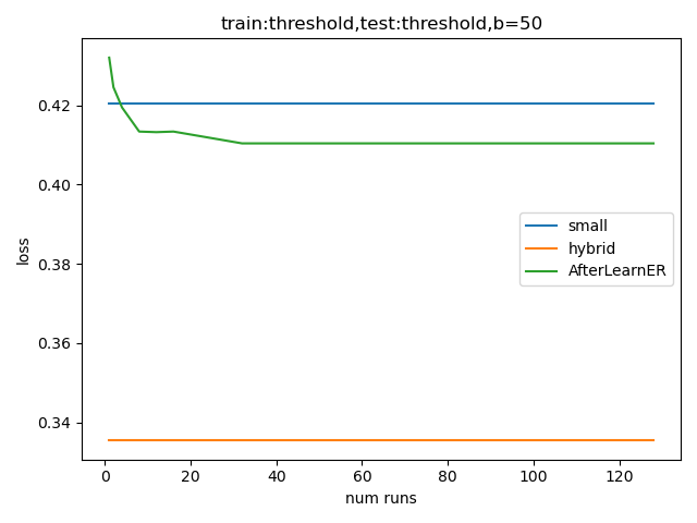
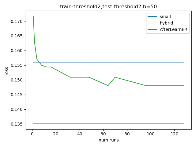
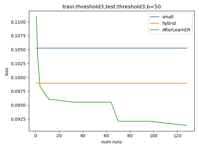
Figure 2. Losses on the test set $S^{\prime}$ of the small and hybrid models, and of AfterLearnER after optimizing criteria Thresholds 1 (left), 2 (middle) or 3 (right), with $b=50$ and for different values of $k\geq 1$.

5.1.5. Discussion

Whereas no more than 50 scalars of feedback are necessary for AfterLearnER to improve the Small model, we note that with larger budget, we sometimes outperform the intermediate (a.k.a hybrid) model with just 300 scalars (e.g., $k=6$ and $b=50$ in Figure 2). We observe that results are robust and are effectively transferred to different loss functions (Appendix A). Because $k$ runs of budget $b$ amounts to $k\cdot b$ scalars, $300$ feedbacks could eventually be asked to human raters, though in the present case we actually (for the sake of reproducibility) use the large MiDaS model as a ground truth.

5.2. Speech resynthesis: a few dozens feedbacks for improving sound quality

TextLessLib (Kharitonov et al., 2022) is a deep learning library for speech synthesis without text representations. It includes a demo of speech resynthesis (Polyak et al., 2021) from low bit rates.

5.2.1. Context

The discrete resynthesis operation can be viewed as a form of lossy compression for speech. Approaches such as (Polyak et al., 2021) directly train in the waveform using an autoencoder, with adversarial and reconstruction loss. Here, we diretly optimize the Word Error Rate (WER) (Kharitonov et al., 2022), which is not differentiable. We use data and code from (Polyak et al., 2021), splitting the training data into 75% for the $\aleph$-parameters optimization and 25% as a test set post-optimization. The results can, therefore, not be compared numerically to the results in the original work: we use an additional information. Nonetheless, the results show that a few dozen scalar feedbacks are enough for a significant improvement.

5.2.2. $\aleph$-parameters

AfterLearnER handles here two $\aleph$-parameters of the Tacotron/Vocoder model (Wang et al., 2017): the sigma in WaveGlow/inference (Prenger et al., 2019) and the denoiser strength. These two $\aleph$-parameters are hardcoded in the original code.

5.2.3. $\aleph$-loss: Word-Error-Rate

This measure evaluates how accurately the audio can be transcribed after compression, assessing how well the textless compression preserves speech-specific characteristics and clarity. We compute the WER through the wav2vec 2.0-based (Baevski et al., 2020) and Automatic Speech Recognition (ASR) system: the code compares the output with the ground-truth transcription. The WER is also used to evaluate our retrofitted model on the test set.

5.2.4. Results: robust low budget quality improvement

The results of applying different parameterizations in Algorithm 2 are presented in Table 4. One can observe that picking up the best outcome from multiple shorter runs (i.e., a large number of runs ($k$) with a small budget ($b$) per run) yields the most favorable results. In certain instances, the number of runs ($k$) is even so large, and the budget per run so limited that the approach nearly resembles a random search (e.g., a $9.9\%$ improvement observed with the best of 8 runs each having a budget of 2). These experiments demonstrate that AfterLearnER can significantly improve test results at a low cost within a few evaluations on a small validation set.

5.2.5. Discussion

Table 4 shows that in this test case with minimal sample size, the utilization of a high number of runs consistently enhances performance in generalization, aligning with the theoretical discussions presented in Section 4.2: such results experimentally demonstrate the reduction of the risk of overfitting by using a large number of runs and a small budget per run.

Table 4. Performance on the test set in textless Speech Resynthesis for different values of $k$ in Algorithm 2. The baseline WER is 7.84: for each scenario, several replicas are run: 100% of scenarios lead to an improvement on average.

Num runs $k$	Budget	WER $(\downarrow)$	Avg. improvement (%, $\uparrow$)	Std of WER
	2	7.488	4.511	0.335
	10	7.558	3.620	0.202
	40	7.736	1.361	0.235
3	80	7.542	3.828	0.298
	2	7.306	6.837	0.387
	10	7.501	4.355	0.147
	40	7.751	1.163	0.217
4	80	7.378	5.924	0.201
	2	7.222	7.908	0.397
	10	7.442	5.104	0.130
5	40	7.803	0.502	0.149
	2	7.273	7.259	0.417
6	10	7.433	5.216	0.104
	2	7.097	9.506	0.361
7	10	7.398	5.661	0.076
8	2	7.067	9.880	0.344

5.3. Doom AI: Retrofitting for Deep Reinforcement Learning

5.3.1. Context

We explore the application of AfterLearnER in the context of the game ’Doom’, in the framework defined in (Lample and Chaplot, 2017).

Our study focuses on two distinct setups: ’Normal mode’, where the agent combats 10 bots, and ’Terminator mode’, involving a confrontation with 20 bots. As the base trained network, we use the agent defined in  (Lample and Chaplot, 2017), which is trained in Normal mode.

5.3.2. $\aleph$-parameters

We add a flattened action head of length 35 in the final layer of the baseline network, where the output $o$ is adjusted to $o\cdot\exp\left(r\right)$, and these 35 scalars are the $\aleph$-parameters to optimize.

5.3.3. $\aleph$-loss: Kill/Death ratio

Since the main objective in Doom is to kill as many bots as possible while minimizing deaths, we optimize the non-differentiable and long-term objective of the kill/death ratio.

However, this reinforcement signal is very noisy: when we have $k>1$, it might happen that the comparison between the different loss signals, on the last iteration of each run, is wrong for selecting which of the $k$ runs is best. So, instead of the last value of the kill/death ratio, we use a moving average of the last $8$ values as the $\aleph$-loss returned to the black-box optimizer.

5.3.4. Results: AfterlearnER kills monsters in Doom

We get an improvement as shown in Table 5. In that table, the suffix 10 (resp. 100) refers to dividing the scale by 10, i.e., we use $\exp\left(0.1r\right)$ (resp. $\exp\left(0.01r\right)$) instead of $\exp\left(r\right)$. The suffix w20 means that we use $P=20$ parallel workers inside each of the $k$ runs (as opposed to a single worker: this reduces the computational cost, but also the number of available feedbacks when choosing a new candidate as shown in Algorithm 1): $k$ is still the total number of runs, .

Here we use a single black-box optimization method $o$ in $O$ for each experiment, but we repeat the experiment with distinct $o$ for comparing them. All these methods are available in (Rapin and Teytaud, 2018). “Optim” means “Optimistic”  (Munos, 2014), Disc. refers to Discrete (Rapin and Teytaud, 2018), DiagonalCMA refers to (Ros and Hansen, 2008), “Recomb” refers to recombinations, as in Holland (Holland, 1975). “Port” refers to Portfolio, which is the name used in (Rapin and Teytaud, 2018) for the algorithm in (Dang and Lehre, 2016). “TBPSA” refers to Test-Based Population Size Adaptation as in (Khalidov et al., 2019). We use $k<50$ runs (see $k$ in the table) and pick up the one with the best validation loss, as in Algorithm 2. The names of all methods are those in Nevergrad (Rapin and Teytaud, 2018).

5.3.5. Discussion

The terminator mode is a priori easier to optimize: the baseline agent was originally optimized for normal mode, a priori leaving a greater gap of potential improvement by AfterLearnER for this transfer learning.

In terminator mode, the best results are obtained by methods based on DiscreteOnePlusOne. Therefore, we only used this optimization algorithm for the normal mode, and improve over the baseline in all cases. The validation score for TBPSA is the lowest: this is because TBPSA (Khalidov et al., 2019) explores widely and tries to learn from samples far away from the current optimum (as recommended in (Beyer, 1998)). Its performance in test is nonetheless among the top 4.

Table 5. Results on Arnold playing Doom. The red marker indicates the only detrimental run of AfterLearnER, which reduced test performance. We run these experiments in preemptable mode on the cluster, allowing for interruptions but maintaining positive results in nearly all cases. (See Section 5.3.4 for a detailed discussion).

	Optimizer	Total budget $\sum_{i\leq k}b_{i}$	Validation score $(\uparrow)$	Average test score $(\uparrow)$	Num runs $k$
	Baseline			3.61
	DiagonalCMAw20	9348	2.447	3.642	11
	NoisyDisc(1+1)w20	6864	3.590	3.616	15
	Noisy(1+1)w20	10880	3.319	3.589	17
	OptimDisc(1+1)10	4500	3.700	3.719	11
	OptimDisc(1+1)w20	5980	3.712	3.682	13
	OptimNoisy(1+1)w20	6764	3.651	3.685	14
	ProgNoisyw20	8028	3.114	3.615	18
	RecombPortOptimNoisyDisc(1+1)10	5400	3.686	3.658	15
	RecombPortOptimNoisyDisc(1+1)w20	5696	3.630	3.639	17
	SplitNoisyw20	13144	3.234	3.646	18
Terminator mode	TBPSAw20	5964	2.404	3.678	15
	Baseline			3.31
	OptimDisc(1+1)100	51500	3.382	3.356	87
	OptimDisc(1+1)10	31200	3.419	3.399	50
	OptimDisc(1+1)w20	6644	3.380	3.430	20
	RecombPortOptimNoisyDisc(1+1)100	46900	3.453	3.447	75
Normal mode	RecombPortOptimNoisyDisc(1+1)10	19950	3.346	3.329	36

5.4. Code translation

5.4.1. Context

Transcompilers perform code translation, i.e., convert source code from one programming language to another while maintaining the same level of abstraction. Unlike traditional compilers, which translate high-level code to low-level languages like assembly, transcompilers focus on translating between languages of similar complexity. This process is useful for updating obsolete codebases or integrating code written in different languages. Roziere et al. (2020) leverage unsupervised machine translation techniques to develop a neural transcompiler. Trained on source code from open-source GitHub projects, their transformer model can accurately translate functions between C++, Java, and Python. This method uses only monolingual source code, requires no specific language expertise, and can be generalized to other programming languages. The present section uses this neural transcompiler as a baseline, and applies AfterLearnER before test/inference time (Algorithm 2) to improve its performance.

5.4.2. $\aleph$-parameters: linear rescaling

A linear rescaling layer (1024 weights) is added between the encoder and the decoder, and these 1024 scalars are the $\aleph$-parameters to be optimized.

5.4.3. $\aleph$-loss: a diversity of criteria

Many criteria can be used for code translation: computational accuracy, which checks that both programs’ outputs are equal for the same input, code speed, code size, BLEU (Papineni et al., 2002) which checks the correctness and readability of the code by measuring the similarity of n-grams between generated code and reference code, adjusting for length. Recent papers (Jiao et al., 2023) pointed out that overfitting or other issues can arise, making the joint improvement of robust and diversified criteria relevant, in particular on smaller but curated data sets. In this work, we use either the computational accuracy (frequency of obtaining a code which satisfies the requirements) or the BLEU (Papineni et al., 2002). None of these $\aleph$-losses is differentiable.

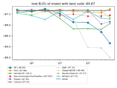
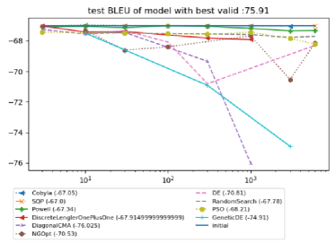
BLEU: C++ $\to$ Java BLEU: Python $\to$ C++  

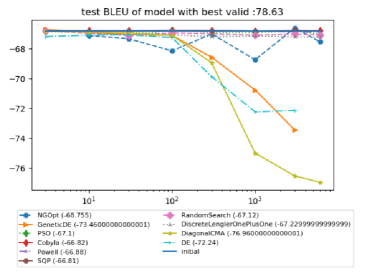
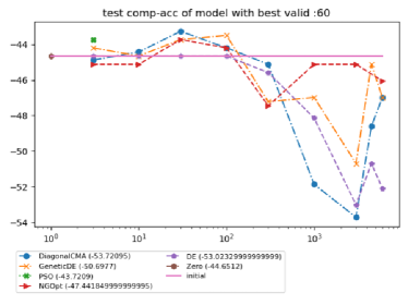
  BLEU: Python $\to$ Java Comp. accuracy: Python $\to$ Java  

Figure 3. Results of AfterLearnER on several problems from  (Roziere et al., 2020) with BLEU or Accuracy $\aleph$-losss (the lower the better). Each curve is the average over 3 runs of AfterLearner with a single optimization method in parameter $O$ of Algorithm 2, and the horizontal line is the baseline, i.e., without any retrofitting. AfterLearnER improves the result whatever the black-box optimizer used, though DiagonalCMA performs well on average.

5.4.4. Results: AfterLearnER can code

Figure 3 compares the solutions obtained using AfterLearnER (with different black-box optimizers $o$) to the baseline solution using a feedback limited to $b$ ground truth scalar numbers ($b$ on the $x$-axis). $O$ is restricted to a singleton $\{o\}$ (see $o$ in the legend) and a single run ($k=1$).

The results obtained with AfterLearER improve over the baseline whatever the optimizer used, though some optimizer perform better than others. Empirically, DiagonalCMA is often the best choice in this context.

5.4.5. Discussion

These experiments have been performed with the distribution of test cases in the original code from (Roziere et al., 2020), i.e., limit at 100: we investigated the case of a limit 512, but further work is needed on the dataset as there are redundancies between valid and test in that context (in particular when using computational accuracy, which aggregates distinct but functionally similar codes).

5.5. EG3D-cats: learning and optimizing in the latent space, unconditional case

5.5.1. Context: Offline optimization of the latent variable thanks to a surrogate model

EG3D-cats (Chan et al., 2022) is a pioneering work in 3D GANs, with impressive results. In the present Section, we improve EG3D-cats by learning the latent space: instead of randomly drawing a latent variable $z$, we learn a surrogate model of image quality and use it to optimize the input $z$ to the GAN, in order to get rid of bad $z$’s.

Building the surrogate model

We proceed as follows:

• Generate 200 images, corresponding to 200 randomly chosen latent variables $z$.

• Get binary user feedback: good or bad, for each image.

• Train a decision tree (we use the scikit-learn implementation (Pedregosa et al., 2011)) to approximate the probability, for a given latent variable $z$, that it generates a bad image: $tree(z)\approx P\left(bad|z\right)$.

5.5.2. $\aleph$-parameters:

The latent variable $z$ of EG3D-cats.

5.5.3. $\aleph$-loss: The surrogate model

We propose two variants of the algorithm, both using the trained decision tree described above to optimize the $\aleph$-parameters $z$:

• The random search variant applies random search on $tree$: Randomly draw $z$ until $tree(z)=0$, i.e. the trained decision tree predicts that the image will be ok.

• The evolutionary version applies NGOpt on the objective function $l:x\mapsto tree(z_{0}+\epsilon\cdot x)$ for some randomly drawn $z_{0}$. For a small $\epsilon$ (e.g., $1\mathrm{e}{-2}$), the final value is close to the starting point $z_{0}$, thus preserving the diversity of the original GAN: this is the main advantage of the evolutionary version compared to the random search.

To evaluate the approach, we use human raters to assess the improvement between initial $z$ and optimized $z$. The humans (not working in the computer science field) are presented with a cat generated by EG3D-cats and a cat generated by AfterLearnER: they choose the cat image they prefer, or click on “no preference”. The success rates are evaluated among cases in which they do have a preference. For the evolutionary variant, raters have to choose one of both cat images, but only images for which the initial $z_{0}$ was not satisfactory (i.e. $P(bad|z_{0})>0$) are presented: these statistical comparisons are based on paired data, i.e., $z_{0}$ vs $z_{0}+\epsilon\cdot x^{\star}$ with $x^{\star}$ recommended by the optimization run. Figures 4 and 5 present some qualitative results of before and after the evolution done by AfterLearnER.

5.5.4. Results: offline improvement of the model

The results are presented in Table 6. In all setups, we observe an improvement when using AfterLearnER compared to vanilla EG3D (i.e. all numbers are larger than $50\%$). Of course, the different random seeds used for computing these statistics are distinct from those used for creating the training set of 200 images.

Table 6. Results of the evolutionary version of the EG3D-cats algorithm with human raters, using a double-blind interface with randomized left/right positioning of compared images: the percentage shows how frequently our method outperformed the vanilla LDM according to human raters.

Initial model	Proposed method	Frequency of improvement $(\uparrow)$	Remark
afhqcats512-128	Random search	65% (160 images)	Cats
afhqcats512-128	Evolution	71% (193 images)	Cats

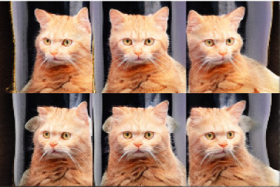
Figure 4. Example of evolution: unmodified cat (bottom) generated by EG3D-cats, and its evolutionary counterpart (top). Left: the ears have been significantly improved, while the neck is improved on the right.

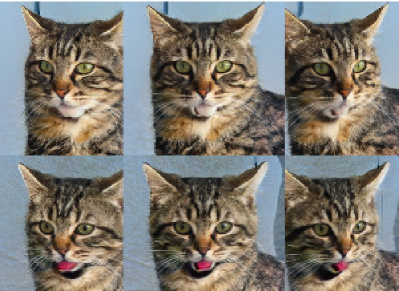
Figure 5. Example of evolution: unmodified cat (bottom) generated by EG3D-cats, and its evolutionary counterpart (top). In both cases, the mouth has been significantly modified, though it is still not perfect.

5.5.5. Discussion

We demonstrated that it is possible to learn a good approximation of the set of $z$’s that lead to errors using a decision tree, at a reasonable cost: labelling 200 examples is feasible for a motivated human.

5.6. LDM: learning and optimizing in the latent space, conditional case

5.6.1. Context: Using feedback to steer model output towards human preferences.

LDM (Rombach et al., 2022) provided impressive results in text to image generation recently: a prompt conditions the output. This section is based on (Videau et al., 2023), and applies the same techniques as in Section 5.5, on latent models in the present section.

Building the surrogate model

• Generate 200 images on the prompt “a photograph of an astronaut riding a horse”.

• Get a binary user feedback: good or bad, with a special emphasis on the quality of crops.

• Train a classifier (a decision tree or a neural network, and we use the scikit-learn implementation for both (Pedregosa et al., 2011) ) to approximate the probability, for a given latent variable $z$, that it generates a bad image: $tree(z)\simeq P\left(bad|z\right)$.

5.6.2. $\aleph$-parameters

The latent variable of LDM.

5.6.3. $\aleph$-loss: The Surrogate Model

As in Section 5.5.1, we use the trained decision tree as AfterLearnER $\aleph$-loss to determine an optimal latent value $z$, optimizing $z$ to minimize $tree(z)\approx P\left(bad|z\right)$. We stop the optimization as soon as we reach some $z$ satisfying $tree\left(z\right)=0$.

To assess the effectiveness of this approach, we rely on human raters. Specifically, raters are asked: “Is the crop of this image of top quality and does it include the entire astronaut and horse?” We refer to this evaluation metric as the ’satisfaction rate’.

5.6.4. Results

The results are presented in Table 7. We observe progress in all contexts: the frequency of poorly cropped images dramatically decreases.

Table 7. Results of AfterLearnER on LDM. The training is made on data labelled by us, and the performance here is on other generated images with/without AfterLearner, with different seeds. Some human raters, randomized order among the 4 tested methods, double-blind, prompt “A photograph of an astronaut riding a horse”. Between parenthesis the number of rated images. The overall comparison LDM vs. AfterLearnER+LDM is statistically significant, with p-value 0.04 for Fisher’s exact test. The ’satisfaction rate’ is described in Section 5.6.3.

Experimental setup	Optimizer	Loss	Satisfaction rate $(\uparrow)$
LDM			2.9% (486)
LDM+AfterLearnER	Random search	Decision tree	5.1 % (98)
LDM+AfterLearnER	Lengler	Decision tree	5.6 % (180)
LDM+AfterLearnER	Discrete$(1+1)$	Neural net	6.7 % (104)
Average LDM+AfterLearnER			5.7 % (382)

5.6.5. Discussion:

This success looks surprising: how can we learn something with 200 examples, whereas the latent space has size $4\cdot 64\cdot 64$? Nevertheless, the next section will confirm these results, switching to an online context, with an even lower budget.

5.7. LDM with online human feedback, learning from 15 images

5.7.1. Context:

In order to double-check the results above (successful inference from a few data points in a huge latent space), we perform the following experiment:

• 15 images are generated with the same text input.

• The users select their five favorite images.

• Learning a “local” surrogate model on the fly: these 5 favorite images are separated from the other 10, using scikit-learn neural network.

• Similarly to both previous sections, we minimize the probability of generating bad images (according to the local surrogate model) using Nevergrad (Lengler algorithm (Doerr et al., 2019)), with an initial point created by crossover (from (Videau et al., 2023) and specified below).

The crossover operator

The vanilla optimization by Nevergrad is here improved by creating a starting point for the optimization run built using a specific crossover operator, so-called Voronoi crossover (Hamda et al., 2002; Seo and Moon, 2002; Pehlivanoglu, 2012; Seo et al., 2005; Videau et al., 2023), in order to provide a better merging between different individuals than by geometric averages: the Voronoi split between $z_{1}$ and $z_{2}$ for getting a child corresponding to a crossover between images with latent variables $z_{1}$ and $z_{2}$ (Algorithm 3). These Voronoi combinations are used as starting points for the optimization by AfterLearnER.

Latent variables $z_{1}$ and $z_{2}$, coordinates $p_{1}\in I_{1}=LDM(z_{1})$ and $p_{2}\in I_{2}=LDM(z_{2})$.

Create a new latent variable $z$ of same shape as $z_{1}$ and $z_{2}$.

for each $p$ spatial coordinate in $z$. do

     if $||p_{1}-p||<||p_{2}-p||$ then

         $z(p)=z_{1}(p)$

     else

         $z(p)=z_{2}(p)$

     end if

end for

Algorithm 3 Crossover between images with latent variables $z_{1}$ and $z_{2}$, at points $p_{1}$ and $p_{2}$. Here the user has selected the point $p_{1}$ in the image generated from the latent variable $z_{1}$ and the point $p_{2}$ in the image generated from the latent variable $z_{2}$, out of 15 images. Latent variables are tensors with shape $64\times 64\times 4$.

Application of the crossover operator for more than 2 clicks by users

Two modifications of Algorithm 3 are needed. First, we might have more than 2 images chosen by the user, so we extend Algorithm 3 to more than two images. Second, we need to create more than one offspring, so that a randomization is necessary. For these two extensions, we follow (Videau et al., 2023): let us consider $k$ clicks, with positions $p_{1},\dots,p_{k}$, in images built on latent variables $z_{i_{1}},\dots,z_{i_{k}}$. Each offspring image $I_{Voronoi}=G(z_{Voronoi})$ is built by constructing a latent variable $z_{Voronoi}$ as in Figures 1-3.

(1) $$r \mbox{ is randomly drawn uniformly in }[1,2]$$

(2) $$z_{Voronoi}(x) = z_{i_{j}}(x)\mbox{ if }\ \forall u\neq j,||x-p_{j}||<\frac{1}{r}||x-p_{u}||$$

(3) $$z_{Voronoi}(x) \sim \mathcal{N}(0,\,1)\mbox{for each channel otherwise}$$

5.7.2. $\aleph$-loss

To evaluate this approach, we use a specific prompt and quality criteria (see below). We generate a batch of images with the vanilla LDM, and a second batch, using AfterLearnER, after selection of the 5 best by the user.

We then compare the number of images that fit the given criteria in the initial batch (no user feedback) and in subsequent batches (i.e., with user feedback).

5.7.3. Results

AfterLearnER was tested on three different setups:

• First setup: the prompt is “A close up photographic portrait of a young woman with colored hair.”. We consider images 15 to 28, in 2 cases: first case, the user selects red hair; and second case, the user selects blue hair. Observation: the next generation by AfterLearnER + LDM have dramatically greater proportions of red hair (resp. blue hair).

• Second context: “fighting Cthulhu in the jungle”. For the second setup (Figure 6), we present more sophisticated experiments with celebrities fighting Cthulhu. We observe a moderate improvement, on this easy setting of very famous people: some people, like X Y (anonymized celebrity), are easier to generate in arbitrary contexts, so that the classical LDM performs well. The prompt becomes much harder for a scientist like Yann LeCun: the improvement becomes much greater. we do this in Figure 7 and the improvement is stronger.

• Third setup, we now check that AfterLearnER can also have an impact on realism. We just ask for “Medusa” and feed AfterLearnER with the realism opinion of the user. The second batch uses preferences mentioned by the user in the first batch, then the third batch uses preferences mentioned by the user in the second batch, and so on. Each batch improves over the previous one. Within 3 batches of 14 images, we get way more realistic portraits of Medusa (Figure 8).

Results are aggregated in Table 8. They are always positive, with a clear gap in 3 out of 4 contexts.

5.7.4. Discussion

In each setup, we increase the proportion of images that fit specific criteria. This approach is particularly effective for generating images that are difficult to produce by default, such as “Yann LeCun fighting tentacles in the Jungle”. In these challenging scenarios, the text-to-image model struggles to combine elements like Yann LeCun, a jungle, and tentacles. However, by selecting the right images, we can guide the model to produce outputs that better match user preferences, showing the effectiveness of the proposed approach.

Table 8. Overview of our low budget image generation experiments. FB refers to user feedback (clicks on the preferred images inside a screen presenting a batch of images). For  Figure 8 the quality is not measured by quantified metrics and the reader can compare the top 2 rows to the bottom 2 rows there.

Figure		Context	Observation
	Top	2nd batch, after FB	Mostly red hair
		on red hair in batch 1
	Bottom	2nd batch, after FB	All blue hair
		on blue hair in batch 1
	Top	Initial batch	Success 11/14
Fig.	Middle	Batch 2 after FB on batch 1	Success 12/14
6	Botom	Batch 3 after FB on	Success 13/14
		batches 1 and 2
Fig.	Top	Initial batch	Success $\simeq 30\%$
7	Bottom	After FB on the 1st batch	Success $\simeq 71\%$
Fig.	Top	Initial batch	Low quality
8	Middle	After FB on 1st batch
	Bottom	After FB on batches 1 and 2	High quality

First batch of 14 images. Tentacles: in 11 images. XY is the only human: in 12 images.

Second batch of 14 images. Tentacles in 12 images. XY is the only human: in all images.

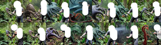
Third batch of 14 images. Tentacles: in 13 images. XY is the only human: in all images.

Figure 6. XXX YYY (anonymized) fighting tentacles in the jungle. The original LDM is already good here, but we observe an increased frequency of XXX YYY and an increased frequency of tentacles in the new batches. All images have significant differences in terms of position. A more challenging task is proposed in Figure 7.

Initial generations of 15 images, by the vanilla LDM code. Tentacles in 4 or 5 images, over 15: tentacles are difficult to obtain when a scientist is in the picture.

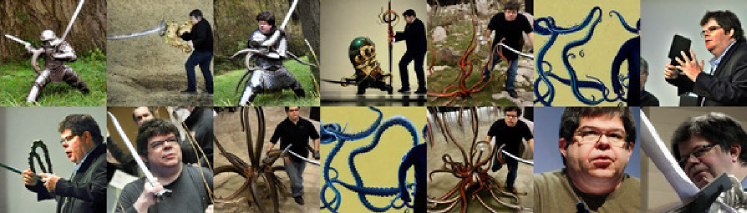
After selection of the 5 preferred images out of the 15 above, 14 new generations by AfterLearnER. Tentacles in 10/14 images.

Figure 7. A scientist fighting tentacles in the jungle. The frequency of tentacles has increased a lot. All images have significant differences in terms of position. We observe again that 15 images evaluated by the user are enough for a meaningful impact.

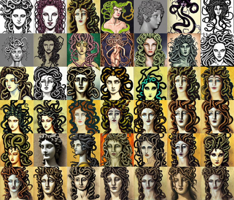
Figure 8. Medusa. Top two rows: first batch, i.e., equivalent to default LDM. Rows 3 and 4: second generation, after clicking on the most realistic image of the first batch. Rows 5 and 6: generation 3, after clicking on the two most realistic images of generation 2. Colors become better, and sus-sternal dimples appear. We observe that a user feedback about 2 generations of images are enough for improving outputs.

6. Overview and discussion

All results in the present paper come from applying AfterLearnER after a classical ML pipeline.

Depth sensing: We use the small MiDaS model and optimize $\aleph$-parameters on a small dataset. More precisely, 300 images are used for optimizing $\aleph$-parameters by distillation of the big MiDaS model so that we get test errors better than the original Small MiDaS, or even (in some cases) the Hybrid MiDaS. These results only require 50 scalars of feedback for adapting a model to different loss functions. In this benchmark, the loss is not differentiable either.

Speech resynthesis: We use the checkpoint previously tuned in  (Kharitonov et al., 2022) and optimize two $\aleph$-parameters on 75% of the test set and check on the remaining test data. This is a simple experiment with just two constants, hardcoded in the original code, optimized on a small dataset. The numbers are not directly comparable to the original work as we use a split of the test set: but we show that a small feedback (40 scalars) on a split of the test set is enough for, on average, an improvement on the rest of the test set. Compared to (Ranzato et al., 2016), we do a fast distribution shift and not a whole training.

Doom/Arnold: In this reinforcement learning context, we use the same simulator as the one used in the original paper/code. This consistency allows for a direct comparison of our results. We observed enhanced outcomes primarily because we focused on optimizing the actual objective function.

Transcoder: We use the same training/validation data as in the GitHub repository of (Roziere et al., 2020). We immediately observe an improvement (Figure 3) only using a few hundred scalars. We do not use any information about the objective function, so we could have an online estimator such as speed, memory consumption or elegance — which cannot be done with the original supervised learning.

3D Gan EG3D for AFHQ (cats): With 200 feedbacks, we built a more realistic EG3D-cats, outperforming state-of-the-art in three-dimensional cats.

LDM: We provide an interactive counterpart of LDM. The fact that it works is quite counter-intuitive: the latent space has dimension $4\cdot 64\cdot 64$. We perform several tests with hair color, image quality, and realism, and results are precise. They are in line with user needs: whereas most LDM users (in particular in the new field of prompt engineering for txt2img) do many independent rerolls, we guide these rerolls using previous results.

A further work would be removing the significant engineering work necessary for reward shaping thanks to AfterLearnER.

7. Conclusions

This paper demonstrates the potential of integrating small-scale feedback directly into the optimization process, as in retrofitting, through black-box optimization approaches. Likewise, such a strategy is especially beneficial for optimizing, with a few scalars, a non-differentiable criteria, a common challenge in various fields. That way, we provide substantial improvements in state-of-the-art DL applications, e.g., in scenarios such as Doom and code translation. Furthermore, our methodology enables the generation images with minimal user interaction, requiring as few as three interactions for getting a first approximation. Similarly, we optimize $\aleph$-parameters for depth estimation, language translation, and speech synthesis. Our method requires only dozens to hundreds of (e.g., human) evaluations to achieve significant improvements. Additionally, we have enhanced the EG3D-cats model with a streamlined codebase, illustrating our approach’s versatility and practicality (see Algorithm 4). Overall, our findings underscore the value of human-in-the-loop methodologies or simulation-based feedbacks in refining DL solutions across various domains, without relying on millions of feedbacks.

⬇

# Code for modifying a latent vector z, using a list of the

# bad random seeds over the 200 first seeds.

if ”afhqcats512-128” in network_pkl:

Y = [1] * 200 # Seeds 15, 84, 47 are bad for cats.

bad_latent_z = [15,84,47,30,33,78,4,50,49,

56,11,17, 36,85,59,16,63,81,25,39,

87,45,41,58,60,68,46,38]

bad_latent_z += [130,113,146,107,143,

175,158,192,121,

110,181,186,170,120,163,193,155,

144,148,191,141, 105,187,183,174,

129,117,100,157,166,194,198,138,

156,168,114,127,103,109]

if ”ffhqrebalanced512-64” in network_pkl:

Y = [1] * 200

bad_latent_z = [27,14,88,42,37,25,73,

53,40,17,45,92,

50,3,84,29,12,31,98,72,51,46,57,16,13,33,

43,69,60,74, 77,75,41,89,39,87,68,67,56,

35,26,9,23,7,38,20,63,55,

28,36,8,6,64]

bad_latent_z += [132,145,194,187,119,169,

137,176,185, 147,111,139,171,

101,161,116,115,155,175,118,112,144,172,

198,124,181, 129,117,189,108,174,138,121,143,

156,130,146,179,140,153,136,168,131,180,110,

109,199,100]

for p in bad_latent_z:

Y[p] = 0

X = [list(np.random.RandomState(i).randn(1, G.z_dim)[0])

for i in range(len(Y))]

# Learning with Scikit-Learn.

from sklearn import tree

clf = tree.DecisionTreeClassifier()

print(len(X), len(Y), len(X[0]))

clf = clf.fit(X, Y)

# Optimization with Nevergrad.

z = np.random.RandomState(seed).randn(1, G.z_dim)

import nevergrad as ng

epsilon = 0.01

def loss(x):

assert len(x) == G.z_dim

return clf.predict_proba(

[list(z[0] + epsilon * x)])[0][0]

nevergrad_optimizer = ng.optimizers.NGOpt(

G.z_dim, 10000)

for nevergrad_iteration in range(1, 10000):

x = nevergrad_optimizer.ask()

l = loss(x.value)

if l < 1e-5:

break

else:

nevergrad_optimizer.tell(x, l)

print(f”Success␣in␣{nevergrad_iteration}␣iterations”)

z[0] += epsilon * nevergrad_optimizer.recommend().value

Algorithm 4 The short code at the top of EG3D-cats for getting AfterLearnER on top of it. There is no significant computational overhead, we learn directly from $z$: we do not have to generate anything.

We recommend employing AfterLearnER in the following scenarios:

• Consider problems in which the actual objective is not differentiable, and is hence typically approximated for gradient-based training by various proxies, or by ad-hoc reward shaping.

• Black-box retrofitting must come after the classical gradient-based training, and without any backprop retraining.

• Restrict the $\aleph$-parameters to key parameters: typically, some parameters at the input or output transformations, or a single layer as small as possible. Dimensions in the 1000s is manageable in a black-box manner (though this depends on the budget of course), but prefer as much as possible small families of parameters that intersect all paths from input to output.

• Increasing the number of runs (parameter $k$), or the parallelism $\lambda$, makes the code closer to random search, and less prone to overfitting, as confirmed by the theoretical analysis of Section 4.2. A relatively low budget is sufficient, both in terms of number of feedbacks (whereas most papers use dozens of thousands to hundreds of thousands of scalar feedbacks), and computational cost: a value of $k=1$ has frequently been used here, except for Doom for which we mostly set $k=30$.

We emphasize the concept of small aggregated anytime feedback (SAAF). While we did a part of our experiments from automatically computed feedback (e.g., word error rate based on programs for speech synthesis or the biggest MiDaS model in depth estimation), AfterLearnER uses an aggregated feedback, which could be provided by humans, based on a global experience of the system, without the need for fine grain feedback. Also, this shows a clear generalization: compared to systems using millions of fine-grained feedback, our system can not so easily “cheat” (overfit) using redundancies between train/validation and test.

Limitations and further work

Most of the feature construction was performed by DL: what we propose can be added on top of a DL solution, but does not replace it. We outperform Arnold for Doom, but only with Arnold and its reward shaping as an excellent starting point. The situation is similar for speech resynthesis, interactive generation and depth sensing. In the case of the Transcoder, we manage to optimize a few weights of the checkpoint within a few dozens evaluations.

Maybe some of our results could be improved by applying AfterLearnER on several layers in turn: in the present paper we just heuristically guessed which parameters to optimize, and did not investigate bigger search spaces. This might be particularly true for cases in which we can generate new data with a simulator, as in the case of Doom.

Improving generalization by searching for flat optima is a challenging topic (He et al., 2019; Baldassi et al., 2020; Hoffer et al., 2017), mostly explored for gradient-based optimization of weights: our context (black-box optimization, validation set, after training) is specific, promising, and deserves exploration. This includes the mathematics in Section 4.2, inspired from (Fournier and Teytaud, 2011).

Multi-objective extensions seem to be natural for Arnold/Doom (using the various reward shaping criteria used in the original code) and for code translation, where BLEU and comp. acc. are completely different measures, and for the many criteria of depth sensing.

The present paper demonstrated the applicability of AfterLearnER, with experiments reproducible with a relatively low budget. A natural next step is the large scale application on unsolved problems, such as hallucinations in large language models or code translation optimized for speed.

Appendix A Full results for the AfterLearnER / MiDaS experiment

We observe here (i) good performance even with a low budget (total budget $<300$ is enough for positive results) (ii) good transfer, in particular when training on Th3.

For each budget, there are three loss functions Th1, Th2 and Th3 which can be used in training or in test, hence 9 curves. For 3 of them, train and test use the same loss function: the 6 others are about transfer. The non-transfer cases are also presented in the main text. Fig. 9 consider a budget $b=1$. Fig. 10 considers a budget $b=50$. Fig. 11 considers a budget 150. In each figure, the x-axis is the number of runs $k$.

Testing on Th1, training with Th1, Th2, Th3 respectively:

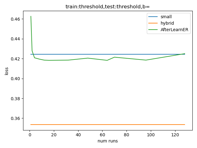
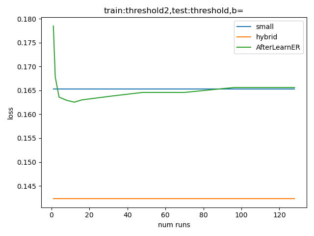
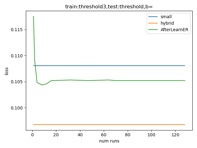
Testing on Th2, training with Th1, Th2, Th3 respectively:

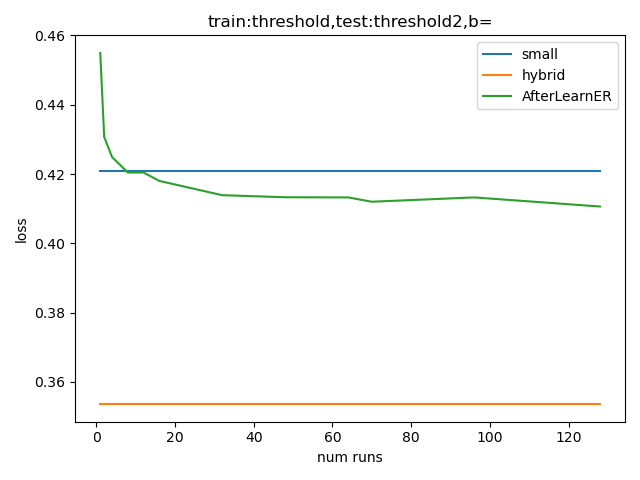
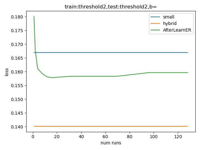
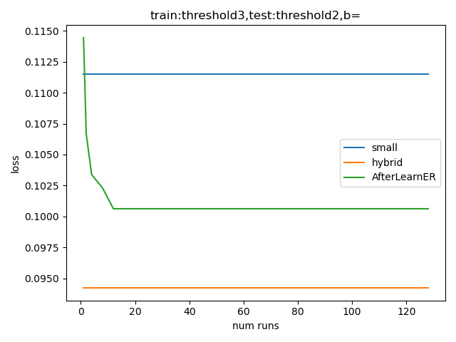
Testing on Th3, training with Th1, Th2, Th3 respectively:

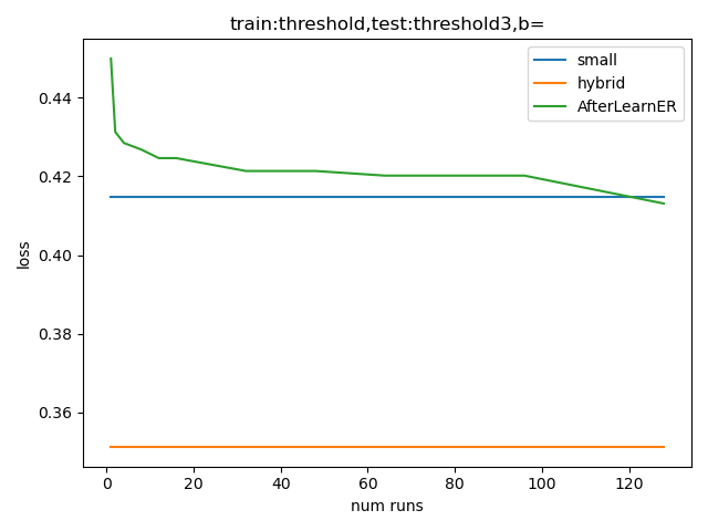
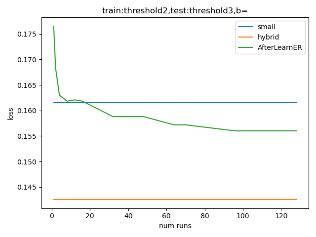
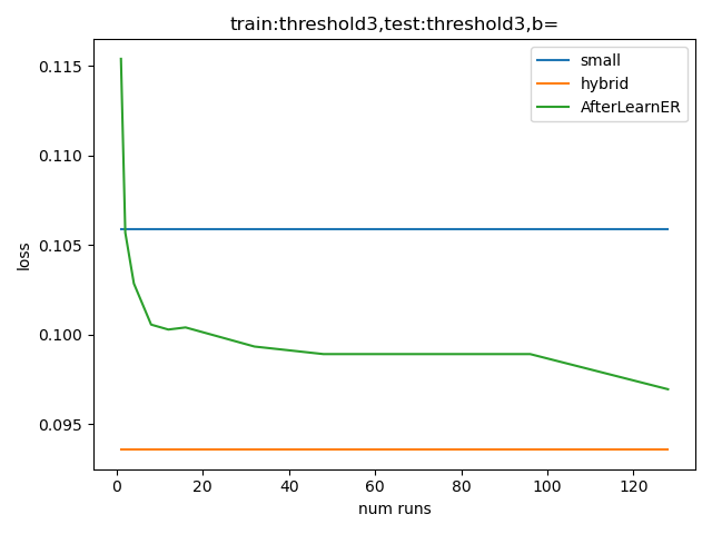
Figure 9. AfterLearnER applied to MiDaS with budget $B=\{1\}$: with this budget 1, we are actually running random search and already get positive results. We note that with a training on Th3, we get positive results for all tests with $b\times k$ (total number of scalar evaluations provided to AfterLearner) less than 20: so 20 evaluations is enough for a good transfer to all criteria Th1, Th2, Th3.

Testing on Th1, training with Th1, Th2, Th3 respectively:

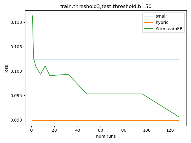
Testing on Th2, training with Th1, Th2, Th3 respectively:

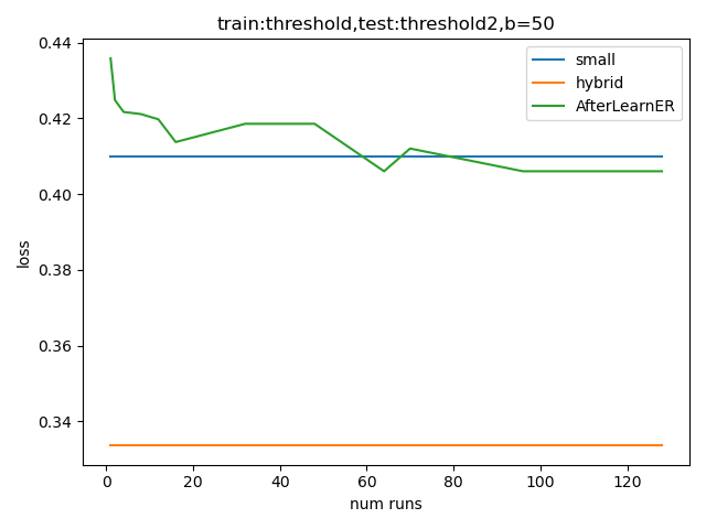
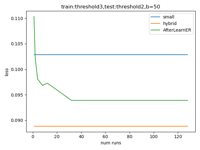
Testing on Th3, training with Th1, Th2, Th3 respectively:

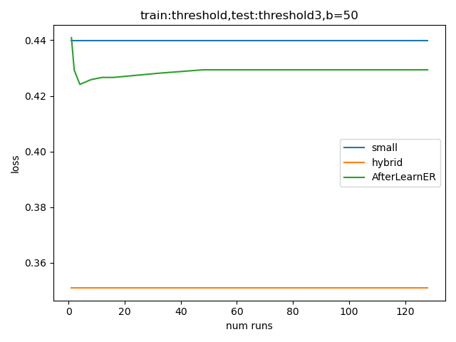
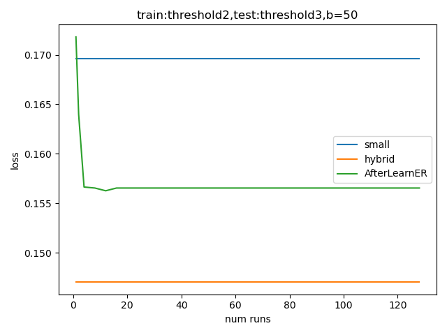
Figure 10. AfterLearnER applied to MiDaS with budget $B=\{50\}$. Compared to $B=\{1\}$, the number of scalar evaluations needed for beating the baseline is greater, but remains in the hundreds. Th3 remains the best training criterion for good transfer to all 3 criteria Th1,Th2,Th3.

Testing on Th1, training with Th1, Th2, Th3 respectively:

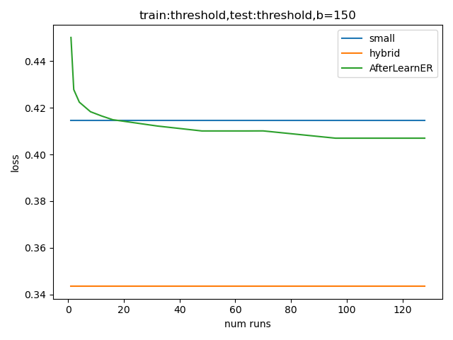
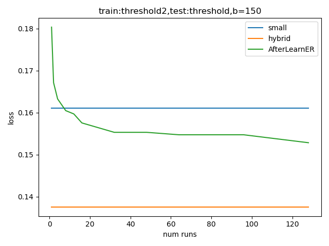
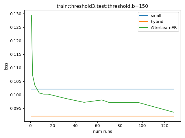
Testing on Th2, training with Th1, Th2, Th3 respectively:

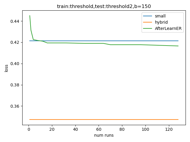
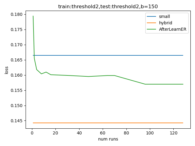
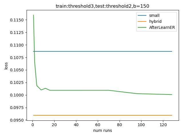
Testing on Th3, training with Th1, Th2, Th3 respectively:

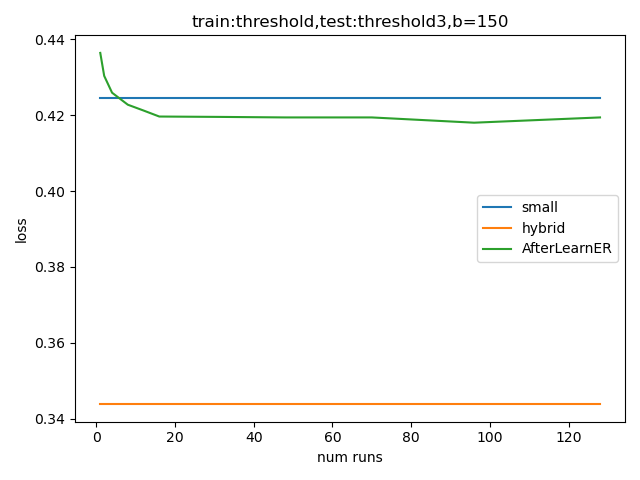
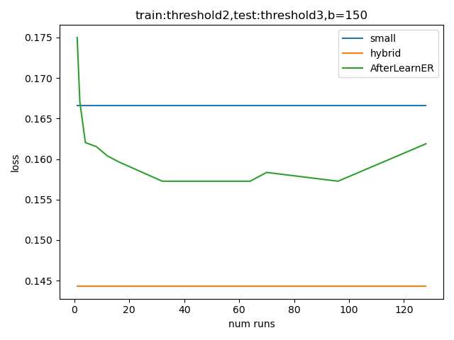
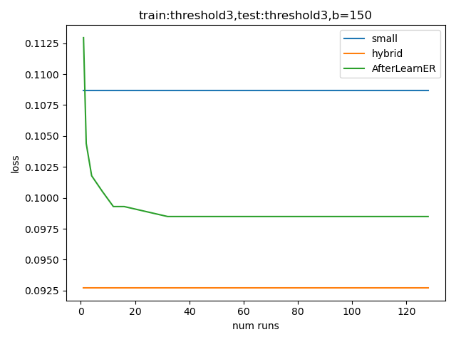
Figure 11. AfterLearnER applied to MiDaS with budget $B=\{150\}$. Compared to $B=\{1\}$, the number of scalar evaluations needed for beating the baseline is greater, but remains in the hundreds. Th3 remains the best training criterion for good transfer to all 3 criteria Th1,Th2,Th3.

Appendix B Black-box optimization wizards and NGOpt

After becoming famous in SAT solving(Xu et al., 2008), wizards become important in black-box optimization as well(Weise et al., 2018; Liu et al., 2020; Awad et al., 2020; Meunier et al., 2022a).

Optimization wizards are based on selecting, from characteristics of the domain (dimension, type of variables) and of the optimization run (budget, parallelism), an optimization algorithm or a bet-and-run (Weise et al., 2018) or chaining of several optimization algorithms. NGOpt, an open source wizard for black-box optimization, is available in (Rapin and Teytaud, 2018) and as a PyPi package.

For example, in a continuous setting, with moderate dimension and a large budget and a sequential optimization context (no parallelism), NGOpt(Meunier et al., 2022a) chooses a chaining of CMA(Hansen and Ostermeier, 2003) fastened with a metamodel and followed by Sequential Quadratic Programming(Artelys, 2015).

An example of code involving NGOpt is provided in Appendix C.

Appendix C Reproducibility

All black-box optimization algorithms are available in (Rapin and Teytaud, 2018). Nevergrad can be installed by cloning https://github.com/facebookresearch/nevergrad or by “pip install nevergrad”.

A minimal example of optimization with some optimization methods mentioned above is in Algorithm 5.

Algorithm 5 Minimal example of black-box optimization.

⬇

import nevergrad as ng

import numpy as np

def loss(x):

return np.sum((x - 1.7) ** 2)

# 3 optimization methods in dimension 10, continuous.

optim_ngopt = ng.optimizers.registry[”NGOpt”](10, 500)

optim_de = ng.optimizers.registry[”DE”](10, 500)

optim_lengler= ng.optimizers.registry[”DiscreteLenglerOnePlusOne”](10, 500)

# 1 optimization method for dimension 10, integer values between 1 and 4,

# with 30 parallel evaluations.

array = ng.p.Array(init=np.array([2] * 10), lower=1, upper=4).set_integer_casting()

optim_opo = ng.optimizers.registry[”DiscreteOnePlusOne”](array, 500)

# an example with minimize

print(optim_ngopt.minimize(lambda x: loss(x)).value)

# an example with ask and tell

for k in range(50):

x = optim_de.ask()

y = loss(x.value)

optim_de.tell(x, y)

# an example with minimize in a discrete context

print(optim_opo.minimize(loss).value)

The detailed code for improving EG3D is in Algorithm 4.

Appendix D Computational cost

Table 9. Computational cost. *Here the cost is in terms of data collection. **We get positive results even with very low budget, though greater budgets lead to better results (Figure 3). The online overhead exists only when we modify, online, the latent variables of a GAN for each new generation of images: however, it is typically negligible compared to the generation of images itself.

Application	computational cost
	Offline comp. cost	Online overhead
Depth sensing
(Fig. 2, $k=10$, $B=50$)	12h, 10 GPUs	zero
Speech resynthesis (Tab. 4, 1st line)	1 GPU, 2 hours	zero
EG3D	200 labelled examples*	negligible
LDM (offline, Section 5.6)	200 images	negligible
LDM (online, Section 5.7)	negligible	negligible
Doom (Tab. 5)	48 hours, $k$ GPU	zero
Code translation	0 to 54 hours**,	zero
	0 to thousands of ^
	^ labelled translations

Table 9 presents typical computational costs of AfterLearnER, for a typical entire run providing significant improvements compared to the initial DL tool.

References

- (1)
- Abramson et al. (2022) Josh Abramson, Arun Ahuja, Federico Carnevale, Petko Georgiev, Alex Goldin, Alden Hung, Jessica Landon, Jirka Lhotka, Timothy Lillicrap, Alistair Muldal, George Powell, Adam Santoro, Guy Scully, Sanjana Srivastava, Tamara von Glehn, Greg Wayne, Nathaniel Wong, Chen Yan, and Rui Zhu. 2022. Improving Multimodal Interactive Agents with Reinforcement Learning from Human Feedback. arXiv:2211.11602 [cs.LG]
- Adams et al. (2022) Stephen Adams, Tyler Cody, and Peter A. Beling. 2022. A survey of inverse reinforcement learning. Artif. Intell. Rev. 55, 6 (aug 2022), 4307–4346. https://doi.org/10.1007/s10462-021-10108-x
- Arakawa et al. (2018) Riku Arakawa, Sosuke Kobayashi, Yuya Unno, Yuta Tsuboi, and Shin-ichi Maeda. 2018. Dqn-tamer: Human-in-the-loop reinforcement learning with intractable feedback. arXiv:1810.11748 (2018).
- Artelys (2015) SME Artelys. 2015. Artelys SQP Wins the BBCOMP competition. https://www.ini.rub.de/PEOPLE/glasmtbl/projects/bbcomp/index.html.
- Assunção et al. (2019) Filipe Assunção, Nuno Lourenço, Penousal Machado, and Bernardete Ribeiro. 2019. DENSER: Deep Evolutionary Network Structured Representation. Genetic Programming and Evolvable Machines 20 (03 2019).
- Awad et al. (2020) Noor Awad, Gresa Shala, Difan Deng, Neeratyoy Mallik, Matthias Feurer, Katharina Eggensperger, Andre’ Biedenkapp, Diederick Vermetten, Hao Wang, Carola Doerr, Marius Lindauer, and Frank Hutter. 2020. Squirrel: A Switching Hyperparameter Optimizer. arXiv:2012.08180 [cs.LG]
- Baevski et al. (2020) Alexei Baevski, Yuhao Zhou, Abdelrahman Mohamed, and Michael Auli. 2020. wav2vec 2.0: A framework for self-supervised learning of speech representations. Advances in neural information processing systems 33 (2020), 12449–12460.
- Baldassi et al. (2020) Carlo Baldassi, Enrico M. Malatesta, Matteo Negri, and Riccardo Zecchina. 2020. Wide flat minima and optimal generalization in classifying high-dimensional Gaussian mixtures. arXiv:2010.14761 (2020).
- Beyer (1998) Hans-Georg Beyer. 1998. Mutate large, but inherit small! On the analysis of rescaled mutations in ( -ES with noisy fitness data. In Parallel Problem Solving from Nature — PPSN V. Springer, 109–118.
- Birkl et al. (2023) Reiner Birkl, Diana Wofk, and Matthias Müller. 2023. Midas v3. 1–a model zoo for robust monocular relative depth estimation. arXiv preprint arXiv:2307.14460 (2023).
- Bonferroni (1936) Carlo Bonferroni. 1936. Teoria statistica delle classi e calcolo delle probabilita. Pubblicazioni del R Istituto Superiore di Scienze Economiche e Commericiali di Firenze 8 (1936), 3–62.
- Burkholz (2024) Rebekka Burkholz. 2024. Batch normalization is sufficient for universal function approximation in CNNs. In The Twelfth International Conference on Learning Representations. https://openreview.net/forum?id=wOSYMHfENq
- Chan et al. (2022) Eric R. Chan, Connor Z. Lin, Matthew A. Chan, Koki Nagano, Boxiao Pan, Shalini De Mello, Orazio Gallo, Leonidas Guibas, Jonathan Tremblay, Sameh Khamis, Tero Karras, and Gordon Wetzstein. 2022. Efficient Geometry-aware 3D Generative Adversarial Networks. In CVPR.
- Chen et al. (2022) Dian Chen, Dequan Wang, Trevor Darrell, and Sayna Ebrahimi. 2022. Contrastive Test-Time Adaptation. In IEEE/CVF Conference on Computer Vision and Pattern Recognition. 295–305.
- Chiu et al. (2019) Billy Chiu, Simon Baker, Martha Palmer, and Anna Korhonen. 2019. Enhancing biomedical word embeddings by retrofitting to verb clusters. In BioNLP@ACL. https://api.semanticscholar.org/CorpusID:199379311
- Dang and Lehre (2016) Duc-Cuong Dang and Per Kristian Lehre. 2016. Self-adaptation of Mutation Rates in Non-elitist Populations. In Parallel Problem Solving from Nature - PPSN XIV - 14th International Conference. 803–813.
- Dawson (2007) Richard Dawson. 2007. Re-engineering cities: a framework for adaptation to global change. Philosophical Transactions of the Royal Society A: Mathematical, Physical and Engineering Sciences 365, 1861 (2007), 3085–3098.
- Dixon and Eames (2013) Tim Dixon and Malcolm Eames. 2013. Scaling up: the challenges of urban retrofit. Building research & information 41, 5 (2013), 499–503.
- Doerr et al. (2019) Benjamin Doerr, Carola Doerr, and Johannes Lengler. 2019. Self-Adjusting Mutation Rates with Provably Optimal Success Rules. In Proceedings of the Genetic and Evolutionary Computation Conference (GECCO ’19). Association for Computing Machinery, 1479–1487.
- Douglas (2006) James Douglas. 2006. Building adaptation. Routledge.
- Eiben and Smith (2015) A. E. Eiben and James E. Smith. 2015. Introduction to Evolutionary Computing (2nd ed.). Springer.
- Faruqui et al. (2015a) Manaal Faruqui, Jesse Dodge, Sujay Kumar Jauhar, Chris Dyer, Eduard Hovy, and Noah A. Smith. 2015a. Retrofitting Word Vectors to Semantic Lexicons. In Conference of the North American Chapter of the Association for Computational Linguistics: Human Language Technologies, Rada Mihalcea, Joyce Chai, and Anoop Sarkar (Eds.). 1606–1615.
- Faruqui et al. (2015b) Manaal Faruqui, Jesse Dodge, Sujay Kumar Jauhar, Chris Dyer, Eduard Hovy, and Noah A. Smith. 2015b. Retrofitting Word Vectors to Semantic Lexicons. In Conference of the North American Chapter of the Association for Computational Linguistics: Human Language Technologies, Rada Mihalcea, Joyce Chai, and Anoop Sarkar (Eds.). 1606–1615.
- Feurer and Hutter (2019) Matthias Feurer and Frank Hutter. 2019. Hyperparameter optimization. In Automated Machine Learning: Methods, Systems, Challenges, Frank Hutter, Lars Kotthoff, and Joaquin Vanschoren (Eds.). Springer Verlag, 3–38.
- Fournier and Teytaud (2011) Hervé Fournier and Olivier Teytaud. 2011. Lower Bounds for Comparison Based Evolution Strategies Using VC-dimension and Sign Patterns. Algorithmica 59, 3 (2011), 387–408.
- Giannou et al. (2023) Angeliki Giannou, Shashank Rajput, and Dimitris Papailiopoulos. 2023. The Expressive Power of Tuning Only the Normalization Layers. In The Thirty Sixth Annual Conference on Learning Theory, COLT 2023, 12-15 July 2023, Bangalore, India (Proceedings of Machine Learning Research, Vol. 195), Gergely Neu and Lorenzo Rosasco (Eds.). PMLR, 4130–4131. https://proceedings.mlr.press/v195/giannou23a.html
- Goyal et al. (2022) Sachin Goyal, Mingjie Sun, Aditi Raghunathan, and J. Zico Kolter. 2022. Test Time Adaptation via Conjugate Pseudo-labels. In Advances in Neural Information Processing Systems, S. Koyejo, S. Mohamed, A. Agarwal, D. Belgrave, K. Cho, and A. Oh (Eds.), Vol. 35. 6204–6218.
- Hamda et al. (2002) Hatem Hamda, François Jouve, Evelyne Lutton, Marc Schoenauer, and Michele Sebag. 2002. Compact unstructured representations for evolutionary design. Applied Intelligence 16 (2002), 139–155.
- Hansen and Ostermeier (2003) Nikolaus Hansen and Andreas Ostermeier. 2003. Completely Derandomized Self-Adaptation in Evolution Strategies. Evolutionary Computation 11, 1 (2003).
- He et al. (2019) Haowei He, Gao Huang, and Yang Yuan. 2019. Asymmetric Valleys: Beyond Sharp and Flat Local Minima. In Advances in Neural Information Processing Systems, H. Wallach, H. Larochelle, A. Beygelzimer, F. d'Alché-Buc, E. Fox, and R. Garnett (Eds.), Vol. 32.
- Hiranandani et al. (2021) Gaurush Hiranandani, Hari Narasimhan, Jatin Mathur, Mahdi Milani Fard, and Sanmi Koyejo. 2021. Optimizing Blackbox Metrics with Iterative Example Weighting. In 38th International Conference on Machine Learning.
- Hoffer et al. (2017) Elad Hoffer, Itay Hubara, and Daniel Soudry. 2017. Train Longer, Generalize Better: Closing the Generalization Gap in Large Batch Training of Neural Networks. In 31st International Conference on Neural Information Processing Systems. 1729–1739.
- Holland (1975) John H. Holland. 1975. Adaptation in Natural and Artificial Systems. University of Michigan Press.
- Huang et al. (2021) Chen Huang, Shuangfei Zhai, Pengsheng Guo, and Josh Susskind. 2021. MetricOpt: Learning To Optimize Black-Box Evaluation Metrics. In Proceedings of the IEEE/CVF Conference on Computer Vision and Pattern Recognition (CVPR). 174–183.
- Hwang et al. (2021) Seung-Jun Hwang, Sung-Jun Park, Gyu-Min Kim, and Joong-Hwan Baek. 2021. Unsupervised Monocular Depth Estimation for Colonoscope System Using Feedback Network. Sensors 21, 8 (2021).
- Jain et al. (2015) Ashesh Jain, Shikhar Sharma, Thorsten Joachims, and Ashutosh Saxena. 2015. Learning preferences for manipulation tasks from online coactive feedback. Int. J. Robotics Res. 34, 10 (2015), 1296–1313. https://doi.org/10.1177/0278364915581193
- Jiang et al. (2020) Qijia Jiang, Olaoluwa Adigun, Harikrishna Narasimhan, Mahdi Milani Fard, and Maya Gupta. 2020. Optimizing Black-box Metrics with Adaptive Surrogates. In Proceedings of the 37th International Conference on Machine Learning (Proceedings of Machine Learning Research, Vol. 119), Hal Daumé III and Aarti Singh (Eds.). PMLR, 4784–4793. https://proceedings.mlr.press/v119/jiang20a.html
- Jiao et al. (2023) Mingsheng Jiao, Tingrui Yu, Xuan Li, Guanjie Qiu, Xiaodong Gu, and Beijun Shen. 2023. On the Evaluation of Neural Code Translation: Taxonomy and Benchmark. arXiv:2308.08961
- Kandasamy et al. (2018) Kirthevasan Kandasamy, Willie Neiswanger, Jeff Schneider, Barnabás Póczos, and Eric P. Xing. 2018. Neural architecture search with Bayesian optimisation and optimal transport. In 32nd International Conference on Neural Information Processing Systems, Samy Bengio, Hanna M. Wallach, Hugo Larochelle, Kristen Grauman, and Nicolò Cesa-Bianchi (Eds.). 2020–2029.
- Kempka et al. (2016) Michał Kempka, Marek Wydmuch, Grzegorz Runc, Jakub Toczek, and Wojciech Jaśkowski. 2016. ViZDoom: A Doom-based AI Research Platform for Visual Reinforcement Learning. (2016). https://doi.org/10.48550/ARXIV.1605.02097
- Kennedy and Eberhart (1995) James Kennedy and Russell C. Eberhart. 1995. Particle swarm optimization. In Proceedings of the IEEE International Conference on Neural Networks. 1942–1948.
- Khalidov et al. (2019) Vasil Khalidov, Maxime Oquab, Jérémy Rapin, and Olivier Teytaud. 2019. Consistent population control: generate plenty of points, but with a bit of resampling. In Proceedings of the 15th ACM/SIGEVO Conference on Foundations of Genetic Algorithms, FOGA 2019, Potsdam, Germany, August 27-29, 2019. 116–123. https://doi.org/10.1145/3299904.3340312
- Kharitonov et al. (2022) Eugene Kharitonov, Jade Copet, Kushal Lakhotia, Tu Anh Nguyen, Paden Tomasello, Ann Lee, Ali Elkahky, Wei-Ning Hsu, Abdelrahman Mohamed, Emmanuel Dupoux, and Yossi Adi. 2022. textless-lib: a Library for Textless Spoken Language Processing. arXiv:2202.07359 (2022).
- Kim et al. (2023) Changyeon Kim, Jongjin Park, Jinwoo Shin, Honglak Lee, Pieter Abbeel, and Kimin Lee. 2023. Preference Transformer: Modeling Human Preferences using Transformers for RL. In The Eleventh International Conference on Learning Representations, ICLR 2023, Kigali, Rwanda, May 1-5, 2023. OpenReview.net. https://openreview.net/pdf?id=Peot1SFDX0
- Lample and Chaplot (2017) Guillaume Lample and Devendra Singh Chaplot. 2017. Playing FPS Games with Deep Reinforcement Learning. In 31st AAAI Conference on Artificial Intelligence. 2140–2146.
- Lee et al. (2023a) J. Lee, D. Das, J. Choo, and S. Choi. 2023a. Towards Open-Set Test-Time Adaptation Utilizing the Wisdom of Crowds in Entropy Minimization. In 2023 IEEE/CVF International Conference on Computer Vision (ICCV). IEEE Computer Society, Los Alamitos, CA, USA, 16334–16334. https://doi.org/10.1109/ICCV51070.2023.01501
- Lee et al. (2023b) Kimin Lee, Hao Liu, Moonkyung Ryu, Olivia Watkins, Yuqing Du, Craig Boutilier, Pieter Abbeel, Mohammad Ghavamzadeh, and Shixiang Shane Gu. 2023b. Aligning Text-to-Image Models using Human Feedback. arXiv:2302.12192 [cs.LG]
- Li et al. (2019) Zhengqi Li, Tali Dekel, Forrester Cole, Richard Tucker, Noah Snavely, Ce Liu, and William T. Freeman. 2019. Learning the Depths of Moving People by Watching Frozen People. In Proceedings of the IEEE Conference on Computer Vision and Pattern Recognition (CVPR).
- Lialin et al. (2023) Vladislav Lialin, Vijeta Deshpande, and Anna Rumshisky. 2023. Scaling down to scale up: A guide to parameter-efficient fine-tuning. arXiv:2303.15647 (2023).
- Liu et al. (2020) Jialin Liu, Antoine Moreau, Mike Preuss, Jeremy Rapin, Baptiste Roziere, Fabien Teytaud, and Olivier Teytaud. 2020. Versatile Black-Box Optimization. In Proceedings of the 2020 Genetic and Evolutionary Computation Conference (GECCO ’20). 620–628.
- Lu et al. (2022) Kevin Lu, Aditya Grover, Pieter Abbeel, and Igor Mordatch. 2022. Frozen Pretrained Transformers as Universal Computation Engines. Proceedings of the AAAI Conference on Artificial Intelligence 36, 7 (Jun. 2022), 7628–7636. https://doi.org/10.1609/aaai.v36i7.20729
- Ma and Karaman (2018) Fangchang Ma and Sertac Karaman. 2018. Sparse-to-dense: Depth prediction from sparse depth samples and a single image. In IEEE international conference on robotics and automation. 4796–4803.
- Meunier et al. (2022a) Laurent Meunier, Herilalaina Rakotoarison, Pak-Kan Wong, Baptiste Rozière, Jérémy Rapin, Olivier Teytaud, Antoine Moreau, and Carola Doerr. 2022a. Black-Box Optimization Revisited: Improving Algorithm Selection Wizards Through Massive Benchmarking. IEEE Trans. Evol. Comput. 26, 3 (2022), 490–500.
- Meunier et al. (2022b) Laurent Meunier, Herilalaina Rakotoarison, Pak Kan Wong, Baptiste Roziere, Jérémy Rapin, Olivier Teytaud, Antoine Moreau, and Carola Doerr. 2022b. Black-Box Optimization Revisited: Improving Algorithm Selection Wizards Through Massive Benchmarking. IEEE Transactions on Evolutionary Computation 26, 3 (2022), 490–500. https://doi.org/10.1109/TEVC.2021.3108185
- Munos (2014) Rémi Munos. 2014. From Bandits to Monte-Carlo Tree Search: The Optimistic Principle Applied to Optimization and Planning. Technical Report.
- Ng et al. (1999) Andrew Y. Ng, Daishi Harada, and Stuart J. Russell. 1999. Policy Invariance Under Reward Transformations: Theory and Application to Reward Shaping. In Proceedings of the Sixteenth International Conference on Machine Learning (ICML ’99). Morgan Kaufmann Publishers Inc., San Francisco, CA, USA, 278–287.
- Niu et al. (2022) Shuaicheng Niu, Jiaxiang Wu, Yifan Zhang, Yaofo Chen, Shijian Zheng, Peilin Zhao, and Mingkui Tan. 2022. Efficient Test-Time Model Adaptation without Forgetting. In 39th International Conference on Machine Learning, Kamalika Chaudhuri, Stefanie Jegelka, Le Song, Csaba Szepesvari, Gang Niu, and Sivan Sabato (Eds.), Vol. 162. 16888–16905.
- Niu et al. (2023) Shuaicheng Niu, Jiaxiang Wu, Yifan Zhang, Zhiquan Wen, Yaofo Chen, Peilin Zhao, and Mingkui Tan. 2023. Towards Stable Test-time Adaptation in Dynamic Wild World. In The Eleventh International Conference on Learning Representations. https://openreview.net/forum?id=g2YraF75Tj
- Oquab et al. (2023) Maxime Oquab, Timothée Darcet, Théo Moutakanni, Huy Vo, Marc Szafraniec, Vasil Khalidov, Pierre Fernandez, Daniel Haziza, Francisco Massa, Alaaeldin El-Nouby, et al. 2023. Dinov2: Learning robust visual features without supervision. arXiv:2304.07193 (2023).
- Ouyang et al. (2022) Long Ouyang, Jeffrey Wu, Xu Jiang, Diogo Almeida, Carroll Wainwright, Pamela Mishkin, Chong Zhang, Sandhini Agarwal, Katarina Slama, Alex Ray, et al. 2022. Training language models to follow instructions with human feedback. Advances in Neural Information Processing Systems 35 (2022), 27730–27744.
- Papineni et al. (2002) Kishore Papineni, Salim Roukos, Todd Ward, and Wei-Jing Zhu. 2002. BLEU: a method for automatic evaluation of machine translation. In Proceedings of the 40th annual meeting on association for computational linguistics. Association for Computational Linguistics, 311–318.
- Paul et al. (2022) Sandip Paul, Bhuvan Jhamb, Deepak Mishra, and M. Senthil Kumar. 2022. Edge loss functions for deep-learning depth-map. Machine Learning with Applications 7 (2022), 100218.
- Pedregosa et al. (2011) Fabian Pedregosa, Gaël Varoquaux, Alexandre Gramfort, Vincent Michel, Bertrand Thirion, Olivier Grisel, Mathieu Blondel, Peter Prettenhofer, Ron Weiss, Vincent Dubourg, Jake Vanderplas, Alexandre Passos, David Cournapeau, Matthieu Brucher, Matthieu Perrot, and Édouard Duchesnay. 2011. Scikit-learn: Machine Learning in Python. Journal of Machine Learning Research 12 (2011), 2825–2830.
- Pehlivanoglu (2012) Y. Volkan Pehlivanoglu. 2012. A new vibrational genetic algorithm enhanced with a Voronoi diagram for path planning of autonomous UAV. Aerospace Science and Technology 16, 1 (2012), 47–55. https://doi.org/10.1016/j.ast.2011.02.006
- Polyak et al. (2021) Adam Polyak, Yossi Adi, Jade Copet, Eugene Kharitonov, Kushal Lakhotia, Wei-Ning Hsu, Abdelrahman Mohamed, and Emmanuel Dupoux. 2021. Speech Resynthesis from Discrete Disentangled Self-Supervised Representations. arXiv:2104.00355 (2021).
- Powell (1964) Michael J.D. Powell. 1964. An efficient method for finding the minimum of a function of several variables without calculating derivatives. Comput. J. 7, 2 (1964), 155–162.
- Powell (1994) Michael J.D. Powell. 1994. A Direct Search Optimization Method That Models the Objective and Constraint Functions by Linear Interpolation. Springer Netherlands, 51–67.
- Prenger et al. (2019) Ryan Prenger, Rafael Valle, and Bryan Catanzaro. 2019. Waveglow: A flow-based generative network for speech synthesis. In IEEE International Conference on Acoustics, Speech and Signal Processing. 3617–3621.
- Ranftl et al. (2022) René Ranftl, Katrin Lasinger, David Hafner, Konrad Schindler, and Vladlen Koltun. 2022. Towards Robust Monocular Depth Estimation: Mixing Datasets for Zero-Shot Cross-Dataset Transfer. IEEE Transactions on Pattern Analysis and Machine Intelligence 44, 3 (2022).
- Ranzato et al. (2016) Marc’Aurelio Ranzato, Sumit Chopra, Michael Auli, and Wojciech Zaremba. 2016. Sequence Level Training with Recurrent Neural Networks. In 4th International Conference on Learning Representations, Yoshua Bengio and Yann LeCun (Eds.).
- Rapin and Teytaud (2018) Jeremy Rapin and Olivier Teytaud. 2018. Nevergrad - A gradient-free optimization platform. https://GitHub.com/FacebookResearch/Nevergrad.
- Rolinek et al. (2020) Michal Rolinek, Vit Musil, Anselm Paulus, Marin Vlastelica, Claudio Michaelis, and Georg Martius. 2020. Optimizing Rank-Based Metrics With Blackbox Differentiation. In Proceedings of the IEEE/CVF Conference on Computer Vision and Pattern Recognition (CVPR).
- Rombach et al. (2022) Robin Rombach, Andreas Blattmann, Dominik Lorenz, Patrick Esser, and Björn Ommer. 2022. High-Resolution Image Synthesis With Latent Diffusion Models. In Proceedings of the IEEE/CVF Conference on Computer Vision and Pattern Recognition (CVPR). 10684–10695.
- Ros and Hansen (2008) Raymond Ros and Nikolaus Hansen. 2008. A Simple Modification in CMA-ES Achieving Linear Time and Space Complexity. In Parallel Problem Solving from Nature – PPSN X. Springer Berlin Heidelberg, 296–305.
- Rozado (2023) David Rozado. 2023. RightWingGPT – An AI Manifesting the Opposite Political Biases of ChatGPT. https://davidrozado.substack.com/p/rightwinggpt Last accessed on August 2024.
- Roziere et al. (2020) Baptiste Roziere, Marie-Anne Lachaux, Lowik Chanussot, and Guillaume Lample. 2020. Unsupervised translation of programming languages. Advances in Neural Information Processing Systems 33 (2020), 20601–20611.
- Salimans et al. (2017) Tim Salimans, Jonathan Ho, Xi Chen, Szymon Sidor, and Ilya Sutskever. 2017. Evolution strategies as a scalable alternative to reinforcement learning. arXiv:1703.03864 (2017).
- Seo and Moon (2002) Dong-il Seo and Byung Ro Moon. 2002. Voronoi Quantizied Crossover For Traveling Salesman Problem. In GECCO 2002: Proceedings of the Genetic and Evolutionary Computation Conference, New York, USA, 9-13 July 2002, William B. Langdon, Erick Cantú-Paz, Keith E. Mathias, Rajkumar Roy, David Davis, Riccardo Poli, Karthik Balakrishnan, Vasant G. Honavar, Günter Rudolph, Joachim Wegener, Larry Bull, Mitchell A. Potter, Alan C. Schultz, Julian F. Miller, Edmund K. Burke, and Natasa Jonoska (Eds.). Morgan Kaufmann, 544–552.
- Seo et al. (2005) Jeong-Yeon Seo, Sang-Min Park, Seoung Soo Lee, and Deok-Soo Kim. 2005. Regrouping Service Sites: A Genetic Approach Using a Voronoi Diagram. In Computational Science and Its Applications – ICCSA 2005, Osvaldo Gervasi, Marina L. Gavrilova, Vipin Kumar, Antonio Laganá, Heow Pueh Lee, Youngsong Mun, David Taniar, and Chih Jeng Kenneth Tan (Eds.). Springer Berlin Heidelberg, Berlin, Heidelberg, 652–661.
- Skalse et al. (2023) Joar Skalse, Nikolaus H. R. Howe, Dmitrii Krasheninnikov, and David Krueger. 2023. Defining and characterizing reward hacking. In 36th International Conference on Neural Information Processing Systems.
- Speer et al. (2017) Robyn Speer, Joshua Chin, and Catherine Havasi. 2017. Conceptnet 5.5: An open multilingual graph of general knowledge. In AAAI Conference on Artificial Intelligence, Vol. 31.
- Storn and Price (1997) Rainer Storn and Kenneth Price. 1997. Differential Evolution - A Simple and Efficient Heuristic for Global Optimization over Continuous Spaces. J. of Global Optimization 11, 4 (Dec. 1997), 341–359.
- Stützle and Ruiz (2018) Thomas Stützle and Rubén Ruiz. 2018. Iterated Local Search. In Handbook of Heuristics, Rafael Martí, Panos M. Pardalos, and Mauricio G. C. Resende (Eds.). Springer, 579–605.
- Sun et al. (2022) Tianxiang Sun, Yunfan Shao, Hong Qian, Xuanjing Huang, and Xipeng Qiu. 2022. Black-Box Tuning for Language-Model-as-a-Service. In 39th International Conference on Machine Learning, Kamalika Chaudhuri, Stefanie Jegelka, Le Song, Csaba Szepesvari, Gang Niu, and Sivan Sabato (Eds.), Vol. 162. 20841–20855.
- Sun et al. (2020) Yu Sun, Xiaolong Wang, Zhuang Liu, John Miller, Alexei Efros, and Moritz Hardt. 2020. Test-Time Training with Self-Supervision for Generalization under Distribution Shifts. In 37th International Conference on Machine Learning, Hal Daumé III and Aarti Singh (Eds.), Vol. 119. 9229–9248.
- Susano Pinto et al. (2023) André Susano Pinto, Alexander Kolesnikov, Yuge Shi, Lucas Beyer, and Xiaohua Zhai. 2023. Tuning Computer Vision Models With Task Rewards. In Proceedings of the 40th International Conference on Machine Learning (Proceedings of Machine Learning Research, Vol. 202), Andreas Krause, Emma Brunskill, Kyunghyun Cho, Barbara Engelhardt, Sivan Sabato, and Jonathan Scarlett (Eds.). PMLR, 33229–33239. https://proceedings.mlr.press/v202/susano-pinto23a.html
- Videau et al. (2023) Mathurin Videau, Nickolai Knizev, Alessandro Leite, Marc Schoenauer, and Olivier Teytaud. 2023. Interactive Latent Diffusion Model. In Genetic and Evolutionary Computation Conference. 586–596.
- Wang et al. (2021) Dequan Wang, Evan Shelhamer, Shaoteng Liu, Bruno Olshausen, and Trevor Darrell. 2021. Tent: Fully Test-Time Adaptation by Entropy Minimization. In International Conference on Learning Representations. https://openreview.net/forum?id=uXl3bZLkr3c
- Wang et al. (2017) Yuxuan Wang, R. J. Skerry-Ryan, Daisy Stanton, Yonghui Wu, Ron J. Weiss, Navdeep Jaitly, Zongheng Yang, Ying Xiao, Zhifeng Chen, Samy Bengio, Quoc V. Le, Yannis Agiomyrgiannakis, Rob Clark, and Rif A. Saurous. 2017. In INTERSPEECH, Francisco Lacerda (Ed.). 4006–4010.
- Weise et al. (2018) Thomas Weise, Zijun Wu, and Markus Wagner. 2018. An Improved Generic Bet-and-Run Strategy for Speeding Up Stochastic Local Search. CoRR abs/1806.08984 (2018). arXiv:1806.08984 http://arxiv.org/abs/1806.08984
- Williams (1992) Ronald J. Williams. 1992. Simple Statistical Gradient-Following Algorithms for Connectionist Reinforcement Learning. In Machine Learning. 229–256.
- Xian et al. (2018) Ke Xian, Chunhua Shen, Zhiguo Cao, Hao Lu, Yang Xiao, Ruibo Li, and Zhenbo Luo. 2018. Monocular Relative Depth Perception with Web Stereo Data Supervision. In 2018 IEEE/CVF Conference on Computer Vision and Pattern Recognition. 311–320. https://doi.org/10.1109/CVPR.2018.00040
- Xu et al. (2008) Lin Xu, Frank Hutter, Holger H. Hoos, and Kevin Leyton-Brown. 2008. SATzilla: Portfolio-based Algorithm Selection for SAT. J. Artif. Int. Res. 32, 1 (June 2008), 565–606.
- Yin et al. (2020) Wei Yin, Xinlong Wang, Chunhua Shen, Yifan Liu, Zhi Tian, Songcen Xu, Changming Sun, and Dou Renyin. 2020. DiverseDepth: Affine-invariant Depth Prediction Using Diverse Data. arXiv:2002.00569 (2020).
- Zhu et al. (2023) Banghua Zhu, Michael Jordan, and Jiantao Jiao. 2023. Principled Reinforcement Learning with Human Feedback from Pairwise or K-wise Comparisons. In 40th International Conference on Machine Learning, Andreas Krause, Emma Brunskill, Kyunghyun Cho, Barbara Engelhardt, Sivan Sabato, and Jonathan Scarlett (Eds.), Vol. 202. 43037–43067.
- Zhuang et al. (2021) Fuzhen Zhuang, Zhiyuan Qi, Keyu Duan, Dongbo Xi, Yongchun Zhu, Hengshu Zhu, Hui Xiong, and Qing He. 2021. A Comprehensive Survey on Transfer Learning. Proc. IEEE 109, 1 (2021), 43–76.
- Zilberstein (1996) Shlomo Zilberstein. 1996. Using Anytime Algorithms in Intelligent Systems. AI Magazine 17, 3 (1996), 73.