Evolution and Instability of Bogoliubov Fermi Surfaces under Zeeman Field

Abstract

The evolution and instability of Bogoliubov Fermi surfaces (BFSs) in the spherical $j=3/2$ model under the Zeeman field have been theoretically studied. The Zeeman field induces a pronounced expansion of the BFSs, especially for those with a predominant $j_{z}=\pm 3/2$ component. This expansion can be detected through spectroscopic techniques such as angle-resolved photoemission spectroscopy (ARPES). Furthermore, calculations of bogolon correlation functions suggest that if an additional phase transition occurs within the superconducting phase, it is likely to result in a chiral $p$-wave pairing state of bogolons, rather than a density-wave-type transition. This chiral $p$-wave state, which coexists with the chiral $d$-wave superconducting state, is characterized by spontaneous inversion symmetry breaking and the disappearance of the torus-shaped BFS structure.

The gap structure is essential for understanding the mechanisms of superconductivity. Since the discovery of high-temperature superconductors in cuprates, significant attention has been devoted to anisotropic gap structures, such as line nodes. Recently, it has been shown that Bogoliubov quasiparticles in certain superconductors can form a stable Fermi surface (FS), known as the Bogoliubov Fermi Surface (BFS), which has attracted considerable interest [1, 3, 2, 4, 5, 6, 7, 8, 9, 10, 11, 12, 13, 14, 15]. The emergence of a BFS is closely related to a pseudo-magnetic field arising from interband Cooper pairing, which is driven by the time-reversal symmetry breaking (TRSB). Several unconventional superconductors have been proposed to exhibit BFS, further intensifying interest in this phenomenon. Notably, superconductors such as UPt₃ [16, 17, 18], URu₂Si₂ [19], and Sr₂RuO₄ [20, 21, 22, 23] have long been regarded as multiband superconductors exhibiting TRSB, making the formation of a BFS within these systems plausible. Moreover, recent experimental studies on Fe(Se,S) using techniques such as specific heat, thermal conductivity [24], STM [25], NMR [26], $\mu$SR [27], and laser ARPES [28] have revealed a finite density of states (DOS) at the Fermi level, alongside evidence of TRSB, suggesting the presence of BFS. This pairing state has been referred to as “ultra-nodal pairing state” [29, 30, 31, 32, 33].

Given this context, a deeper understanding of BFS properties is essential to link theoretical predictions with experimental findings in real materials. Theoretically, various aspects of BFS have already been explored, including how it could be experimentally observed [34], the impurity effects [35, 36, 37], the formation of odd-frequency Cooper pairs [38], optical responses [39], and the surface density of states [40]. Furthermore, it has been discussed that, similar to the Fermi surface in the normal state, appropriate interactions could destabilize the BFS, potentially inducing new phase transitions. Several studies have suggested that the BFS could trigger Pomeranchuk or Cooper instabilities, resulting in a complex superconducting phase diagram [41, 42, 43, 44]. Despite these advancements, much of the research has been limited to zero-temperature or zero-magnetic field conditions, leaving the behavior of BFS under finite temperature and magnetic fields largely unexplored. This paper aims to address this gap by investigating the properties of BFS in the presence of the Zeeman field, thereby deepening our understanding of BFS. Specifically, we identify novel orders of bogolons as a function of temperature and Zeeman field in a $j=3/2$ electron model. The study is framed in the context of spin-quintet superconductivity, widely classified as spin-singlet, and also provides valuable insights into materials such as Fe(Se,S).

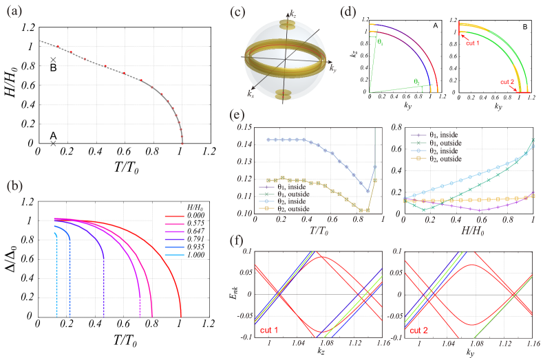
Figure 1: (a) $H-T$ phase diagram. The temperature $T$ is normalized by the zero-field transition temperature $T_{0}$, and the Zeeman field $H$ is normalized by the critical field $H_{0}=0.0138$, the value at the lowest calculated temperature $T_{\rm min}=0.001$. The grey line serves as a guide to the eye. The dashed line indicates a first-order transition. (b) the gap amplitude as a function of the temperature for several different fields, normalized by its value $\Delta_{0}\simeq 0.084$ at $T=T_{\rm min}$ under zero field. The dashed lines mean the discontinuity associated with a first-order transition. (c) 3D cartoon of gap structure. (d) the first quadrant of the $k_{x}=0$ cut plane of the FSs at points A and B in (a). The green lines in B correspond to the FSs in the normal state and the gold-colored lines to the BFSs in the superconducting state. The normal-state FS in A is depicted using the $j_{z}$ decomposition, where the $j_{z}=3/2$ (1/2) component is represented in blue (red). (e) $\theta_{1,2}$ as a function of temperature $T$ and Zeeman field $H$. (f) the quasiparticle dispersion $E_{n{\textbf{k}}}$ along cut 1 and cut 2 in (d)B. The green, blue and red lines correspond to the normal state at $H=0$, and the normal and superconducting states at high fields, respectively.

Formulation— As a simple model exhibiting a BFS, we consider the spherical $j=3/2$ model introduced by Agterberg et al. [1, 2, 45, 46], to elucidate the evolution and instability of the BFS under the Zeeman field. The Hamiltonian is given by

$$\mathcal{H} =\sum_{\textbf{k}}\psi_{\textbf{k}}^{\dagger}\left[(\alpha\textbf{k}^{2}-\mu)\hat{1}+\beta(\textbf{k}\cdot\hat{\textbf{J}})^{2}-g\mu_{B}\hat{J}_{z}H\right]\psi_{\textbf{k}}$$

$$+\sum_{\textbf{k}}\left(\psi_{\textbf{k}}^{\dagger}\hat{\Delta}_{\textbf{k}}\psi_{-\textbf{k}}^{{\dagger}T}+{\rm H.c.}\right),$$ (1)

where $\psi_{\textbf{k}}=(c_{\textbf{k},\frac{3}{2}},c_{\textbf{k},\frac{1}{2}},c_{\textbf{k},-\frac{1}{2}},c_{\textbf{k},-\frac{3}{2}})^{T}$ is the spin-$3/2$ spinor consisting of electron annihilation operators $c_{\textbf{k},j_{z}}$ with wave vector k and the $z$ component of angular momentum $j_{z}$. $\hat{\Delta}_{\textbf{k}}$ denotes the $4\times 4$ matrix of superconducting gap functions, $\hat{\textbf{J}}$ the angular momentum matrix for $j=3/2$, and $\hat{1}$ the $4\times 4$ identity matrix. $\alpha$, which gives the energy scale of the system, is set to $1$ hereafter. $\beta$ and $H$ are the symmetric spin-orbit coupling and the Zeeman field parallel to the $z$ axis, respectively. The $g$ factor and the Bohr’s magneton $\mu_{B}$ are taken as $1$ unless otherwise noted. Electron filling is determined so that $\mu=1$ at $T=0$. Through the Bogoliubov transformation, the Hamiltonian is diagonalized as follows,

$$\mathcal{H}=\sum_{\textbf{k}n}E_{\textbf{k}n}\alpha^{\dagger}_{\textbf{k}n}\alpha_{\textbf{k}n},$$ (2)

where $\alpha_{\textbf{k}n}$ is the annihilation operator of a Bogoliubov quasiparticle (bogolon) and $E_{\textbf{k}n}$ is the excitation energy of the bogolon. Here, we consider an on-site pairing interaction $V_{0}$ and focus on the following local quintet state with TRSB [1, 2, 3],

$$\hat{\Delta}_{\textbf{k}}=\Delta\,(\hat{\eta}_{xz}+i\,\hat{\eta}_{yz})\equiv\Delta\,\hat{\eta}_{+},$$ (3)

where $\hat{\eta}_{xz}=(\hat{J}_{x}\hat{J}_{z}+\hat{J}_{z}\hat{J}_{x})\hat{U}_{T}$, $\hat{\eta}_{yz}=(\hat{J}_{y}\hat{J}_{z}+\hat{J}_{z}\hat{J}_{y})\hat{U}_{T}$, and $\hat{U}_{T}$ is an antisymmetric matrix corresponding to the time-reversal operation multiplied by the complex conjugate. This local quintet pairing state with TRSB induces the chiral $d$-wave pair amplitude [45], giving rise to point nodes along the $k_{z}$-axis and line nodes on the $k_{z}=0$ plane. Additionally, the spontaneously induced magnetic field expands these nodes, forming BFSs [1, 2, 3]. The gap amplitude $\Delta$ is determined by solving the following BCS gap equation,

$$\Delta={V_{0}\over 8}{1\over 4\pi}\!\int\!d\Omega\int_{k_{F}-\delta k}^{k_{F}+\delta k}k^{2}dk\,\Tr[\hat{\eta}_{+}^{\dagger}\expectationvalue{\psi_{-\textbf{k}}\psi_{\textbf{k}}^{T}}]$$ (4)

The integration over $k$ is performed with a step size of $1/50000$ within $\delta k=0.06$ around the Fermi wavenumber $k_{F}$ at each band. The integration for the polar angles is computed numerically using $2500$ meshes, while the azimuthal angles are treated analytically. Hereafter, we set $\beta=-0.1$ and $V_{0}=2.16$, in which a TRSB pairing state with BFSs is expected to emerge [2]. In our case, a local TRSB quintet state with BFSs [Eq.(3)] is obtained below the transition temperature $T_{0}\simeq 0.0088$. In the following, we study the general behavior of the BFS under the Zeeman field based on this case.

Phase diagram and discontinuous transition— First, we consider the $H-T$ phase diagram in Fig. 1(a) and the temperature dependence of the gap amplitude $\Delta$ in Fig. 1(b). At zero field, the temperature dependence of $\Delta$ shows conventional BCS-like behavior. Under finite fields, $\Delta$ shows little variation in the limit of $T\to 0$, and exhibits a discontinuity at high fields $H/H_{0}\gtrsim 0.65$, indicative of the first-order transition. This behavior is summarized in the $H-T$ phase diagram shown in Fig. 1(a). The red points denote superconducting transition points obtained from the gap equation Eq. (4). The grey line serves as a guide to the eye. The dashed line indicates a first-order transition, while the solid line represents a second-order transition. This behavior is consistent with previous studies based on the Ginzburg-Landau theory [47, 48, 49].

Evolution of BFS— Next, we discuss the evolution of BFSs under the Zeeman field, which is not symmetry-protected. Figure 1(c) illustrates the 3D cartoon of BFSs at zero field. The transparent spheres are two normal-state FSs in our model. The red points and lines represent the symmetry-protected point and line nodes expected from Eq. (3). The gold-colored surface is the actual nodal structure obtained from $E_{\textbf{k}n}$. This planar nodal structure corresponds to the BFS. The BFSs near the $k_{z}$ axis are inflated point nodes, while those near the $k_{z}=0$ plane are inflated horizontal line nodes, forming a torus-shaped surface. Figure 1(d) is the first quadrant of the $k_{x}=0$ cross-section of the FSs at points A and B in Fig. 1(a). The green lines represent the FS in the normal state, and the gold-colored lines represent the BFSs in the superconducting state. The 3D structure of the BFSs can be easily inferred from the mirror symmetry of the $k_{z}=0$ plane and the axial symmetry around the $k_{z}$ axis.

In order to quantify the evolution of BFSs, we define the size of the BFSs near $k_{z}$ axis and the $k_{z}=0$ plane as $\theta_{1}$ and $\theta_{2}$, respectively, as indicated in Fig. 1(d)A. The left and right panels of Fig. 1(e) depict the temperature and field dependence of $\theta_{1,2}$, respectively. The left and right panels of Fig. 1(f) represent the quasiparticle dispersions $E_{\textbf{k}n}$ along cuts $1$ and $2$ shown in Fig. 1(d)B, respectively. In the left panel of Fig. 1(e), $\theta_{1}$ and $\theta_{2}$ exhibit nearly identical temperature dependence. This is due to the complete matching of the normal-state dispersions near the point nodes and line nodes. [See green lines in Fig. 1(f)]. Around $T_{0}$ in the left panel of Fig. 1(e), $\theta_{1,2}$ shows a sharp increase due to the small gap amplitude, but except near $T_{0}$, $\theta_{1,2}$ increases monotonically as the temperature decreases, accompanied by the growth of the gap amplitude. This is consistent with the fact that BFSs are induced by spontaneous magnetization. In contrast, the field dependence of $\theta_{1,2}$ differs significantly from the temperature dependence. Compared to the inner $\theta_{1}$ and outer $\theta_{2}$, the outer $\theta_{1}$ and inner $\theta_{2}$ increase almost linearly with the Zeeman field. The BFSs at high field are more clearly seen in Fig. 1(d)B, where the outer BFS near the $k_{z}$ axis and the inner BFS near the $k_{z}=0$ plane expand significantly. This behavior is related to the magnitude of the $j_{z}$ component in the quasiparticle band. The blue lines in Fig. 1(f) show the normal-state quasiparticle band structure at high fields. It can be seen that the large BFS corresponds to a large energy separation at high field, indicating the dominance of $j_{z}=\pm 3/2$ components. Indeed, this can be confirmed by examining the $j_{z}$-resolved normal-state FS in Fig. 1(d)A. Generally, FSs with large spin splitting under the Zeeman field give rise to large BFSs. This evolution of BFSs under external fields can be observed using angle-resolved photoemission spectroscopy (ARPES).

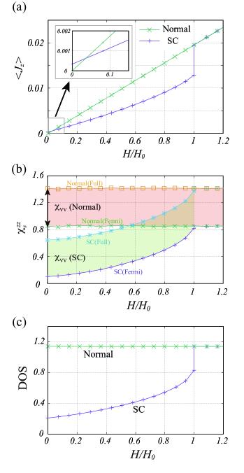
Figure 2: (a) Magnetization, (b) spin susceptibility, and (c) DOS at the Fermi level as a function of Zeeman field at $T=T_{\rm min}$.

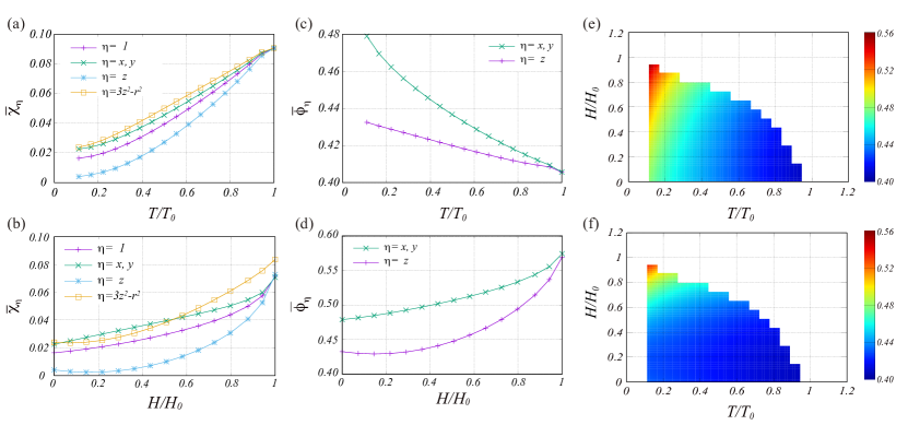
Figure 3: Bogolon correlations $\bar{\chi}_{\eta}$ as a function of (a) temperature at $H=0$ and (b) Zeeman field at $T=T_{\rm min}$. Bogolon pair correlations $\bar{\phi}_{\eta}$ as a function of (c) temperature at $H=0$ and (d) Zeeman field at $T=T_{\rm min}$. The contour map of (e) $\bar{\phi}_{x/y}$ and (f) $\bar{\phi}_{z}$.

Magnetization and spin susceptibility— Figure 2(a) shows magnetization as a function of the Zeeman field at $T=T_{\rm min}$, given by

$$\expectationvalue{J_{z}}=\sum_{\textbf{k}}\sum_{n}\matrixelement{\textbf{k}n}{\hat{J}_{z}}{\textbf{k}n}f(E_{\textbf{k}n}).$$ (5)

In the inset, a small but finite magnetization can be observed even at $H=0$ in the superconducting state, reflecting the TRSB state. Under a finite field, the magnetization increases almost linearly with increasing $H$, reaching approximately $0.67$ times the normal-state value at $H=H_{0}$.

Figure 2(b) depicts the spin susceptibility as a function of the Zeeman field, given by

$$\!\chi_{s}^{zz}=\chi_{\rm Fermi}+\chi_{\rm VV}$$ (6a)

$$\!\chi_{\rm Fermi}=\sum_{\textbf{k}}\sum_{n}|\matrixelement{\textbf{k}n}{{\hat{J}_{z}}}{\textbf{k}n}|^{2}\left(-{\partial f(E_{kn})\over\partial E_{kn}}\right)$$ (6b)

$$\!\chi_{\rm VV}=\sum_{\textbf{k}}\sum_{n\neq n^{\prime}}|\matrixelement{\textbf{k}n}{{\hat{J}_{z}}}{\textbf{k}n^{\prime}}|^{2}\,{f(E_{kn^{\prime}})-f(E_{kn})\over E_{kn}-E_{kn^{\prime}}}$$ (6c)

Here, $\chi_{\rm Fermi}$ represents the FS term, and $\chi_{\rm VV}$ represents the Fermi sea term, that is the Van Vleck term. At zero field, the spin susceptibility $\chi_{s}^{zz}$ decreases to about half of its normal-state value, with most of the residual susceptibility coming from the Van Vleck term $\chi_{\rm VV}$. Under a finite field, $\chi_{\rm VV}$ remains almost unchanged, while $\chi_{\rm Fermi}$ increases rapidly, recovering nearly $96\%$ of the normal-state value at $H_{c}$. The increase in $\chi_{\rm Fermi}$ under the Zeeman field is much larger than what would be expected from the increase in the density of states (DOS) shown in Fig. 2(c), which can be attributed to changes in the wave function induced by the Zeeman field.

Bogolon correlations— The presence of residual DOS or BFS suggests the possibility of further instabilities in the superconducting phase, such as bogolon density wave states or bogolon pairing states, both of which have been studied at zero field thus far [41, 42, 43, 44]. Here, we investigate BFS instability in the $H-T$ phase diagram. First, we consider density-wave-type states, defined by

$$\mathcal{D}_{\eta}(\textbf{q})=\sum_{\textbf{k}}\sum_{n}g_{\eta}(\textbf{k})\alpha_{\textbf{k+q}n}^{\dagger}\alpha_{\textbf{k}n},$$ (7)

where $g_{\eta}(\textbf{k})$ is a form factor, and for simplicity, we consider the spherical harmonics up to second order. Since the FS of the current model does not have a characteristic nesting property, the correlation function at $q=0$ is expected to be large as in ordinary 3D free fermion systems. So, we focus on the $q=0$ correlation, given by

$$\bar{\chi}_{\eta}=\sum_{\textbf{k}}\sum_{n}|g_{\eta}(\textbf{k})|^{2}\left(-\frac{\partial f(E_{\textbf{k}n})}{\partial E_{\textbf{k}n}}\right).$$ (8)

Figure 3(a) displays the temperature dependence of these correlations, which decrease monotonically as the temperature decreases, regardless of the form factor. This behavior results from the reduction in the DOS at the Fermi level due to the opening of the superconducting gap. As depicted in Fig. 3(b), the magnitude of the correlations recovers with the application of the Zeeman field but does not exceed that of the normal state. This suggests that the Pomeranchuk transition of bogolon is unlikely to occur unless the system exhibits a strong nesting property.

Next, let us consider the correlation function of the lowest-order bogolon pair, defined by

$$\bar{\phi}_{\eta}=\sum_{\textbf{k}}\sum_{n}|g_{\eta}(\textbf{k})|^{2}\left(\frac{1-2f(E_{\textbf{k}n})}{2E_{\textbf{k}n}}\right).$$ (9)

Figures 3(c) and 3(d) illustrate the temperature and field dependence, respectively. Unlike the density-wave-type correlation functions, the bogolon pair correlation shows a logarithmic-like increase as the temperature decreases due to the presence of BFS, indicating a potential transition into bogolon pairing states. The correlation for $p_{x}/p_{y}$-wave state is predominant, while the $p_{z}$ pair correlation is relatively enhanced at high fields but remains smaller than the $p_{x}/p_{y}$ pair correlations. In the present case, $p_{x}$ degenerates with $p_{y}$, and according to the BCS weak-coupling theory, a chiral $p_{x}+ip_{y}$ bogolon pairing state is expected to emerge at low temperatures with moderate interactions. Figures 3(e) and 3(f), which show contour maps of the correlation functions, correspond to the phase diagram for bogolon pairing states. In the $p_{x}+ip_{y}$ bogolon pairing state, the torus-shaped BFS near the $k_{z}=0$ plane is gapped, while the BFS near the $k_{z}$ axis remains intact. If the DOS on the torus-shaped BFS is relatively small, a transition from the $p_{x}+ip_{y}$ state to the $p_{z}$-wave state could potentially occur near the critical field at low temperatures. In these bogolon pairing states, the hybridization of pairs with different symmetries, such as the $p$-wave and $d$-wave states, leads to spontaneous inversion symmetry breaking. Thus, the additional transition observed at low temperatures and high fields, involving spontaneous inversion symmetry breaking, could provide supporting evidence for the existence of the BFS state.

Conclusion— In this paper, we have theoretically investigated the evolution and instability of BFS in the spherical $j=3/2$ model under the Zeeman field. Although our findings are based on specific model parameters, they are expected to capture the general qualitative behavor of BFS. The application of the Zeeman field leads to significant growth of the BFS, particularly for those with a large weight of the $j_{z}=\pm 3/2$ component. The evolution of the BFS under the Zeeman field can be observed by spectroscopic methods such as ARPES. From our calculations of bogolon correlation functions, if an additional phase transition occurs in the superconducting phase, it is likely to be a chiral $p$-wave bogolon pairing state rather than a density-wave-type state. This chiral $p$-wave bogolon pairing state, coexisting with the chiral $d$-wave superconducting state, involves spontaneous inversion symmetry breaking. In this state, the torus-shaped BFS near the $k_{z}=0$ plane is gapped, while the BFS near the $k_{z}$ axis remains intact. Investigating the effects of magnetic fields on materials with BFS presents an interesting challenge for future research.

Acknowledgments— We are grateful to S. Hoshino and T. Miki for their useful comments. This work was supported by KAKENHI Grants No. 19H01842, No. 19H05825, and JST SPRING, No. JPMJSP2101.

References

- [1] D. F. Agterberg, P. M. R. Brydon, and C. Timm, Phys. Rev. Lett. 118, 127001 (2017).
- [2] P. M. R. Brydon, D. F. Agterberg, H. Menke, and C. Timm, Phys. Rev. B 98, (2018) 224509.
- [3] H. Menke, C. Timm, and P. M. R. Brydon, Phys. Rev. B 100, 224505 (2019).
- [4] S. Kobayashi, A. Bhattacharya, C. Timm, and P. M. R. Brydon, Phys. Rev. B 105, 134507 (2022).
- [5] A. Bhattacharya and C. Timm, Phys. Rev. B 107, L220501 (2023).
- [6] J. W. F. Venderbos, L. Savary, J. Ruhman, P. A. Lee, and L. Fu, Phys. Rev. X 8, 011029 (2018).
- [7] S. Autti, J. T. Mäkinen, J. Rysti, G. E. Volovik, V. V. Zavjalov, and V. B. Eltsov, Phys. Rev. Research 2, 033013 (2020).
- [8] J. M. Link, I. Boettcher, and I. F. Herbut, Phys. Rev. B 101, 184503 (2020).
- [9] C. Timm and A. Bhattacharya, Phys. Rev. B 104, 094529 (2021).
- [10] Y.-F. Jiang, H. Yao, and F. Yang, Phys. Rev. Lett. 127, 187003 (2021).
- [11] T. Kitamura, S. Kanasugi, M. Chazono, and Y. Yanase, Phys. Rev. B 107, 214513 (2023).
- [12] A. C. Yuan, E. Berg, and S. A. Kivelson, Phys. Rev. B 108, 014502 (2023).
- [13] S. Sumita, T. Nomoto, K. Shiozaki, and Y. Yanase, Phys. Rev. B 99, 134513 (2019).
- [14] Z. Wu and Y. Wang, Phys. Rev. B 108, 224503 (2023).
- [15] S. S. Babkin, A. P. Higginbotham, and M. Serbyn, SciPost Phys. 16, 115 (2024) .
- [16] E. A. Schuberth, B. Strickler, and K. Andres, Phys. Rev. Lett. 68, 117 (1992).
- [17] G. M. Luke, A. Keren, L. P. Le, W. D. Wu, Y. J. Uemura, D. A. Bonn, L. Taillefer, and J. D. Garrett, Phys. Rev. Lett. 71, 1466 (1993).
- [18] E. R. Schemm, W. J. Gannon, C. M. Wishne, W. P. Halperin, and A. Kapitulnik, Science 345, 190 (2014).
- [19] E. R. Schemm, R. E. Baumbach, P. H. Tobash, F. Ron- ning, E. D. Bauer, and A. Kapitulnik, Phys. Rev. B 91, 140506 (2015).
- [20] G. M. Luke, Y. Fudamoto, K. M. Kojima, M. I. Larkin, J. Merrin, B. Nachumi, Y. J. Uemura, Y. Maeno, Z. Q. Mao, Y. Mori, H. Nakamura, and M. Sigrist, Nature 394, 558 (1998).
- [21] J. Xia, Y. Maeno, P. T. Beyersdorf, M. M. Fejer, and A. Kapitulnik, Phys. Rev. Lett. 97, 167002 (2006).
- [22] S. Kittaka, S. Nakamura, T. Sakakibara, N. Kikugawa, T. Terashima, S. Uji, D. A. Sokolov, A. P. Mackenzie, K. Irie, Y. Tsutsumi, K. Suzuki, and K. Machida, Journal of the Physical Society of Japan 87, 093703 (2018).
- [23] H. G. Suh, H. Menke, P. M. R. Brydon, C. Timm, A. Ramires, and D. F. Agterberg, Phys. Rev. Res. 2, 032023(2020).
- [24] Y. Sato, S. Kasahara, T. Taniguchi, X. Xing, Y. Kasahara, Y. Tokiwa, Y. Yamakawa, H. Kontani, T. Shibauchi, and Y. Matsuda, Proceedings of the National Academy of Sciences 115, 1227 (2018).
- [25] T. Hanaguri, K. Iwaya, Y. Kohsaka, T. Machida, T. Watashige, S. Kasahara, T. Shibauchi, and Y. Matsuda, Science Advances 4, eaar6419 (2018).
- [26] Z. Yu, K. Nakamura, K. Inomata, X. Shen, T. Mikuri, K. Matsuura, Y. Mizukami, S. Kasahara, Y. Matsuda, T. Shibauchi, Y. Uwatoko, and N. Fujiwara, Communications Physics 6, 175 (2023).
- [27] K. Matsuura, M. Roppongi, M. Qiu, Q. Sheng, Y. Cai, K. Yamakawa, Z. Guguchia, R. P. Day, K. M. Kojima, A. Damascelli, Y. Sugimura, M. Saito, T. Takenaka, K. Ishihara, Y. Mizukami, K. Hashimoto, Y. Gu, S. Guo, L. Fu, Z. Zhang, F. Ning, G. Zhao, G. Dai, C. Jin, J. W. Beare, G. M. Luke, Y. J. Uemura, and T. Shibauchi, Proceedings of the National Academy of Sciences 120, e2208276120 (2023).
- [28] T. Nagashima, T. Hashimoto, S. Najafzadeh, S. Ouchi, T. Suzuki, A. Fukushima, S. Kasahara, K. Matsuura, M. Qiu, Y. Mizukami, K. Hashimoto, Y. Matsuda, T. Shibauchi, S. Shin, and K. Okazaki, Research Square report, Research Square, https://doi.org/10.21203/rs.3.rs-2224728/v1.
- [29] C. Setty, S. Bhattacharyya, Y. Cao, A. Kreisel, and P. J. Hirschfeld, Nature Communications 11, 523 (2020).
- [30] C. Setty, Y. Cao, A. Kreisel, S. Bhattacharyya, and P. J. Hirschfeld, Phys. Rev. B 102, 064504 (2020).
- [31] Y. Cao, C. Setty, L. Fanfarillo, A. Kreisel, and P. J. Hirschfeld, Phys. Rev. B 108, 224506 (2023).
- [32] K. R. Islam and A. Chubukov, npj Quantum Materials 9, 28 (2024).
- [33] Y. Cao, C. Setty, A. Kreisel, L. Fanfarillo, and P. J. Hirschfeld, Phys. Rev. B 110, L020503 (2024).
- [34] C. J. Lapp, G. Börner, and C. Timm, Phys. Rev. B 101, 024505 (2020).
- [35] H. Oh, D. F. Agterberg, and E.-G. Moon, Phys. Rev. Lett. 127, 257002 (2021).
- [36] T. Miki, S.-T. Tamura, S. Iimura, and S. Hoshino, Phys. Rev. B 104, 094518 (2021).
- [37] T. Miki, H. Ikeda, and S. Hoshino, Phys. Rev. B 109, 094502 (2024).
- [38] D. Kim, S. Kobayashi, and Y. Asano, Journal of the Physical Society of Japan 90, 104708 (2021).
- [39] J. Ahn and N. Nagaosa, Nature Communications 12, 1617 (2021).
- [40] R. Ohashi, S. Kobayashi, S. Kanazawa, Y. Tanaka, and Y. Kawaguchi, Phys. Rev. B 110, 104515 (2024).
- [41] S.-T. Tamura, S. Iimura, and S. Hoshino, Phys. Rev. B 102, 024505 (2020).
- [42] H. Oh and E.-G. Moon, Phys. Rev. B 102, 020501 (2020).
- [43] C. Timm, P. M. R. Brydon, and D. F. Agterberg, Phys. Rev. B 103, 024521 (2021).
- [44] I. F. Herbut and J. M. Link, Phys. Rev. B 103, 144517 (2021).
- [45] P. M. R. Brydon, L. Wang, M. Weinert, and D. F. Agterberg, Phys. Rev. Lett. 116, 177001 (2016).
- [46] J. M. Luttinger, and W. Kohn, Phys. Rev. 97, 869 (1955).
- [47] G. Sarma, Journal of Physics and Chemistry of Solids 24, 1029 (1963).
- [48] K. Maki and T. Tsuneto, Pauli Paramagnetism and Superconducting State, Progress of Theoretical Physics 31, 945 (1964).
- [49] T. Sato, S. Kobayashi, and Y. Asano, arXiv:2308.02211.