KA-GNN: Kolmogorov-Arnold Graph Neural Networks for Molecular Property Prediction

Abstract

Molecular property prediction is a crucial task in the process of Artificial Intelligence-Driven Drug Discovery (AIDD). The challenge of developing models that surpass traditional non-neural network methods continues to be a vibrant area of research. This paper presents a novel graph neural network model—the Kolmogorov-Arnold Network (KAN)-based Graph Neural Network (KA-GNN), which incorporates Fourier series, specifically designed for molecular property prediction. This model maintains the high interpretability characteristic of KAN methods while being extremely efficient in computational resource usage, making it an ideal choice for deployment in resource-constrained environments. Tested and validated on seven public datasets, KA-GNN has shown significant improvements in property predictions over the existing state-of-the-art (SOTA) benchmarks.

1 Introduction

Drug development is a complex and costly process, typically requiring decades of time and substantial investment [1, 2, 3]. In this challenging landscape, artificial intelligence (AI) has become particularly valuable, significantly impacting the prediction of molecular properties and showing immense promise in drug design [4, 5]. AI has greatly advanced virtual screening processes, potentially reducing the time and investment required [6, 7]. However, developing effective molecular representations and features remains a complex challenge. AI-based molecular models, which drive these advancements, generally fall into two categories: those based on molecular descriptors and end-to-end deep learning models [8].

The first category relies on molecular descriptors or fingerprints as input features for machine learning algorithms. This process, known as featurization or feature engineering, involves not only capturing physical, chemical, and biological properties but also incorporating a wide array of fingerprints based on molecular structure information. Among these, structure-based fingerprints, particularly those derived from topological data analysis methods, have proven highly effective in molecular representation and featurization [9, 10, 11, 12]. The integration of these fingerprints with learning models has achieved significant success in various stages of drug design, including protein-ligand binding affinity prediction [13, 14, 15], protein mutation analysis [16, 17], and drug discovery [18], among other areas.

The second category encompasses end-to-end deep learning models, where molecules are represented using Simplified Molecular Input Line Entry System (SMILES) strings, images, or molecular graphs, and various deep learning architectures such as Transformers, Convolutional Neural Networks (CNNs), and Graph Neural Networks (GNNs) are employed for molecular property prediction [19, 20, 21, 22]. Among these, molecular graphs, particularly those based on covalent bonds, are the most common representations of molecular topology at the atomic level. Numerous geometric deep learning models have been developed based on these molecular graphs, including Graph Convolutional Networks (GCNs) [23], graph autoencoders [24], and graph transformers [25]. These models are widely used in molecular data analysis and drug design. Additionally, molecular descriptors based on non-covalent interactions have recently demonstrated strong performance in predicting protein-ligand and protein-protein binding affinities [26, 12]. This suggests that new geometry-based molecular graph representations could potentially outperform traditional covalent-bond-based graphs. Integrating these geometry-based molecular graphs into geometric deep learning (GDL) models could enhance model performance and provide a better understanding of molecular geometry [27].

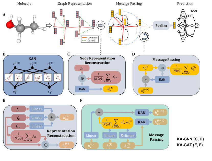
Figure 1: Overview of the KA-GNN model. A. Flowchart of the KA-GNN model. B. Example of a KAN at layer $l$ using Fourier series functions as pre-activation functions, illustrated for a case with 2 input dimensions and 3 output dimensions. C. Architecture for reconstructing node features used in the message-passing process of the GNN. D. Architecture of message passing in the KA-GNN at layer $l$.

Based on the Kolmogorov-Arnold representation theorem, Kolmogorov-Arnold Networks (KANs) have recently been proposed as a promising alternative to Multi-layer Perceptrons (MLPs) [28]. Due to their unique architecture and potential advantages, KANs stand out in several aspects. While MLPs, inspired by the universal approximation theorem, use fixed activation functions on nodes, KANs, inspired by the Kolmogorov-Arnold representation theorem, place learnable activation functions on edges, resulting in a fully-connected structure without linear weight matrices. This innovative design allows KANs to achieve higher accuracy and parameter efficiency compared to MLPs, particularly in solving partial differential equations. Recent research has explored various applications of KAN across different domains. Bozorgasl et al. [29] enhanced KAN by incorporating wavelet functions to improve interpretability and performance in capturing both high and low-frequency data components. Genet et al. [30] combined KANs with LSTMs, improving multi-step time series forecasting accuracy and efficiency. Cheon et al. [31] integrated KAN with pre-trained CNN models for remote sensing scene classification, demonstrating its effectiveness in this field.

In this paper, we present the development of KA-GNN, a novel model for molecular property prediction for the first time. The architecture of KA-GNN is shown in Figure 1. Our KA-GNN model leverages Fourier series and incorporates the Kolmogorov-Arnold Network (KAN) architecture to enhance the performance of a Graph Neural Network (GNN). In fact, our approach applies KAN to various components of the GNN, including node feature initialization, the message passing process, and graph classification tasks. A notable modification is the adjustment of the pre-activation function in KAN from B-splines to Fourier basis functions. Furthermore, our model considers both covalent bonds and non-covalent interactions defined by a cut-off distance, to construct the molecular graph representation in the GNN. These innovative adjustments ensure that KA-GNN remains parameter-efficient, while experimental results demonstrate that our model surpasses existing state-of-the-art pre-trained models across several benchmark tests. This highlights KA-GNN’s significant potential in drug development and molecular property prediction.

2 Related Work

In this section, we review the related research concerning molecular representation and then detail recent advances in graph neural networks for property prediction.

2.1 Kolmogorov-Arnold Network

Inspired by the Kolmogorov-Arnold representation theorem, Liu et al. [28] introduced the Kolmogorov-Arnold Network (KAN), a novel deep learning architecture that serves as a promising alternative to the traditional Multi-Layer Perceptron (MLP). Compared to MLP, KAN exhibits enhanced expressive power, parameter efficiency, high interpretability, and wide applicability.

Recent research has explored various applications of KAN in different domains. For instance, Bozorgasl et al. [29] incorporated wavelet functions into the Kolmogorov-Arnold network framework to improve interpretability and performance in capturing both high-frequency and low-frequency components of input data. Genet et al. [30] combined the strengths of KANs and LSTMs to enhance the accuracy and efficiency of multi-step time series forecasting. Additionally, Cheon et al. [31] integrated KAN with various pre-trained CNN models for remote sensing scene classification, demonstrating its efficacy in this domain.

These studies illustrate the versatility and potential of KAN in addressing diverse challenges across different fields, further validating its role as a robust and efficient deep learning architecture.

2.2 Molecular representation

Learning molecular representations is crucial for predicting the properties of compounds. At present, the modeling methods for molecular representations mainly fall into the following categories: sequence-based methods, graph-based methods and mixed data-based methods, [32, 33, 34]. Sequence-based methods[35, 36, 37] involve the use of sequences, such as SMILES strings, to represent molecules. These sequences are then processed using techniques inspired by natural language processing (NLP), taking advantage of the sequential nature of the data. However, the deep learning models are hindered by the nonunique nature of the SMILES string [36]. Graph-based methods consider molecules as graphs where atoms are nodes and bonds are edges. This category utilizes graph neural networks (GNNs) to capture the topological structure of molecules, making it highly effective for studying molecular connectivity and properties [38, 39, 40, 41]. AGBT[42] combined the SMILES string and a structure graph to construct molecular representation. DGL-LifeSci[43] integrated seven graph based models for molecular property prediction and pretrained models.

2.3 Graph Neural Network for Molecular Property Prediction

Graph neural network models have played a pivotal role in molecular data analysis. Traditional GNN models represent molecules as the defactor covalent-bond-based molecular graphs, and use major GNN architectures to learn molecular properties [44, 45, 46, 47]. With the importance of non-covalent bonds, cutoff-distance-based molecular graph representations have been widely employed in GNN models, such as DimeNet [48], Mol-GDL [27], etc. Further, higher-order interactions (beyond pair-wise forces) has been explicitly incorporated into GNN models, including ALIGNN [46], GEM [47], GemNet [49], etc, by the consideration of bond angles, dihedral angles, torsion angles, and other local geometric information. In particular, these higher-order terms can be directly related to MD force field information [50]. Finally, pre-training process has been adopted to further improve the accuracy of GNN models, such as N-Gram [51], PretrainGNN [52], GraphMVP[53], GEM [47], MolCLR [54], Uni-mol[55], SMPT[56], etc.

3 Method

3.1 Kolmogorov-Arnold representation theorem

The Kolmogorov–Arnold Representation Theorem (or Superposition Theorem) is a milestone in the field of real analysis and approximation theory. It states that every multivariate continuous function can be represented as superposition of the addition of continuous functions of one variable. This theorem not only solves Hilbert’s thirteenth problem itself but also generalizes it to a broader form.

Vladimir Arnold and Andrey Kolmogorov’s works [57] prove that arbitrary multivariate continuous function $f$ can be written as a finite composition of continuous functions of a single variable and the binary operation of addition. More specifically,

$$f(x_{1},\ldots,x_{n})=\sum_{q=0}^{2n+1}\Phi_{q}\left(\sum_{p=1}^{n}\phi_{q,p}(x_{p})\right),$$ (1)

where $n$ denote the number of variables of the function $f$. $\Phi_{q}:\mathbb{R}\to\mathbb{R}$ and $\phi_{q,p}:[0,1]\to\mathbb{R}$ are continues function.

3.2 Kolmogorov-Arnold Network (KAN)

Inspired by the Kolmogorov-Arnold representation theorem, Liu et al. [28] proposed a new deep learning architecture called the Kolmogorov-Arnold Network (KAN) as a promising alternative to the Multi-Layer Perceptron (MLP). To enhance the KAN’s representational capacity and leverage modern techniques (e.g., backpropagation) for training the networks, KAN transcends several limitations of the Kolmogorov-Arnold representation theorem:

• KAN does not adhere to the original depth-2 width-$(2n+1)$ representation; instead, it generalizes to arbitrary widths and depths. Specifically, let the activation values in layer $l$ be denoted by $\mathbf{x}^{(l)}:=(x_{1}^{(l)},x_{2}^{(l)},\cdots,x_{n_{l}}^{(l)})$, where $n_{l}$ is the width of layer $l$. The activation value in layer $l+1$ is then simply the sum of all incoming post-activations:

  $$x_{j}^{(l+1)}=\sum_{i=1}^{n_{l}}\phi_{j,i}^{(l)}(x_{i}^{(l)}),\quad j=1,\ldots,n_{l+1}.$$ (2)

  Here, $\phi_{j,i}^{(l)}$ for $i=1,\ldots,n_{l}$ and $j=1,\ldots,n_{l+1}$ are the pre-activation functions in layer $l$. The roles of these functions in KAN are analogous to the roles of the inner functions $\phi_{q,p}$ in equation 1.

• Although many constructive proofs of the Kolmogorov-Arnold representation theorem indicate that the inner functions $\phi_{q,p}$ in equation 1 are highly non-smooth [58, 59, 60], KAN opts for smooth functions as pre-activation functions $\phi_{j,i}^{(l)}$ to facilitate backpropagation. Liu et al. [28] selected functions based on B-splines. In this paper, we consider Fourier series functions.

Features Type		Description	Type	Size
Atom	CGCNN	Atomic number, Radius, and electronegativity	One-Hot	92
Covalent Bond	Bond Directionality	None, Beginwedge, Begindash, etc.	One-Hot	7
	Bond Type	Single, Double, Triple, or Aromatic.	One-Hot	4
	Bond Length	Numerical and square length of the bond.	Float	2
	In Ring	Indicates if the bond is part of a chemical ring.	One-Hot	2
Cutoff Bond	Atom charges	Atoms charges in Molecular ($q_{i}$, $q_{j}$, $q_{i}$$\cdot$ $q_{j}$)	Float	3
	Distance between atoms	Distance between atoms ($\frac{1}{d_{ij}}$, $\frac{1}{d_{ij}^{6}}$, $\frac{1}{d_{ij}^{12}}$)	Float	3

Table 1: Features Type and Description in KA-GNN model. Here we list both atom, covalent bond, and cuttoff bond features.

3.3 Graph Representation for Molecules

Molecules can naturally be viewed as graph structures, where the nodes represent atoms and the edges represent covalent bonds. Traditional molecular graphs typically include only the covalent bonds between atoms. However, in molecular dynamics, non-covalent interactions between atoms also significantly influence molecular properties. Therefore, when constructing the molecular graph, KA-GNN includes both covalent bonds and non-covalent interactions where atomic distances are less than 5 angstroms. These non-covalent bonds are treated as cut-off edges, providing a comprehensive reflection of the complex interactions within the molecule. The Graph Representation in the Figure 1 A illustrates the complex interactions within the molecule, highlighting both the covalent bonds (solid lines) and non-covalent cut-off bonds (dashed lines) with distances less than 5 angstroms are considered in our KA-GNN model.

The features of the graph are meticulously designed to encapsulate the various atomic properties and interactions detailed in molecular dynamics (MD) force fields. Specifically, our atomic features—comprising atomic number, radius, and electronegativity—are derived using Rdkit, following the approach in CGCNN [61]. Table 1 presents a comprehensive listing of the features for covalent bonds and non-covalent cutoff edges.

3.4 KA-GNN Method

Fourier-based KAN function

To optimize the network and avoid complex calculations, we utilize Fourier series as the pre-activation functions in Equation 2:

$$\phi_{j,i}^{(l)}(x)=\sum_{k=1}^{K}\left(A_{k,j,i}^{(l)}\cos(kx)+B_{k,j,i}^{(l)}\sin(kx)\right),$$ (3)

where $K$ is the number of harmonics, and $A_{k,j,i}^{(l)}$ and $B_{k,j,i}^{(l)}$ are learnable parameters initially sampled from a normal distribution $\text{N}\left(0,\frac{1}{n_{l+1}\times K}\right)$.

Consequently, the activation value at the $j$-th neuron in layer $l+1$ can be obtained by:

$$x_{j}^{(l+1)}=\sum_{i=1}^{n_{l}}\sum_{k=1}^{K}\left(A_{k,j,i}^{(l)}\cos(kx_{i}^{(l)})+B_{k,j,i}^{(l)}\sin(kx_{i}^{(l)})\right),$$ (4)

where $\mathbf{x}^{(l)}=(x_{1}^{(l)},x_{2}^{(l)},\dots,x_{n_{l}}^{(l)})$ denotes the input vector of activation values in layer $l$ of the KAN, and $\mathbf{x}^{(l+1)}=(x_{1}^{(l+1)},x_{2}^{(l+1)},\dots,x_{n_{l+1}}^{(l+1)})$ represents the output vector. Equation 4 can be concisely expressed as: $\mathbf{x}^{(l+1)}=\text{KAN}_{l}(\mathbf{x}^{(l)})$, where $\text{KAN}_{l}(\cdot)$ denotes the above KAN function in layer $l$. This network is integrated into a graph neural network, culminating in a novel architecture named KA-GNN, which is employed for molecular property prediction tasks.

Given that the inner functions in Equation 1 of the Kolmogorov-Arnold representation theorem can exhibit significant non-smoothness, we do not use this theorem as the foundational theory for showing the approximation capability of our model. Instead, we base our approach on the extension of Carleson’s theorem [62] regarding the convergence of Fourier series for multivariable functions, as proved by Fefferman in [63]:

Theorem 1

Let $\mathbf{Z}^{n}$ denote the $n$-dimensional integer lattice, and let $Z_{N}^{n}=\{1,2,\ldots,N\}^{n}\subset\mathbf{Z}^{n}$. Then for the function $f\in L^{2}([0,2\pi]^{n})$ and its Fourier expansion:

$$f(\vec{\mathbf{x}})\sim\sum_{\vec{\mathbf{k}}\in\mathbf{Z}^{n}}\left(a_{\vec{\mathbf{k}}}\cos(\vec{\mathbf{k}}\cdot\vec{\mathbf{x}})+b_{\vec{\mathbf{k}}}\sin(\vec{\mathbf{k}}\cdot\vec{\mathbf{x}})\right),$$

where $x\in[0,2\pi]^{n}\text{ and }L^{2}([0,2\pi]^{n})$ denotes the space of square-integrable functions on $[0,2\pi]^{n}$, which consists of all functions $f$ such that $\int_{[0,2\pi]^{n}}|f(\vec{\mathbf{x}})|^{2}\,d\vec{\mathbf{x}}<\infty$. We have

$$f(\vec{\mathbf{x}})=\lim_{N\to\infty}\sum_{\vec{\mathbf{k}}\in Z_{N}^{n}}\left(a_{\vec{\mathbf{k}}}\cos(\vec{\mathbf{k}}\cdot\vec{\mathbf{x}})+b_{\vec{\mathbf{k}}}\sin(\vec{\mathbf{k}}\cdot\vec{\mathbf{x}})\right)$$

almost everywhere.

The above theorem demonstrates the strong approximation capability of Fourier series, which is why we adopt Fourier series as the foundational basis for our model. Therefore, we retain the architecture of the Kolmogorov-Arnold network but replace the pre-activation functions with Fourier series. We can further prove that this new KAN architecture provides the potential of robust approximation capability:

Theorem 2

Let $f\in L^{2}([0,2\pi]^{n})$ be a square-integrable function. For almost every $\vec{x}\in[0,2\pi]^{n}$ and for any $\epsilon>0$, there exist a positive integer $K$ and a sequence of Fourier-based KAN functions $\mathrm{KAN}_{l}$ at multiple layers $l=0,1,\ldots,L$, such that the number of harmonics in the pre-activation functions of these KAN functions does not exceed $K$, and

$$\left|f(\vec{x})-\mathrm{KAN}_{L}\circ\mathrm{KAN}_{L-1}\circ\cdots\circ\mathrm{KAN}_{0}(\vec{x})\right|<\epsilon,$$

where $\circ$ denotes function composition.

In summary, our model extends the Kolmogorov-Arnold Network (KAN) architecture by incorporating Fourier series as pre-activation functions to enhance approximation capability. By integrating this Fourier-based KAN within a Graph Neural Network (GNN) framework, we achieve a model with good performance and robustness.

The model represents a molecule as a graph $G=(V,E)$, where $V$ denotes the set of nodes (atoms) and $E$ denotes the set of edges, defined as $E=E_{\text{chem}}\cup E_{\text{cutoff}}$. Here, $E_{\text{chem}}$ includes the covalent bonds, while $E_{\text{cutoff}}=\{uv\mid d(u,v)\leq 5\text{\AA}\}$ represents pairs of nodes within a cut-off distance of 5 angstroms. Each node $v\in V$ is associated with a feature vector $f_{v}$, which is a 92-dimensional vector composed of one-hot encoded representations of atomic properties, following the approach described in [61]. Similarly, each edge $uv\in E$ is associated with a feature vector $f_{uv}$, which is a 21-dimensional vector incorporating both chemical and geometrical information of the bond $uv$. Detailed descriptions of the feature vectors are provided in Table 1. The above feature vectors are utilized to reconstruct the initial node features $h_{v}^{(0)},v\in V$ for the graph neural network (GNN) in our model.

KA-GNN Model

the message passing are as following:

$$h_{v}^{(0)}:=\text{KAN}_{\text{ini}}\left(f_{v}\oplus(\frac{1}{|N(v)|}\sum_{u\in N(v)}f_{uv})\right),$$ (5)

where $N(v)$ is the set of neighbors of node $v$ ($v$ is not included), $|N(v)|$ denotes the number of neighbors of $v$, and $\oplus$ denotes the concatenation of vectors. The message passing process in layer $l$ can be expressed as follows:

$$h_{v}^{(l+1)}:=h_{v}^{(l)}+\text{KAN}_{l}\left(h_{v}^{(l)}\oplus(\frac{1}{|N(v)|}\sum_{u\in N(v)}h_{u}^{(l)})\right).$$ (6)

The initial KAN layer, $\text{KAN}_{\text{ini}}$, and the $l$-th KAN layer, $\text{KAN}_{l}$, correspond to the KAN function introduced in Equation 4, with their output dimensions set to 64. The input dimensions of these layers are adapted to fit the respective input vectors.

KA-GAT Model

by combining the characteristics of the attention score the message passing for the KA-GAT as as following:

The Mol-GAT utilized the graph representation features to generate the initial features $h_{v}^{(0)}$ and $h_{uv}^{(0)}$.

$$\begin{split}h_{v}^{(0)}&:=\left(f_{v}\oplus(\frac{1}{|N(v)|}\sum_{u\in N(v)}f_{(u,v)})\right),\\ h_{uv}^{(0)}&:=\text{Linear}\left(f_{v}\right)+\text{Linear}\left(f_{uv}\right)+\text{Linear}\left(f_{u}\right)\end{split}$$ (7)

During the message passing process of the Mol-GAT, we use the initial features to calculate the attention score for the aggregation operation.

$$\begin{split}z_{v}^{(l+1)}&:=\text{Linear}\left(h_{v}^{(l)}\right),z_{u}^{(l+1)}:=\text{Linear}\left(h_{u}^{(l)}\right),\\ \alpha_{uv}&:=\text{Softmax}\left(h_{uv}^{(l)}\right),m_{u}^{(l+1)}:=z_{u}^{(l+1)}\cdot\alpha_{uv}\\ m_{v}^{(l+1)}&:=z_{v}^{(l+1)}+\left(\sum_{u\in N(v)}m_{u}^{(l+1)}\right)\end{split}$$ (8)

Then we use KAN for information updating.

$$h_{v}^{(l+1)}:=\text{KAN}\left(m_{v}^{(l+1)}\right),h_{uv}^{(l+1)}:=\text{KAN}(h_{uv}^{(l)})$$ (9)

Readout

Following the message passing process, we apply average pooling over all node feature vectors to obtain a final representation of the molecular graph $G$. Subsequently, we apply a one-layer or two-layer KAN as a readout function on this representation for the prediction task.

The loss function employed in our model is the cross-entropy loss function, defined as follows:

$$\mathcal{L}=-\sum_{i}\left(y_{i}\log(\hat{y}_{i})+(1-y_{i})\log(1-\hat{y}_{i})\right),$$

where $y_{i}$ denotes the actual label, and $\hat{y}_{i}$ denotes the predicted label. The architecture of the KA-GNN and KA-GAT model is illustrated in Figure 1.

4 Experiments

Table 2: Performance metrics of various models across different datasets, The best performance is indicated as bold and the second-best performance is in bold. Standard deviations are indicated as subscripts.

Model	BACE	BBBP	ClinTox	SIDER	Tox21	HIV	MUV
No. mol	1513	2039	1478	1427	7831	41127	93808
No. avg atoms	65	46	50.58	65	36	46	43
No. tasks	1	1	2	27	12	1	17
D-MPNN	0.809(0.006)	0.710(0.003)	0.906(0.007)	0.570(0.007)	0.759(0.007)	0.771(0.005)	0.786(0.014)
AttentiveFP	0.784(0.022)	0.663(0.018)	0.847(0.003)	0.606(0.032)	0.781(0.005)	0.757(0.014)	0.786(0.015)
N-GramRF	0.779(0.015)	0.697(0.006)	0.775(0.040)	0.668(0.007)	0.743(0.009)	0.772(0.004)	0.769(0.002)
N-GramXGB	0.791(0.013)	0.691(0.008)	0.875(0.027)	0.655(0.007)	0.758(0.009)	0.787(0.004)	0.748(0.002)
PretrainGNN	0.845(0.007)	0.687(0.013)	0.726(0.015)	0.627(0.008)	0.781(0.006)	0.799(0.007)	0.813(0.021)
GROVE_base	0.821(0.007)	0.700(0.001)	0.812(0.030)	0.648(0.006)	0.743(0.001)	0.625(0.009)	0.673(0.018)
GROVE_large	0.810(0.014)	0.695(0.001)	0.762(0.037)	0.654(0.001)	0.735(0.001)	0.682(0.011)	0.673(0.018)
GraphMVP	0.812 (0.009)	0.724 (0.016)	0.791 (0.028)	0.639 (0.012)	0.759 (0.005)	0.770 (0.012)	0.777 (0.006)
MolCLR	0.824 (0.009)	0.722 (0.021)	0.912 (0.035)	0.589 (0.014)	0.750 (0.002)	0.781 (0.005)	0.796 (0.019)
GEM	0.856(0.011)	0.724(0.004)	0.901(0.013)	0.672(0.004)	0.781(0.001)	0.806(0.009)	0.817(0.005)
Mol-GDL	0.863(0.019)	0.728(0.019)	0.966(0.002)	0.831(0.002)	0.794(0.005)	0.808(0.007)	0.675(0.014)
Uni-mol	0.857 (0.002)	0.729 (0.006)	0.919 (0.018)	0.659 (0.013)	0.796 (0.005)	0.808 (0.003)	0.821 (0.013)
SMPT	0.873 (0.015)	0.734 (0.003)	0.927 (0.002)	0.676 (0.050)	0.797 (0.001)	0.812 (0.001)	0.822 (0.008)
KA-GNN	0.890(0.014)	0.787(0.014)	0.989(0.003)	0.842(0.001)	0.799(0.005)	0.821(0.005)	0.834(0.009)
KA-GAT	0.882(0.007)	0.770(0.021)	0.994(0.003)	0.846(0.002)	0.800(0.004)	0.815(0.008)	0.825(0.005)

4.1 Dataset

For an extensive validation of our KA-GNN model, we used seven benchmark datasets from MoleculeNet [64]. Three datasets are from the biophysics domain: MUV, HIV, and BACE. MUV, a subset of PubChem BioAssay refined using nearest neighbor analysis, is designed for validating virtual screening techniques. The HIV dataset measures the ability of molecules to inhibit HIV replication. BACE includes both quantitative (IC50) and qualitative (binary) binding results for inhibitors of human $\beta$-secretase 1 (BACE-1). The remaining four datasets are from the physiology domain: BBBP, Tox21, SIDER, and ClinTox. BBBP contains binary labels for blood-brain barrier penetration. Tox21 provides qualitative toxicity measurements for 12 biological targets. SIDER is a database of marketed drugs and their adverse drug reactions (ADRs), grouped into 27 system organ classes. ClinTox includes qualitative data on FDA-approved drugs and those that failed clinical trials due to toxicity.

The original data in these datasets are SMILES strings of the molecules. During data preprocessing, we use the Merck molecular force field (MMFF94) function from the RDKit package to generate 3D molecular structures from the SMILES strings. Based on the generated structures, we construct graphs for the GNN in our KA-GNN model to predict the relevant properties. For evaluation, we use the Receiver Operating Characteristic - Area Under the Curve (ROC-AUC) metric. Additionally, we employ the scaffold splitting method [65] to divide the datasets into training, validation, and test sets in a ratio of 8:1:1.

4.2 Baselines

Our KA-GNN model has been evaluated alongside a selection of state-of-the-art GNN architectures, including both pre-trained and non-pre-trained models. These encompass MPNN frameworks like D-MPNN [44], attention-driven models such as AttentiveFP [45], and multi-scale approaches exemplified by Mol-GDL [27]. Importantly, our comparisons also extend to geometry-focused graph models that leverage pre-training, including N-Gram [51], PretrainGNN [52], GROVER [25], GraphMVP [66], MolCLR [54], GEM [47], Uni-mol [55], and SMPT [56].

4.3 Setting

In our study, to specifically enhance the model’s performance across various datasets, we selected appropriate hyperparameter settings (such as learning rate, batch size, etc.), details of which can be found in Supplementary Materials. We set the epochs to 1000 and executed the code on a machine equipped with a NVIDIA RTX A5000 32GB GPUs. Each dataset was evaluated five times, calculating the mean as the final metric and recording the standard deviation.

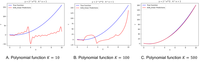
Figure 2: Powerful Fourier KAN fits Polynomial function by adjusting the parameter $K$.

4.4 Results

The comparative results in Table 2 further confirm the superiority of the KA-GNN model. Our model achieves state-of-the-art performance across all benchmark datasets, excelling particularly on complex and challenging datasets such as ClinTox and MUV. These results demonstrate the robust capability of our model in handling molecular data.

We attribute the effectiveness and power of the KA-GNN model to three core innovations:

First, in constructing molecular graphs, we incorporate edges not only from traditional covalent bonds but also from non-covalent interactions based on a cut-off distance. This approach significantly enhances the model’s understanding of molecular structures, enabling it to capture more molecular properties than traditional covalent interactions alone.

Second, we integrate the Kolmogorov-Arnold Network (KAN) into our model. KAN significantly reduces the number of parameters while providing high interpretability and enhanced expressive power, leading to superior performance of the KA-GNN model.

Third, we replace the pre-activation function in the KAN model from the original B-splines to Fourier series functions. Fourier series functions, widely used in signal processing, have proven effective in our model for analyzing and learning high-dimensional graphical data. By learning and optimizing the coefficients of these Fourier series functions for different variables, KA-GNN improves the accuracy and stability of predictions when dealing with complex chemical and biological data structures.

These three innovations collectively contribute to the outstanding performance of KA-GNN, making it a powerful tool for molecular property prediction.

Powerful Fourier KAN

The parameter $K$, representing the number of harmonics, is pivotal in the Fourier KAN model. Increasing $K$ allows the model to include a greater number of Fourier series terms in the approximation, thereby enhancing its capacity to approximate more complex functions. However, increasing $K$ also amplifies computational costs and the risk of overfitting. Conversely, smaller $K$ values mitigate these risks but may compromise the model’s expressiveness. Thus, selecting an optimal $K$ is critical for balancing expressiveness with computational efficiency in the Fourier KAN model. Figure 2 shows the fitting of different $K$ values on Polynomial function. More details for Fourier KAN can been found in Appendix A.4.

Ablation Study

Our model utilizes Fourier-based Kolmogorov-Arnold Network (KAN) as the underlying framework, which is very different from traditional MLP-based GNNs. To evaluate the performance of this GNN architecture in predicting molecular properties, we tested GNN models incorporating MLP, original KAN, and Fourier-based KAN. These models are denoted as GNN(MLP), GNN(KAN), KA-GNN, GAT(MLP), GAT(KAN) and KA-GAT respectively. Table 3 summarizes the results, which clearly demonstrate that the KA-GNN model significantly outperforms both the GNN(MLP) and GNN(KAN) models, delivering superior performance across various benchmark datasets.

Table 3: Comparison of the performance of GNN and GAT models across various datasets.

Dataset	GNN Models			GAT Models
	GNN(MLP)	GNN(KAN)	KA-GNN	GAT(MLP)	GAT(KAN)	KA-GAT
BACE	0.835(0.014)	0.771(0.012)	0.890(0.014)	0.834(0.012)	0.808(0.009)	0.882(0.007)
BBBP	0.735(0.011)	0.723(0.008)	0.787(0.014)	0.707(0.007)	0.657(0.004)	0.770(0.021)
ChinTox	0.979(0.004)	0.973(0.006)	0.989(0.003)	0.983(0.006)	0.948(0.003)	0.994(0.002)
SIDER	0.834(0.001)	0.824(0.003)	0.842(0.001)	0.836(0.002)	0.825(0.004)	0.845(0.002)
Tox21	0.747(0.006)	0.724(0.005)	0.799(0.005)	0.751(0.007)	0.731(0.012)	0.800(0.004)
HIV	0.762(0.005)	0.753(0.007)	0.821(0.005)	0.761(0.003)	0.744(0.018)	0.815(0.008)
MUV	0.741(0.006)	0.638(0.008)	0.834(0.009)	0.784(0.019)	0.792(0.013)	0.825(0.005)

5 Conclusion

The KA-GNN model represents a significant advancement in molecular characterization by leveraging molecular dynamics to construct graphs that incorporate both covalent and non-covalent bonds. Built upon the KAN architecture with Fourier series functions as pre-activation functions, this novel graph neural network has been rigorously evaluated using the MoleculeNet dataset for various downstream tasks. The KA-GNN model consistently outperforms established baselines, demonstrating superior predictive performance.

Ablation studies underscore the model’s value, highlighting its significant contributions to the field of molecular property prediction. Additionally, the integration of Fourier series functions ensures that the KAN model remains interpretable through effective visualization techniques. In summary, the KA-GNN model not only achieves excellent performance but also does so efficiently, without requiring extensive computational resources, making it a valuable tool for advancing molecular research.

Appendix A Appendix / supplemental material

A.1 Main Proof

Theorem 3

Let $\mathbf{Z}^{n}$ denote the $n$-dimensional integer lattice, and let $Z_{N}^{n}=\{1,2,\ldots,N\}^{n}\subset\mathbf{Z}^{n}$. Then for the function $f\in L^{2}([0,2\pi]^{n})$ and its Fourier expansion:

$$f(\vec{\mathbf{x}})\sim\sum_{\vec{\mathbf{k}}\in\mathbf{Z}^{n}}\left(a_{\vec{\mathbf{k}}}\cos(\vec{\mathbf{k}}\cdot\vec{\mathbf{x}})+b_{\vec{\mathbf{k}}}\sin(\vec{\mathbf{k}}\cdot\vec{\mathbf{x}})\right),$$

where $x\in[0,2\pi]^{n}\text{ and }L^{2}([0,2\pi]^{n})$ denotes the space of square-integrable functions on $[0,2\pi]^{n}$, which consists of all functions $f$ such that $\int_{[0,2\pi]^{n}}|f(\vec{\mathbf{x}})|^{2}\,d\vec{\mathbf{x}}<\infty$.

We have

$$f(\vec{\mathbf{x}})=\lim_{N\to\infty}\sum_{\vec{\mathbf{k}}\in Z_{N}^{n}}\left(a_{\vec{\mathbf{k}}}\cos(\vec{\mathbf{k}}\cdot\vec{\mathbf{x}})+b_{\vec{\mathbf{k}}}\sin(\vec{\mathbf{k}}\cdot\vec{\mathbf{x}})\right)$$

almost everywhere.

Proof. The theorem follows as a particular instance of the multidimensional Carleson theorem, as established in [63].

Theorem 4

Let $f\in L^{2}([0,2\pi]^{n})$ be a square-integrable function. For almost every $\vec{x}\in[0,2\pi]^{n}$ and for any $\epsilon>0$, there exist a positive integer $K$ and a sequence of Fourier-based KAN functions $\mathrm{KAN}_{l}$ at multiple layers $l=0,1,\ldots,L$, such that the number of harmonics in the pre-activation functions of these KAN functions does not exceed $K$, and

$$\left|f(\vec{x})-\mathrm{KAN}_{L}\circ\mathrm{KAN}_{L-1}\circ\cdots\circ\mathrm{KAN}_{0}(\vec{x})\right|<\epsilon,$$

where $\circ$ denotes function composition.

Proof. Based on Theorem 1, there exists a number $N$ such that

$$\left|f(\vec{\mathbf{x}})-\sum_{\vec{\mathbf{k}}\in Z_{N}^{n}}\left(a_{\vec{\mathbf{k}}}\cos(\vec{\mathbf{k}}\cdot\vec{\mathbf{x}})+b_{\vec{\mathbf{k}}}\sin(\vec{\mathbf{k}}\cdot\vec{\mathbf{x}})\right)\right|<\frac{\epsilon}{2}.$$ (10)

Furthermore, there exists $\delta>0$ such that for any $\vec{\mathbf{k}}\in\mathbb{Z}_{N}^{n}$ and any $y\in\mathbb{R}$ with $\|y-\vec{\mathbf{k}}\cdot\vec{\mathbf{x}}\|<\delta$, we have

$$|\cos(y)-\cos(\vec{\mathbf{k}}\cdot\vec{\mathbf{x}})|<\frac{\epsilon}{4N^{n}a_{\vec{\mathbf{k}}}},$$ (11)

and

$$|\sin(y)-\sin(\vec{\mathbf{k}}\cdot\vec{\mathbf{x}})|<\frac{\epsilon}{4N^{n}b_{\vec{\mathbf{k}}}}.$$ (12)

Let $S(N_{1},id)(x)$ denote the partial sum of the first $N_{1}$ terms of the Fourier expansion of $f$, where $N_{1}$ is such that

$$|x-S(N_{1},id)(x)|<\frac{\delta}{nN},$$ (13)

and $id:x\mapsto x$ is the identity function on $[0,2\pi]$.

To prove the result, select $K=\max\{N,N_{1}\}$. We construct KAN functions $\text{KAN}_{0}$ and $\text{KAN}_{1}$ in two layers to achieve $\left|f(\vec{\mathbf{x}})-\text{KAN}_{1}\circ\text{KAN}_{0}(\vec{\mathbf{x}})\right|<\epsilon$. In the following proof, we denote the input vector at layer $l$ by $\mathbf{x}^{(l)}=(x_{1}^{(l)},x_{2}^{(l)},\dots)$, and let the initial input vector $\mathbf{x}^{(0)}=\vec{\mathbf{x}}$

For $Z_{N}^{n}=\{\vec{\mathbf{k}}_{1},\vec{\mathbf{k}}_{2},\dots,\vec{\mathbf{k}}_{N^{n}}\}$ with $\vec{\mathbf{k}}_{j}=(k_{j,1},k_{j,2},\dots,k_{j,n})$, define the pre-activation function at layer 0 as

$$\phi_{j,i}^{(0)}(x)=k_{j,i}S(N_{1},id)(x),\quad i=1,2,\dots,n,\,j=1,2,\dots,N^{n}.$$

Then the $j$-th neuron at layer 1 is $x_{j}^{(1)}=\sum_{i=1}^{n}k_{j,i}S(N_{1},id)(x_{i}^{(0)})$. From (13), we have

$$\left|x_{j}^{(1)}-\vec{\mathbf{k}}_{j}\cdot\mathbf{x}^{(0)}\right|<\delta,\quad\text{for all }j=1,2,\dots,N^{n}.$$ (14)

At layer 1, define the pre-activation function as

$$\phi_{j,i}^{(1)}(x)=a_{\vec{\mathbf{k}}_{i}}\cos(x)+b_{\vec{\mathbf{k}}_{i}}\sin(x),\quad i=1,2,\dots,N^{n},\,j=1.$$

The single neuron at layer 2 is

$$x_{1}^{(2)}=\sum_{i=1}^{N^{n}}\left(a_{\vec{\mathbf{k}}_{i}}\cos(x_{i}^{(1)})+b_{\vec{\mathbf{k}}_{i}}\sin(x_{i}^{(1)})\right).$$

Using (11), (12), and (14), we get

$$\left|x_{1}^{(2)}-\sum_{\vec{\mathbf{k}}\in Z_{N}^{n}}\left(a_{\vec{\mathbf{k}}}\cos(\vec{\mathbf{k}}\cdot\mathbf{x}^{(0)})+b_{\vec{\mathbf{k}}}\sin(\vec{\mathbf{k}}\cdot\mathbf{x}^{(0)})\right)\right|<\frac{\epsilon}{2}.$$

Finally, using the inequality (10), we conclude

$$\left|f(\vec{\mathbf{x}})-x_{1}^{(2)}\right|<\frac{\epsilon}{2}+\frac{\epsilon}{2}=\epsilon,$$

Notice that $x_{1}^{(2)}=\text{KAN}_{1}\circ\text{KAN}_{0}(\mathbf{x}^{(0)})$ by definition, we complete the proof.

A.2 Setting

In our study, to specifically enhance the model’s performance across various datasets, we selected appropriate hyperparameter settings (such as learning rate, batch size, etc.), details of which can be found in Table 4. These parameters were chosen based on preliminary experimental evaluations to ensure optimal processing conditions for each dataset. We set the epochs to 1000 and executed the code on a machine equipped with a NVIDIA RTX A5000 32GB GPUs. Each dataset was evaluated five times, calculating the mean as the final metric and recording the standard deviation.

Table 4: Configuration parameters for various datasets

Dataset	Batch size	LR	K	#Layers	#Parameters
BACE	128	1e-4	1	3	44K
BBBP	128	1e-4	2	1	54K
ChinTox	128	1e-4	2	2	62K
SIDER	128	1e-4	2	1	64K
Tox21	512	1e-4	2	2	63K
HIV	512	1e-4	2	2	62K
MUV	512	1e-4	2	2	64K

A.3 Sensitivity

In this section, we study the effects of harmonic parameter $K$, cutoff distance and model hyperparameters on model robustness.

Number of Harmonics $K$

In optimizing the KAN model using Fourier series functions, the number of harmonics $K$ plays a crucial role in determining its accuracy. A higher $K$ allows the Fourier series to include more high-frequency components, enabling a more detailed representation of complex structures. However, selecting an excessively high $K$ can lead to overfitting, especially when dealing with noisy data, as the series may fit the noise too closely. Table 5 illustrates the impact of different $K$ values on the performance of the KA-GNN model. The results indicate that $K=2$ is the optimal choice for most benchmark datasets.

Table 5: Configuration parameters K for various datasets

Dataset	1	2	3	4	5
BACE	0.890	0.780	0.660	0.715	0.721
BBBP	0.735	0.787	0.766	0.665	0.662
ChinTox	0.989	0.989	0.985	0.981	0.978
SIDER	0.840	0.842	0.842	0.835	0.830
Tox21	0.784	0.799	0.764	0.756	0.741
HIV	0.796	0.821	0.780	0.771	0.749
MUV	0.783	0.834	0.696	0.678	0.643

Cut-off distance

The KA-GNN model integrates both chemical and non-chemical bonds in constructing the molecular graph, thereby leveraging a broader spectrum of molecular information for predicting molecular properties. To evaluate the impact of non-chemical bonds, we introduced a cut-off threshold to select these bonds. As shown in Table 6, when the cut-off distance is set to 0Å, meaning the model does not include any non-chemical bonds identified by the cut-off method, its predictive performance does not show any advantage over scenarios where the cutoff is greater than 0Å. This underscores the importance of non-chemical bonds in accurately representing molecular structures. Notably, setting the cut-off distance to 5Å yields the best predictive results across all benchmark datasets.

Table 6: Cutoff for various datasets

Dataset	0	1	2	3	4	5
BACE	0.839	0.838	0.872	0.860	0.862	0.890
BBBP	0.715	0.709	0.713	0.715	0.767	0.787
ChinTox	0.975	0.977	0.983	0.985	0.982	0.989
SIDER	0.835	0.836	0.835	0.838	0.836	0.842
Tox21	0.748	0.732	0.733	0.763	0.756	0.799
HIV	0.780	0.767	0.774	0.767	0.799	0.821
MUV	0.712	0.709	0.727	0.695	0.749	0.834

Hyperparameters

Table 7 explores the impact of various hyper parameters, including batch size, learning rate (LR), and the number of network layers, on the performance of molecular property prediction models. The results indicate that choosing an appropriate batch size and a lower learning rate typically enhances model performance. Conversely, increasing the number of layers does not always result in performance improvements and can sometimes lead to over-fitting or diminished returns. These observations underscore the importance of careful hyper parameter tuning to achieve optimal model performance.

Table 7: Hyperparameters for various datasets

Batch size	64	128	256	512
BACE	0.887	0.890	-	-
BBBP	0.696	0.787	-	-
ChinTox	0.992	0.989	-	-
SIDER	0.841	0.842	-	-
Tox21	0.772	0.774	0.769	0.799
HIV	0.754	0.768	0.778	0.821
MUV	0.686	0.696	0.725	0.834
LR	1e-3	5e-4	1e-4	5e-5
BACE	0.806	0.818	0.890	0.858
BBBP	0.692	0.717	0.787	0.736
ChinTox	0.984	0.979	0.991	0.989
SIDER	0.831	0.837	0.842	0.835
Tox21	0.725	0.763	0.799	0.764
HIV	0.754	0.779	0.821	0.819
MUV	0.708	0.723	0.834	0.801
#Layers	0	1	2	3
BACE	0.674	0.719	0.822	0.890
BBBP	0.720	0.787	0.734	0.672
ChinTox	0.973	0.976	0.989	0.984
SIDER	0.838	0.830	0.842	0.829
Tox21	0.702	0.721	0.799	0.760
HIV	0.718	0.763	0.821	0.754
MUV	0.700	0.756	0.834	0.710

A.4 Fourier KAN VS MLP

In contrast to the multilayer perceptron (MLP) approach, which increases the number of layers to enhance the model’s ability to fit the data, the Fourier KAN model enhances its fitting ability by adjusting the number of Fourier basis functions (controlled by the K parameter) and the option to include a bias term to decompose complex functions into simpler sine and cosine waveforms. This strategic decomposition not only improves the model’s expressiveness but also reduces the computational burden. We evaluated the fitting ability of one-layer MLP and one-layer Fourier KAN on six different function types, and the results are shown in Figure 3 and Figure 4. Our analysis shows that Fourier KAN captures the underlying properties of the function more skillfully and exhibits superior expressiveness, especially in the ability to fit periodic functions.

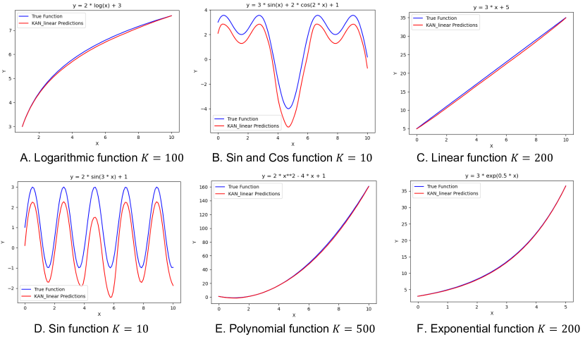
Figure 3: Fourier KAN fits six different functions. A. Logarithmic function $K=100$ B. Sin and Cos function $K=10$ C. Linear function $K=200$ D. Sin function $K=10$ E. Polynomial function $K=500$ F. Exponential function $K=120$

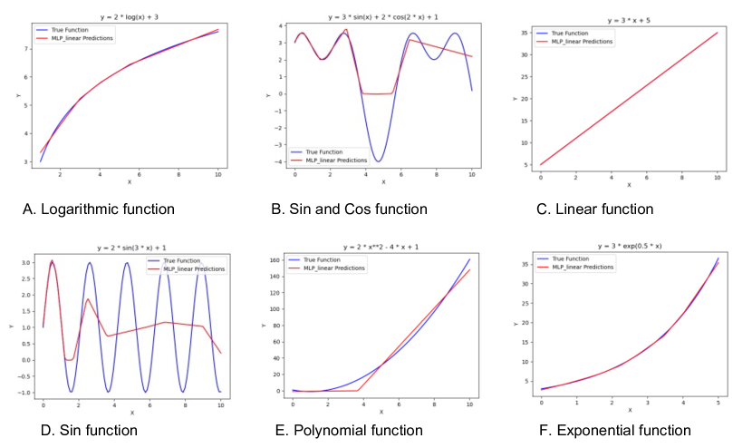
Figure 4: MLP fits six different functions. A. Logarithmic function B. Sin and Cos function C. Linear function D. Sin function E. Polynomial function F. Exponential function

References

- [1] Joseph A DiMasi, Ronald W Hansen, and Henry G Grabowski. The price of innovation: new estimates of drug development costs. Journal of health economics, 22(2):151–185, 2003.
- [2] Bernard Munos. Lessons from 60 years of pharmaceutical innovation. Nature reviews Drug discovery, 8(12):959–968, 2009.
- [3] Joseph A DiMasi, Henry G Grabowski, and Ronald W Hansen. Innovation in the pharmaceutical industry: new estimates of r&d costs. Journal of health economics, 47:20–33, 2016.
- [4] Hongming Chen, Ola Engkvist, Yinhai Wang, Marcus Olivecrona, and Thomas Blaschke. The rise of deep learning in drug discovery. Drug discovery today, 23:1241–1250, 2018.
- [5] HC Stephen Chan, Hanbin Shan, Thamani Dahoun, Horst Vogel, and Shuguang Yuan. Advancing drug discovery via artificial intelligence. Trends in pharmacological sciences, 40(8):592–604, 2019.
- [6] Kristy A Carpenter and Xudong Huang. Machine learning-based virtual screening and its applications to alzheimer’s drug discovery: a review. Current pharmaceutical design, 24(28):3347–3358, 2018.
- [7] Eduardo Habib Bechelane Maia, Letícia Cristina Assis, Tiago Alves De Oliveira, Alisson Marques Da Silva, and Alex Gutterres Taranto. Structure-based virtual screening: from classical to artificial intelligence. Frontiers in chemistry, 8:343, 2020.
- [8] Jun Xia, Lecheng Zhang, Xiao Zhu, Yue Liu, Zhangyang Gao, Bozhen Hu, Cheng Tan, Jiangbin Zheng, Siyuan Li, and Stan Z Li. Understanding the limitations of deep models for molecular property prediction: Insights and solutions. Advances in Neural Information Processing Systems, 36, 2024.
- [9] Z. X. Cang and G. W. Wei. TopologyNet: Topology based deep convolutional and multi-task neural networks for biomolecular property predictions. PLOS Computational Biology, 13(7):e1005690, 2017.
- [10] D. D. Nguyen, Z. X. Cang, and G. W. Wei. A review of mathematical representations of biomolecular data. Physical Chemistry Chemical Physics, 2020.
- [11] Z. X. Cang, L. Mu, and G. W. Wei. Representability of algebraic topology for biomolecules in machine learning based scoring and virtual screening. PLoS computational biology, 14(1):e1005929, 2018.
- [12] Zhenyu Meng and Kelin Xia. Persistent spectral–based machine learning (perspect ml) for protein-ligand binding affinity prediction. Science Advances, 7(19):eabc5329, 2021.
- [13] D. D. Nguyen, T. Xiao, M. L. Wang, and G. W. Wei. Rigidity strengthening: A mechanism for protein–ligand binding. Journal of chemical information and modeling, 57(7):1715–1721, 2017.
- [14] Zixuan Cang and Guo-Wei Wei. Integration of element specific persistent homology and machine learning for protein-ligand binding affinity prediction. International journal for numerical methods in biomedical engineering, 34(2):e2914, 2018.
- [15] D. D. Nguyen and G. W. Wei. AGL-Score: Algebraic graph learning score for protein-ligand binding scoring, ranking, docking, and screening. Journal of chemical information and modeling, 59(7):3291–3304, 2019.
- [16] Jiahui Chen, Rui Wang, Menglun Wang, and Guo-Wei Wei. Mutations strengthened SARS-CoV-2 infectivity. Journal of molecular biology, 432(19):5212–5226, 2020.
- [17] Rui Wang, Yuta Hozumi, Changchuan Yin, and Guo-Wei Wei. Mutations on COVID-19 diagnostic targets. Genomics, 112(6):5204–5213, 2020.
- [18] Kaifu Gao, Duc Duy Nguyen, Meihua Tu, and Guo-Wei Wei. Generative network complex for the automated generation of drug-like molecules. Journal of chemical information and modeling, 60(12):5682–5698, 2020.
- [19] Lukasz Maziarka, Tomasz Danel, Slawomir Mucha, Krzysztof Rataj, Jacek Tabor, and Stanislaw Jastrzebski. Molecule attention transformer. ArXiv, abs/2002.08264, 2020.
- [20] Viraj Bagal, Rishal Aggarwal, PK Vinod, and U Deva Priyakumar. Molgpt: molecular generation using a transformer-decoder model. Journal of Chemical Information and Modeling, 62(9):2064–2076, 2021.
- [21] Shifa Zhong, Jiajie Hu, Xiong Yu, and Huichun Zhang. Molecular image-convolutional neural network (cnn) assisted qsar models for predicting contaminant reactivity toward oh radicals: Transfer learning, data augmentation and model interpretation. Chemical Engineering Journal, 408:127998, 2021.
- [22] Oliver Wieder, Stefan Kohlbacher, Mélaine Kuenemann, Arthur Garon, Pierre Ducrot, Thomas Seidel, and Thierry Langer. A compact review of molecular property prediction with graph neural networks. Drug Discovery Today: Technologies, 37:1–12, 2020.
- [23] Rocío Mercado, Tobias Rastemo, Edvard Lindelöf, Günter Klambauer, Ola Engkvist, Hongming Chen, and Esben Jannik Bjerrum. Graph networks for molecular design. Machine Learning: Science and Technology, 2(2):025023, 2021.
- [24] Qi Liu, Miltiadis Allamanis, Marc Brockschmidt, and Alexander Gaunt. Constrained graph variational autoencoders for molecule design. Advances in neural information processing systems, 31, 2018.
- [25] Yu Rong, Yatao Bian, Tingyang Xu, Weiyang Xie, Ying Wei, Wenbing Huang, and Junzhou Huang. Self-supervised graph transformer on large-scale molecular data. Advances in Neural Information Processing Systems, 33:12559–12571, 2020.
- [26] Menglun Wang, Zixuan Cang, and Guo-Wei Wei. A topology-based network tree for the prediction of protein–protein binding affinity changes following mutation. Nature Machine Intelligence, 2(2):116–123, 2020.
- [27] Cong Shen, Jiawei Luo, and Kelin Xia. Molecular geometric deep learning. Cell Reports Methods, 3(11), 2023.
- [28] Ziming Liu, Yixuan Wang, Sachin Vaidya, Fabian Ruehle, James Halverson, Marin Soljačić, Thomas Y Hou, and Max Tegmark. Kan: Kolmogorov-arnold networks. arXiv preprint arXiv:2404.19756, 2024.
- [29] Zavareh Bozorgasl and Hao Chen. Wav-kan: Wavelet kolmogorov-arnold networks. arXiv preprint arXiv:2405.12832, 2024.
- [30] Remi Genet and Hugo Inzirillo. Tkan: Temporal kolmogorov-arnold networks. arXiv preprint arXiv:2405.07344, 2024.
- [31] Minjong Cheon. Kolmogorov-arnold network for satellite image classification in remote sensing. arXiv preprint arXiv:2406.00600, 2024.
- [32] Jie Shen and Christos A Nicolaou. Molecular property prediction: recent trends in the era of artificial intelligence. Drug Discovery Today: Technologies, 32:29–36, 2019.
- [33] Kenneth Atz, Francesca Grisoni, and Gisbert Schneider. Geometric deep learning on molecular representations. Nature Machine Intelligence, 3(12):1023–1032, 2021.
- [34] Jiaqi Han, Jiacheng Cen, Liming Wu, Zongzhao Li, Xiangzhe Kong, Rui Jiao, Ziyang Yu, Tingyang Xu, Fandi Wu, Zihe Wang, et al. A survey of geometric graph neural networks: Data structures, models and applications. arXiv preprint arXiv:2403.00485, 2024.
- [35] W Patrick Walters and Regina Barzilay. Applications of deep learning in molecule generation and molecular property prediction. Accounts of chemical research, 54(2):263–270, 2020.
- [36] Chunyan Li, Jihua Feng, Shihu Liu, and Junfeng Yao. A novel molecular representation learning for molecular property prediction with a multiple smiles-based augmentation. Computational Intelligence and Neuroscience, 2022, 2022.
- [37] Jing Jiang, Ruisheng Zhang, Zhili Zhao, Jun Ma, Yunwu Liu, Yongna Yuan, and Bojuan Niu. Multigran-smiles: multi-granularity smiles learning for molecular property prediction. Bioinformatics, 38(19):4573–4580, 2022.
- [38] Vıctor Garcia Satorras, Emiel Hoogeboom, and Max Welling. E (n) equivariant graph neural networks. In International conference on machine learning, pages 9323–9332. PMLR, 2021.
- [39] Gabriele Corso, Hannes Stärk, Bowen Jing, Regina Barzilay, and Tommi Jaakkola. Diffdock: Diffusion steps, twists, and turns for molecular docking. arXiv preprint arXiv:2210.01776, 2022.
- [40] Simon Batzner, Albert Musaelian, Lixin Sun, Mario Geiger, Jonathan P Mailoa, Mordechai Kornbluth, Nicola Molinari, Tess E Smidt, and Boris Kozinsky. E (3)-equivariant graph neural networks for data-efficient and accurate interatomic potentials. Nature communications, 13(1):2453, 2022.
- [41] Xiangzhe Kong, Wenbing Huang, and Yang Liu. End-to-end full-atom antibody design. arXiv preprint arXiv:2302.00203, 2023.
- [42] Dong Chen, Kaifu Gao, Duc Duy Nguyen, Xin Chen, Yi Jiang, Guo-Wei Wei, and Feng Pan. Algebraic graph-assisted bidirectional transformers for molecular property prediction. Nature communications, 12(1):3521, 2021.
- [43] Mufei Li, Jinjing Zhou, Jiajing Hu, Wenxuan Fan, Yangkang Zhang, Yaxin Gu, and George Karypis. Dgl-lifesci: An open-source toolkit for deep learning on graphs in life science. ACS omega, 6(41):27233–27238, 2021.
- [44] Kevin Yang, Kyle Swanson, Wengong Jin, Connor Coley, Philipp Eiden, Hua Gao, Angel Guzman-Perez, Timothy Hopper, Brian Kelley, Miriam Mathea, et al. Analyzing learned molecular representations for property prediction. Journal of chemical information and modeling, 59(8):3370–3388, 2019.
- [45] Zhaoping Xiong, Dingyan Wang, Xiaohong Liu, Feisheng Zhong, Xiaozhe Wan, Xutong Li, Zhaojun Li, Xiaomin Luo, Kaixian Chen, Hualiang Jiang, et al. Pushing the boundaries of molecular representation for drug discovery with the graph attention mechanism. Journal of medicinal chemistry, 63(16):8749–8760, 2019.
- [46] Kamal Choudhary and Brian DeCost. Atomistic line graph neural network for improved materials property predictions. npj Computational Materials, 7(1):185, 2021.
- [47] Xiaomin Fang, Lihang Liu, Jieqiong Lei, Donglong He, Shanzhuo Zhang, Jingbo Zhou, Fan Wang, Hua Wu, and Haifeng Wang. Geometry-enhanced molecular representation learning for property prediction. Nature Machine Intelligence, 4(2):127–134, 2022.
- [48] Johannes Gasteiger, Janek Groß, and Stephan Günnemann. Directional message passing for molecular graphs. arXiv preprint arXiv:2003.03123, 2020.
- [49] Johannes Gasteiger, Florian Becker, and Stephan Günnemann. Gemnet: Universal directional graph neural networks for molecules. Advances in Neural Information Processing Systems, 34:6790–6802, 2021.
- [50] Thomas A Halgren. Merck molecular force field. i. basis, form, scope, parameterization, and performance of mmff94. Journal of computational chemistry, 17(5-6):490–519, 1996.
- [51] Shengchao Liu, Mehmet F Demirel, and Yingyu Liang. N-gram graph: Simple unsupervised representation for graphs, with applications to molecules. Advances in neural information processing systems, 32, 2019.
- [52] Weihua Hu, Bowen Liu, Joseph Gomes, Marinka Zitnik, Percy Liang, Vijay Pande, and Jure Leskovec. Strategies for pre-training graph neural networks. In International Conference on Learning Representations, 2019.
- [53] Shengchao Liu, Hanchen Wang, Weiyang Liu, Joan Lasenby, Hongyu Guo, and Jian Tang. Pre-training molecular graph representation with 3d geometry. arXiv preprint arXiv:2110.07728, 2021.
- [54] Yuyang Wang, Jianren Wang, Zhonglin Cao, and Amir Barati Farimani. Molecular contrastive learning of representations via graph neural networks. Nature Machine Intelligence, 4(3):279–287, 2022.
- [55] Gengmo Zhou, Zhifeng Gao, Qiankun Ding, Hang Zheng, Hongteng Xu, Zhewei Wei, Linfeng Zhang, and Guolin Ke. Uni-mol: A universal 3d molecular representation learning framework. In The Eleventh International Conference on Learning Representations, 2023.
- [56] Yishui Li, Wei Wang, Jie Liu, and Chengkun Wu. Pre-training molecular representation model with spatial geometry for property prediction. Computational Biology and Chemistry, 109:108023, 2024.
- [57] Andrei Nikolaevich Kolmogorov. On the representation of continuous functions of many variables by superposition of continuous functions of one variable and addition. In Doklady Akademii Nauk, volume 114, pages 953–956. Russian Academy of Sciences, 1957.
- [58] David A Sprecher. A numerical implementation of kolmogorov’s superpositions. Neural networks, 9(5):765–772, 1996.
- [59] David A Sprecher. A numerical implementation of kolmogorov’s superpositions ii. Neural networks, 10(3):447–457, 1997.
- [60] Jürgen Braun and Michael Griebel. On a constructive proof of kolmogorov’s superposition theorem. Constructive approximation, 30:653–675, 2009.
- [61] Tian Xie and Jeffrey C Grossman. Crystal graph convolutional neural networks for an accurate and interpretable prediction of material properties. Physical review letters, 120(14):145301, 2018.
- [62] Lennart Carleson. On convergence and growth of partial sums of fourier series. Acta Mathematica, 116:135–157, 1966.
- [63] Charles Fefferman. On the convergence of multiple fourier series. Bulletin of the American Mathematical Society, 77:744–745, 1971.
- [64] Zhenqin Wu, Bharath Ramsundar, Evan N Feinberg, Joseph Gomes, Caleb Geniesse, Aneesh S Pappu, Karl Leswing, and Vijay Pande. Moleculenet: a benchmark for molecular machine learning. Chemical science, 9(2):513–530, 2018.
- [65] Bharath Ramsundar, Peter Eastman, Pat Walters, and Vijay Pande. Deep learning for the life sciences: applying deep learning to genomics, microscopy, drug discovery, and more. " O’Reilly Media, Inc.", 2019.
- [66] Shengchao Liu, Hanchen Wang, Weiyang Liu, Joan Lasenby, Hongyu Guo, and Jian Tang. Pre-training molecular graph representation with 3d geometry. In International Conference on Learning Representations, 2022.