Regularized Estimation of High-Dimensional Matrix-Variate Autoregressive Models

Hangjin Jiang¹, Baining Shen¹, Yuzhou Li¹, and Zhaoxing Gao²

¹Center for Data Science, Zhejiang University

²School of Mathematical Sciences, University of Electronic Science and Technology of China

Abstract: Matrix-variate time series data are increasingly popular in economics, statistics, and environmental studies, among other fields. This paper develops regularized estimation methods for analyzing high-dimensional matrix-variate time series using bilinear matrix-variate autoregressive models. The bilinear autoregressive structure is widely used for matrix-variate time series, as it reduces model complexity while capturing interactions between rows and columns. However, when dealing with large dimensions, the commonly used iterated least-squares method results in numerous estimated parameters, making interpretation difficult. To address this, we propose two regularized estimation methods to further reduce model dimensionality. The first assumes banded autoregressive coefficient matrices, where each data point interacts only with nearby points. A two-step estimation method is used: first, traditional iterated least-squares is applied for initial estimates, followed by a banded iterated least-squares approach. A Bayesian Information Criterion (BIC) is introduced to estimate the bandwidth of the coefficient matrices. The second method assumes sparse autoregressive matrices, applying the LASSO technique for regularization. We derive asymptotic properties for both methods as the dimensions diverge and the sample size $T\rightarrow\infty$. Simulations and real data examples demonstrate the effectiveness of our methods, comparing their forecasting performance against common autoregressive models in the literature.

Key words and phrases: Matrix Time Series, High-dimension, Iterated Least-Squares, Band, Lasso

1 Introduction

In recent years, with the development of advanced information technologies, modern data collection and storage capabilities have led to massive amounts of time series data. Multiple and high-dimensional time series are routinely observed in a wide range of applications, including economics, finance, engineering, environmental sciences, medical research, and others. In the past decades, various multivariate time series modeling methods have been studied in the literature. See Tsay (2014) and the references therein for details. Recently, large tensor (or multi-dimensional array) time series data have become increasingly popular in the literature across various fields, including those mentioned. For example, a group of countries will report a set of economic indicators each quarter, forming a matrix-variate (2-dimensional array) time series, with each column representing a country and each row representing an economic indicator. To analyze large and high-dimensional datasets, dimension-reduction techniques have gained popularity for achieving efficient and effective analysis of high-dimensional time series data. Examples include the canonical correlation analysis (CCA) of Box and Tiao (1977) and Gao and Tsay (2019), principal component analysis (PCA) of Stock and Watson (2002), the scalar component model of Tiao and Tsay (1989), and the factor model approach in Bai and Ng (2002), Stock and Watson (2005), Forni et al. (2000, 2005), Pan and Yao, (2008), Lam et al. (2011), Lam and Yao (2012), and Gao and Tsay (2021a, b, 2022), among others. However, all the techniques developed for vector time series cannot be directly applied to matrix-variate time series, and simple vectorization of the matrix data often results in a significant number of estimated parameters, losing the original data structure. Therefore, further analysis methods should be developed to model such complex and dynamic datasets.

Recently, several methods have been developed for analyzing matrix-variate time series data, including factor models in Wang et al. (2019), Chen et al., (2020), Yu et al., (2022), and Gao and Tsay (2021c), as well as the bilinear matrix-variate autoregressive model in Chen et al., (2020). To the best of our knowledge, only the method in Chen et al., (2020) can be directly applied for out-of-sample forecasting, while others primarily focus on dimension reduction of the matrix data structures. Although Chen et al., (2020) introduced effective techniques for estimating autoregressive coefficient matrices and explored their asymptotic properties, these methods are applicable only to matrix-variate time series data with fixed and small dimensions. Given that large-dimensional matrix-variate data are increasingly common in applications, the traditional iterated least-squares methods presented in Chen et al., (2020) may not perform well, and the theoretical results may no longer hold. Therefore, new estimation methods must be considered in such contexts.

This paper represents an extension of the bilinear matrix-variate autoregressive model developed in Chen et al., (2020) and the spatio-temporal data framework in Hsu et al. (2021). We focus on the scenario where the dimensions of matrix-variate data are growing, thereby extending the approach in Chen et al., (2020) to high-dimensional contexts. To facilitate meaningful dimension reduction, we recognize that each observed data point interacts only with a limited number of others. For instance, spatio-temporal data points, such as PM_2.5 observations, may rely primarily on a few neighboring locations. More generally, each observation may dynamically depend on only a subset of other components. Our goal is to identify sparse autoregressive matrices that allow for further dimensional reduction while maintaining interpretability.

In this paper, we propose two regularized estimation methods to reduce the model’s dimensions further. The first method assumes that the autoregressive coefficient matrices are banded, indicating that each observed data point interacts only with a limited number of neighboring points. We introduce a two-step estimation approach: the first step utilizes traditional iterated least-squares to obtain initial estimates, while the second step employs a banded iterated least-squares method. Additionally, we propose using the Bayesian Information Criterion (BIC) to estimate the bandwidths of the coefficient matrices. The second method is similar but assumes that the autoregressive matrices are sparse, applying the LASSO technique for estimation. We derive the asymptotic properties of the proposed methods for diverging dimensions of the matrix-variate data as the sample size $T\rightarrow\infty$. Both simulated and real examples are used to evaluate the performance of our methods in finite samples, comparing them with commonly used techniques in the literature regarding the forecasting ability of autoregressive models.

This paper presents multiple contributions. First, the methods introduced in Chen et al., (2020) are applicable only to matrix-variate time series data with fixed and relatively small dimensions. We extend this model to a high-dimensional environment, offering a broader perspective on matrix-autoregressive models that is increasingly relevant for practitioners as such data become more common in applications. Second, coefficients obtained from traditional least-squares methods can be challenging to interpret due to the large number of parameters associated with higher dimensions. Our approaches, utilizing banded and general sparse structures, address this issue by facilitating meaningful dimensional reductions. The banded approach is particularly well-suited for analyzing spatio-temporal data, as the matrix structure corresponds to the locations of observations, making it reasonable to assume that each data point depends dynamically on only a few neighboring points. Finally, we provide rigorous theoretical analysis, deriving the asymptotic properties of our proposed methods under these circumstances, thereby contributing to the theoretical foundation of this field.

The rest of the paper is organized as follows. We introduce the model and proposed estimation methodology in Section 2 and study the theoretical properties of the proposed model and its associated estimates in Section 3. Numerical studies with both simulated and real data sets are given in Section 4, and Section 5 provides some concluding remarks. All technical proofs are given in an online Supplementary Material. Throughout the article, we use the following notation. For a $p\times 1$ vector ${\mathbf{u}}=(u_{1},...,u_{p})^{\prime},$ $||{\mathbf{u}}||_{2}=\|{\mathbf{u}}^{\prime}\|_{2}=(\sum_{i=1}^{p}u_{i}^{2})^{1/2}$ is the Euclidean norm, $\|{\mathbf{u}}\|_{\infty}=\max_{1\leq i\leq p}|u_{i}|$ is the $\ell_{\infty}$-norm, and ${\mathbf{I}}_{p}$ denotes a $p\times p$ identity matrix. For a matrix ${\mathbf{H}}=(h_{ij})$, $\|{\mathbf{H}}\|_{1}=\max_{j}\sum_{i}|h_{ij}|$, $\|{\mathbf{H}}\|_{\infty}=\max_{i,j}|h_{ij}|$, $\|{\mathbf{H}}\|_{F}=\sqrt{\sum_{i,j}h_{ij}^{2}}$ is the Frobenius norm, $\|{\mathbf{H}}\|_{2}=\sqrt{\lambda_{\max}({\mathbf{H}}^{\prime}{\mathbf{H}})}$ is the operator norm, where $\lambda_{\max}(\cdot)$ denotes for the largest eigenvalue of a matrix, and $\|{\mathbf{H}}\|_{\min}$ is the square root of the minimum non-zero eigenvalue of ${\mathbf{H}}^{\prime}{\mathbf{H}}$. The superscript ^′ denotes the transpose of a vector or matrix. We also use the notation $a\asymp b$ to denote $a=O(b)$ and $b=O(a)$. $\mathbb{E}X$ denotes the expectation of random variable $X$, and ${\mathbf{i}}_{k}$ be the unit vector with the $k$-th element equal to 1. Finally, $C$ is a constant having different values in different contexts.

2 Model and Methodology

2.1 Setting

Let ${\mathbf{Y}}_{t}\in\mathbb{R}^{p_{1}\times p_{2}}$ be an observable $p_{1}\times p_{2}$ matrix-variate time series, we consider the matrix-variate autoregressive model of order $d\geq 1$ (MAR($d$)) introduced by Chen et al., (2020) as follows:

$${\mathbf{Y}}_{t}={\mathbf{A}}_{1}{\mathbf{Y}}_{t-1}{\mathbf{B}}_{1}^{\prime}+...+{\mathbf{A}}_{d}{\mathbf{Y}}_{t-d}{\mathbf{B}}_{d}^{\prime}+{\mathbf{E}}_{t},$$ (2.1)

where ${\mathbf{A}}_{i}$ and ${\mathbf{B}}_{i}$ are the coefficient matrices, and ${\mathbf{E}}_{t}$ is a white noise term. By a similar argument as that in traditional AR models, we may let ${\mathbf{A}}=[{\mathbf{A}}_{1},...,{\mathbf{A}}_{d}]$, ${\mathbf{B}}=[{\mathbf{B}}_{1},...,{\mathbf{B}}_{d}]$, and ${\mathbf{G}}_{t}=\mbox{diag}({\mathbf{Y}}_{t-1},...,{\mathbf{Y}}_{t-d})$, the regression part in Model (2.1) can be written as ${\mathbf{A}}{\mathbf{G}}_{t}{\mathbf{B}}^{\prime}$. Thus, without loss of generality, we only consider the case when $d=1$, i.e., study the following MAR(1) model:

$${\mathbf{Y}}_{t}={\mathbf{A}}{\mathbf{Y}}_{t-1}{\mathbf{B}}^{\prime}+{\mathbf{E}}_{t},$$ (2.2)

where ${\mathbf{Y}}_{t}\in\mathbb{R}^{p_{1}\times p_{2}}$, ${\mathbf{A}}\in\mathbb{R}^{p_{1}\times p_{1}}$, and ${\mathbf{B}}\in\mathbb{R}^{p_{2}\times p_{2}}$ are the coefficient matrices, and ${\mathbf{E}}_{t}\in\mathbb{R}^{p_{1}\times p_{2}}$ is the white noise term.

As discussed in Chen et al., (2020), the coefficient matrices ${\mathbf{A}}$ and ${\mathbf{B}}$ are not uniquely defined due to the identification issue. For example, $({\mathbf{A}},{\mathbf{B}})$ can be replaced by $(c{\mathbf{A}},{\mathbf{B}}/c)$ for some constant $c\neq 0$ without altering the equation in (2.2). Therefore, some identification conditions are required to impose on the coefficients. There are several ways to achieve this, for instance, we may assume $\|{\mathbf{A}}\|_{F}=1$ and $\text{sign}(\mbox{tr}({\mathbf{A}}))=1$ as that in Hsu et al. (2021).

Chen et al., (2020) proposed three methods to estimate the coefficient matrices when the dimensions $p_{1}$ and $p_{2}$ are fixed, which are (1) the Projection method, (2) Iterated least squares approach, and (3) Maximum likelihood estimation (MLE). Asymptotic properties of the estimators are also established therein. However, both their methods and asymptotic theory are derived under finite and fixed dimensions.

In this paper, we consider the estimation of the coefficient matrices in high-dimensional scenarios, i.e., $p_{1},p_{2}\rightarrow\infty$ as $T\rightarrow\infty$. It is widely known that traditional methods usually fail when the dimensions are growing as the sample size increases, and one of the main reasons is that there will be much more parameters to be estimated. Therefore, some interpretable structures are often imposed in a high-dimensional framework. Here, we present the estimation methods under two different cases: 1) the coefficient matrices ${\mathbf{A}}$ and ${\mathbf{B}}$ are banded ones, and 2) ${\mathbf{A}}$ and ${\mathbf{B}}$ are sparse, where the banded coefficients matrices are often used in spatio-temporal data when the observed value of one location only depends on those of a few neighborhoods. On the other hand, in the second scenario, we assume only a small proportion of elements in ${\mathbf{A}}$ and ${\mathbf{B}}$ are non-zero, which serves as a general sparsity condition. Our goal is to estimate the coefficients ${\mathbf{A}}$ and ${\mathbf{B}}$ under such conditions in a high-dimensional framework. We will discuss these two scenarios in the following sections.

2.2 Estimation with the Banded Case

In this section, we consider the scenario that the coefficient matrices ${\mathbf{A}}$ and ${\mathbf{B}}$ are banded ones with bandwidths $k_{1}>0$ and $k_{2}>0$, respectively. That is, we assume that

$$a_{i,j}=0,b_{k,l}=0\,\,\text{for all}\,\,|i-j|>k_{1},|k-l|>k_{2},$$ (2.3)

where ${\mathbf{A}}=(a_{i,j})_{i,j=1}^{p_{1}}$, ${\mathbf{B}}=(b_{k,l})_{k,l=1}^{p_{2}}$, and $k_{1}$ and $k_{2}$ are unknown bandwidths. Our goal is to estimate the coefficient matrices ${\mathbf{A}}$ and ${\mathbf{B}}$, and their corresponding bandwidth parameters $k_{1}$ and $k_{2}$.

We first assume that $k_{1}$ and $k_{2}$ are known, and we will propose a BIC approach to consistently estimate them in subsection 2.2.2 below. For the estimation of the coefficient matrices with banded structures, the procedure can be carried out in a similar way as the iterated least-squares method in Chen et al., (2020). Specifically, we first obtain initial estimators of ${\mathbf{A}}$ and ${\mathbf{B}}$ by the iterated least squares method proposed in Chen et al., (2020). Then we start with the initial estimators, and perform another iterated least squares method to estimate the banded coefficient matrices. For example, we may estimate ${\mathbf{A}}$ and its bandwidths $k_{1}$ when the latest estimator for ${\mathbf{B}}$ is given, and then estimate ${\mathbf{B}}$ and its bandwidths $k_{2}$ by fixing the latest estimator for ${\mathbf{A}}$. We repeat this procedure and the algorithm stops when the estimators converge. A description of the algorithm is outlined in Algorithm 1. Details on Steps 2(a) and 2(b) in Algorithm 1 are given in the following subsections.

Algorithm 1 Estimating algorithm for banded case

1. We use the iterated least-squares method in Chen et al., (2020) to obtain the estimators $\widehat{\mathbf{A}}_{0}$ and $\widehat{\mathbf{B}}_{0}$ for ${\mathbf{A}}$ and ${\mathbf{B}}$, respectively. Denote the initial estimators as $\widehat{\mathbf{B}}^{(0)}=\widehat{\mathbf{B}}_{0}$ and $\widehat{\mathbf{A}}^{(0)}=\widehat{\mathbf{A}}_{0}$.

2. For the $i$-th iteration ($i=1,2,\cdots$),

   1. Fix the estimator $\widehat{\mathbf{B}}^{(i-1)}$ of ${\mathbf{B}}$, the estimator $\widehat{\mathbf{A}}^{(i)}$ of ${\mathbf{A}}$ is obtained by applying the least-squares method to Model (2.2). The estimator of the unknown bandwidth $k_{1}$, denoted by $\widehat{k}_{1}^{(i)}$, is obtained based on a BIC given in section 2.2.2 below.

   2. Fix the estimator $\widehat{\mathbf{A}}^{(i)}$ of ${\mathbf{A}}$, we estimate $\widehat{\mathbf{B}}^{(i)}$ and $\widehat{k}_{2}^{(i)}$ using the same procedure as that in (a).

   3. The iteration stops if the convergence criterion is satisfied, otherwise we go to the next iteration and repeat Steps 2(a)–2(b).

Note that either $\widehat{\mathbf{B}}^{(i-1)}$ in Step 2(a) or $\widehat{\mathbf{A}}^{(i)}$ in Step 2(b) needs to be normalized according to the identification conditions mentioned in Section 2.1. The initial estimator can be either $\widehat{\mathbf{B}}^{(0)}$ or $\widehat{\mathbf{A}}^{(0)}$ which does not influence the properties of the final estimators. For the convergence conditions, there are several useful ones that we can adopt in Step 2(c) of Algorithm 1. For example, we may take the following two convergence criteria:

$$\|\widehat{\mathbf{A}}^{(i)}-\widehat{\mathbf{A}}^{(i-1)}\|_{F}\leq\eta\,\,\text{and}\,\,\|\widehat{\mathbf{B}}^{(i)}-\widehat{\mathbf{B}}^{(i-1)}\|_{F}\leq\eta,$$

or

$$\|\widehat{\mathbf{B}}^{(i)}\otimes\widehat{\mathbf{A}}^{(i)}-\widehat{\mathbf{B}}^{(i-1)}\otimes\widehat{\mathbf{A}}^{(i-1)}\|_{F}\leq\eta,$$

where $\eta>0$ is a prescribed small constant. In practice, we may choose $\eta=10^{-6}$, and simulation results in Section 4 suggest that our algorithm works well in finite samples.

2.2.1 Iterated Least-Squares Estimation

Given ${\mathbf{B}}=\widehat{\mathbf{B}}^{(i-1)}$, in order to obtain the estimator of ${\mathbf{A}}$ and its bandwidth $k_{1}$, we write $\widehat{{\mathbf{Q}}}_{t}={\mathbf{Y}}_{t}\widehat{{\mathbf{B}}}^{(i-1)}{{}^{\prime}}$ and ${{\mathbf{Q}}}_{t}={\mathbf{Y}}_{t}{\mathbf{B}}^{\prime}$, and model (2.2) can be written as

$${\mathbf{Y}}_{t}={\mathbf{A}}\widehat{{\mathbf{Q}}}_{t-1}+{\mathbf{F}}_{1t},{\mathbf{F}}_{1t}={\mathbf{A}}({{\mathbf{Q}}}_{t-1}-\widehat{{\mathbf{Q}}}_{t-1})+{\mathbf{E}}_{t}.$$ (2.4)

Let ${\mathbf{A}}^{\prime}=[{\mathbf{a}}_{1},\cdots,{\mathbf{a}}_{p_{1}}]$, we have, ${\mathbf{Y}}_{t}^{\prime}{\mathbf{i}}_{j}=\widehat{{\mathbf{Q}}}_{t-1}^{\prime}{\mathbf{a}}_{j}+{\mathbf{F}}_{1t}^{\prime}{\mathbf{i}}_{j},j=1,2,\cdots,p_{1}.$

Assuming the bandwidth of ${\mathbf{A}}$ is $k$, then there are $\tau_{j}(k)$ non-zero elements in its $j$-th row ${\mathbf{a}}_{j}$ of ${\mathbf{A}}$, where

$$\tau_{j}(k)=\left\{\begin{array}[]{ll}k+j&{\rm if}~{}~{}~{}j\leq k+1,\\ 2k+1&{\rm if}~{}~{}~{}k+1<j\leq p_{1}-k,\\ p_{1}+k-j+1&{\rm if}~{}~{}~{}p_{1}-k<j\leq p_{1}.\end{array}\right.$$

Let $\boldsymbol{\beta}_{j,k}$ be the $\tau_{j}(k)\times 1$ vector obtained by stacking non-zero elements in ${\mathbf{a}}_{j}$, and ${\mathbf{X}}_{j,t-1}^{k}$ be the corresponding $\tau_{j}(k)$ columns of $\widehat{{\mathbf{Q}}}_{t-1}^{\prime}$. Denote ${\mathbf{v}}_{j}=[{\mathbf{i}}_{j}^{\prime}{\mathbf{Y}}_{2},\cdots,{\mathbf{i}}_{j}^{\prime}{\mathbf{Y}}_{T+1}]^{\prime}\in\mathbb{R}^{Tp_{2}\times 1}$, ${\mathbf{X}}_{j,k}=[{\mathbf{X}}_{j,1}^{k},\cdots,{\mathbf{X}}_{j,T}^{k}]\in\mathbb{R}^{Tp_{2}\times\tau_{j}(k)}$, and $\boldsymbol{f}_{j}=[{\mathbf{i}}_{j}^{\prime}{\mathbf{F}}_{12},\cdots,{\mathbf{i}}_{j}^{\prime}{\mathbf{F}}_{1,T+1}]^{\prime}$, we have

$${\mathbf{v}}_{j}={\mathbf{X}}_{j,k}\boldsymbol{\beta}_{j,k}+\boldsymbol{f}_{j}.$$ (2.5)

Now, it follows from (2.5) that the least-squares estimator of $\boldsymbol{\beta}_{j,k}$ is denoted by $\widehat{\boldsymbol{\beta}}_{j,k}=({\mathbf{X}}_{j,k}^{\prime}{\mathbf{X}}_{j,k})^{-1}{\mathbf{X}}_{j,k}^{\prime}{\mathbf{v}}_{j}$, and the corresponding residual sum of squares can be written as

$$\text{RSS}_{j}(k,{\mathbf{a}}_{j})={\mathbf{v}}_{j}^{\prime}({\mathbf{I}}-{\mathbf{H}}_{{\mathbf{X}}_{j,k}}){\mathbf{v}}_{j},$$ (2.6)

where ${\mathbf{H}}_{{\mathbf{X}}_{j,k}}={\mathbf{X}}_{j,k}({\mathbf{X}}_{j,k}^{\prime}{\mathbf{X}}_{j,k})^{-1}{\mathbf{X}}_{j,k}^{\prime}$ is a hat matrix, which is a function of the unknown bandwidth $k$.

Next, we consider the estimation of ${\mathbf{B}}$ given $\widehat{{\mathbf{A}}}^{(i)}$. Similar to the technique used in (2.4), let $\widehat{{\mathbf{R}}}_{t}=\widehat{{\mathbf{A}}}^{(i)}{\mathbf{Y}}_{t}$ and ${\mathbf{R}}_{t}={\mathbf{A}}{\mathbf{Y}}_{t}$, model (2.2) can be written as

$${\mathbf{Y}}_{t}=\widehat{{\mathbf{R}}}_{t-1}{\mathbf{B}}^{\prime}+{\mathbf{F}}_{2t},{\mathbf{F}}_{2t}=({\mathbf{R}}_{t-1}-\widehat{{\mathbf{R}}}_{t-1}){\mathbf{B}}^{\prime}+{\mathbf{E}}_{t}.$$ (2.7)

Let ${\mathbf{B}}^{\prime}=({\mathbf{b}}_{1},\cdots,{\mathbf{b}}_{p_{2}})$, we have ${\mathbf{Y}}_{t}{\mathbf{i}}_{j}=\widehat{{\mathbf{R}}}_{t-1}{\mathbf{b}}_{j}+{\mathbf{F}}_{2t}{\mathbf{i}}_{j},j=1,2,\cdots,p_{2}.$

Assuming the bandwidth of ${\mathbf{B}}$ is $k$, then there are $\tau_{j}(k)$ non-zero elements in ${\mathbf{b}}_{j}$, where

$$\tau_{j}(k)=\left\{\begin{array}[]{ll}k+j&{\rm if}~{}~{}~{}j\leq k+1,\\ 2k+1&{\rm if}~{}~{}~{}k+1<j\leq p_{2}-k,\\ p_{2}+k-j+1&{\rm if}~{}~{}~{}p_{2}-k<j\leq p_{2}.\end{array}\right.$$

Let $\boldsymbol{\gamma}_{j,k}$ be the $\tau_{j}(k)\times 1$ vector obtained by stacking non-zero elements in ${\mathbf{b}}_{j}$, and ${\mathbf{G}}_{j,t-1}^{k}$ be the corresponding $\tau_{j}(k)$ columns of $\widehat{{\mathbf{R}}}_{t-1}$. Denote ${\mathbf{w}}_{j}=[{\mathbf{i}}_{j}^{\prime}{\mathbf{Y}}_{2}^{\prime},\cdots,{\mathbf{i}}_{j}^{\prime}{\mathbf{Y}}_{T+1}^{\prime}]^{\prime}$, ${\mathbf{G}}_{j,k}=[{\mathbf{G}}_{j,1}^{k};\cdots;{\mathbf{G}}_{j,T}^{k}]$, and $\boldsymbol{r}_{j}=[{\mathbf{i}}_{j}^{\prime}{\mathbf{F}}_{22}^{\prime},\cdots,{\mathbf{i}}_{j}^{\prime}{\mathbf{F}}_{2,T+1}^{\prime}]^{\prime}$, we have

$${\mathbf{w}}_{j}={\mathbf{G}}_{j,k}\boldsymbol{\gamma}_{j,k}+\boldsymbol{r}_{j},$$ (2.8)

and obtain the least-squares estimator of $\boldsymbol{\gamma}_{j,k}$ as $\widehat{\boldsymbol{\gamma}}_{j,k}=({\mathbf{G}}_{j,k}^{\prime}{\mathbf{G}}_{j,k})^{-1}{\mathbf{G}}_{j,k}^{\prime}{\mathbf{w}}_{j}$. The corresponding residual sum of squares is given by

$$\text{RSS}_{j}(k,{\mathbf{b}}_{j})={\mathbf{w}}_{j}^{\prime}({\mathbf{I}}-{\mathbf{H}}_{{\mathbf{G}}_{j,k}}){\mathbf{w}}_{j},$$ (2.9)

where ${\mathbf{H}}_{{\mathbf{G}}_{j,k}}={\mathbf{G}}_{j,k}({\mathbf{G}}_{j,k}^{\prime}{\mathbf{G}}_{j,k})^{-1}{\mathbf{G}}_{j,k}^{\prime}$ is a hat matrix, which is also a function of the unknown bandwidth $k$ as that in (2.6).

2.2.2 Determining the bandwidth

As discussed in Section 2.2.1, the estimation of the unknown coefficients depends on the bandwidth parameters $k_{1}$ and $k_{2}$, which are unknown in practice. In this section, we propose a Bayesian information criterion (BIC) to determine the unknown bandwidth of ${\mathbf{A}}$. We first consider the estimation of the bandwidth $k_{1}$ of ${\mathbf{A}}$. For each prescribed $k_{1}\geq 1$, we may obtain the least-squares estimator of $\widehat{\boldsymbol{\beta}}_{j,k}$ from Model (2.5) as well as the residual-sum of squares in (2.6). For $j=1,...,p_{1}$, we define

$$\text{BIC}_{j}(k)=\log\text{RSS}_{j}(k,{\mathbf{a}}_{j})+\frac{C_{T_{2}}}{T_{2}}\tau_{j}(k)\log(p_{1}\vee T_{2}),$$

where $T_{2}=p_{2}T$, and $C_{T_{2}}=\log\log(T_{2})$. The bandwidth of the $j$-th row of ${\mathbf{A}}$ estimated from $({\mathbf{X}}_{j,k},{\mathbf{v}}_{j})$ is given by

$$\widehat{k}_{1,j}=\arg\min_{1\leq k\leq K}\text{BIC}_{j}(k),$$

where $K$ is a prescribed upper bound of $k$ which may be taken as $\lceil T^{1/2}\rceil$. Finally, the estimated bandwidth of ${\mathbf{A}}$ in the $i$-th iteration of Algorithm 1 is given by $\widehat{k}_{1}^{(i)}=\max_{1\leq j\leq p_{1}}\widehat{k}_{1,j}$, and the estimator for ${\mathbf{A}}$ in the $i$-th iteration is denoted by $\widehat{{\mathbf{A}}}^{(i)}=[\widehat{{\mathbf{a}}}_{1},\widehat{{\mathbf{a}}}_{2},\cdots,\widehat{{\mathbf{a}}}_{p_{1}}]^{\prime}$, where the estimator $\widehat{{\mathbf{a}}}_{j}$ of ${\mathbf{a}}_{j}$ is obtained by replacing the corresponding non-zero elements in ${\mathbf{a}}_{j}$ by $\widehat{\boldsymbol{\beta}}_{j,\widehat{k}_{j}}$.

Similarly, for the estimation of the bandwidth parameter $k_{2}$, we can define the following BIC criterion

$$\text{BIC}_{j}(k)=\log\text{RSS}_{j}(k,{\mathbf{b}}_{j})+\frac{C_{T_{1}}}{T_{1}}\tau_{j}(k)\log(p_{2}\vee T_{1}),$$

where $T_{1}=p_{1}T$, and $C_{T_{1}}=\log\log(T_{1})$. The bandwidth of the $j$-th row of ${\mathbf{B}}$ can be estimated by

$$\widehat{k}_{2,j}=\arg\min_{1\leq k\leq K}\text{BIC}_{j}(k),$$

where $K$ is a prescribed upper bound of $k$ which may be taken as $\lceil T^{1/2}\rceil$. Finally, the bandwidth of ${\mathbf{B}}$, is estimated as $\widehat{k}_{2}^{(i)}=\max_{1\leq j\leq p_{2}}\widehat{k}_{2,j}$ and ${\mathbf{B}}$ is estimated as $\widehat{{\mathbf{B}}}^{(i)}=[\widehat{{\mathbf{b}}}_{1},\widehat{{\mathbf{b}}}_{2},\cdots,\widehat{{\mathbf{b}}}_{p_{2}}]^{\prime}$, where estimator $\widehat{{\mathbf{b}}}_{j}$ of ${\mathbf{b}}_{j}$ is obtained by replacing corresponding non-zero elements in ${\mathbf{b}}_{j}$ by $\widehat{\boldsymbol{\beta}}_{j,\widehat{k}_{j}}$, which is similar as that in estimating $k_{1}$.

In practice, the upper bound $K>0$ in the BICs defined above is a prescribed integer. Our numerical results show that the procedure is insensitive to the choice of $K$ so long as $K>k_{1}$ and $K>k_{2}$. In practice, we may take $K$ to be $\min([T^{1/2}],[p_{1}^{1/2}],[p_{2}^{1/2}])$ or choose $K$ by checking the curvature of BIC${}_{i}(k)$ directly.

2.3 Estimation with Sparse Coefficient Matrices

In this section, we consider the estimation of the coefficient matrices in model (2.2) under the scenario that the coefficients are sparse, i.e., we assume that ${\mathbf{A}}$ and ${\mathbf{B}}$ are sparse in the sense that only a few elements within are nonzero. Note that we may apply the properties of the Kronecker product to model (2.2), and rewrite the model in the following two ways:

$$\textnormal{vec}({\mathbf{Y}}_{t})=(({\mathbf{B}}{\mathbf{Y}}_{t-1}^{\prime})\otimes{\mathbf{I}}_{p_{1}})\textnormal{vec}({\mathbf{A}})+\textnormal{vec}({\mathbf{E}}_{t}),$$ (2.10)

and

$$\textnormal{vec}({\mathbf{Y}}_{t}^{\prime})=(({\mathbf{A}}{\mathbf{Y}}_{t-1})\otimes{\mathbf{I}}_{p_{2}})\textnormal{vec}({\mathbf{B}})+\textnormal{vec}({\mathbf{E}}_{t}^{\prime}),$$ (2.11)

where $\textnormal{vec}(\cdot)$ is the vectorization operator that stacks all the columns of a matrix into a vector in order.

Let ${\mathbf{y}}_{t}=\textnormal{vec}({\mathbf{Y}}_{t})$ and ${\mathbf{y}}_{t}^{*}=\textnormal{vec}({\mathbf{Y}}_{t}^{\prime})$, it is possible to estimate ${\mathbf{A}}$ when ${\mathbf{B}}$ is known in (2.10) and to estiamte ${\mathbf{B}}$ when ${\mathbf{A}}$ is known in (2.11). For any consistent estimators $\widehat{\mathbf{B}}$ and $\widehat{\mathbf{A}}$ for ${\mathbf{B}}$ and ${\mathbf{A}}$, respectively, we may define ${\mathbf{Z}}_{t-1}=({\mathbf{B}}{\mathbf{Y}}_{t-1}^{\prime})\otimes{\mathbf{I}}_{p_{1}}$ and $\widehat{\mathbf{Z}}_{t-1}=(\widehat{{\mathbf{B}}}{\mathbf{Y}}_{t-1}^{\prime})\otimes{\mathbf{I}}_{p_{1}}$. Similarly, we may also define ${\mathbf{Z}}_{t-1}^{*}=({\mathbf{A}}{\mathbf{Y}}_{t-1})\otimes{\mathbf{I}}_{p_{2}}$ and $\widehat{\mathbf{Z}}_{t-1}^{*}=(\widehat{{\mathbf{A}}}{\mathbf{Y}}_{t-1})\otimes{\mathbf{I}}_{p_{2}}$. In view of the spare structures of the coefficient matrices, we may adopt some penalized method such as the Lasso to obtain the estimators.

Specifically, similar to the approach in the banded case in Section 2.2, we first obtain the initial estimators of ${\mathbf{A}}$ and ${\mathbf{B}}$ by applying the alternative least squares method proposed by Chen et al., (2020). Starting with these initial estimators, we may apply the Lasso technique to estimate ${\mathbf{A}}$ by replacing ${\mathbf{B}}$ with its latest estimator, and then obtain the Lasso estimate of ${\mathbf{B}}$ by replacing ${\mathbf{A}}$ with its latest estimator. For example, denote the estimate for ${\mathbf{B}}$ as $\widehat{\mathbf{B}}^{(i-1)}$ in the $i$-th iteration, we solve the following optimization problem:

$$\widehat{\boldsymbol{\alpha}}=\arg\min_{\boldsymbol{\alpha}\in R^{p_{1}^{2}}}\left\{\frac{1}{T}\sum_{t=2}^{T}\|{\mathbf{y}}_{t}-\widehat{\mathbf{Z}}_{t-1}\boldsymbol{\alpha}\|_{2}^{2}+\lambda_{1,T}\|\boldsymbol{\alpha}\|_{1}\right\},$$ (2.12)

where $\widehat{\mathbf{B}}$ is equal to $\widehat{\mathbf{B}}^{(i-1)}$ in $\widehat{\mathbf{Z}}_{t-1}$ and $\lambda_{1,T}>0$ is a tuning parameter. Then the estimator $\widehat{\mathbf{A}}^{(i)}$ is obtained by reverting the $\widehat{\boldsymbol{\alpha}}$ to a $p_{1}\times p_{1}$ matrix according to the way $\textnormal{vec}(\cdot)$ is performed. Similarly, $\widehat{\boldsymbol{\beta}}$ is obtained by solving the following optimization problem:

$$\widehat{\boldsymbol{\beta}}=\arg\min_{\boldsymbol{\beta}\in R^{p_{2}^{2}}}\left\{\frac{1}{T}\sum_{t=2}^{T}\|{\mathbf{y}}_{t}^{*}-\widehat{\mathbf{Z}}_{t-1}^{*}\boldsymbol{\beta}\|_{2}^{2}+\lambda_{2,T}\|\boldsymbol{\beta}\|_{1}\right\},$$ (2.13)

where $\widehat{\mathbf{A}}$ is equal to $\widehat{\mathbf{A}}^{(i)}$ in $\widehat{\mathbf{Z}}_{t-1}^{*}$. Then, the estimator $\widehat{\mathbf{B}}^{(i)}$ is obtained by reverting the $\widehat{\boldsymbol{\beta}}$ to a $p_{2}\times p_{2}$ matrix as before. We can repeat this procedure until convergence. The estimation procedure is summarized in Algorithm 2. The convergence criteria are similar to those in Algorithm 1, and we do not repeat them to save space.

Algorithm 2 Estimating algorithm for sparse case

1. Obtain $\widehat{\mathbf{A}}_{0}$ and $\widehat{\mathbf{B}}_{0}$ by the method in Chen et al., (2020), denoted as $\widehat{\mathbf{B}}^{(0)}=\widehat{\mathbf{B}}_{0}$ and $\widehat{\mathbf{A}}^{(0)}=\widehat{\mathbf{A}}_{0}$, respectively.

2. For the $i$-th iteration ($i=1,2,...$),

   1. Fix ${\mathbf{B}}=\widehat{\mathbf{B}}^{(i-1)}$, apply Lasso to (2.12) and obtain $\widehat{\mathbf{A}}^{(i)}$,

   2. Fix ${\mathbf{A}}=\widehat{\mathbf{A}}^{(i)}$, apply Lasso to (2.13) and obtain $\widehat{\mathbf{B}}^{(i)}$,

   3. The iteration stops if the convergence criterion is satisfied, otherwise we go to the next iteration and repeat Steps 2(a)–2(b).

3 Theoretical Properties

In this section, we establish the asymptotic properties of the estimators proposed in Section 2. We begin by outlining the regular conditions necessary for the theoretical proofs, followed by the statement of the asymptotic theorems. All proofs for the theorems are provided in an online Supplementary Material.

3.1 Regular Conditions

We introduce some notations first. A process $\textnormal{vec}({\mathbf{Y}}_{t})$ is $\alpha$-mixing if

$$\alpha_{p}(k)=\sup_{i}\sup_{A\in\mathcal{F}_{-\infty}^{i},B\in\mathcal{F}_{i+k}^{\infty}}|\mathbb{P}(A\cap B)-\mathbb{P}(A)\mathbb{P}(B)|\rightarrow 0,$$

where $\mathcal{F}_{l}^{k}$ is the $\sigma$-field generated by $\{\textnormal{vec}({\mathbf{Y}}_{t}):l\leq t\leq k\}$. For $i=1,2$, define $C_{i,\alpha}(S_{i})=\{\Delta\in R^{p_{i}^{2}}:\|\Delta_{S_{i}^{c}}\|_{1}\leq\alpha\|\Delta_{S_{i}}\|_{1}\}$, where $S_{i}$ is a subset of $\{1,2,...,p_{i}^{2}\}$ and $\Delta_{S_{i}}$ is the vector of $\Delta$ restricted on the positions of $S_{i}$ and the other elements on indexes of $S_{i}^{c}$ are zero. Now, we introduce some assumptions for Model (2.2).

• For ${{\mathbf{Y}}_{t}}=\{y_{ijt}\}$, we assume

  1. The process ${\text{vec}({\mathbf{Y}}_{t})}$ is $\alpha$-mixing with the mixing coefficient satisfying the condition $\alpha_{p}(k)\leq\exp(-ck^{\gamma_{1}})$ for some $\gamma_{1}>0$.

  2. $\sup_{i,j,t}\mathbb{P}(|y_{ij,t}|>s)\leq\exp(1-s^{\gamma_{2}})$ for $s>0$ and some $\gamma_{2}>0$.

• The innovations $\{{\mathbf{E}}_{t}=(e_{ijt})\}$ are independent and identically distributed (i.i.d.) with mean 0, and

  1. $\frac{1}{p_{1}}\sum_{i=1}^{p_{1}}{\mathbb{E}e_{ijt}^{2}}\rightarrow\sigma_{1}^{2}$ for $j=1,2,\cdots,p_{2}$ and $\frac{1}{p_{2}}\sum_{j=1}^{p_{2}}{\mathbb{E}e_{ijt}^{2}}\rightarrow\sigma_{2}^{2}$, for $i=1,2,\cdots,p_{1}$.

  2. $\sup_{i,j,t}\mathbb{P}(|e_{ij,t}|>s)\leq\exp(1-s^{\gamma_{3}})$ for $s>0$ and some $\gamma_{3}>0$.

• $\rho({\mathbf{A}})\rho({\mathbf{B}})<1$, where $\rho({\mathbf{A}})$ and $\rho({\mathbf{B}})$ are the spectral radii of ${\mathbf{A}}$ and ${\mathbf{B}}$, respectively.

• For any two sub-columns of ${\mathbf{Q}}_{t}^{\prime}$ (or ${\mathbf{R}}_{t}$), denoted by ${\mathbf{W}}_{t}$ and ${\mathbf{U}}_{t}$, and ${\mathbf{W}}_{t}\neq{\mathbf{U}}_{t}$, let $p=p_{2}$ (or $p_{1}$), $\Sigma_{{\mathbf{U}}}=p^{-1}\mathbb{E}{\mathbf{U}}_{t}^{\prime}{\mathbf{U}}_{t}$, $\Sigma_{{\mathbf{W}}{\mathbf{U}}}=p^{-1}\mathbb{E}{\mathbf{W}}_{t}^{\prime}{\mathbf{U}}_{t}$, and $\Sigma_{{\mathbf{W}}}=p^{-1}\mathbb{E}{\mathbf{W}}_{t}^{\prime}{\mathbf{W}}_{t}$, there exists some positive constants $\lambda_{1}\leq\lambda_{2}$, such that $\lambda_{1}\leq\lambda_{\min}(\Sigma_{{\mathbf{U}}})\leq\lambda_{\max}(\Sigma_{{\mathbf{U}}})\leq\lambda_{2}$, and $\lambda_{1}\leq\lambda_{\min}(\Sigma_{{\mathbf{W}}}-\Sigma_{{\mathbf{W}}{\mathbf{U}}}\Sigma_{{\mathbf{U}}}^{-1}\Sigma_{{\mathbf{W}}{\mathbf{U}}}^{\prime})\leq\lambda_{\max}(\Sigma_{{\mathbf{W}}}-\Sigma_{{\mathbf{W}}{\mathbf{U}}}\Sigma_{{\mathbf{U}}}^{-1}\Sigma_{{\mathbf{W}}{\mathbf{U}}}^{\prime})\leq\lambda_{2}$.

• For the banded matrix ${\mathbf{A}}$, $|a_{i,i-k_{1}}|$ or $|a_{i,i+k_{1}}|$, $i=1,2,\cdots,p_{1}$, is greater than $\{C_{T_{2}}k_{1}T_{2}^{-1}\log(p_{1}\vee T_{2})\}^{1/2}$ with $T_{2}=p_{2}T$ and $C_{T_{2}}=\log\log T_{2}$; Similarly, for the banded matrix ${\mathbf{B}}$, $|b_{i,i-k_{2}}|$ or $|b_{i,i+k_{2}}|$, $i=1,2,\cdots,p_{2}$, is greater than $\{C_{T_{1}}k_{2}T_{1}^{-1}\log(p_{2}\vee T_{1})\}^{1/2}$ with $T_{1}=p_{1}T$ and $C_{T_{1}}=\log\log T_{1}$.

• For matrices ${\mathbf{A}}$ and ${\mathbf{B}}$, $a_{i,j}$ and $b_{i,j}$ are bounded uniformly, and $\|{\mathbf{A}}^{k}\|_{2}\leq\delta^{k}$ and $\|{\mathbf{B}}^{k}\|_{2}\leq\delta^{k}$ for $k\geq 2$, where $\delta\in(0,1)$ is independent of $p_{1}$, $p_{2}$, and $k$.

• Let $S_{0}$ be a subset of $\{1,2,...,p_{1}^{2}\}$ with cardinality $s_{0}$ consisting of the indexes of the non-zero components in $\boldsymbol{\alpha}=\textnormal{vec}({\mathbf{A}})$, and $S_{0}^{c}$ be its complement. Let ${\mathbf{Z}}_{t}=({\mathbf{B}}{\mathbf{Y}}_{t}^{\prime})\otimes{\mathbf{I}}_{p_{1}}$, (a) when $p_{1}$ is finite, there exists a constant $C_{2}>0$ such that $\lambda_{min}\{\mathbb{E}({\mathbf{Z}}_{t}{\mathbf{Z}}_{t}^{\prime})\}>C_{2}$; (b) when $p_{1}$ is diverging, the matrix ${\mathbf{Z}}:=({\mathbf{Z}}_{1},...,{\mathbf{Z}}_{T})^{\prime}$ satisfies the restricted eigenvalues condition, $\frac{1}{T}\|{\mathbf{Z}}\Delta\|_{2}^{2}\geq\kappa\|\Delta\|_{2}^{2}$, for all $\Delta\in C_{1,3}(S_{0})$. Similar assumptions also hold for ${\mathbf{Z}}_{t}^{*}$ defined in Section 2.3.

• For matrices ${\mathbf{A}}$ and ${\mathbf{B}}$, $\lambda_{1}<\lambda_{\min}\{p_{2}^{-1}\mathbb{E}[({\mathbf{A}}{\mathbf{Y}}_{t})\otimes({\mathbf{Y}}_{t}{\mathbf{B}}^{\prime})]\}<\lambda_{\max}\{p_{2}^{-1}\mathbb{E}[({\mathbf{A}}{\mathbf{Y}}_{t})\otimes({\mathbf{Y}}_{t}{\mathbf{B}}^{\prime})]\}<\lambda_{2}$.

Conditions A1(a-b) are standard for econometric time series models. Condition A2(a) ensures the row and column variances of ${\mathbf{E}}_{t}$ exits, and condition A2(b) is used to bound a new time series built on ${\mathbf{E}}_{t}$ and ${\mathbf{Y}}_{t}$. Condition A3 ensures that model (2.2) is stationary and causal, as shown in proposition 1 in Chen et al., (2020). Conditions A4-A7 are imposed to prove the consistency of the estimated bandwidth by BIC in Section 2.2.2. Condition A5 ensures that the bandwidth is asymptotically identifiable, since both $\{C_{T_{2}}k_{1}T_{2}^{-1}\log(p_{1}\vee T_{2})\}^{1/2}$ and $\{C_{T_{1}}k_{2}T_{1}^{-1}\log(p_{2}\vee T_{1})\}^{1/2}$ is the minimum magnitude of a non-zero coefficient to be identifiable, see, e.g. Gao et al. (2019). Condition A7(a) indicates that the regressors have a non-singular covariance and the least-squares estimators are well defined when $p_{1}$ is finite. Condition A5(b) is the well-known restricted-eigenvalue condition in Lasso regressions; see Chapter 6 in Buhlmann and Van De Geer (2011). The condition in Condition A7(b) can also be replaced by a more general Restricted Strong Convexity condition that is commonly used in high-dimensional regularized estimation problems. See Chapter 9 of Wainwright (2019) for details.

3.2 Asymptotic properties

In this section, we study the theoretical properties of the proposed method, i.e., the convergence of Algorithm 1 and Algorithm 2 in Section 2. Since we take estimators, $\widehat{{\mathbf{A}}}_{0}$ and $\widehat{{\mathbf{B}}}_{0}$, from the iterated least squares in Chen et al., (2020) as our initials in Algorithm 1 and Algorithm 2, we first study the convergence rate of $\widehat{{\mathbf{A}}}_{0}$ and $\widehat{{\mathbf{B}}}_{0}$. Let $\Sigma$ be the covariance matrix of $\textnormal{vec}({\mathbf{E}}_{t})$, and define $\boldsymbol{H}=\mathbb{E}\left(\boldsymbol{W}_{t}\boldsymbol{W}_{t}^{\prime}\right)+\boldsymbol{\gamma}\boldsymbol{\gamma}^{\prime}$, where $\boldsymbol{W}_{t}^{\prime}=[({\mathbf{B}}{\mathbf{Y}}_{t}^{\prime})\otimes{\mathbf{I}}:{\mathbf{I}}\otimes({\mathbf{A}}{\mathbf{Y}}_{t})]\in\mathbb{R}^{p_{1}p_{2}\times(p_{1}^{2}+p_{2}^{2})}$ and $\boldsymbol{\gamma}=(\textnormal{vec}({\mathbf{A}})^{\prime},\boldsymbol{0})^{\prime}\in\mathbb{R}^{p_{1}^{2}+p_{2}^{2}}$. Let $p=\max\{p_{1},p_{2}\}$, we have following result for $\widehat{{\mathbf{A}}}_{0}$ and $\widehat{{\mathbf{B}}}_{0}$.

Proposition 1.

Let conditions A1-A3 hold. If ${\mathbf{A}}$, ${\mathbf{B}}$, $\Sigma$ are nonsingular, $\lambda_{\min}({\mathbf{H}})\geq\lambda_{h}>0$, and $T,p_{1},p_{2}\rightarrow\infty$, then,

$$\|\widehat{{\mathbf{A}}}_{0}-{\mathbf{A}}\|_{F}^{2}+\|\widehat{{\mathbf{B}}}_{0}-{\mathbf{B}}\|_{F}^{2}=O_{p}(\frac{p_{1}^{2}p_{2}}{T}+\frac{p_{2}^{2}p_{1}}{T}).$$

Remark 3.1.

(1) When the dimensions of ${\mathbf{Y}}_{t}$, $p_{1}$ and $p_{2}$, are fixed, the convergence rate of $\|\widehat{{\mathbf{A}}}_{0}-{\mathbf{A}}\|_{F}^{2}$ and $\|\widehat{{\mathbf{B}}}_{0}-{\mathbf{B}}\|_{F}^{2}$ are both of order $O_{p}(1/T)$. This recovers the low-dimensional case.
(2) According to this Proposition, we have $\|\widehat{{\mathbf{A}}}_{0}-{\mathbf{A}}\|_{F}^{2}+\|\widehat{{\mathbf{B}}}_{0}-{\mathbf{B}}\|_{F}^{2}\rightarrow 0$ if $p_{1}^{2}p_{2}/T\rightarrow 0$ and $p_{2}^{2}p_{1}/T\rightarrow 0$, which can be simplified as $pp_{1}p_{2}/T\rightarrow 0$.

Next, we show the convergence rate of estimators for ${\mathbf{A}}$ and ${\mathbf{B}}$ in Algorithm 1 by assuming the bandwidth $k_{1}$ and $k_{2}$ are known and fixed. Theorem 3.1 below shows that estimators from Algorithm 1 are consistent when $p^{3}/T\rightarrow 0$.

Theorem 3.1.

Assume conditions A1-A6 and A8 hold. Let $\widehat{{\mathbf{B}}}^{(i-1)}$ be the latest estimator of ${\mathbf{B}}$ in Algorithm 1 with $\widehat{{\mathbf{B}}}^{(0)}=\widehat{{\mathbf{B}}}_{0}$ and $i\geq 1$. We have, for $i>1$,

$$\|\widehat{{\mathbf{A}}}^{(i)}-{\mathbf{A}}\|_{F}^{2}=O_{p}(\eta)\text{ and }\|\widehat{{\mathbf{B}}}^{(i)}-{\mathbf{B}}\|_{F}^{2}=O_{p}(\eta),$$

and,

$$\|\widehat{{\mathbf{A}}}^{(i)}-{\mathbf{A}}\|_{2}^{2}=O_{p}(\eta)\text{ and }\|\widehat{{\mathbf{B}}}^{(i)}-{\mathbf{B}}\|_{2}^{2}=O_{p}(\eta),$$

where $\eta=\|\widehat{{\mathbf{B}}}^{(i-1)}-{\mathbf{B}}\|_{F}^{2}$.

Remark 3.2.

(i) In this theorem, Algorithm 1 is assumed to begin estimating ${\mathbf{A}}$ by fixing ${\mathbf{B}}$ at its most recent estimate. However, the same conclusion will hold if we reverse the estimation order.
(ii) In the first iteration, we take $\widehat{{\mathbf{B}}}^{(0)}=\widehat{{\mathbf{B}}}_{0}$, by Proposition 1, we have $\|\widehat{{\mathbf{B}}}_{0}-{\mathbf{B}}\|_{F}^{2}\rightarrow 0$ when $pp_{1}p_{2}/T\rightarrow 0$. The condition $pp_{1}p_{2}/T\rightarrow 0$ also ensures that the error of ${\mathbf{A}}^{(i)}$ is primarily influenced by the error arising from approximating ${\mathbf{B}}$ with its latest estimate.

Theorem 3.1 is based on the assumption that the bandwidths are known, which is often not the case in real-world problems. However, if consistent estimators for these two unknown bandwidths exist, Theorem 3.1 remains valid. We will now demonstrate the consistency of the estimated bandwidths in Algorithm 1.

Theorem 3.2.

Assume conditions A1-A6 hold. Let $\widehat{{\mathbf{B}}}^{(i-1)}$ be the latest estimator of ${\mathbf{B}}$ in Algorithm 1 with $\widehat{{\mathbf{B}}}^{(0)}=\widehat{{\mathbf{B}}}_{0}$. For $i>1$, if $p^{5}/T\rightarrow 0$, then

$$P(\widehat{k}_{1}^{(i)}=k_{1})\rightarrow 1,\text{ and }P(\widehat{k}_{2}^{(i)}=k_{2})\rightarrow 1,\text{ as }T,p_{1},p_{2}\rightarrow\infty.$$

Remark 3.3.

(i) In Theorem 3.1, $k_{1}$ and $k_{2}$ are assumed to be fixed, since model (2.2) is useful only when $k_{1}$ and $k_{2}$ are small and finite. However, Theorem 3.1 still holds when $k_{1}$ and $k_{2}$ diverges to $\infty$ along with $T,p_{1},p_{2}$ so long as $k_{1}=o\{C_{T_{2}}^{-1}T_{2}/\log(p_{1}\vee T_{2})\}$, and $k_{2}=o\{C_{T_{1}}^{-1}T_{1}/\log(p_{2}\vee T_{1})\}$, where $T_{2}=p_{2}T$, $C_{T_{2}}=\log\log T_{2}$, $T_{1}=p_{1}T$, and $C_{T_{1}}=\log\log T_{1}$. See the proof of Theorem 3.1 in Supplementary Material.
(ii) In this theorem, Algorithm 1 is assumed to begin estimating ${\mathbf{A}}$ by fixing ${\mathbf{B}}$ at its most recent estimate. However, the same conclusion holds if we reverse the estimation order.

Next, we examine the convergence rate of Algorithm2 for estimating ${\mathbf{A}}$ and ${\mathbf{B}}$ in the sparse case. Similar to Algorithm1, Algorithm 2 also begins with $\widehat{{\mathbf{A}}}_{0}$ and $\widehat{{\mathbf{B}}}_{0}$, which are derived from the iterated least squares method in Chen et al., (2020).

Theorem 3.3.

Assume conditions A1-A3 and A6-A7 hold. Let $\widehat{{\mathbf{B}}}^{(i-1)}$ be the latest estimator of ${\mathbf{B}}$ in Algorithm 2 with $\widehat{{\mathbf{B}}}^{0}=\widehat{{\mathbf{B}}}_{0}$ and $i\geq 1$, we have,

$$\|\widehat{{\mathbf{A}}}^{(i)}-{\mathbf{A}}\|_{2}=O_{p}(\lambda_{1}\sqrt{s_{0}})\text{ and }\|\widehat{{\mathbf{B}}}^{(i)}-{\mathbf{B}}\|_{2}=O_{p}(\lambda_{2}\sqrt{s_{0}}),$$

where $\lambda_{1},\lambda_{2}\asymp\sqrt{\frac{p_{1}p_{2}p}{T}}$, and $s_{0}=|S_{0}|$.

Similar to the results in the banded case, Theorem 3.3 shows that the estimated sparse coefficients are consistent under the condition that $pp_{1}p_{2}/T\rightarrow 0$ for finite sparsity $0<s_{0}<\infty$.

4 Numerical Results

In this section, we examine the finite sample properties of the proposed method and provide real data examples to evaluate its forecasting performance compared to the alternative least-squares (ALSE) method proposed by Chen et al., (2020). In Section 4.1, we conduct Monte Carlo experiments to demonstrate the convergence of the proposed methods in estimating the coefficient matrices under two scenarios, alongside comparisons with the estimators obtained using the ALSE method. In Section 4.2, we apply our method to two real data examples.

4.1 Simulation

This section outlines our methodology for evaluating the finite sample properties of the proposed methods through Monte-Carlo experiments. The observed data matrix ${\mathbf{Y}}_{t}$ are simulated from model (2.2) under different conditions for matrices ${\mathbf{A}}$ and ${\mathbf{B}}$, and each entry in the white noise ${\mathbf{E}}_{t}$ is generated from the standard normal distribution, with $\mbox{Cov}(\text{vec}({\mathbf{E}}_{t}))={\mathbf{I}}_{p_{1}p_{2}}$. Through these simulations, we aim to demonstrate the convergence of our proposed methods in comparison with the ALSE method, as the sample size increases. Furthermore, we examine the accuracy of our proposed methods in estimating unknown bandwidths under the banded cases. The impact of penalty parameters on the estimation results is also investigated under the sparse cases. All of the results are obtained by conducting $100$ independent replications.

To study the convergence of the estimators for matrices ${\mathbf{A}}$ and ${\mathbf{B}}$, some identification conditions are required to impose on the coefficients. In this experiment, we assume $\|{\mathbf{A}}\|_{F}=1$ and $\text{sign}(\text{tr}({\mathbf{A}}))=1$. The convergence criteria of the iterations in our algorithms are specified as $\|\widehat{{\mathbf{A}}}^{(i+1)}-\widehat{{\mathbf{A}}}^{(i)}\|_{F}<10^{-6}$ and $\|\widehat{{\mathbf{B}}}^{(i+1)}-\widehat{{\mathbf{B}}}^{(i)}\|_{F}<10^{-6}$.

4.1.1 Banded case

This section presents a comprehensive analysis to investigate the performance of Algorithm 1. We will study the convergence of the estimators under the scenarios that we start with either $\widehat{\mathbf{A}}^{(0)}$ or $\widehat{\mathbf{B}}^{(0)}$ as initial estimates. Additionally, we examine the accuracy of the bandwidth estimation and the algorithm’s convergence as the sample size $T$ increases.

For each configuration of $(p_{1},p_{2},k_{1},k_{2},T)$, we generate ${\mathbf{Y}}_{t}$ according to model (2.2). Specifically, for given dimensions $p_{1}$, $p_{2}$, and bandwidths $k_{1}$ and $k_{2}$, the observed data ${\mathbf{Y}}_{t}$ are simulated according to model (2.2), where the entries of ${\mathbf{A}}$ and ${\mathbf{B}}$ are generated as follows: (1) for entries of ${\mathbf{A}}$, $\{a_{i,j}:|i-j|\leq k_{1}\}$ are generated independently from $U[-1,1]$, and other elements are zero. We re-scale ${\mathbf{A}}$ such that $\|{\mathbf{A}}\|_{F}$ = 1; (2) for entries of ${\mathbf{B}}$, $\{b_{i,j}:|i-j|\leq k_{2}\}$ are generated independently from $U[-1,1]$, and other elements are zero. We re-scale ${\mathbf{B}}$ so that $\rho=\rho({\mathbf{A}})\rho({\mathbf{B}})=0.5$. The white noise ${\mathbf{E}}_{t}$ are generated from standard normal distribution with $\mbox{Cov}(\text{vec}({\mathbf{E}}_{t}))={\mathbf{I}}_{p_{1}p_{2}}$.

Firstly, we examine the convergence of Algorithm 1 is insensitive to the choice of the initial estimators. Note that there are two iteration orders that may occur in Algorithm 1. We may first estimate ${\mathbf{A}}$ for given initial estimator $\widehat{\mathbf{B}}^{(0)}$, or estimate ${\mathbf{B}}$ for given $\widehat{\mathbf{A}}^{(0)}$. We denote the estimated coefficient matrices via these two procedures by $(\widehat{{\mathbf{A}}}_{1},\widehat{{\mathbf{B}}}_{1})$ and $(\widehat{{\mathbf{A}}}_{2},\widehat{{\mathbf{B}}}_{2})$, respectively. The dimensions are set as $(p_{1},p_{2})=(6,4),(8,5)$ and $(9,6)$ with bandwidths $(k_{1},k_{2})=(2,1)$ for each $(p_{1},p_{2})$. The mean, median, and maximum of $\log_{10}{(\|\widehat{{\mathbf{A}}}_{1}-\widehat{{\mathbf{A}}}_{2}\|_{F})}$ and $\log_{10}{(\|\widehat{{\mathbf{B}}}_{1}-\widehat{{\mathbf{B}}}_{2}\|_{F})}$ are reported in Table 1. From Table 1 we see that the convergence of the estimators is insensitive to the choice of the initial estimators that we use in Algorithm 1. On the other hand, the reported errors in Table 1 are all less than $-6$, which is in accordance with the convergence criteria where the upper bound $\eta$ is chosen as $10^{-6}$ in Section 2.

Table 1: The mean, median, and maximum of $\log_{10}{(\|\widehat{{\mathbf{A}}}_{1}-\widehat{{\mathbf{A}}}_{2}\|_{F})}$ and $\log_{10}{(\|\widehat{{\mathbf{B}}}_{1}-\widehat{{\mathbf{B}}}_{2}\|_{F})}$, where $(\widehat{{\mathbf{A}}}_{1},\widehat{{\mathbf{B}}}_{1})$ and $(\widehat{{\mathbf{A}}}_{2},\widehat{{\mathbf{B}}}_{2})$ are obtained by starting with the initial estimators $\widehat{\mathbf{B}}^{(0)}$ and $\widehat{\mathbf{A}}^{(0)}$ in Algorithm 1, respectively.

	$\log_{10}{(\|\widehat{{\mathbf{A}}}_{1}-\widehat{{\mathbf{A}}}_{2}\|_{F})}$			$\log_{10}{(\|\widehat{{\mathbf{B}}}_{1}-\widehat{{\mathbf{B}}}_{2}\|_{F})}$
$(p_{1},p_{2})$	Mean	Median	Maximum	Mean	Median	Maximum
$(6,4)$	-7.67	-7.75	-7.09	-6.64	-6.85	-6.39
$(8,5)$	-7.57	-7.62	-7.19	-6.38	-6.43	-6.01
$(9,6)$	-7.42	-7.52	-6.91	-6.23	-6.36	-6.00

Second, we show the accuracy of Algorithm 1 in estimating the unknown bandwidths $k_{1}$ and $k_{2}$. The empirical frequencies of the events $\{\widehat{k}_{1}=k_{1}\}$ and $\{\widehat{k}_{2}=k_{2}\}$ are reported in Table 2, where we set $(k_{1},k_{2})=(1,1)$ and $(2,1)$ and the sample size $T=100,200,400$ and $800$. For a fixed sample size $T$ and the bandwidths $(k_{1},k_{2})$, the dimensions $(p_{1},p_{2})$ are set to $(6,4)$, $(8,5)$, and $(9,6)$. Results in Table 2 show that the accuracy of estimated $\widehat{k}_{1}$ and $\widehat{k}_{2}$ is pretty satisfactory, and it increases with sample size $T$ for each $(p_{1},p_{2},k_{1},k_{2})$ in most cases.

Table 2: Accuracy of Algorithm 1 in estimating unknown bandwidths under different settings, where $E_{1}$ and $E_{2}$ represent the empirical frequencies of the events $\{\widehat{k}_{1}=k_{1}\}$ and $\{\widehat{k}_{2}=k_{2}\}$, respectively.

	$T=100$		$T=200$		$T=400$		$T=800$
$(p_{1},p_{2})$	$E_{1}$	$E_{2}$	$E_{1}$	$E_{2}$	$E_{1}$	$E_{2}$	$E_{1}$	$E_{2}$
$(k_{1},k_{2})=(1,1)$
$(6,4)$	100	100	100	100	100	100	100	100
$(8,5)$	100	99	100	99	100	100	100	100
$(9,6)$	98	99	100	99	100	100	100	100
$(k_{1},k_{2})=(2,1)$
$(6,4)$	98	100	100	100	100	100	100	100
$(8,5)$	99	100	100	100	100	100	100	100
$(9,6)$	99	100	100	100	100	100	100	100

Next, we show the convergence pattern of Algorithm 1 under different configurations of $(p_{1},p_{2},k_{1},k_{2})$ as the sample size $T$ increases. We also compare the estimation accuracy with the ALSE method in Chen et al., (2020). The estimation errors for ${\mathbf{A}}$ and ${\mathbf{B}}$, denoted by $\log(\|\widehat{{\mathbf{A}}}-{\mathbf{A}}\|_{F})$ and $\log(\|\widehat{{\mathbf{B}}}-{\mathbf{B}}\|_{F})$, respectively, are reported in Table 3, where $(p_{1},p_{2})=(6,4)$ and $(9,6)$, the sample size $T=200,500,1000,2000$, and the bandwidths $(k_{1},k_{2})=(2,1)$. For each setting, we consider two scenarios that $\rho({\mathbf{A}})\rho({\mathbf{B}})=0.5$ and $0.8$ to show the results are consistent for different strengths of the coefficient matrices. From Table 3, we see that estimation errors obtained by the proposed method and the ALSE all decrease as the sample size increase for each configuration, which is in line with our theoretical results. On the other hand, we also see that the estimation error obtained by our proposed method is smaller than that by the ALSE, implying that our estimation procedure is more accurate than the ALSE.

Furthermore, we define ${\mathbf{S}}:={\mathbf{B}}\otimes{\mathbf{A}}$ and $\widehat{\mathbf{S}}:=\widehat{\mathbf{B}}\otimes\widehat{\mathbf{A}}$, using the distance $\log(|\widehat{\mathbf{S}}-{\mathbf{S}}|_{F})$ to evaluate the overall performance of our proposed method. For simplicity, we set the dimensions $(p_{1},p_{2})=(6,4)$ and $(9,6)$, and the bandwidths $(k_{1},k_{2})$ to $(1,1)$ and $(2,1)$ for each $(p_{1},p_{2})$. We fix $\rho({\mathbf{A}})\rho({\mathbf{B}})=0.5$ in this experiment, and the boxplots of the estimated errors $\log(|\widehat{\mathbf{S}}-{\mathbf{S}}|_{F})$ are shown in Figure 1. It is clear that both methods converge under these settings, and our proposed Algorithm 1 performs better than the ALSE method in terms of estimation errors, which aligns with our theoretical results.

Table 3: The average estimation errors of the coefficient matrices by Algorithm 1 and ALSE.

		Algorithm 1				ALSE
$(p_{1},p_{2})$	$\rho$	T = 200	500	1000	2000	T = 200	500	1000	2000
$\log(\|\widehat{{\mathbf{A}}}-{\mathbf{A}}\|_{F})$
$(6,4)$	0.5	-1.960	-2.454	-2.842	-3.214	-1.830	-2.298	-2.637	-2.999
$(6,4)$	0.8	-2.536	-3.022	-3.354	-3.677	-2.295	-2.777	-3.097	-3.462
$(9,6)$	0.5	-1.191	-1.691	-2.236	-2.733	-1.215	-1.666	-2.009	-2.348
$(9,6)$	0.8	-2.115	-2.499	-2.813	-3.089	-1.798	-2.267	-2.596	-2.949
$\log(\|\widehat{{\mathbf{B}}}-{\mathbf{B}}\|_{F})$
$(6,4)$	0.5	-1.701	-2.154	-2.474	-2.805	-1.401	-1.882	-2.208	-2.558
$(6,4)$	0.8	-1.758	-2.232	-2.564	-2.945	-1.479	-1.961	-2.318	-2.696
$(9,6)$	0.5	-1.314	-1.799	-2.154	-2.513	-0.860	-1.328	-1.704	-2.058
$(9,6)$	0.8	-1.444	-1.967	-2.268	-2.615	-0.987	-1.477	-1.826	-2.175
$\log(\|\widehat{{\mathbf{S}}}-{\mathbf{S}}\|_{F})$
$(6,4)$	0.5	-0.950	-1.434	-1.806	-2.166	-0.778	-1.252	-1.591	-1.946
$(6,4)$	0.8	-1.139	-1.617	-1.953	-2.295	-0.892	-1.369	-1.705	-2.076
$(9,6)$	0.5	-0.394	-0.885	-1.388	-1.855	-0.290	-0.753	-1.110	-1.454
$(9,6)$	0.8	-0.735	-1.151	-1.464	-1.751	-0.381	-0.858	-1.195	-1.546

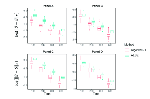
Figure 1: Error of Kronecker product $\log(\|\widehat{{\mathbf{S}}}-{\mathbf{S}}\|_{F})$ of ALSE and Algorithm 1 under different settings of ($p_{1},p_{2}$) and $(k_{1},k_{2})$. Panel A: $(p_{1},p_{2})=(6,4)$, $(k_{1},k_{2})=(1,1)$; Panel B: $(p_{1},p_{2})=(6,4)$, $(k_{1},k_{2})=(2,1)$; Panel C: $(p_{1},p_{2})=(9,6)$, $(k_{1},k_{2})=(2,1)$; Panel D: $(p_{1},p_{2})=(9,6)$, $(k_{1},k_{2})=(3,2)$; Results are reported from 100 independent repetitions.

4.1.2 Sparse case

This section evaluates the performance of Algorithm 2 in estimating sparse coefficient matrices. First, we assess its ability to recover the non-zero elements of matrices ${\mathbf{A}}$ and ${\mathbf{B}}$. The tuning parameters $\lambda_{1,T}$ and $\lambda_{2,T}$ in equations (2.12) and (2.13) significantly influence the sparsity of ${\mathbf{A}}$ and ${\mathbf{B}}$, respectively. It is important to note that if these parameters are adjusted in each iteration of Algorithm 2, the algorithm will not converge, as the objective function changes with the tuning parameters. Therefore, we select the tuning parameters in the first iteration and keep them fixed for subsequent iterations. In practice, tuning parameters are usually chosen through cross-validation (CV). The R package glmnet offers two options: (1) sdCV, which selects $\lambda_{1,T}$ ($\lambda_{2,T}$) as the largest value of $\lambda$ such that the corresponding CV error is within 1 standard error of the minimum, and (2) mCV, which selects $\lambda_{1,T}$ ($\lambda_{2,T}$) as the value of $\lambda$ that minimizes the CV error.

Alternatively, tuning parameters can also be selected based on variable selection stability, as discussed in Meinshausen and Buhlmann, (2010) and Sun et al. (2013). The key idea is to choose tuning parameters that ensure stability in the variable selection process of the penalized regression model. We employ the Kappa Selection Criterion (KSC) proposed by Sun et al. (2013) to select $\lambda_{1,T}$ and $\lambda_{2,T}$. Here, variable selection stability is defined as the expected value of Cohen’s kappa coefficient (Cohen,, 1960) between active sets obtained from two independent and identical datasets. For instance, consider problem (2.12). Given $\lambda_{1,T}=\lambda$, KSC first estimates the variable selection stability $S(\lambda)$ by randomly partitioning the samples ${({\mathbf{y}}_{t},\widehat{\mathbf{Z}}_{t-1}):t=2,\cdots,T}$ into two subsets, repeating this process $B$ times. Then, $\lambda_{1,T}$ is chosen as $\widehat{\lambda}_{1,T}=\min{\lambda:\frac{S(\lambda)}{\max_{\lambda^{\prime}}S(\lambda^{\prime})}\geq 1-\alpha_{T}}$, where we set $B=50$ and $\alpha_{T}=0.4$. In summary, there are three methods for selecting tuning parameters in Algorithm 2, and their impact on the algorithm’s performance is discussed in the following sections.

In our simulations, the coefficient matrices ${\mathbf{A}}\in\mathbb{R}^{p_{1}\times p_{1}}$ and ${\mathbf{B}}\in\mathbb{R}^{p_{2}\times p_{2}}$ are generated as follows: For a given dimension $p_{1}$, let $r_{1}$ be the proportion of nonzero entries in ${\mathbf{A}}$. For each row of ${\mathbf{A}}$, $\left\lfloor\frac{p_{1}}{2}\right\rfloor$ entries are generated from $U[1,2]$, and the remaining $p_{1}-\left\lfloor\frac{p_{1}}{2}\right\rfloor$ entries are generated from $U[-2,-1]$. Next, $p_{1}-\left\lfloor r_{1}p_{1}\right\rfloor$ entries are set to zero, and the elements are randomly rearranged to form one row of ${\mathbf{A}}$. Finally, we rescale ${\mathbf{A}}$ so that $|{\mathbf{A}}|_{F}=1$. The procedure for generating ${\mathbf{B}}$ follows the same steps as for ${\mathbf{A}}$, except that ${\mathbf{B}}$ is rescaled to satisfy $\rho({\mathbf{A}})\rho({\mathbf{B}})=0.9$.

To measure the accuracy of Algorithm 2 in recovering non-zero elements, we define the following sets for ${\mathbf{A}}=(a_{i,j})$ and $\widehat{\mathbf{A}}=(\widehat{a}_{i,j})$:

$$S_{1}=\{(i,j)|a_{i,j}=0,\widehat{a}_{i,j}=0\}, S_{2}=\{(i,j)|a_{i,j}=0,\widehat{a}_{i,j}\neq 0\},$$

$$S_{3}=\{(i,j)|a_{i,j}\neq 0,\widehat{a}_{i,j}\neq 0\}, S_{4}=\{(i,j)|a_{i,j}\neq 0,\widehat{a}_{i,j}=0\}.$$

The recovery accuracy for non-zero elements in ${\mathbf{A}}$ is then defined as

$$\text{cr}(\widehat{\mathbf{A}})=\frac{|S_{1}|+|S_{3}|}{p_{1}\times p_{1}},$$ (4.1)

which represents the proportion of correctly estimated zero and non-zero entries in $\widehat{\mathbf{A}}$ relative to ${\mathbf{A}}$. The recovery accuracy for non-zero elements in ${\mathbf{B}}=(b_{i,j})$ is defined similarly.

Table 4 reports $\text{cr}(\widehat{\mathbf{A}})$ and $\text{cr}(\widehat{\mathbf{B}})$ under different settings and tuning methods from 100 independent replications. Algorithm 2 shows varying performance depending on the tuning method. Specifically, tuning with sdCV results in the highest accuracy for recovering non-zero elements but also the largest error in $\log(|\widehat{\mathbf{S}}-{\mathbf{S}}|_{F})$. In contrast, tuning with mCV yields the best accuracy for $\log(|\widehat{\mathbf{S}}-{\mathbf{S}}|_{F})$ but the worst recovery accuracy. Finally, tuning with KSC provides a balanced performance, achieving comparable results in both recovery accuracy and the error in $\log(|\widehat{\mathbf{S}}-{\mathbf{S}}|_{F})$, making it a well-rounded choice.

Table 4: The performance of Algorithm 2 under different settings and different tuning methods: sdCV, mCV and KSC.

			sdCV			mCV			KSC
$(p_{1},p_{2})$	$T$	$E_{\text{alse}}$	$\text{cr}(\widehat{\mathbf{A}})$	$\text{cr}(\widehat{\mathbf{B}})$	$E_{\text{lasso}}$	$\text{cr}(\widehat{\mathbf{A}})$	$\text{cr}(\widehat{\mathbf{B}})$	$E_{\text{lasso}}$	$\text{cr}(\widehat{\mathbf{A}})$	$\text{cr}(\widehat{\mathbf{B}})$	$E_{\text{lasso}}$
$(6,4)$	100	-0.558	0.979	0.999	-0.324	0.691	0.725	-0.848	0.931	0.965	-0.797
	200	-0.906	0.987	0.999	-0.579	0.682	0.688	-1.211	0.930	0.951	-1.116
	400	-1.260	0.996	1	-0.751	0.706	0.716	-1.573	0.929	0.962	-1.525
	800	-1.616	0.998	1	-0.963	0.703	0.716	-1.920	0.936	0.966	-1.856
$(9,6)$	100	-0.247	0.93	0.983	0.001	0.663	0.674	-0.495	0.914	0.930	-0.287
	200	-0.602	0.956	0.990	-0.248	0.662	0.661	-0.856	0.915	0.944	-0.628
	400	-0.962	0.974	0.997	-0.463	0.671	0.663	-1.228	0.918	0.945	-0.990
	800	-1.305	0.981	0.999	-0.668	0.66	0.661	-1.558	0.913	0.937	-1.340

Next, we compare our estimators with those obtained by the ALSE method from Chen et al., (2020) in terms of estimation errors. Figure 2 presents the box plot of $\log(|\widehat{\mathbf{S}}-{\mathbf{S}}|_{F})$ from 100 independent replications. Detailed results on the estimation errors of $\widehat{\mathbf{A}}$, $\widehat{\mathbf{B}}$, and $\widehat{\mathbf{S}}$ using the KSC tuning method are reported in Table 5, while results for the sdCV and mCV tuning methods are shown in Table S1 and S2, respectively. Figure 2 and Table 5 indicate that the estimators produced by Algorithm 2 generally outperform those from the ALSE method, as the Lasso solutions yield smaller estimation errors in most cases. This suggests that the proposed procedure generates more accurate estimators. Additionally, consistent with previous findings, Algorithm 2 tuned with KSC shows comparable performance to that tuned with mCV, and significantly outperforms the sdCV-tuned version, as seen in Figure 2, Table 5, Table S1, and Table S2. It also performs better than ALSE (Figure 2).

In summary, Algorithm 2 tuned by KSC demonstrates satisfactory performance in both recovery accuracy and estimation error, outperforming ALSE with significantly sparser coefficient matrices that are easier to interpret. Therefore, we recommend it for real data applications. From this point forward, we will refer to Algorithm 2 as Algorithm 2 tuned by KSC.

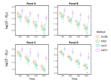
Figure 2: Estimation error $\log(\|\widehat{{\mathbf{S}}}-{\mathbf{S}}\|_{F})$ of ALSE and Algorithm 2 with different tuning methods (sdCV, mCV and KSC) under different settings of ($p_{1},p_{2}$) and $(r_{1},r_{2})$. Panel A: $(p_{1},p_{2})=(6,4)$, $(r_{1},r_{2})=(0.3,0.3)$; Panel B: $(p_{1},p_{2})=(6,4)$, $(r_{1},r_{2})=(0.4,0.4)$; Panel C: $(p_{1},p_{2})=(9,6)$, $(k_{1},k_{2})=(0.3,0.3)$; Panel D: $(p_{1},p_{2})=(9,6)$, $(k_{1},k_{2})=(0.4,0.4)$. Results are reported from 100 independent repetitions.

Table 5: The estimation errors of the estimators obtained by ALSE and Algorithm 2 with tuning parameters method KSC.

		Algorithm 2 tunned by KSC				ALSE
$(p_{1},p_{2})$	$\rho$	T = 100	500	1000	2000	T = 100	500	1000	2000
$\log(\|\widehat{\mathbf{A}}-{\mathbf{A}}\|_{F})$
$(6,4)$	0.5	-1.603	-2.173	-2.553	-2.96	-1.465	-1.903	-2.243	-2.597
$(6,4)$	0.9	-2.364	-2.853	-3.225	-3.571	-2.196	-2.645	-2.993	-3.344
$(9,6)$	0.5	-1.753	-2.308	-2.710	-3.127	-1.546	-2.003	-2.355	-2.712
$(9,6)$	0.9	-2.634	-3.124	-3.494	-3.893	-2.334	-2.793	-3.144	-3.495
$\log(\|\widehat{\mathbf{B}}-{\mathbf{B}}\|_{F})$
$(6,4)$	0.5	-1.319	-1.817	-2.162	-2.511	-1.265	-1.802	-2.152	-2.508
$(6,4)$	0.9	-1.420	-1.902	-2.253	-2.612	-1.425	-1.921	-2.272	-2.631
$(9,6)$	0.5	-0.913	-1.383	-1.737	-2.076	-0.880	-1.375	-1.730	-2.070
$(9,6)$	0.9	-1.059	-1.521	-1.874	-2.219	-1.064	-1.538	-1.887	-2.231
$\log(\|\widehat{\mathbf{S}}-{\mathbf{S}}\|_{F})$
$(6,4)$	0.5	-0.843	-1.389	-1.755	-2.134	-0.736	-1.216	-1.561	-1.918
$(6,4)$	0.9	-0.990	-1.479	-1.840	-2.192	-0.891	-1.359	-1.706	-2.063
$(9,6)$	0.5	-0.469	-0.989	-1.366	-1.742	-0.324	-0.798	-1.151	-1.505
$(9,6)$	0.9	-0.697	-1.174	-1.534	-1.902	-0.523	-0.988	-1.338	-1.687

4.2 Real Data Examples

In this section, we apply the proposed regularized estimation methods to two real-world examples. We utilize three iterative algorithms: the ALSE method from Chen et al., (2020), Algorithm 1, and Algorithm 2 to estimate the coefficient matrices ${\mathbf{A}}$ and ${\mathbf{B}}$ in Model (2.1). We then examine the out-of-sample forecasting errors produced by the MAR(1) model using parameters estimated by the three approaches. The empirical findings demonstrate that our proposed algorithms achieve a high degree of sparsity in modeling the matrix-variate data, resulting in a significant reduction in model parameters. Furthermore, our methods outperform the ALSE method in terms of out-of-sample forecast errors.

4.2.1 Wind Speed Data

In this example, we apply our methodology to a wind speed dataset consisting of the east–west component of the wind speed vector over a region between latitudes $14^{\circ}$S and $16^{\circ}$N and longitudes $145^{\circ}$E and $175^{\circ}$E in the western Pacific Ocean. The data records the average wind speed every 6 hours on a $17\times 17$ grid (covering 289 locations) from November 1992 to February 1993, resulting in $T=480$ and $p_{1}=p_{2}=17$. Previous studies by Hsu et al. (2012) and Hsu et al. (2021) have shown evidence of non-stationary spatial dependence, while indicating temporal stationarity with positive temporal correlations.

The observed data was divided into training data $\{{\mathbf{Y}}_{1},\dots,{\mathbf{Y}}_{400}\}$ and validation data $\{{\mathbf{Y}}_{401},\dots,{\mathbf{Y}}_{480}\}$. We apply the three iterative estimation methods (ALSE, Algorithm 1, and Algorithm 2) to obtain the estimated coefficients $\widehat{\mathbf{A}}$ and $\widehat{\mathbf{B}}$ in the model (2.2). To evaluate the performances of these methods, we calculate the average prediction mean-squared error (PMSE).

$$\text{PMSE}=\frac{1}{289\times 80}\sum_{t=400}^{479}\|\widehat{\mathbf{Y}}_{t+1}-{\mathbf{Y}}_{t+1}\|_{F},$$

and the average prediction mean-absolute error (PMAE)

$$\text{PMAE}=\frac{1}{289\times 80}\sum_{t=400}^{479}\|\widehat{\mathbf{Y}}_{t+1}-{\mathbf{Y}}_{t+1}\|_{1},$$

on the validation data, where $\widehat{\mathbf{Y}}_{t+1}=\widehat{\mathbf{A}}{\mathbf{Y}}_{t}\widehat{\mathbf{B}}^{\prime}$. Furthermore, the sparsity of the coefficient matrices estimated by these methods, in terms of the proportions of zero entries in each matrix and the number of iteration steps, is reported in Table 6. From Table 6, we see that our proposed Algorithm 1 under the banded case and Algorithm 2 under the sparse case perform better than the ALSE method in terms of both PMSE and PMAE. Moreover, the degree of sparsity of the coefficient matrices estimated by our methods is much higher than that by the ALSE method, which implies that our methods greatly simplify the model. In general, Algorithm 2 with $\lambda_{1}=\lambda_{2}=0.1$ in the Lasso estimation performed best among the three methods. The bandwidths of $\widehat{\mathbf{A}}$ and $\widehat{\mathbf{B}}$ chosen by the proposed BIC are 4 and 5, respectively. The heat maps of the $\widehat{\mathbf{A}}$ and $\widehat{\mathbf{B}}$ estimated by the three methods are shown in Figure 3, which clearly illustrate the sparsity of the parameters estimated by our methods.

Table 6: The performance of the three different methods on wind speed data.

Method	PMSE	PMAE	Sparsity of $\widehat{\mathbf{A}}$	Sparsity of $\widehat{\mathbf{B}}$	Iteration step
ALSE	0.16612	0.20007	0	0	45
Algorithm 1	0.16563	0.19983	0.6851	0.7578	8
Algorithm 2	0.16341	0.19665	0.7647	0.8651	6

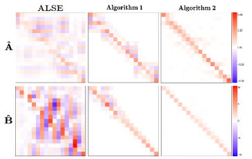
Figure 3: The coefficient matrices estimated by ALSE, Algorithm 1, and Algorithm 2 from U-wind dataset. The first row shows results of $\widehat{\mathbf{A}}$, and the second row shows those of $\widehat{\mathbf{B}}$ obtained by different methods.

4.2.2 Economic Indicator Data

The data in this example consists of quarterly observations of four economic indicators: the long-term interest rate (first-order differenced series), GDP growth (first-order log differenced of the GDP series), total manufacturing production growth (first-order log differenced of the production series), and the total consumer price index (growth from the previous period). These indicators are sourced from five countries: Canada, France, Germany, the United Kingdom, and the United States. The dataset spans from the first quarter of 1990 to the fourth quarter of 2016, resulting in a $4\times 5$ matrix-valued time series with a time length of $T=107$. This data has been previously studied in Chen et al., (2020), and we follow the same data arrangement order for the five countries and four economic indicators. The data can be obtained from the Organisation for Economic Co-operation and Development (OECD) at https://data.oecd.org/.

To eliminate seasonal effects, we adjusted the seasonality of the Consumer Price Index (CPI) by subtracting the sample quarterly means. In Figure 4, we present these adjusted data, with rows and columns corresponding to different economic indicators and countries.

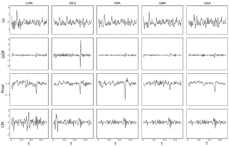
Figure 4: Time series of four indicators: Long-term interest rate(first order difference), GDP growth(log difference), Total manufacture Production growth(log difference), and Total CPI growth from last period subtracted the sample quarterly means from five countries.

We compare the out-of-sample rolling forecast performances of the MAR model (2.2) estimated using the three iterative methods mentioned above. The out-of-sample rolling forecasting begins from $t=87$ to $t=106$. For each time point, we fit the model using the data ${{\mathbf{Y}}_{1},{\mathbf{Y}}_{2},\dots,{\mathbf{Y}}_{t}}$ to obtain the estimated coefficient matrices $\widehat{\mathbf{A}}$ and $\widehat{\mathbf{B}}$. We then compute the predictive value $\widehat{\mathbf{Y}}_{t+1}=\widehat{\mathbf{A}}{\mathbf{Y}}_{t}\widehat{\mathbf{B}}^{\prime}$, as well as the 1-norm predictive error $\|\widehat{\mathbf{Y}}_{t+1}-{\mathbf{Y}}_{t+1}\|_{1}$ and the F-norm predictive error $\|\widehat{\mathbf{Y}}{t+1}-{\mathbf{Y}}_{t+1}\|_{F}$. The averages of the 1-norm and F-norm errors from $t=87$ to $t=106$ for the three iterative methods are reported in Table 7. Notably, both our Lasso iterative method and the banded iterative method outperform the ALSE method from Chen et al., (2020).

Table 7: The Out-sample rolling forecast performances of the three methods(ALSE, Algorithm 1 and Algorithm 2) on Economic indicator data.

	ALSE	Algorithm 1	Algorithm 2
MAE	0.7249358	0.7094906	0.7027468
MSE	0.8533359	0.8378350	0.8236744

5 Conclusion

In this paper, we studied statistical estimators for high-dimensional matrix-valued autoregressive models under two different settings: when the parameter matrix is banded or sparse. We established the asymptotic properties of these estimators. Both simulations and real data analyses demonstrate the advantages of our new methods over existing ones. The proposed method can be treated as another option in the toolbox for modeling high-dimensional matrix-variate time series and the dynamic models can be useful to practitioners who are interested in out-of-sample forecasting.

¹Center for Data Science, Zhejiang University. E-mail: {jianghj,12335035,12235025}@zju.edu.cn

²School of Mathematical Sciences, University of Electronic Science and Technology of China. E-mail: zhaoxing.gao@uestc.edu.cn

References

• Ahn and Horenstein (2013) Ahn, S. C., and, Horenstein, A. R. (2013). Eigenvalue ratio test for the number of factors. Econometrica, 81(3), 1203โ€“1227.
• Andrews (1991) Andrews, D. W. (1991). Heteroskedasticity and autocorrelation consistent covariance matrix estimation. Econometrica, 59, 817โ€“858.
• Bai (2003) Bai J. (2003) Inferential theory for factor models of large dimensions. Econometrica, 71(1), 135โ€“171.
• Bai and Ng (2002) Bai, J. and Ng, S. (2002). Determining the number of factors in approximate factor models. Econometrica, 70, 191โ€“221.
• Black (1986) Black, F. (1986). Noise. The Journal of Finance, 41(3), 528โ€“543.
• Box and Tiao (1977) Box, G. E. P. and Tiao, G. C. (1977). A canonical analysis of multiple time series. Biometrika, 64, 355โ€“365.
• Changย etย al., (2017) Chang, J., Yao, Q. and Zhou, W. (2017). Testing for high-dimensional white noise using maximum cross-correlations. Biometrika, 104(1), 111โ€“127.
• Chenย etย al., (2020) Chen, E.Y., Tsay, R.S., and Chen, R. (2020). Constrained factor models for high-dimensional matrix-variate time series. Journal of the American Statistical Association, 115(530), 775โ€“793.
• Chenย etย al., (2020) Chen, R., Xiao, H., and Yang, D. (2020). Autoregressive models for matrix-valued time series. Journal of Econometrics (forthcoming).
• Cohen, (1960) Cohen, J. (1960) A coefficient of agreement for nominal scales. Educational and Psychological Measurement, 20, 37-46.
• Ding and Cook, (2018) Ding, S. and Cook, R. D. (2018). Matrix variate regressions and envelope models. Journal of the Royal Statistical Society: Series B, 80(2), 387โ€“408.
• Fama and French (2015) Fama, E. F. and French, K. R. (2015). A five-factor asset pricing model. Journal of Financial Economics, 116(1), 1โ€“22.
• Fan et al. (2013) Fan, J., Liao, Y., and Mincheva, M. (2013). Large covariance estimation by thresholding principal orthogonal complements (with discussion). Journal of the Royal Statistical Society, Series B, 75(4), 603โ€“680.
• Forni et al. (2000) Forni, M., Hallin, M., Lippi, M. and Reichlin, L. (2000). Reference cycles: the NBER methodology revisited (No. 2400). Centre for Economic Policy Research.
• Forni et al. (2005) Forni, M., Hallin, M., Lippi, M. and Reichlin, L. (2005). The generalized dynamic factor model: one-sided estimation and forecasting. Journal of the American Statistical Association, 100(471), 830โ€“840.
• Gao (2020) Gao, Z. (2020). Segmenting high-dimensional matrix-valued time series via sequential transformations. arXiv:2002.03382.
• Gao et al. (2019) Gao, Z., Ma, Y., Wang, H. and Yao, Q. (2019). Banded spatio-temporal autoregressions. Journal of Econometrics, 208(1), 211โ€“230.
• Gao and Tsay (2019) Gao, Z. and Tsay, R. S. (2019). A structural-factor approach for modeling high-dimensional time series and space-time data. Journal of Time Series Analysis, 40, 343โ€“362.
• Gao and Tsay (2021a) Gao, Z. and Tsay, R. S. (2021a). Modeling high-dimensional unit-root time series. International Journal of Forecasting, 37(4), 1535โ€“1555.
• Gao and Tsay (2021b) Gao, Z. and Tsay, R. S. (2021b). Modeling high-dimensional time series: a factor model with dynamically dependent factors and diverging eigenvalues. Journal of the American Statistical Association, forthcoming.
• Gao and Tsay (2021c) Gao, Z. and Tsay, R. S. (2021c). A two-way transformed factor model for matrix-variate time series. Econometrics and Statistics, forthcoming.
• Gao and Tsay (2022) Gao, Z. and Tsay, R. S. (2022). Divide-and-conquer: a distributed hierarchical factor approach to modeling large-scale time series data. Journal of the American Statistical Association, forthcoming.
• Guo et al. (2016) Guo, S., Wang, Y. and Yao, Q. (2016). High dimensional and banded vector autoregression. Biometrika, 103(4), 889โ€“903.
• Han et al. (2020) Han, Y., Chen, R., Yang, D., and Zhang, C. H. (2020). Tensor factor model estimation by iterative projection. arXiv preprint arXiv:2006.02611.
• Hauglustaine and Ehhalt (2002) Hauglustaine, D. A., and Ehhalt, D. H. (2002). A threeโ€dimensional model of molecular hydrogen in the troposphere. Journal of Geophysical Research: Atmospheres, 107(D17), ACH-4.
• Hsu et al. (2021) Hsu, N. J., Huang, H. C., and Tsay, R. S. (2021). Matrix autoregressive spatio-temporal models. Journal of Computational and Graphical Statistics, 30(4), 1143โ€“1155.
• Hsu et al. (2012) Hsu, N. J., Chang, Y. M., and Huang, H. C. (2012). A group lasso approach for nonโ€stationary spatialโ€“temporal covariance estimation. Environmetrics, 23, 12-23.
• Hosking, (1980) Hosking, J. R. (1980). The multivariate portmanteau statistic. Journal of the American Statistical Association, 75(371), 602โ€“608.
• Hung et al. (2012) Hung, H., Wu, P., Tu, I., and Huang, S. (2012). On multilinear principal component analysis of order-two tensors. Biometrika, 99(3), 569โ€“583.
• Lam and Yao (2012) Lam, C. and Yao, Q. (2012). Factor modeling for high-dimensional time series: inference for the number of factors. The Annals of Statistics, 40(2), 694โ€“726.
• Lam et al. (2011) Lam, C., Yao, Q. and Bathia, N. (2011). Estimation of latent factors for high-dimensional time series. Biometrika, 98, 901โ€“918.
• Lozano et al. (2009) Lozano, A. C., Li, H., Niculescu-Mizil, A., Liu, Y., Perlich, C., Hosking, J., and Abe, N. (2009). Spatial-temporal causal modeling for climate change attribution. In Proceedings of the 15th ACM SIGKDD international conference on Knowledge discovery and data mining, 587โ€“596.
• Meinshausen and Buhlmann, (2010) Meinshausen N. and Buhlmann P. (2010). Stability selection. Journal of the Royal Statistical Society, Series B, 72, 414-473.
• Pan and Yao, (2008) Pan, J. and Yao, Q. (2008). Modelling multiple time series via common factors. Biometrika, 95(2), 365โ€“379.
• Sharpe, (1964) Sharpe, W. F. (1964). Capital asset prices: A theory of market equilibrium under conditions of risk. The Journal of Finance, 19(3), 425โ€“442.
• Shen et al. (2016) Shen, D., Shen, H. and Marron, J. S. (2016). A general framework for consistency of principal component analysis. Journal of Machine Learning Research, 17(150), 1โ€“34.
• Stewart and Sun (1990) Stewart, G. W., and Sun, J. (1990). Matrix Perturbation Theory. Academic Press.
• Stock and Watson (2002) Stock, J. H. and Watson, M. W. (2002). Forecasting using principal components from a large number of predictors. Journal of the American Statistical Association, 97, 1167โ€“1179.
• Stock and Watson (2005) Stock, J. H. and Watson, M. W. (2005). Implications of dynamic factor models for VAR analysis. NBER Working Paper 11467.
• Sunย etย al. (2013) Sun, W., Wang, J. H., and Fang, Y. X. (2013). Consistent Selection of Tuning Parameters via Variable Selection Stability. Journal of Machine Learning Research, 71(14), 3419-3440.
• Tiao and Tsay (1989) Tiao, G. C. and Tsay, R. S. (1989). Model specification in multivariate time series (with discussion). Journal of the Royal Statistical Society, B51, 157โ€“213.
• Tsay (2014) Tsay, R. S. (2014). Multivariate Time Series Analysis. Wiley, Hoboken, NJ.
• Tsay (2020) Tsay, R. S. (2020). Testing for serial correlations in high-dimensional time series via extreme value theory. Journal of Econometrics, 216, 106โ€“-117.
• Walden and Serroukh, (2002) Walden, A. and Serroukh, A. (2002). Wavelet analysis of matrix-valued time series. Proceedings: Mathematical, Physical and Engineering Sciences, 458(2017), 157โ€“-179.
• Wangย etย al. (2019) Wang, D., Liu, X. and Chen, R. (2019). Factor models for matrix-valued high-dimensional time series. Journal of Econometrics, 208(1), 231โ€“248.
• Wangย etย al. (2021) Wang, D., Zheng, Y., and Li, G. (2021). High-dimensional low-rank tensor autoregressive time series modeling. arXiv: 2101.04276.
• Wangย etย al. (2020) Wang, D., Zheng, Y., Lian, H., and Li, G. (2020). High-dimensional vector autoregressive time series modeling via tensor decomposition. Journal of the American Statistical Association (forthcoming).
• Wernerย etย al., (2008) Werner, K., Jansson, M., and Stoica, P. (2008). On estimation of covariance matrices with Kronecker product structure. IEEE Transactions on Signal Processing, 56(2), 478โ€“491.
• Ye (2005) Ye, J. (2005). Generalized low rank approximations of matrices. Machine Learning, 61(1-3), 167โ€“191.
• Yuย etย al., (2022) Yu, L., He, Y., Kong, X., and Zhang, X. (2022). Projected estimation for large-dimensional matrix factor models. Journal of Econometrics, 229(1), 201โ€“217.