Towards Differentiable Multilevel Optimization: A Gradient-Based Approach

Abstract

Multilevel optimization has recently gained renewed interest in machine learning due to its promise in applications such as hyperparameter tuning and continual learning. However, existing methods struggle with the inherent difficulty of handling the nested structure efficiently. This paper introduces a novel gradient-based approach for multilevel optimization designed to overcome these limitations by leveraging a hierarchically structured decomposition of the full gradient and employing advanced propagation techniques. With extension to $n$-level scenarios, our method significantly reduces computational complexity and improves solution accuracy and convergence speed. We demonstrate the efficacy of our approach through numerical experiments comparing with existing methods across several benchmarks, showcasing a significant improvement of solution accuracy. To the best of our knowledge, this is one of the first algorithms providing a general version of implicit differentiation with both theoretical guarantee and outperforming empirical superiority.

1 Introduction

Multilevel optimization, comprising problems where decision variables are optimized at multiple hierarchical levels, has been widely studied in economics, mathematics and computer science. Its special case, Bilevel optimization, was first introduced by Stackelberg in 1934 [31, 6] as a concept in economic game theory and then well established by following works. Recently, with the rapid development of deep learning and machine learning techniques, multilevel optimization has regained attention and been widely exploited in reinforcement learning [15], hyperparameter optimization [9, 22], neural architecture search [19], and meta-learning [10, 26]. These works demonstrate the potential of multilevel optimization framework in solving diverse problems with underlying hierarchical dependency within modern machine learning studies.

Despite the proliferated literature, many of the existing works focus on the simplest case, bilevel optimization, due to the challenges of inherent complexity and hierarchical interdependence in multilevel scenarios. Typical approaches to bilevel optimization include constraint-based and gradient-based algorithms [20, 36], as well as transforming the original problem into equivalent single-level ones. Among them, gradient based techniques have became the most popular strategies [24, 11]. Specifically, Franceschi et al. [9] first calculates gradient flow of the lower level objective, and then performs gradient computations of the upper level problem. Additionally, value function based approach [21] offers flexibility in solving non-singleton lower-level problems, and single-loop momentum-based recursive bilevel optimizer [34] demonstrates lower complexity than existing stochastic optimizers.

Extending from the majority works on bilevel cases, more and more attempts have been made to tackle trilevel or multilevel optimization problems [32, 30]. Yet the adoption of these methods is still hindered by significant challenges. For one, the application of gradients within multilevel optimization, which involves the intricate process of chaining best-response Jacobians, demands a high level of both computational and mathematical skills and arduous efforts in engineering. Moreover, the computational frameworks for calculating these Jacobians, such as iterative differentiation (ITD) [29, 22], is resource-heavy and complex, thus obstructing the implementation of practical applications. Therefore, it calls for more concise, clear, and easy to implement methods with high efficiency in the field of multilevel optimization.

This paper takes a step towards efficient and effective differentiable multilevel optimation. We propose an effective first-order approach solving the upper problem in multilevel optimization (Section 3). We then show our method goes beyond trilevel optimization to $n$-level problem by induction, where we provide a concise algorithm for detailed procedures. We rigorously prove the theoretical guarantee of convergence for our method (Section 4). Given premises of the boundness of Hessian matrix, we achieve an order of $\mathcal{O}(1/N)$ convergence rate for multilevel optimization when the domain is compact and convex and derive more subtle results of $\mathcal{O}(n^{n}/N)$ in general. This is a substantial leap forward in that previous works either do not have convergence guarantee [19] or only converges asymptotically [29]. We also demonstrate the superiority of our implicit differentiation methods with numerical experiments (Section 5). As the result shows, our method achieves $3.3$ times faster speed than ITD in computational efficiency, and better convergence results on the original benchmark.

2 Background

2.1 Bilevel Optimization and Solution Approaches

When modeling real-world problems, there is often a hierarchy of decision-makers, and decisions are taken at different levels in the hierarchy. This procedure can be modeled with multilevel optimization. We start by inspecting its simplest case, bilevel optimization, which has been well explored and inspired our approach to multilevel settings. The general form of bilevel optimization is

$$\text{minimize}_{\bf{x}\in S} f^{U}(\bf{x},\bf{y})$$ (1)

subject to $$\bf{y}\in\operatorname*{arg\,min}_{\bf{y^{\prime}}}\it{f^{L}}(\bf{x},\bf{y^{\prime}})$$

where U and L mean upper level and lower level respectively, $\bf{x}\in S\subset\mathbb{R}^{m}$, $\bf{y}\in\mathbb{R}^{n}$, and $f^{U},f^{L}:\mathbb{R}^{m+n}\to\mathbb{R}$. This process can be viewed as a leader-follower game. The lower level follower always optimizes its own utility function $f^{L}$ based on the leader’s action. And the upper level leader will determine its optimal action for utility function $f^{U}$ with the knowledge of follower’s policy.

Generally, the solutions to bilevel optimization can be classified into three categories. The first approach tries to explicitly derive the function of $y$ with respect to $x$ from the lower level optimization problem, turning the upper level optimization into unconstrained optimization $\min_{\bf{x}}f^{U}(\bf{x},y(\bf{x}))$, which is easy to solve through analytic methods or numerical methods like gradient decent.

The second approach solves the problem by replacing the lower level problem with equivalent forms, like inequalities or KKT conditions. For example, the Equation 1 can be equivalently represented as $\min_{\bf{x}}f^{U}(\bf{x},\bf{y})$ subject to $f^{L}(\mathbf{x},\mathbf{y})\leq(f^{L})^{*}$, where $(f^{L})^{*}$ is the minimum of $f^{L}(\bf{x},\bf{y})$.

The last approach is gradient-based, which draws our attention. The gradient of the upper level function $f^{U}(\bf{x},\bf{y})$ with respect to $\bf{x}$ can be written as $\frac{\mathop{}\!\mathrm{d}f^{U}}{\mathop{}\!\mathrm{d}\bf{x}}=\frac{\partial f^{U}}{\partial\bf{x}}+\frac{\partial f^{U}}{\partial\bf{y}}\frac{\mathop{}\!\mathrm{d}\bf{y}}{\mathop{}\!\mathrm{d}\bf{x}}$. Since $\frac{\partial f^{U}}{\partial\bf{x}}$ and $\frac{\partial f^{U}}{\partial\bf{y}}$ are known, if we can calculate (or approximate) the gradient of $\bf{y}$ to $\bf{x}$, i.e. $\frac{d\bf{y}}{d\bf{x}}$, we will be able to optimize the upper level function through gradient decent. Note that the gradient is calculated at $(\bf{x},\bf{y}^{*})$ due to the lower level constraint. The method we propose in the following section will provide how to calculate $\frac{\mathop{}\!\mathrm{d}f^{U}}{\mathop{}\!\mathrm{d}\mathbf{x}}$ in the case of trilevel and $n$-level.

2.2 Implicit Differentiation Method

As mentioned above, we can see that the key to getting the gradient is to obtain the derivative of $\bf y$ with respect to $\bf x$, because $f$ is known and the partial derivatives of $f$ with respect to $\bf x$ and $\bf y$ can be calculated easily. One intuitive idea is to utilize the function $f^{L}(\bf{x},\bf{y})$ to get the relationship between $\bf x$ and $\bf y$ using chain rule [28]: we know that the constraint that we need to minimize $f^{L}(\bf{x},\bf{y})$ can provide the relationship $\bf{y}=\bf{y}(\bf{x})$ so that we can replace $\bf{y}$ with $\bf{x}$ in $f^{U}$.

The derivative of $f^{L}$ may be an unsolvable differential equation and may not directly provide an explicit expression $\bf{y}=\bf{y}(\bf{x})$. Gould et al. [12] proposes implicit differentiation method to get the derivative without solving the differential equation as follows:

Lemma 2.1.

Let $f:\mathbb{R}^{m+n}\to\mathbb{R}$ be a continuous function with second derivatives and $\det(\frac{\partial^{2}f}{\partial\bf{y}^{2}})\neq 0$. Let $\bf{g}(\bf{x})=\operatorname*{arg\,min}_{\bf y}f(\bf x,\bf y)$. Then the derivative of $\bf g$ with respect to $\bf x$ is

$$\dfrac{\mathop{}\!\mathrm{d}\mathbf{g}(\mathbf{x})}{\mathop{}\!\mathrm{d}\mathbf{x}}=-f_{YY}(\mathbf{x},\mathbf{g}(\mathbf{x}))^{-1}f_{XY}(\mathbf{x},\mathbf{g}(\mathbf{x}))$$

Detailed proofs of lemma 2.1 can be seen in Appendix A.

Based on the lemmas above, we have a method to calculate the derivative of $\bf y$ with respect to $\bf x$, which allows us to obtain gradients easily. In the follow-up of the paper, we will discuss higher-level frameworks, mainly focusing on trilevel and extending to $n$-level conclusions.

2.3 Procedures and Mathematical Formulation of Multilevel Optimization

As discussed in 2.1, bilevel optimization can be viewed as a leader-follower game. The follower makes his own optimal decision $\bf y(x)$ for each fixed decision $\bf x$ of the leader. With the optimal decision $\bf y(x)$ of the follower, the leader can select $\bf x$ that maximizes his utility, which makes $f(\bf x,y)$ to the minimum here.

Essentially, this can be considered as a special case of sequential game with two players. In sequential games, players choose strategies in a sequential order, hence some may take actions first while others later. When there are $3$ players making decisions in a specific order, it can be seen as leaders of different levels. Specifically, the third player takes $\operatorname*{arg\,min}_{\bf z}f_{3}(\bf x,y,z)$ given fixed $\bf x$ and $\bf y$. The second player takes $\operatorname*{arg\,min}_{\bf y}f_{2}(\bf x,y,z)$ given fixed $\bf x$, with perfect understanding of how $\bf z$ will change according to $\bf y$. The first player gives $\operatorname*{arg\,min}_{\bf x}f_{1}(\bf x,y,z)$, knowing fully how $\bf y$ and $\bf z$ change according to $\bf x$.

Generally, the mathematical formulation of $n$-level optimization problem can be expressed as follows:

$$\min_{\bf x_{1}\in S}f_{1}(\bf x_{1}, \bf x_{2}^{*},\ldots\bf x_{n}^{*})$$

$$\text{s.t. }\bf{x}_{2}^{*} =\operatorname*{arg\,min}_{\bf x_{2}}f_{2}\left(\bf x_{1},\bf x_{2},\ldots,\bf x_{n}^{*}\right)$$

$$\quad\quad\cdots$$

$$\text{ s.t. }\bf{x_{n}}^{*}=\operatorname*{arg\,min}_{\bf x_{n}}f_{n}\left(\bf x_{1},\bf x_{2},\ldots\bf x_{n}\right)$$

Given the formal definition of multilevel optimization, we will propose our method for computing the full gradient of upper-level problems, and provide theoretical analysis along with experimental results in the following sections.

3 Gradient-based Optimization Algorithm for Multilevel Optimization

In this section, we will propose a new algorithm for trilevel optimization, and extend the results to general multilevel optimization.

3.1 The gradient of Trilevel Optimization

We start by considering the solution of lower level problems

$$\bf{g(x,y)} =\operatorname*{arg\,min}_{\bf{z}\in\mathbb{R}^{d_{3}}}f_{3}(\bf{x,y,z})$$

$$\bf{h(x)} =\operatorname*{arg\,min}_{\bf{y}\in\mathbb{R}^{d_{2}}}f_{2}(\bf{x,y,g(x,y)})$$

In this work, we focus on the case where the lower-level solution $\bf g,h$ are singletons, which covers a variety of learning tasks [7, 23]. We further assume that $f_{2}$ and $f_{3}$ are strictly convex so that $\det(\frac{\mathop{}\!\mathrm{d}^{2}f_{3}}{\mathop{}\!\mathrm{d}\bf{z}^{2}})>0$ and $\det(\frac{\mathop{}\!\mathrm{d}^{2}f_{2}}{\mathop{}\!\mathrm{d}\bf{y}^{2}})>0$, but do not require $\bf g(x,y)$ or $\bf h(x)$ to have a closed-form formula. Throughout the remainder of the paper, we will evaluate all derivatives at the optimal solution of the lower-level subproblem. For the sake of brevity, we will use notations such as $f_{XY}$ to denote $f_{XY}(\bf{x},\bf{h(x)},\bf{g(x,y)})$.

Lemma 3.1.

Let $f:\mathbb{R}^{d_{1}+d_{2}+d_{3}}\to\mathbb{R}$ be a continuous function with second derivatives. Let $\mathbf{g(x,y)}=\operatorname*{arg\,min}_{\mathbf{z}\in\mathbb{R}^{d_{3}}}f(\mathbf{x,y,z})$, then the following properties about $g$ holds:
(a)

$$\dfrac{\partial\mathbf{g}}{\partial\mathbf{x}}=-f_{ZZ}^{-1}f_{XZ}$$

(b)

$$\dfrac{\partial\mathbf{g}}{\partial\mathbf{y}}=-f_{ZZ}^{-1}f_{YZ}$$

Lemma 3.2.

Let $f:\mathbb{R}^{d_{1}+d_{2}+d_{3}}\to\mathbb{R}$ and $\mathbf{g}:\mathbb{R}^{d_{1}+d_{2}}\to\mathbb{R}^{d_{3}}$ be continuous functions with second derivatives. Let $\mathbf{h(x)}=\operatorname*{arg\,min}_{y\in\mathbb{R}}f(\mathbf{x,y,g(x,y)})$, then the derivative of $\bf h$ with respect to $\bf x$ is:

$$\dfrac{\partial\mathbf{h}}{\partial\mathbf{x}}=-\left(f_{YY}+2f_{ZY}\dfrac{\partial\mathbf{g}}{\partial\mathbf{y}}+(\dfrac{\partial\mathbf{g}}{\partial\mathbf{y}})^{\top}f_{ZZ}\dfrac{\partial\mathbf{g}}{\partial\mathbf{y}}+\sum_{i=1}^{d_{3}}(f_{Z})_{i}\dfrac{\partial}{\partial\mathbf{y}}(\dfrac{\partial\mathbf{g}}{\partial\mathbf{y}})_{i}\right)^{-1}\\ \left(f_{XY}+f_{ZY}\dfrac{\partial\mathbf{g}}{\partial\mathbf{x}}+(\dfrac{\partial\mathbf{g}}{\partial\mathbf{y}})^{\top}f_{XZ}+(\dfrac{\partial\mathbf{g}}{\partial\mathbf{y}})^{\top}f_{ZZ}\dfrac{\partial\mathbf{g}}{\partial\mathbf{x}}+\sum_{i=1}^{d_{3}}(f_{Z})_{i}\dfrac{\partial}{\partial\mathbf{x}}(\dfrac{\partial\mathbf{g}}{\partial\mathbf{y}})_{i}\right)$$

The basic idea of the proofs of lemma 3.1 and lemma 3.2 is to take the derivative of $\frac{\mathop{}\!\mathrm{d}\mathbf{g}}{\mathop{}\!\mathrm{d}\mathbf{z}}$ and $\frac{\mathop{}\!\mathrm{d}\mathbf{h}}{\mathop{}\!\mathrm{d}\mathbf{y}}$, and we provide the detailed proofs in Appendix A.

Now, we are ready to bring out the main theorem, which gives the gradient of the upper problem and enable us with all kinds of gradient-based optimization algorithm like Adam [16].

Theorem 3.3.

Define the objective functions $f_{1},f_{2},f_{3}:\mathbb{R}^{d_{1}+d_{2}+d_{3}}\to\mathbb{R}$ with first-order, second-order and third-order derivatives respectively. Define the functions $g$ and $h$ as:

$$\bf{g(x,y)} =\operatorname*{arg\,min}_{\bf{z}\in\mathbb{R}^{d_{3}}}f_{3}(\bf{x,y,z})$$

$$\bf{h(x)} =\operatorname*{arg\,min}_{\bf{y}\in\mathbb{R}^{d_{2}}}f_{2}(\bf{x,y,g(x,y)})$$

Then the derivative of $f_{1}$ with respect to $\bf x$ can be written as:

$$\dfrac{\mathop{}\!\mathrm{d}f_{1}}{\mathop{}\!\mathrm{d}\mathbf{x}}=\dfrac{\partial f_{1}}{\partial\mathbf{x}}+(\dfrac{\partial\mathbf{h}}{\partial\mathbf{x}})^{\top}\dfrac{\partial f_{1}}{\partial\mathbf{y}}+(\dfrac{\partial\mathbf{g}}{\partial\mathbf{x}}+\dfrac{\partial\mathbf{g}}{\partial\mathbf{y}}\dfrac{\partial\mathbf{h}}{\partial\mathbf{x}})^{\top}\dfrac{\partial f_{1}}{\partial\mathbf{z}}$$

where all the derivatives are calculated at $\mathbf{y=h(x),z=g(x,h(x))}$. The derivative of $\mathbf{g}$ and $\mathbf{h}$ can be calculated using lemma 3.1 and lemma 3.2.

Theorem 3.3 is the direct result of composing best-response Jacobians via applying chain rule twice.

3.2 The gradient of Multilevel Optimization

Although by far the discussion has focused on trilevel optimization, our method is not confined to this scope. Previously, we consolidated all relevant information from the lower-level problem, then applied implicit differentiation to the upper-level problem. Next, we propose an algorithm that employs recursion to address the general multilevel optimization problem.

High-level idea

Consider an $n$-level optimization problem where $f_{1},f_{2},\ldots,f_{n}$ are smooth functions. Assuming the existence of an algorithm capable of solving the $(n-1)$-level problem, which yields solutions for $\frac{\mathop{}\!\mathrm{d}\mathbf{x}_{i}}{\mathop{}\!\mathrm{d}\mathbf{x}_{j}}$ and $\frac{\partial\mathbf{x}_{i}}{\partial\mathbf{x}_{j}}$ for every $2\leq j<i$, we can apply the chain rule as follows:

$$\dfrac{\mathop{}\!\mathrm{d}\mathbf{x}_{i}}{\mathop{}\!\mathrm{d}\mathbf{x}_{1}}=\sum_{1\leq j<i}\dfrac{\partial\mathbf{x}_{i}}{\partial\mathbf{x}_{j}}\dfrac{\mathop{}\!\mathrm{d}\mathbf{x}_{j}}{\mathop{}\!\mathrm{d}\mathbf{x}_{1}}=\sum_{P\in P^{(1,i)}}\prod_{j=1}^{|P|-1}\dfrac{\partial\mathbf{x}_{P_{j+1}}}{\partial\mathbf{x}_{P_{j}}}=\sum_{2\leq j\leq i}\dfrac{\mathop{}\!\mathrm{d}\mathbf{x}_{i}}{\mathop{}\!\mathrm{d}\mathbf{x}_{j}}\dfrac{\partial\mathbf{x}_{j}}{\partial\mathbf{x}_{1}}$$ (2)

where $P^{(1,i)}$ represents the set of paths from $1$ to $i$, with all instances of multiplication referring to the matrix multiplication of Jacobian matrices.

It is noteworthy that $\frac{\partial\mathbf{x}_{i}}{\partial\mathbf{x}_{1}}$ for $i>2$ can be computed by solving an $(n-1)$-level problem, by treating $\mathbf{x}_{2}$ as a constant. Consequently, the primary challenge that remains is determining $\frac{\partial\mathbf{x}_{2}}{\partial\mathbf{x}_{1}}$. Once we have the partial derivative $\frac{\partial\mathbf{x}_{2}}{\partial\mathbf{x}_{1}}$, the full derivative $\frac{\mathop{}\!\mathrm{d}\mathbf{x}_{i}}{\mathop{}\!\mathrm{d}\mathbf{x}_{1}}$ of any $i$ can be easily calculated via Equation 2.

As $\mathbf{x}_{2}$ minimizes $f_{2}$, we denote this condition as $f_{2}^{\prime}=\frac{\mathop{}\!\mathrm{d}f_{2}}{\mathop{}\!\mathrm{d}\mathbf{x}_{2}}=0$. Consequently,

$$\dfrac{\mathop{}\!\mathrm{d}f_{2}^{\prime}}{\mathop{}\!\mathrm{d}\mathbf{x}_{1}} =\dfrac{\partial f_{2}^{\prime}}{\partial\mathbf{x}_{1}}+\dfrac{\partial f_{2}^{\prime}}{\partial\mathbf{x}_{2}}\dfrac{\partial\mathbf{x}_{2}}{\partial\mathbf{x}_{1}}+\sum_{i=3}^{n}\dfrac{\partial f_{2}^{\prime}}{\partial\mathbf{x}_{i}}\dfrac{\mathop{}\!\mathrm{d}\mathbf{x}_{i}}{\mathop{}\!\mathrm{d}\mathbf{x}_{1}}$$ (3)

$$=\dfrac{\partial f_{2}^{\prime}}{\partial\mathbf{x}_{1}}+\dfrac{\partial f_{2}^{\prime}}{\partial\mathbf{x}_{2}}\dfrac{\partial\mathbf{x}_{2}}{\partial\mathbf{x}_{1}}+\sum_{i=3}^{n}\dfrac{\partial f_{2}^{\prime}}{\partial\mathbf{x}_{i}}\left(\dfrac{\mathop{}\!\mathrm{d}\mathbf{x}_{i}}{\mathop{}\!\mathrm{d}\mathbf{x}_{2}}\dfrac{\partial\mathbf{x}_{2}}{\partial\mathbf{x}_{1}}+\sum_{j=3}^{i}\dfrac{\mathop{}\!\mathrm{d}\mathbf{x}_{i}}{\mathop{}\!\mathrm{d}\mathbf{x}_{j}}\dfrac{\partial\mathbf{x}_{j}}{\partial\mathbf{x}_{1}}\right)$$

$$=\dfrac{\mathop{}\!\mathrm{d}f_{2}^{\prime}}{\mathop{}\!\mathrm{d}\mathbf{x}_{2}}\dfrac{\partial\mathbf{x}_{2}}{\partial\mathbf{x}_{1}}+\dfrac{\partial f_{2}^{\prime}}{\partial\mathbf{x}_{1}}+\sum_{i=3}^{n}\dfrac{\partial f_{2}^{\prime}}{\partial\mathbf{x}_{i}}\sum_{j=3}^{i}\dfrac{\mathop{}\!\mathrm{d}\mathbf{x}_{i}}{\mathop{}\!\mathrm{d}\mathbf{x}_{j}}\dfrac{\partial\mathbf{x}_{j}}{\partial\mathbf{x}_{1}}=0$$

Therefore, $\frac{\partial\mathbf{x}_{2}}{\partial\mathbf{x}_{1}}$ can be derived as:

$$\dfrac{\partial\mathbf{x}_{2}}{\partial\mathbf{x}_{1}}=-(\dfrac{\mathop{}\!\mathrm{d}f_{2}^{\prime}}{\mathop{}\!\mathrm{d}\mathbf{x}_{2}})^{-1}(\dfrac{\partial f_{2}^{\prime}}{\partial\mathbf{x}_{1}}+\sum_{i=3}^{n}\dfrac{\partial f_{2}^{\prime}}{\partial\mathbf{x}_{i}}\sum_{j=3}^{i}\dfrac{\mathop{}\!\mathrm{d}\mathbf{x}_{i}}{\mathop{}\!\mathrm{d}\mathbf{x}_{j}}\dfrac{\partial\mathbf{x}_{j}}{\partial\mathbf{x}_{1}})$$ (4)

Furthermore, if $f_{2}$ is strictly convex in $\mathbf{x}_{2}$, $\frac{\mathop{}\!\mathrm{d}f_{2}^{\prime}}{\mathop{}\!\mathrm{d}\mathbf{x}_{2}}$ represents the Hessian matrix, which is assured to be positive definite. Consequently, the equation can be resolved by applying matrix inverse to the Hessian, which can be accelerated via many algorithms like conjugated gradients [14].

Algorithm

We introduce an algorithm (see Algorithm 1) designed to compute $\frac{\mathop{}\!\mathrm{d}\mathbf{x}_{i}}{\mathop{}\!\mathrm{d}\mathbf{x}_{j}}$ and $\frac{\partial\mathbf{x}_{i}}{\partial\mathbf{x}_{j}}$ for all $i$ and $j$. This enables us to determine the gradient $\frac{\mathop{}\!\mathrm{d}f_{1}}{\mathop{}\!\mathrm{d}\mathbf{x}_{1}}$ using the chain rule:

$$\dfrac{\mathop{}\!\mathrm{d}f_{1}}{\mathop{}\!\mathrm{d}\mathbf{x}_{1}}=\sum\limits_{j=1}^{n}\dfrac{\partial f_{1}}{\partial\mathbf{x}_{j}}\dfrac{\mathop{}\!\mathrm{d}\mathbf{x}_{j}}{\mathop{}\!\mathrm{d}\mathbf{x}_{1}}$$ (5)

Input : Current value of the $1$-st level problem $\mathbf{x}_{1}$

Input : Approximate solution for $(n-1)$th level problem $\mathbf{x}_{2},\mathbf{x}_{3},\ldots,\mathbf{x}_{n}$

Input : Objective function $f_{2}$

1 Fix $\mathbf{x}_{1}$, apply $(n-1)$-level Algorithm 1 to get: $\frac{\mathop{}\!\mathrm{d}\mathbf{x}_{i}}{\mathop{}\!\mathrm{d}\mathbf{x}_{j}},\frac{\partial\mathbf{x}_{i}}{\partial\mathbf{x}_{j}},\forall 2\leq j<i$;

2 Fix $\mathbf{x}_{2}$, apply $(n-1)$-level Algorithm 1 to get: $\frac{\partial\mathbf{x}_{i}}{\partial\mathbf{x}_{1}},\forall i\geq 3$;

3 $f_{2}^{\prime}:=\sum_{i=2}^{n}\frac{\partial f_{2}}{\partial\mathbf{x}_{i}}\frac{\mathop{}\!\mathrm{d}\mathbf{x}_{i}}{\mathop{}\!\mathrm{d}\mathbf{x}_{2}}$;

4 $f_{2}^{\prime\prime}:=\sum_{i=2}^{n}\frac{\partial f_{2}^{\prime}}{\partial\mathbf{x}_{i}}\frac{\mathop{}\!\mathrm{d}\mathbf{x}_{i}}{\mathop{}\!\mathrm{d}\mathbf{x}_{2}}$;

5 $A:=\frac{\partial f_{2}^{\prime}}{\partial\mathbf{x}_{1}}$;

6 for $i\leftarrow 3$ to $n$ do

7       $A=A+\frac{\partial f_{2}^{\prime}}{\partial\mathbf{x}_{i}}\sum_{j=3}^{i}\frac{\mathop{}\!\mathrm{d}\mathbf{x}_{i}}{\mathop{}\!\mathrm{d}\mathbf{x}_{j}}\frac{\partial\mathbf{x}_{j}}{\partial\mathbf{x}_{1}}$;

8      

9 end for

10$\frac{\partial\mathbf{x}_{2}}{\partial\mathbf{x}_{1}}=\frac{\mathop{}\!\mathrm{d}\mathbf{x}_{2}}{\mathop{}\!\mathrm{d}\mathbf{x}_{1}}=-(f_{2}^{\prime\prime})^{-1}A$;

11 for $i\leftarrow 3$ to $n$ do

12       $\frac{\mathop{}\!\mathrm{d}\mathbf{x}_{i}}{\mathop{}\!\mathrm{d}\mathbf{x}_{1}}=\sum_{j=2}^{i}\frac{\mathop{}\!\mathrm{d}\mathbf{x}_{i}}{\mathop{}\!\mathrm{d}\mathbf{x}_{j}}\frac{\partial\mathbf{x}_{j}}{\partial\mathbf{x}_{1}}$;

13      

14 end for

Algorithm 1 Computation of $\frac{\mathop{}\!\mathrm{d}\mathbf{x}_{i}}{\mathop{}\!\mathrm{d}\mathbf{x}_{j}},\frac{\partial\mathbf{x}_{i}}{\partial\mathbf{x}_{j}}$

4 Theoretical Analysis

4.1 Complexity of Calculating Gradients

Denote $d_{i}$ as the dimension of vector $\mathbf{x}_{i}$, and $d=\max(d_{1},...,d_{n})$. The calculation of $\frac{\mathop{}\!\mathrm{d}f_{1}}{\mathop{}\!\mathrm{d}\mathbf{x}_{1}}$ involves calling Algorithm 1 and applying the chain rule.

Complexity Analysis of Algorithm 1

Let the time complexity of solving an $n$-level problem be denoted by $F(n)$. The primary computational demand of this algorithm arises from the operations in lines 7 and 11, each of which involves matrix multiplication with a complexity of $\mathcal{O}(d^{3})$. This contributes to an overall complexity of $\mathcal{O}(d^{3}n^{2})$. A straightforward implementation of the $n$-level algorithm would naively invoke the $(n-1)$-level algorithm twice, leading to an exponential increase in complexity. However, when invoking Algorithm 1 for the second time in line 2, it is unnecessary to repeat the computation of line 1 since its result is already available. Let the time complexity associated with line 2 for an $n$-level problem be $G(n)$.

$$G(n) =G(n-1)+\mathcal{O}(d^{3}n^{2}),$$

$$F(n) =F(n-1)+G(n-1)+\mathcal{O}(d^{3}n^{2}).$$

From this, we deduce that $F(n)=\mathcal{O}(d^{3}n^{4})$, which reflects the adjusted complexity taking into account the optimization in line 2.

Complexity Analysis of Chain Rule Calculation

The computation of the chain rule necessitates $n-1$ instances of matrix-vector multiplication. Each of these operations carries a complexity of $\mathcal{O}(d^{2})$, leading to an overall complexity of $\mathcal{O}(d^{2}n)$ for the chain rule component.

When considering the total computational expense of computing the gradient, it amounts to $\mathcal{O}(d^{3}n^{4})$. This represents a significant efficiency improvement over the method outlined in Sato et al. [29], which is characterized by a complexity of $\mathcal{O}(d^{n}n!)$. This comparison highlights the superior efficiency of our approach in handling gradient calculations for multilevel optimization problems.

4.2 Convergence Analysis

4.2.1 Convergence for Multilevel Optimization

When analyzing the convergence of gradient-based optimization algorithm for multilevel problems, we find it difficult to estimate the difference between the $f_{1}$ value in step $N$ and the optimal value. To address this, we shifted our focus to the analysis of the average derivatives. Specifically, we aimed to demonstrate that the gradient $\frac{\mathop{}\!\mathrm{d}f_{1}}{\mathop{}\!\mathrm{d}\mathbf{x}_{1}}$ diminishes progressively throughout the updating process of $\mathbf{x}_{1}$. Consequently, we present the following theorem:

Theorem 4.1.

Assume that $f_{i}$ for multilevel optimization is continuous with $i$-th order derivatives. If the second-order derivative of $f_{1}(\mathbf{x}_{1},\mathbf{x}_{2},\cdots,\mathbf{x}_{n})$ with respect to $\mathbf{x}_{1}$, i.e. the Hessian matrix $\frac{\mathop{}\!\mathrm{d}^{2}f_{1}}{\mathop{}\!\mathrm{d}\mathbf{x}_{1}^{2}}$, is positive definite and the maximum eigenvalue over every $\mathbf{x}_{1}$ is bounded, then we have

$$\mathbb{E}\big{(}\dfrac{\mathop{}\!\mathrm{d}f_{1}}{\mathop{}\!\mathrm{d}\mathbf{x}_{1}}\big{)}^{2}\leq\mathcal{O}\big{(}\frac{1}{N}\big{)}$$

Detailed proof can be seen in Appendix A. In this way, it becomes evident that with an increasing number of update rounds, the expected gradient consistently diminishes. This decline serves as an indication of the algorithm’s convergence.

4.2.2 Convergence for General Cases

When the domain $S$ of $\mathbf{x}_{1}$ is a compact convex set, according to the theorem 4.1, gradient-based optimization algorithm converges to the optimal value. We point out that in general, the algorithm also converges. For simplicity, we present the results in the case of scalar form.

Theorem 4.2.

Assuming that $f_{i}$ are analytic functions satisfying

1. $|\frac{\partial f_{1}}{\partial x_{i}}|\leq N$ and $|\frac{\partial^{2}f_{1}}{\partial x_{i}^{2}}|\leq M$ for all $x_{i}$.

2. $|\frac{\partial x_{i}}{\partial x_{j}}|\leq K$ and $|\frac{\partial^{2}x_{i}}{\partial x_{j}^{2}}|\leq S$ for all $j<i$.

Then we have

$$\mathbb{E}(\dfrac{\mathop{}\!\mathrm{d}f_{1}}{\mathop{}\!\mathrm{d}x_{1}})^{2}\leq\dfrac{F_{0}(\beta-\frac{C\beta^{2}n^{n}J^{n+1}}{2})^{-1}}{N}\sim\mathcal{O}\big{(}\frac{n^{n}J^{n+1}}{N}\big{)}$$

where $C$ is a constant and $J$ is $\max\{M,N,K,S,1\}$, a constant related to the Lipschitz constant of various derivatives of $f_{i}$.

Detailed proof of theorem 4.2 can be seen in Appendix A.

5 Experiments

In the previous section, we detailed the process for computing the full gradient concerning the first input. However, it remains crucial to evaluate whether this approach of computing the full gradient offers advantages over alternative methodologies. To this end, in the current section, we apply our methods to a meticulously designed experiment and further conduct hyperparameter optimization, following the guidelines and procedures outlined in Sato et al. [29]. This comparative analysis aims to demonstrate the efficacy and efficiency of our gradient computation method within practical application scenarios.

5.1 Experimental Design

Generalization of Stackelberg’s Model

The Stackelberg model, established in the work of Stackelberg and Peacock [31], describes a hierarchical oligopoly framework where a dominant firm, referred to as the leader, first decides its output or pricing strategy. Subsequently, the remaining firms, labeled as followers, adjust their strategies accordingly, fully aware of the leader’s decisions. We extend this model to a trilevel hierarchy by introducing a secondary leader who is fully informed of the primary leader’s actions. The outputs of the first leader, second leader, and follower are represented by $\mathbf{x}$, $\mathbf{y}$, and $\mathbf{z}$, respectively. We consider a demand curve defined by $P=\mathbf{1-x-y-z}$, thereby incorporating the interactive dynamics between multiple leaders and a follower within the model’s strategic framework.

The loss functions are defined as:

$$f_{1}(x,y,z) =-\mathbf{x^{\top}(1-x-y-z)},$$

$$f_{2}(x,y,z) =-\mathbf{y^{\top}(1-x-y-z)},$$

$$f_{3}(x,y,z) =-\mathbf{z^{\top}(1-x-y-z)}.$$

The optimal solution for this generalized model can be analytically determined as $\mathbf{x}=\frac{\mathbf{1}}{2}$.

Hyperparameter optimization

In this experiment, we follow Sato et al. [29] and consider an adversarial scenario where a learner optimizes the hyperparameter $\lambda$ to derive a noise-robust model, while an attacker poisons the training data to make it inaccurate. The model is formulated as follows:

$$f_{1}(\lambda,P,\theta) =\frac{1}{m}||y_{val}-X_{val}\theta||_{2}^{2},$$

$$f_{2}(\lambda,P,\theta) =-\frac{1}{n}||y_{train}\!-\!(\!X_{train}\!+\!P)\theta||_{2}^{2}+\frac{c}{nd}||P^{\prime}||_{2}^{2},$$

$$f_{3}(\lambda,P,\theta) =\frac{1}{n}||y_{train}\!-\!(\!X_{train}\!+\!P)\theta||_{2}^{2}\!+\!\exp(\lambda)\frac{||\theta||_{1^{*}}}{d}$$

Where $X_{train}$ and $X_{val}$ represent the feature sets of the training and validation datasets, respectively, and $y_{train}$ and $y_{val}$ denote the corresponding target values for these datasets. The symbols $m$ and $n$ indicate the sizes of the validation and training datasets, respectively, while $d$ represents the dimensionality of the features, and $c$ signifies the penalty imposed on the attacker. For a comprehensive understanding, we recommend readers refer to Sato et al. [29]. Following the methodology outlined in Sato et al. [29], we set $m=100$ for the size of the validation dataset, $n=40$ for the size of the training dataset, and $c=100$ as the penalty for the attacker.

Experiment Setting

In our experimental setup, we approach the solution of the low-level optimization problem following Sato et al. [29]. Specifically, this entails performing $30$ updates on $\bf y$ for every update on $\bf x$, and $3$ updates on $\bf z$ for every update on $\bf y$. We employ the Adam optimizer [16] for $\mathbf{x}$ with $\beta_{1}=0.5$, $\beta_{2}=0.999$. For faster convergence, we set the learning rate at step $t$ to $0.1\times 0.99^{t}$. For $\bf y$ and $\bf z$, we utilize standard gradient descent, setting all learning rates to $10^{-2}$. Specifically in our method, we use $3$ iterations of conjugate gradient method [14] to get rid of the matrix inverse in line 9 of Algorithm 1.

To assess the efficacy of our approach, we draw comparisons with Vanilla Gradient Descent (VGD) (which involves taking only $\bf x$’s partial derivative), Finite Difference (FD) [19], and ITD [29]. For the first experiment, which has an analytical solution, we measure performance based on the mean square error (MSE) against the ground truth. In the second experiment, we further conduct an inference run, optimizing $\bf y$ and $\bf z$ until convergence, and subsequently report on the numerical evaluation of $f_{1}(\mathbf{x},\mathbf{y}^{*},\mathbf{z}^{*})$. All the experiments are run on a single A100 GPU.

5.2 Experimental Results

Generalized Stackelberg’s model

.

We test all four methods on this model. The result is shown in Figure 1, where different curves correspond to different methods with $x$-axis representing the optimization step of $x$, and the $y$-axis representing the MSE to ground truth. The empirical findings verify the effectiveness of our proposed method, and clearly demonstrate the advantage compared to other alternatives.

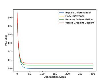
Figure 1: The MSE in Generalized Stackelberg’s model. Our method converges significantly faster than all the alternatives, and is the only method that do not fall into local minima.

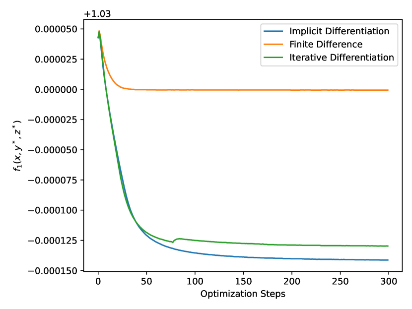
(a) Red wine quality dataset

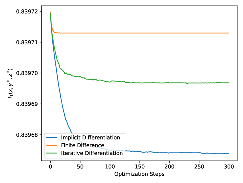
(b) White wine quality dataset

Figure 2: In the task of hyperparameter optimization, both the FD method and the ITD approach tend to converge to local minima.

Hyperparameter optimization

Table 1: Ratio of computational time relative to the vanilla method in Hyperparameter Optimization. This clearly demonstrates the efficiency of our method compared to Sato et al. [29].

Algorithm	VGD	FD	ITD	ID (ours)
Time per update	1	2.0	10.3	3.1

We evaluated these methods on regression tasks using the red and white wine quality datasets, as described in Cortez et al. [4], adopting the approach outlined in Sato et al. [29]. Each feature and target within the datasets was normalized prior to analysis. The outcomes of this evaluation are presented in Figure 2. We omitted the VGD method from our testing because the loss function $f_{1}$ does not explicitly include $\lambda$. Unlike other optimization algorithms that tend to get trapped in local minima, our method exhibits consistent improvement across iterations, surpassing the performance of the baseline methods. Additionally, the ratio of computational time relative to the vanilla method is presented in Table 1.

6 Related Work

A majority of work in this field tackle on the simplified bilevel cases. Our work draw inspiration from Gould et al. [12], which belongs to the school of first-order methods. Since then, more modern techniques have been proposed with stochastic nature as momentum recursive [5, 33] or variance reduction [25, 18] for optimizing computational complexity. Inspired by the technique leveraged in solving bilevel optimization problems, a wide array of machine learning applications flourish, such as hyperparameter optimization [1, 9, 22], reinforcement learning [17, 27, 15], neural architecture search [19, 35], meta-learning [8, 10, 26], and so on. Yet these works still leave a lot of room for improvement. For example, Liu et al. [19] leverages finite difference for neural architecture search, which is in essence a zero-order optimization method not utilizing the information to its full.

Recently more attempts have been made towards trilevel or multilevel problems [32, 30]. Inspired by the success of iterative differentiation in bilevel optimization, Sato et al. [29] proposed an approximate gradient-based method with theoretical guarantee. Nevertheless, the convergence analysis only holds asymptotically, hence requiring a considerably large iteration number in lower level, making it unsuitable for practical applications. There have also been efforts on the engineering side [13, 2]. Blondel et al. [2] proposed a modular framework for implicit differentiation, but failed to support multilevel optimization due to override of JAX’s automatic differentiation, which integrates the chain rule. Choe et al. [3] developed a software library for efficient automatic differentiation of multilevel optimization, but differs from our focus in that we propose the method for composing best-response Jacobian, which serves as the premise of their work.

7 Conclusion

Summary

In this study, we introduce an automatic differentiation method tailored for the gradient computation of trilevel optimization problems. We also develope a recursive algorithm designed for differentiation in general multilevel optimization scenarios, providing theoretical insights into the convergence rates applicable to both trilevel configurations and broader $n$-level contexts. Through comprehensive testing, our approach has been demonstrated to outperform existing methods significantly.

Limitations and Future Directions

The effectiveness of our algorithm is most evident within simpler systems and when handling a smaller number of levels $n$. While it yields relatively precise gradients for smooth and convex objective functions, challenges arise in optimizing non-convex functions, potentially leading to non-invertible Hessian matrices. Moreover, the efficiency of our gradient computation diminishes as the number of levels $n$ and the dimensionality of the features $d$ increase, due to the computational complexity scaling at $\mathcal{O}(d^{3}n^{4})$. Identifying heuristic methods to approximate gradients more efficiently remains for future exploration.

Appendix A Theoretical Proofs

The proof of lemma 2.1: Let $f:\mathbb{R}^{m+n}\to\mathbb{R}$ be a continuous function with second derivatives and $\det(\frac{\partial^{2}f}{\partial\bf{y}^{2}})\neq 0$. Let $\bf{g}(\bf{x})=\operatorname*{arg\,min}_{\bf y}f(\bf x,\bf y)$. Then the derivative of $\bf g$ with respect to $\bf x$ is

$$\dfrac{\mathop{}\!\mathrm{d}\mathbf{g}(\mathbf{x})}{\mathop{}\!\mathrm{d}\mathbf{x}}=-f_{YY}(\mathbf{x},\mathbf{g}(\mathbf{x}))^{-1}f_{XY}(\mathbf{x},\mathbf{g}(\mathbf{x}))$$

Proof.

First, since $\mathbf{g}(\mathbf{x})$ minimizes $f$ with respect to $\mathbf{y}$, the first order condition gives:

$$\frac{\partial f}{\partial\mathbf{y}}(\mathbf{x},\mathbf{g}(\mathbf{x}))=0.$$

Differentiating this condition with respect to $\mathbf{x}$ and applying the chain rule, we obtain:

$$\frac{\mathrm{d}}{\mathrm{d}\mathbf{x}}\left(\frac{\partial f}{\partial\mathbf{y}}(\mathbf{x},\mathbf{g}(\mathbf{x}))\right)=0.$$

This differentiation can be expanded as:

$$\frac{\partial^{2}f}{\partial\mathbf{x}\partial\mathbf{y}}+\frac{\partial^{2}f}{\partial\mathbf{y}^{2}}\frac{\mathrm{d}\mathbf{g}}{\mathrm{d}\mathbf{x}}=0.$$

Here, $\frac{\partial^{2}f}{\partial\mathbf{x}\partial\mathbf{y}}$ represents the matrix of mixed second partial derivatives of $f$ with respect to $\mathbf{x}$ and $\mathbf{y}$, and $\frac{\partial^{2}f}{\partial\mathbf{y}^{2}}$ is the Hessian matrix of $f$ with respect to $\mathbf{y}$.

To solve for $\frac{\mathrm{d}\mathbf{g}}{\mathrm{d}\mathbf{x}}$, rearrange the above equation:

$$\frac{\partial^{2}f}{\partial\mathbf{y}^{2}}\frac{\mathrm{d}\mathbf{g}}{\mathrm{d}\mathbf{x}}=-\frac{\partial^{2}f}{\partial\mathbf{x}\partial\mathbf{y}}.$$

Assuming $\frac{\partial^{2}f}{\partial\mathbf{y}^{2}}$ is invertible (as implied by $\det\left(\frac{\partial^{2}f}{\partial\mathbf{y}^{2}}\right)\neq 0$), we multiply both sides by the inverse of this matrix:

$$\frac{\mathrm{d}\mathbf{g}}{\mathrm{d}\mathbf{x}}=-\left(\frac{\partial^{2}f}{\partial\mathbf{y}^{2}}\right)^{-1}\frac{\partial^{2}f}{\partial\mathbf{x}\partial\mathbf{y}}$$

This completes the proof. ∎

The proof of lemma 3.1:

Let $f:\mathbb{R}^{d_{1}+d_{2}+d_{3}}\to\mathbb{R}$ be a continuous function with second derivatives. Let $\mathbf{g(x,y)}=\operatorname*{arg\,min}_{\mathbf{z}\in\mathbb{R}^{d_{3}}}f(\mathbf{x,y,z})$, then the following properties about $g$ holds:
(a)

$$\dfrac{\partial\mathbf{g}}{\partial\mathbf{x}}=-f_{ZZ}^{-1}f_{XZ}$$

(b)

$$\dfrac{\partial\mathbf{g}}{\partial\mathbf{y}}=-f_{ZZ}^{-1}f_{YZ}$$

Proof.

To find $\frac{\partial\mathbf{g}}{\partial\mathbf{x}}$, differentiate the first order condition with respect to $\mathbf{x}$ using the chain rule:

$$\frac{\mathrm{d}}{\mathrm{d}\mathbf{x}}\left(\frac{\partial f}{\partial\mathbf{z}}(\mathbf{x,y,g(x,y)})\right)=0.$$

Expanding this using the chain rule yields:

$$\frac{\partial^{2}f}{\partial\mathbf{x}\partial\mathbf{z}}+\frac{\partial^{2}f}{\partial\mathbf{z}^{2}}\frac{\partial\mathbf{g}}{\partial\mathbf{x}}=0.$$

Solving for $\frac{\partial\mathbf{g}}{\partial\mathbf{x}}$:

$$\frac{\partial\mathbf{g}}{\partial\mathbf{x}}=-\left(\frac{\partial^{2}f}{\partial\mathbf{z}^{2}}\right)^{-1}\frac{\partial^{2}f}{\partial\mathbf{x}\partial\mathbf{z}}.$$

The proof for part (b) is similar. ∎

The proof of lemma 3.2:

Let $f:\mathbb{R}^{d_{1}+d_{2}+d_{3}}\to\mathbb{R}$ and $\mathbf{g}:\mathbb{R}^{d_{1}+d_{2}}\to\mathbb{R}^{d_{3}}$ be continuous functions with second derivatives. Let $\mathbf{h(x)}=\operatorname*{arg\,min}_{y\in\mathbb{R}}f(\mathbf{x,y,g(x,y)})$, then the derivative of $\bf h$ with respect to $\bf x$ is:

$$\dfrac{\partial\mathbf{h}}{\partial\mathbf{x}}=-\left(f_{YY}+2f_{ZY}\dfrac{\partial\mathbf{g}}{\partial\mathbf{y}}+(\dfrac{\partial\mathbf{g}}{\partial\mathbf{y}})^{\top}f_{ZZ}\dfrac{\partial\mathbf{g}}{\partial\mathbf{y}}+\sum_{i=1}^{d_{3}}(f_{Z})_{i}\dfrac{\partial}{\partial\mathbf{y}}(\dfrac{\partial\mathbf{g}}{\partial\mathbf{y}})_{i}\right)^{-1}\\ \left(f_{XY}+f_{ZY}\dfrac{\partial\mathbf{g}}{\partial\mathbf{x}}+(\dfrac{\partial\mathbf{g}}{\partial\mathbf{y}})^{\top}f_{XZ}+(\dfrac{\partial\mathbf{g}}{\partial\mathbf{y}})^{\top}f_{ZZ}\dfrac{\partial\mathbf{g}}{\partial\mathbf{x}}+\sum_{i=1}^{d_{3}}(f_{Z})_{i}\dfrac{\partial}{\partial\mathbf{x}}(\dfrac{\partial\mathbf{g}}{\partial\mathbf{y}})_{i}\right)$$

Proof.

First, we establish the condition for $\mathbf{h}(\mathbf{x})$ by setting the gradient of $f$ with respect to $\mathbf{y}$ equal to zero, considering the implicit function defined by $\mathbf{g}$. The condition $\frac{\partial f}{\partial\mathbf{y}}+\frac{\partial f}{\partial\mathbf{z}}\frac{\partial\mathbf{g}}{\partial\mathbf{y}}=0$ must hold at the minimizer $\mathbf{y}=\mathbf{h}(\mathbf{x})$.

Differentiating this condition with respect to $\mathbf{x}$ gives:

$$\frac{\mathrm{d}}{\mathrm{d}\mathbf{x}}\left(\frac{\partial f}{\partial\mathbf{y}}+\frac{\partial f}{\partial\mathbf{z}}\frac{\partial\mathbf{g}}{\partial\mathbf{y}}\right)=0.$$

Expanding this derivative using the product and chain rules, we obtain:

$$f_{XY}+f_{YY}\frac{\partial\mathbf{h}}{\partial\mathbf{x}}+f_{YZ}\left(\frac{\partial\mathbf{g}}{\partial\mathbf{x}}+\frac{\partial\mathbf{g}}{\partial\mathbf{y}}\frac{\partial\mathbf{h}}{\partial\mathbf{x}}\right)+\\ \frac{\partial\mathbf{g}}{\partial\mathbf{y}}\left(f_{XY}+f_{YZ}\frac{\partial\mathbf{h}}{\partial\mathbf{x}}+f_{ZZ}\left(\frac{\partial\mathbf{g}}{\partial\mathbf{x}}+\frac{\partial\mathbf{g}}{\partial\mathbf{y}}\frac{\partial\mathbf{h}}{\partial\mathbf{x}}\right)\right)+f_{Z}\left(\frac{\partial^{2}\mathbf{g}}{\partial\mathbf{x}\partial\mathbf{y}}+\frac{\partial^{2}\mathbf{g}}{\partial\mathbf{y}^{2}}\frac{\partial\mathbf{h}}{\partial\mathbf{x}}\right)=0.$$

Rearranging terms and collecting like terms involving $\frac{\partial\mathbf{h}}{\partial\mathbf{x}}$, we find:

$$\left(f_{YY}+2f_{ZY}\dfrac{\partial\mathbf{g}}{\partial\mathbf{y}}+(\dfrac{\partial\mathbf{g}}{\partial\mathbf{y}})^{\top}f_{ZZ}\dfrac{\partial\mathbf{g}}{\partial\mathbf{y}}+\sum_{i=1}^{d_{3}}(f_{Z})_{i}\dfrac{\partial}{\partial\mathbf{y}}(\dfrac{\partial\mathbf{g}}{\partial\mathbf{y}})_{i}\right)\frac{\partial\mathbf{h}}{\partial\mathbf{x}}\\ =-\left(f_{XY}+f_{ZY}\dfrac{\partial\mathbf{g}}{\partial\mathbf{x}}+(\dfrac{\partial\mathbf{g}}{\partial\mathbf{y}})^{\top}f_{XZ}+(\dfrac{\partial\mathbf{g}}{\partial\mathbf{y}})^{\top}f_{ZZ}\dfrac{\partial\mathbf{g}}{\partial\mathbf{x}}+\sum_{i=1}^{d_{3}}(f_{Z})_{i}\dfrac{\partial}{\partial\mathbf{x}}(\dfrac{\partial\mathbf{g}}{\partial\mathbf{y}})_{i}\right)$$

Inverting the matrix on the left-hand side to solve for $\frac{\partial\mathbf{h}}{\partial\mathbf{x}}$, we obtain:

$$\dfrac{\partial\mathbf{h}}{\partial\mathbf{x}}=-\left(f_{YY}+2f_{ZY}\dfrac{\partial\mathbf{g}}{\partial\mathbf{y}}+(\dfrac{\partial\mathbf{g}}{\partial\mathbf{y}})^{\top}f_{ZZ}\dfrac{\partial\mathbf{g}}{\partial\mathbf{y}}+\sum_{i=1}^{d_{3}}(f_{Z})_{i}\dfrac{\partial}{\partial\mathbf{y}}(\dfrac{\partial\mathbf{g}}{\partial\mathbf{y}})_{i}\right)^{-1}\\ \left(f_{XY}+f_{ZY}\dfrac{\partial\mathbf{g}}{\partial\mathbf{x}}+(\dfrac{\partial\mathbf{g}}{\partial\mathbf{y}})^{\top}f_{XZ}+(\dfrac{\partial\mathbf{g}}{\partial\mathbf{y}})^{\top}f_{ZZ}\dfrac{\partial\mathbf{g}}{\partial\mathbf{x}}+\sum_{i=1}^{d_{3}}(f_{Z})_{i}\dfrac{\partial}{\partial\mathbf{x}}(\dfrac{\partial\mathbf{g}}{\partial\mathbf{y}})_{i}\right)$$

This expression for $\frac{\partial\mathbf{h}}{\partial\mathbf{x}}$ effectively describes how the minimizer $\mathbf{h}(\mathbf{x})$ changes as a function of $\mathbf{x}$. The matrix inversion reflects the dependency of the minimization outcome on the curvature of $f$ with respect to $\mathbf{y}$ and the interactions between $f$ and $\mathbf{g}$ via their cross-derivatives. The derivative $\frac{\partial\mathbf{h}}{\partial\mathbf{x}}$ encapsulates the net effect of these interactions and the underlying geometry of the function $f$ as modified by the mapping $\mathbf{g}$. ∎

The proof of theorem 4.1: Assume that $f_{i}$ for multilevel optimization is continuous with $i$-th order derivatives. If the second-order derivative of $f_{1}(\mathbf{x}_{1},\mathbf{x}_{2},\cdots,\mathbf{x}_{n})$ with respect to $\mathbf{x}_{1}$, i.e. the Hessian matrix $\frac{\mathop{}\!\mathrm{d}^{2}f_{1}}{\mathop{}\!\mathrm{d}\mathbf{x}_{1}^{2}}$, is positive definite and the maximum eigenvalue over every $\mathbf{x}_{1}$ is bounded, then we have

$$\mathbb{E}\big{(}\dfrac{\mathop{}\!\mathrm{d}f_{1}}{\mathop{}\!\mathrm{d}\mathbf{x}_{1}}\big{)}^{2}\leq\mathcal{O}\big{(}\frac{1}{N}\big{)}$$

Proof.

The basic proof approach is to compute the difference of $f_{1}$ value between two steps using Lagrange Mean Value Theorem and note that $f_{1}$ is actually a function of $\mathbf{x}_{1}$ because other variables $\mathbf{x}_{2},\cdots,\mathbf{x}_{n}$ are actually functions of $\mathbf{x}_{1}$. For simplicity, we use $\mathbf{x}^{i}$ to represent $\mathbf{x}^{i}(\mathbf{x}_{1}^{i})=(\mathbf{x}_{1}^{i},\mathbf{x}_{2}^{i}(\mathbf{x}_{1}^{i}),\cdots,\mathbf{x}_{n}^{i}(\mathbf{x}_{1}^{i},\cdots,\mathbf{x}_{n-1}^{i}))$ , where $\mathbf{x}_{2}^{i},\cdots,\mathbf{x}_{n}^{i}$ are optimal value as discussed in the $i$-th round. Then the difference will be

$$f_{1}(\mathbf{x}^{i+1})-f_{1}(\mathbf{x}^{i})$$

$$= f_{1}\big{(}\mathbf{x}_{1}^{i+1},\cdots,\mathbf{x}_{n}^{i+1}(\mathbf{x}_{1}^{i+1},\cdots,\mathbf{x}_{n-1}^{i+1})\big{)}-f_{1}\big{(}\mathbf{x}_{1}^{i},\cdots,\mathbf{x}_{n}^{i}(\mathbf{x}_{1}^{i},\cdots,\mathbf{x}_{n-1}^{i})\big{)}$$

$$= \frac{\mathop{}\!\mathrm{d}f_{1}}{\mathop{}\!\mathrm{d}\mathbf{x}_{1}}(\mathbf{x}^{i})\cdot(\mathbf{x}_{1}^{i+1}-\mathbf{x}_{1}^{i})+\frac{1}{2}(\mathbf{x}_{1}^{i+1}-\mathbf{x}_{1}^{i})^{T}\frac{\mathop{}\!\mathrm{d}^{2}f_{1}}{\mathop{}\!\mathrm{d}\mathbf{x}_{1}^{2}}(\mathbf{\xi})(\mathbf{x}_{1}^{i+1}-\mathbf{x}_{1}^{i})$$

where $\mathbf{\xi}$ is some value between $\mathbf{x}^{i}$ and $\mathbf{x}^{i+1}$ according to Lagrange Mean Value Theorem.

The Hessian matrix $\dfrac{\mathop{}\!\mathrm{d}^{2}f_{1}}{\mathop{}\!\mathrm{d}\mathbf{x}_{1}^{2}}$ is positive definite, so we have

$$(\mathbf{x}_{1}^{i+1}-\mathbf{x}_{1}^{i})^{T}\frac{\mathop{}\!\mathrm{d}^{2}f_{1}}{\mathop{}\!\mathrm{d}\mathbf{x}_{1}^{2}}(\mathbf{\xi})(\mathbf{x}_{1}^{i+1}-\mathbf{x}_{1}^{i}) \leq\lambda_{max}(\mathbf{x}_{1}^{i+1}-\mathbf{x}_{1}^{i})^{T}(\mathbf{x}_{1}^{i+1}-\mathbf{x}_{1}^{i})$$

$$=\lambda_{max}(\mathbf{x}_{1}^{i+1}-\mathbf{x}_{1}^{i})^{2}$$

where $\lambda_{max}$ is a bound of maximum eigenvalue over every $\mathbf{x}_{1}$ of the matrix $\dfrac{\mathop{}\!\mathrm{d}^{2}f_{1}}{\mathop{}\!\mathrm{d}\mathbf{x}_{1}^{2}}$, i.e.

$$\lambda\big{(}\dfrac{\mathop{}\!\mathrm{d}^{2}f_{1}}{\mathop{}\!\mathrm{d}\mathbf{x}_{1}^{2}}(\mathbf{x}(\mathbf{x}_{1},\cdots,\mathbf{x}_{n}))\big{)}\leq\lambda_{max}\ \forall\mathbf{x}_{1}$$

Note that we update $\mathbf{x}_{1}$ by

$$\mathbf{x}_{1}\leftarrow\mathbf{x}_{1}-\beta\frac{\mathop{}\!\mathrm{d}f_{1}}{\mathop{}\!\mathrm{d}\mathbf{x}_{1}}(\mathbf{x}_{1},\mathbf{x}_{2},\cdots,\mathbf{x}_{n})$$

we can replace $\mathbf{x}^{i+1}-\mathbf{x}^{i}$:

$$f_{1}(\mathbf{x}^{i+1})-f_{1}(\mathbf{x}^{i})$$

$$= \frac{\mathop{}\!\mathrm{d}f_{1}}{\mathop{}\!\mathrm{d}\mathbf{x}_{1}}(\mathbf{x}^{i})\cdot(\mathbf{x}_{1}^{i+1}-\mathbf{x}_{1}^{i})+\frac{1}{2}(\mathbf{x}_{1}^{i+1}-\mathbf{x}_{1}^{i})^{T}\frac{\mathop{}\!\mathrm{d}^{2}f_{1}}{\mathop{}\!\mathrm{d}\mathbf{x}_{1}^{2}}(\mathbf{\xi})(\mathbf{x}_{1}^{i+1}-\mathbf{x}_{1}^{i})$$

$$\leq \frac{\mathop{}\!\mathrm{d}f_{1}}{\mathop{}\!\mathrm{d}\mathbf{x}_{1}}(\mathbf{x}^{i})\cdot(\mathbf{x}_{1}^{i+1}-\mathbf{x}_{1}^{i})+\frac{1}{2}\lambda_{max}(\mathbf{x}_{1}^{i+1}-\mathbf{x}_{1}^{i})^{2}$$

$$= -\beta\big{(}\frac{\mathop{}\!\mathrm{d}f_{1}}{\mathop{}\!\mathrm{d}\mathbf{x}_{1}}(\mathbf{x}^{i})\big{)}^{2}+\frac{1}{2}\lambda_{max}\beta^{2}\big{(}\frac{\mathop{}\!\mathrm{d}f_{1}}{\mathop{}\!\mathrm{d}\mathbf{x}_{1}}(\mathbf{x}^{i})\big{)}^{2}$$

$$= \big{(}\frac{\lambda_{max}\beta^{2}}{2}-\beta\big{)}\big{(}\frac{\mathop{}\!\mathrm{d}f_{1}}{\mathop{}\!\mathrm{d}\mathbf{x}_{1}}(\mathbf{x}^{i})\big{)}^{2}$$

So we get

$$f_{1}(\mathbf{x}^{i+1})-f_{1}(\mathbf{x}^{i}) =f_{1}\big{(}\mathbf{x}_{1}^{i+1},\cdots,\mathbf{x}_{n}^{i+1}(\mathbf{x}_{1}^{i+1},\cdots,\mathbf{x}_{n-1}^{i+1})\big{)}-f_{1}\big{(}\mathbf{x}_{1}^{i},\cdots,\mathbf{x}_{n}^{i}(\mathbf{x}_{1}^{i},\cdots,\mathbf{x}_{n-1}^{i})\big{)}$$

$$\leq\big{(}\frac{\lambda_{max}\beta^{2}}{2}-\beta\big{)}\big{(}\frac{\mathop{}\!\mathrm{d}f_{1}}{\mathop{}\!\mathrm{d}\mathbf{x}_{1}}(\mathbf{x}^{i})\big{)}^{2}$$

After summing both sides, we find that the sum of the squared derivatives for each step can be bounded by a constant which is related to the initial point we select:

$$\big{(}\beta-\frac{\beta^{2}\lambda_{max}}{2}\big{)}\sum_{i=0}^{N-1}\big{(}\frac{\mathop{}\!\mathrm{d}f_{1}}{\mathop{}\!\mathrm{d}\mathbf{x}_{1}}(\mathbf{x}^{i})\big{)}^{2}$$

$$\leq f_{1}(\mathbf{x}^{0})-f_{1}(\mathbf{x}^{N})$$

$$\leq f_{1}(\mathbf{x}^{0})$$

So when $\beta\leq\frac{2}{\lambda_{max}}$, the expectation of the squared derivative can be approximated as

$$\mathbb{E}(\dfrac{\mathop{}\!\mathrm{d}f_{1}}{\mathop{}\!\mathrm{d}\mathbf{x}_{1}})^{2}\sim\dfrac{1}{N}\sum_{i=0}^{N-1}\big{(}\dfrac{\mathop{}\!\mathrm{d}f_{1}}{\mathop{}\!\mathrm{d}\mathbf{x}_{1}}\big{(}\mathbf{x}^{i})\big{)}^{2}\leq\dfrac{1}{N}\big{(}\beta-\frac{\beta^{2}\lambda_{max}}{2}\big{)}^{-1}f_{1}(\mathbf{x}_{0})=\mathcal{O}(\frac{1}{N})$$

by Central Limit Theorem. ∎

The proof of theorem 4.2:

Assume that $f_{i}$ are analytic functions satisfying

1. $|\frac{\partial f_{1}}{\partial x_{i}}|\leq N$ for all $x_{i}$.

2. $|\frac{\partial^{2}f_{1}}{\partial x_{i}^{2}}|\leq M$ for all $x_{i}$.

3. $|\frac{\partial x_{i}}{\partial x_{j}}|\leq K$ for all $j<i$.

4. $|\frac{\partial^{2}x_{i}}{\partial x_{j}^{2}}|\leq S$ for all $j<i$.

we have

$$\mathbb{E}(\dfrac{\mathop{}\!\mathrm{d}f_{1}}{\mathop{}\!\mathrm{d}x_{1}})^{2}\leq\dfrac{F_{0}(\beta-\frac{C\beta^{2}n^{n}J^{n+1}}{2})^{-1}}{N}\sim\mathcal{O}\big{(}\frac{n^{n}J^{n+1}}{N}\big{)}$$

Here $F_{0}$ is the value of $f_{1}$ at the initial point, $J$ is $\max\{M,N,K,S,1\}$, $\beta$ is the step size when we update $x_{1}$, $n$ is the number of layers, $N$ is the running rounds, and $C$ is a constant. And $x_{2},x_{3},\cdots,x_{n}$ are determined by the following system of equations:

$$\begin{cases}&x_{n}^{\star}=x_{n}(x_{1},\cdots,x_{n-1})=\arg\min_{x_{n}}f_{n}(x_{1},\cdots,x_{n})\\ &x_{n-1}^{\star}=x_{n-1}(x_{1},\cdots,x_{n-2})=\arg\min_{x_{n-1}}f_{n-1}(x_{1},\cdots,x_{n}^{\star})\\ &\vdots\\ &x_{3}^{\star}=x_{3}(x_{1},x_{2})=\arg\min_{x_{3}}f_{3}(x_{1},\cdots,x_{n}^{*})\\ &x_{2}^{\star}=x_{2}(x_{1})=\arg\min_{x_{2}}f_{2}(x_{1},x_{2},x_{3}^{\star}\cdots,x_{n}^{\star})\end{cases}$$

The $\frac{\partial x_{i}}{\partial x_{j}}$ and $\frac{\partial^{2}x_{i}}{\partial x_{j}^{2}}$ can be obtained like what we do in lemma 3.1 and lemma 3.2.

We begin with several lemmas:

Lemma A.1.

When assumption 3 holds, we have

$$|\dfrac{\mathop{}\!\mathrm{d}x_{i}}{\mathop{}\!\mathrm{d}x_{1}}(x)|\leq\mathcal{O}(((i-1)J)^{i-1})$$

for any $x$.

Proof.

Firstly, we have

$$|\dfrac{\mathop{}\!\mathrm{d}x_{2}}{\mathop{}\!\mathrm{d}x_{1}}(x)|=|\dfrac{\partial x_{2}}{\partial x_{1}}(x)|\leq K=\mathcal{O}(J)$$

Assume that

$$|\dfrac{\mathop{}\!\mathrm{d}x_{n}}{\mathop{}\!\mathrm{d}x_{1}}(x)|\leq\mathcal{O}(((n-1)J)^{n-1})$$

Then

$$|\dfrac{\mathop{}\!\mathrm{d}x_{n+1}}{\mathop{}\!\mathrm{d}x_{1}}(x)| =|\sum\limits_{j<n+1}\frac{\partial x_{n+1}}{\partial x_{j}}\cdot\frac{\mathop{}\!\mathrm{d}x_{j}}{\mathop{}\!\mathrm{d}x_{1}}(x)|$$

$$\leq\sum\limits_{j<n+1}|\frac{\partial x_{n+1}}{\partial x_{j}}(x)|\cdot|\frac{\mathop{}\!\mathrm{d}x_{j}}{\mathop{}\!\mathrm{d}x_{1}}(x)|$$

$$\leq\sum\limits_{j<n+1}K\mathcal{O}(((j-1)J)^{j-1})$$

$$\leq Kn\mathcal{O}(((n-1)J)^{n-1})$$

$$=\mathcal{O}((nJ)^{n})$$

By mathematical induction, we can get the conclusion

$$|\dfrac{\mathop{}\!\mathrm{d}x_{i}}{\mathop{}\!\mathrm{d}x_{1}}(x)|\leq\mathcal{O}(((i-1)J)^{i-1})$$

∎

Lemma A.2.

When assumption 3 and 4 hold, we have

$$|\dfrac{\mathop{}\!\mathrm{d}x_{i}}{\mathop{}\!\mathrm{d}x_{1}}(y)-\dfrac{\mathop{}\!\mathrm{d}x_{i}}{\mathop{}\!\mathrm{d}x_{1}}(z)|\leq\mathcal{O}(((i-1)J)^{i-1}S)|y-z|$$

for any $y$ and $z$.

Proof.

Firstly, we can get

$$|\dfrac{\mathop{}\!\mathrm{d}x_{2}}{\mathop{}\!\mathrm{d}x_{1}}(y)-\dfrac{\mathop{}\!\mathrm{d}x_{2}}{\mathop{}\!\mathrm{d}x_{1}}(z)|\leq S|y-z|=\mathcal{O}(JS)|y-z|$$

easily from the assumption 4.

Assume that

$$|\dfrac{\mathop{}\!\mathrm{d}x_{n}}{\mathop{}\!\mathrm{d}x_{1}}(y)-\dfrac{\mathop{}\!\mathrm{d}x_{n}}{\mathop{}\!\mathrm{d}x_{1}}(z)|\leq\mathcal{O}(((n-1)J)^{n-1}S)|y-z|$$

Then

$$|\dfrac{\mathop{}\!\mathrm{d}x_{n+1}}{\mathop{}\!\mathrm{d}x_{1}}(y)-\dfrac{\mathop{}\!\mathrm{d}x_{n+1}}{\mathop{}\!\mathrm{d}x_{1}}(z)| =|\sum\limits_{j<n+1}\frac{\partial x_{n+1}}{\partial x_{j}}\cdot\frac{\mathop{}\!\mathrm{d}x_{j}}{\mathop{}\!\mathrm{d}x_{1}}(y)-\sum\limits_{j<n+1}\frac{\partial x_{n+1}}{\partial x_{j}}\cdot\frac{\mathop{}\!\mathrm{d}x_{j}}{\mathop{}\!\mathrm{d}x_{1}}(z)|$$

$$\leq\sum\limits_{j<n+1}|\frac{\partial x_{n+1}}{\partial x_{j}}\cdot\frac{\mathop{}\!\mathrm{d}x_{j}}{\mathop{}\!\mathrm{d}x_{1}}(y)-\frac{\partial x_{n+1}}{\partial x_{j}}\cdot\frac{\mathop{}\!\mathrm{d}x_{j}}{\mathop{}\!\mathrm{d}x_{1}}(z)|$$

$$\leq\sum\limits_{j<n+1}(|\frac{\partial x_{n+1}}{\partial x_{j}}(y)\frac{\mathop{}\!\mathrm{d}x_{j}}{\mathop{}\!\mathrm{d}x_{1}}(y)-\frac{\partial x_{n+1}}{\partial x_{j}}(y)\frac{\mathop{}\!\mathrm{d}x_{j}}{\mathop{}\!\mathrm{d}x_{1}}(z)|$$

$$\ \ \ \ \ \ \ \ \ \ \ \ \ \ \ \ +|\frac{\partial x_{n+1}}{\partial x_{j}}(y)\frac{\mathop{}\!\mathrm{d}x_{j}}{\mathop{}\!\mathrm{d}x_{1}}(z)-\frac{\partial x_{n+1}}{\partial x_{j}}(z)\frac{\mathop{}\!\mathrm{d}x_{j}}{\mathop{}\!\mathrm{d}x_{1}}(z)|)$$

$$\leq\sum\limits_{j<n+1}(K\mathcal{O}(((j-1)J)^{j-1}S)|y-z|$$

$$\ \ \ \ \ \ \ \ \ \ \ \ \ \ \ \ +S|y-z|\mathcal{O}(((j-1)J)^{j-1}))$$

$$\leq n(K\mathcal{O}(((n-1)J)^{n-1}S)+S\mathcal{O}(((n-1)J)^{n-1}))|y-z|$$

$$=\mathcal{O}((nJ)^{n}S)|y-z|$$

By mathematical induction, we can get the conclusion

$$|\dfrac{\mathop{}\!\mathrm{d}x_{i}}{\mathop{}\!\mathrm{d}x_{1}}(y)-\dfrac{\mathop{}\!\mathrm{d}x_{i}}{\mathop{}\!\mathrm{d}x_{1}}(z)|\leq\mathcal{O}(((i-1)J)^{i-1}S)|y-z|$$

∎

Lemma A.3.

When assumption 1-4 hold, we have

$$|\dfrac{\mathop{}\!\mathrm{d}f_{1}}{\mathop{}\!\mathrm{d}x_{1}}(y)-\dfrac{\mathop{}\!\mathrm{d}f_{1}}{\mathop{}\!\mathrm{d}x_{1}}(z)|\leq\mathcal{O}(n^{n}J^{n-1}(SN+M))|y-z|=\mathcal{O}(n^{n}J^{n+1})|y-z|$$

for any $y$ and $z$.

Proof.

We can use the triangle inequality to unravel the difference:

$$|\dfrac{\mathop{}\!\mathrm{d}f_{1}}{\mathop{}\!\mathrm{d}x_{1}}(y)-\dfrac{\mathop{}\!\mathrm{d}f_{1}}{\mathop{}\!\mathrm{d}x_{1}}(z)| =|\sum\limits_{j=1}^{n}\frac{\partial f_{1}}{\partial x_{j}}\cdot\frac{\mathop{}\!\mathrm{d}x_{j}}{\mathop{}\!\mathrm{d}x_{1}}(y)-\sum\limits_{j=1}^{n}\frac{\partial f_{1}}{\partial x_{j}}\cdot\frac{\mathop{}\!\mathrm{d}x_{j}}{\mathop{}\!\mathrm{d}x_{1}}(z)|$$

$$\leq\sum\limits_{j=1}^{n}|\frac{\partial f_{1}}{\partial x_{j}}\cdot\frac{\mathop{}\!\mathrm{d}x_{j}}{\mathop{}\!\mathrm{d}x_{1}}(y)-\frac{\partial f_{1}}{\partial x_{j}}\cdot\frac{\mathop{}\!\mathrm{d}x_{j}}{\mathop{}\!\mathrm{d}x_{1}}(z)|$$

$$\leq\sum\limits_{j=1}^{n}(|\frac{\partial f_{1}}{\partial x_{j}}(y)\frac{\mathop{}\!\mathrm{d}x_{j}}{\mathop{}\!\mathrm{d}x_{1}}(y)-\frac{\partial f_{1}}{\partial x_{j}}(y)\frac{\mathop{}\!\mathrm{d}x_{j}}{\mathop{}\!\mathrm{d}x_{1}}(z)|$$

$$\ \ \ \ \ \ \ \ \ \ \ \ \ \ \ \ +|\frac{\partial f_{1}}{\partial x_{j}}(y)\frac{\mathop{}\!\mathrm{d}x_{j}}{\mathop{}\!\mathrm{d}x_{1}}(z)-\frac{\partial f_{1}}{\partial x_{j}}(z)\frac{\mathop{}\!\mathrm{d}x_{j}}{\mathop{}\!\mathrm{d}x_{1}}(z)|)$$

$$\leq\sum\limits_{j=1}^{n}(N\mathcal{O}(((j-1)J)^{j-1}S)|y-z|+M|y-z|\mathcal{O}(((j-1)J)^{j-1}))$$

$$\leq n(N\mathcal{O}(((n-1)J)^{n-1}S)+M\mathcal{O}(((n-1)J)^{n-1})))|y-z|$$

$$\leq\mathcal{O}(n^{n}J^{n-1}(SN+M))|y-z|$$

$$=\mathcal{O}(n^{n}J^{n+1})|y-z|$$

∎

According to the three lemmas, we can prove the general conclusion given above:

Theorem A.4.

When the functions $f_{i}\ (\forall i)$ in $n$-level optimization and $x_{j}\ (\forall j>1)$ derived from them can satisfy the assumptions 1-4, we will have

$$\mathbb{E}(\dfrac{\mathop{}\!\mathrm{d}f_{1}}{\mathop{}\!\mathrm{d}x_{1}})^{2}\leq\dfrac{F_{0}}{N}(\beta-\frac{C\beta^{2}n^{n}J^{n+1}}{2})^{-1}$$

Proof.

For simplicity, we use $x^{i}$ to represent $x^{i}(x_{1}^{i})=(x_{1}^{i},x_{2}^{i},\cdots,x_{n}^{i})$ in the $i$-th round, where $x_{2}^{i},\cdots,x_{n}^{i}$ are all functions of $x_{1}^{i}$, just like what is said in the system of equations LABEL:equations. From lemma A.3, we know that there is a constant C such that

$$|\dfrac{\mathop{}\!\mathrm{d}^{2}f_{1}}{\mathop{}\!\mathrm{d}x_{1}^{2}}|\leq Cn^{n}J^{n+1}$$

We can also compute the difference of $f_{1}$ between two rounds:

$$f_{1}(x^{i+1})-f_{1}(x^{i})$$

$$= \frac{\mathop{}\!\mathrm{d}f_{1}}{\mathop{}\!\mathrm{d}x_{1}}(x^{i})(x_{1}^{i+1}-x_{1}^{i})+\frac{1}{2}\dfrac{\mathop{}\!\mathrm{d}^{2}f_{1}}{\mathop{}\!\mathrm{d}x_{1}^{2}}(\xi^{i})(x_{1}^{i+1}-x_{1}^{i})^{2}$$

$$\leq -\beta(\frac{\mathop{}\!\mathrm{d}f_{1}}{\mathop{}\!\mathrm{d}x_{1}}(x^{i}))^{2}+\frac{1}{2}\beta^{2}(\frac{\mathop{}\!\mathrm{d}f_{1}}{\mathop{}\!\mathrm{d}x_{1}}(x^{i}))^{2}Cn^{n}J^{n+1}$$

Sum the both sides and when $\beta<\frac{2}{Cn^{n}J^{n+1}}$, we can get

$$\sum_{i=0}^{N-1}(\dfrac{\mathop{}\!\mathrm{d}f_{1}}{\mathop{}\!\mathrm{d}x_{1}}(x^{i}))^{2}$$

$$\leq (\beta-\frac{C\beta^{2}n^{n}J^{n+1}}{2})^{-1}(f_{1}(x^{0})-f_{1}(x^{N}))$$

$$\leq (\beta-\frac{C\beta^{2}n^{n}J^{n+1}}{2})^{-1}f_{1}(x^{0})$$

$$= F_{0}(\beta-\frac{C\beta^{2}n^{n}J^{n+1}}{2})^{-1}$$

By Central Limit Theorem, we have

$$\mathbb{E}(\dfrac{\mathop{}\!\mathrm{d}f_{1}}{\mathop{}\!\mathrm{d}x_{1}})^{2}\sim\frac{1}{N}\sum_{i=0}^{N-1}(\dfrac{\mathop{}\!\mathrm{d}f_{1}}{\mathop{}\!\mathrm{d}x_{1}}(x^{i}))^{2}\leq\dfrac{F_{0}}{N}(\beta-\frac{C\beta^{2}n^{n}J^{n+1}}{2})^{-1}$$

∎

From the above proof, note that:

1. These four assumptions about the boundedness of derivatives can also be replaced by the boundedness of the lipschitz constants for $f_{1}$ and $x_{j}\ (\forall j>1)$ and their corresponding derivatives.

2. In fact, $x_{j}\ (\forall j>1)$ depends on $f_{i}\ (\forall i>1)$. Due to the structure of $n$-level optimization, the various derivatives of $x_{j}$ can be bounded by the lipschitz constants of various derivatives of $f_{i}$, which may lead to more optimal bounds. In fact, the expectation of $(\dfrac{\mathop{}\!\mathrm{d}f_{1}}{\mathop{}\!\mathrm{d}x_{1}})^{2}$ can be bounded by the lipschitz constants of the each order derivative of $f_{i}\ (\forall i)$.

3. This bound is intuitive. Note that $\beta<\frac{2}{Cn^{n}J^{n+1}}$, so we can choose $\beta=\frac{1}{Cn^{n}J^{n+1}}$, it means

   $$\mathbb{E}(\dfrac{\mathop{}\!\mathrm{d}f_{1}}{\mathop{}\!\mathrm{d}x_{1}})^{2}\leq\dfrac{2Cn^{n}J^{n+1}F_{0}}{N}$$

   As the number of layers $n$ increases, more rounds $N$ is needed to update $x_{1}$ to achieve the convergence.

4. This theorem explains that in general, when the domain of $\mathbf{x}_{1}$ is not a compact convex set, the algorithm we use still converges, although it may not necessarily converge to the optimal value.

References

• Bennett et al. [2006] K. P. Bennett, J. Hu, X. Ji, G. Kunapuli, and J.-S. Pang. Model selection via bilevel optimization. In The 2006 IEEE International Joint Conference on Neural Network Proceedings, pages 1922–1929. IEEE, 2006.
• Blondel et al. [2022] M. Blondel, Q. Berthet, M. Cuturi, R. Frostig, S. Hoyer, F. Llinares-López, F. Pedregosa, and J.-P. Vert. Efficient and modular implicit differentiation. Advances in neural information processing systems, 35:5230–5242, 2022.
• Choe et al. [2022] S. K. Choe, W. Neiswanger, P. Xie, and E. Xing. Betty: An automatic differentiation library for multilevel optimization. arXiv preprint arXiv:2207.02849, 2022.
• Cortez et al. [2009] P. Cortez, A. Cerdeira, F. Almeida, T. Matos, and J. Reis. Modeling wine preferences by data mining from physicochemical properties. Decision support systems, 47(4):547–553, 2009.
• Cutkosky and Orabona [2019] A. Cutkosky and F. Orabona. Momentum-based variance reduction in non-convex sgd. Advances in neural information processing systems, 32, 2019.
• Dempe and Zemkoho [2020] S. Dempe and A. Zemkoho. Bilevel optimization. In Springer optimization and its applications, volume 161. Springer, 2020.
• Domke [2012] J. Domke. Generic methods for optimization-based modeling. In Artificial Intelligence and Statistics, pages 318–326. PMLR, 2012.
• Finn et al. [2017] C. Finn, P. Abbeel, and S. Levine. Model-agnostic meta-learning for fast adaptation of deep networks. In International conference on machine learning, pages 1126–1135. PMLR, 2017.
• Franceschi et al. [2017] L. Franceschi, M. Donini, P. Frasconi, and M. Pontil. Forward and reverse gradient-based hyperparameter optimization. In International Conference on Machine Learning, pages 1165–1173. PMLR, 2017.
• Franceschi et al. [2018a] L. Franceschi, P. Frasconi, S. Salzo, R. Grazzi, and M. Pontil. Bilevel programming for hyperparameter optimization and meta-learning. In International conference on machine learning, pages 1568–1577. PMLR, 2018a.
• Franceschi et al. [2018b] L. Franceschi, R. Grazzi, M. Pontil, S. Salzo, and P. Frasconi. Far-ho: A bilevel programming package for hyperparameter optimization and meta-learning. arXiv preprint arXiv:1806.04941, 2018b.
• Gould et al. [2016] S. Gould, B. Fernando, A. Cherian, P. Anderson, R. S. Cruz, and E. Guo. On differentiating parameterized argmin and argmax problems with application to bi-level optimization. arXiv preprint arXiv:1607.05447, 2016.
• Grefenstette et al. [2019] E. Grefenstette, B. Amos, D. Yarats, P. M. Htut, A. Molchanov, F. Meier, D. Kiela, K. Cho, and S. Chintala. Generalized inner loop meta-learning. arXiv preprint arXiv:1910.01727, 2019.
• Hestenes et al. [1952] M. R. Hestenes, E. Stiefel, et al. Methods of conjugate gradients for solving linear systems. NBS Washington, DC, 1952.
• Hong et al. [2023] M. Hong, H.-T. Wai, Z. Wang, and Z. Yang. A two-timescale stochastic algorithm framework for bilevel optimization: Complexity analysis and application to actor-critic. SIAM Journal on Optimization, 33(1):147–180, 2023.
• Kingma and Ba [2017] D. P. Kingma and J. Ba. Adam: A method for stochastic optimization, 2017.
• Konda and Tsitsiklis [1999] V. Konda and J. Tsitsiklis. Actor-critic algorithms. Advances in neural information processing systems, 12, 1999.
• Li and Li [2018] Z. Li and J. Li. A simple proximal stochastic gradient method for nonsmooth nonconvex optimization. Advances in neural information processing systems, 31, 2018.
• Liu et al. [2018] H. Liu, K. Simonyan, and Y. Yang. Darts: Differentiable architecture search. arXiv preprint arXiv:1806.09055, 2018.
• Liu et al. [2021] R. Liu, J. Gao, J. Zhang, D. Meng, and Z. Lin. Investigating bi-level optimization for learning and vision from a unified perspective: A survey and beyond. IEEE Transactions on Pattern Analysis and Machine Intelligence, 44(12):10045–10067, 2021.
• Liu et al. [2023] R. Liu, X. Liu, S. Zeng, J. Zhang, and Y. Zhang. Value-function-based sequential minimization for bi-level optimization. IEEE Transactions on Pattern Analysis and Machine Intelligence, 2023.
• Lorraine et al. [2020] J. Lorraine, P. Vicol, and D. Duvenaud. Optimizing millions of hyperparameters by implicit differentiation. In International conference on artificial intelligence and statistics, pages 1540–1552. PMLR, 2020.
• MacKay et al. [2019] M. MacKay, P. Vicol, J. Lorraine, D. Duvenaud, and R. Grosse. Self-tuning networks: Bilevel optimization of hyperparameters using structured best-response functions. arXiv preprint arXiv:1903.03088, 2019.
• Maclaurin et al. [2015] D. Maclaurin, D. Duvenaud, and R. Adams. Gradient-based hyperparameter optimization through reversible learning. In International conference on machine learning, pages 2113–2122. PMLR, 2015.
• Nguyen et al. [2017] L. M. Nguyen, J. Liu, K. Scheinberg, and M. Takáč. Sarah: A novel method for machine learning problems using stochastic recursive gradient. In International conference on machine learning, pages 2613–2621. PMLR, 2017.
• Rajeswaran et al. [2019] A. Rajeswaran, C. Finn, S. M. Kakade, and S. Levine. Meta-learning with implicit gradients. Advances in neural information processing systems, 32, 2019.
• Rajeswaran et al. [2020] A. Rajeswaran, I. Mordatch, and V. Kumar. A game theoretic framework for model based reinforcement learning. In International conference on machine learning, pages 7953–7963. PMLR, 2020.
• Samuel and Tappen [2009] K. G. Samuel and M. F. Tappen. Learning optimized map estimates in continuously-valued mrf models. In 2009 IEEE Conference on Computer Vision and Pattern Recognition, pages 477–484. IEEE, 2009.
• Sato et al. [2021] R. Sato, M. Tanaka, and A. Takeda. A gradient method for multilevel optimization. Advances in Neural Information Processing Systems, 34:7522–7533, 2021.
• Shafiei et al. [2021] A. Shafiei, V. Kungurtsev, and J. Marecek. Trilevel and multilevel optimization using monotone operator theory. arXiv preprint arXiv:2105.09407, 2021.
• Stackelberg and Peacock [1952] H. v. Stackelberg and A. T. Peacock. The theory of the market economy. (No Title), 1952.
• Tilahun et al. [2012] S. L. Tilahun, S. M. Kassa, and H. C. Ong. A new algorithm for multilevel optimization problems using evolutionary strategy, inspired by natural adaptation. In PRICAI 2012: Trends in Artificial Intelligence: 12th Pacific Rim International Conference on Artificial Intelligence, Kuching, Malaysia, September 3-7, 2012. Proceedings 12, pages 577–588. Springer, 2012.
• Tran-Dinh et al. [2019] Q. Tran-Dinh, N. H. Pham, D. T. Phan, and L. M. Nguyen. Hybrid stochastic gradient descent algorithms for stochastic nonconvex optimization. arXiv preprint arXiv:1905.05920, 2019.
• Yang et al. [2021] J. Yang, K. Ji, and Y. Liang. Provably faster algorithms for bilevel optimization. Advances in Neural Information Processing Systems, 34:13670–13682, 2021.
• Zhang et al. [2021] M. Zhang, S. W. Su, S. Pan, X. Chang, E. M. Abbasnejad, and R. Haffari. idarts: Differentiable architecture search with stochastic implicit gradients. In International Conference on Machine Learning, pages 12557–12566. PMLR, 2021.
• Zhang et al. [2024] Y. Zhang, P. Khanduri, I. Tsaknakis, Y. Yao, M. Hong, and S. Liu. An introduction to bilevel optimization: Foundations and applications in signal processing and machine learning. IEEE Signal Processing Magazine, 41(1):38–59, 2024.