TSDS: Data Selection for Task-Specific Model Finetuning
Abstract
Finetuning foundation models for specific tasks is an emerging paradigm in modern machine learning. The efficacy of task-specific finetuning largely depends on the selection of appropriate training data. We present TSDS (Task-Specific Data Selection), a framework to select data for task-specific model finetuning, guided by a small but representative set of examples from the target task. To do so, we formulate data selection for task-specific finetuning as an optimization problem with a distribution alignment loss based on optimal transport to capture the discrepancy between the selected data and the target distribution. In addition, we add a regularizer to encourage the diversity of the selected data and incorporate kernel density estimation into the regularizer to reduce the negative effects of near-duplicates among the candidate data. We connect our optimization problem to nearest neighbor search and design efficient algorithms to compute the optimal solution based on approximate nearest neighbor search techniques. We evaluate our method on data selection for both continued pretraining and instruction tuning of language models. We show that instruction tuning using data selected by our method with a 1% selection ratio often outperforms using the full dataset and beats the baseline selection methods by 1.5 points in F1 score on average. Our code is available at https://github.com/ZifanL/TSDS.
1 Introduction
Finetuning foundation models [3] is the de-facto paradigm for building machine learning applications that focus on specific tasks. Models such as BERT [10] and LLaMA [43] are large-scale models pretrained on massive unlabeled data across a wide range of domains. Those models can be specialized to downstream tasks through finetuning. Finetuning can take a variety of forms depending on the target task. For instance, continued pretraining [17] extends the pretraining stage of a model on a dataset that is more closely related to a target domain. As another setting, instruction tuning [51] trains a generative foundation model on instruction-response pairs to improve its performance in responding to task-specific instructions.
Finetuning foundation models can lead to significant improvement in downstream tasks, but the effectiveness heavily relies on the right choice of training data [17, 30, 48, 47]. However, the data repositories that one considers during training of generative models tend to be large—consider for example the use of Common Crawl111https://commoncrawl.org/, which contains 250 billion web pages, or The Pile [14]—and hence, it is impractical to manually select the data that are distributed like the use cases in the target task. Therefore, automated task-specific data selection becomes critical.
In this paper, we propose TSDS (Task-Specific Data Selection), a framework to select data for task-specific model finetuning. We consider the scenario of finetuning a foundation model to customize it for a specific task characterized by a few representative examples. The input to our framework is the representative examples and a massive repository of candidate data. Guided by the representative examples, we select training data from the repository for task-specific finetuning. We identify the following requirements for our framework.
(Distribution Alignment) First, the distribution of the selected data should match the distribution of the representative examples from the target task. Distribution alignment is essential for a model to learn the target distribution and enable data-efficient finetuning for the target task [40]. Many works [38, 17, 2, 50, 47] retrieve candidate examples that are most similar to the representative examples. Such heuristics do not ensure distribution alignment between the selected data and the representative examples. A recent work [48] selects data by importance resampling to match the target distribution but is limited to an n-gram feature space, which cannot capture high-level semantics.
(Diversity) Second, the selected data should be diverse so that the model can learn a wide range of related knowledge rather than overfitting to specific examples. In practice, data repositories created by web crawling may contain a large portion of near-duplicates [13, 28] that can compromise diversity and negatively impact model performance [28, 19]. For example, a study [13] on several snapshots of ClueWeb222https://lemurproject.org/ and Common Crawl shows that 14% to 52% of the documents are near-duplicates. Previous works [38, 17, 2, 50, 48, 47] on task-specific data selection overlook near-duplicates, leading to the over-representation of such examples in the selected data. We require our framework to ensure diversity in selection even when a large fraction of the candidate examples are near-duplicates.
(Scalability) Finally, the selection algorithm should be efficient, considering the increasing scale of modern data repositories. The high volume of candidate data (e.g., 250 billion pages in Common Crawl) poses a great challenge to efficient selection.
Our framework formulates task-specific data selection as an optimization problem that allows a smooth trade-off between two crucial objectives: distribution alignment and diversity. The solution to the optimization problem is a categorical distribution assigned to the candidates which we will sample from. In the optimization objective, we use optimal transport to measure the discrepancy between the distribution assigned to the candidates and the target distribution, encouraging the alignment between them. We show that the optimization problem admits efficient algorithms to compute the optimal solution. In addition, our framework supports distribution alignment in any metric space that supports efficient nearest-neighbor search, including model-agnostic semantic embedding and model-specific features such as gradients.
Our contributions: 1) We formulate data selection for task-specific finetuning as an optimization problem based on optimal transport for distribution alignment, with a regularization term that encourages diversity. 2) We make our framework robust to near-duplicates by incorporating kernel density estimation [36] into the regularization term. 3)We show the connection between the optimal solution to the optimization problem and nearest neighbor search, which allows us to develop efficient algorithms employing approximate nearest-neighbor search techniques [23].
We conduct extensive experiments to validate the effectiveness of our framework. We focus on natural language processing tasks where foundation models have shown great advancements. We show that our framework beats the state-of-the-art baseline [47] by points in F1 score on average with a selection ratio of 1% on instruction tuning for two modern large language models on three tasks. In addition, continued pretraining using domain-specific data selected by our framework outperforms the other selection methods by up to 3 F1 points on four classification tasks from various domains. We also demonstrate that our framework is robust to near-duplicates in the data repository, maintaining consistent performance when 1% of the candidate examples are duplicate for up to 1,000 times. Our method is efficient, taking 28 hours to preprocess a corpus of 150M examples and less than 1 hour for each task-specific selection.
2 Background and Overview
In this section, we provide background information that is essential for the problem, followed by a formal statement of the problem and an overview of our proposed framework.
2.1 Background
We introduce the notations that will be used throughout the paper and the optimal transport problem.
Notation We use to represent the set of non-negative real numbers, and to represent the set of positive real numbers. Let be a positive integer and we use to denote the set of integers from to . We use bold letters to denote matrices and the corresponding plain letters with subscripts to denote the entries in the matrix. For example, is a matrix with size , and or is the entry in the row and the column (-indexed).
Optimal Transport between Discrete Distributions We introduce the optimal transport problem, which forms the basis of our data selection framework. Let be a metric space where is a finite set and is a distance function. Consider two discrete distributions on and on , where both and are finite sets. Let be the example in and be the probability of . Similarly, let be the example in and be the probability of . Let be a transport of probability mass between and , where is amount of probability mass transported from to . Assume that the cost of transporting one unit of probability mass from to is , the distance between and . Optimal transport is the problem of transporting all the probability mass from to with a minimal cost:
2.2 Task-Specific Data Selection Problem Statement
We now introduce the problem of data selection for task-specific finetuning. We assume access to a set of representative examples from the target task, which we call query examples. Consider a data repository containing candidate examples. Note that and are multisets that may contain duplicates. We aim to select examples from the repository guided by the query examples. The selected examples will be used to finetune a model to tailor it to the target task. We adopt the model-agnostic formulation above for the generality of the solution. However, our framework can be applied to model-specific selection by using model-specific data representations; an example evaluation for model-specific instruction tuning is presented in Section 5.1.
2.3 Framework Overview
Our framework takes the candidate examples and the query examples as inputs and outputs a set of task-specific examples by the following workflow. 1. (Encoding) We first encode the query examples and the candidate examples into the same metric space with a specified distance function. 2. (Probability Assignment) We determine the probability mass assigned to each candidate example by solving an optimization problem. 3. (Sampling) We take a random sample with replacement from the candidate examples following a categorical distribution where the probability is determined by the assignment in the previous step.
3 Data Selection and Optimal Transport
Data selection for task-specific finetuning can be expressed as an optimization problem for probability assignment to the candidates in the data repository. First, we discuss the formulation of the optimization problem and then show the existence of closed-form solutions. In addition, we propose a regularization term that addresses the problem of near-duplicates among the candidates. The proofs of the theorems in this section are provided in Appendix B.
3.1 Optimization Problem
Consider the metric space where contains all the examples and is a distance function. Let be the distance matrix, where is the distance between the query example and the candidate example.
We propose an optimization problem that transports probability mass from the query examples to the candidates. The objective is a linear combination of a probability transport cost for distribution alignment and a regularization term to encourage diversity. Formally, given , we consider the following optimization problem, which we refer to as Problem RT (regularized transport):
where is a scaling constant, is a hyper-parameter that controls the trade-off between distribution alignment and diversity, and is a regularization function. The first term in Problem RT is the cost of probability transport where is the mass transported from the query example to the candidate. Each query example has probability mass to transport, as stated in the constraint. The probability transport cost measures the cost of transforming one distribution to another by moving probability mass between them, providing a method to quantify probability alignment. The second is a regularization term that encourages the diversity of probability transport.
Let be an optimal solution to Problem RT. We assign probability to candidate example , which is the sum of the probability mass it receives from all the query examples. When we sample from the candidate examples in the subsequent step, has probability .
We propose two instantiations of the regularization term that encourage the diversity of probability transport by penalizing its discrepancy to the uniform transport:
-
•
captures the largest probability gap between and the uniform transport.
-
•
is the total variation distance between and the uniform transport.
We use uniform transport as a reference point to encourage diversity as it represents the most diverse way of transporting the probability mass from one query example to all the candidates, assuming the candidates are distinct.
3.2 Closed-Form Solution
When , Problem RT can be solved by standard linear programming techniques, but they run in time, which is prohibitively expensive. Instead, we show the existence of a closed-form solution that can be computed in time (see Section 4 for the algorithm).
Using as the regularization function, we get an optimal solution by transporting the probability of each query example evenly to its -nearest neighbors among the candidates, where is determined by the tradeoff between distribution alignment and diversity:
Theorem 3.1.
Similarly, there exists a closed-form solution that can be computed in time when (see Appendix A for the solution and the algorithm).
3.3 Addressing Near-Duplicates via Kernel Density Estimation
When there exists a large fraction of near-duplicates among the candidates, fails to characterize the diversity of probability assignment since it treats near-duplicates as distinct examples. Consequently, the contents in the near-duplicates will be over-sampled. For example, if of the -nearest neighbors of a query example are duplicates and the others are distinct, the content in the duplicates will receive times as much probability mass as any other example.
To address the near-duplicate problem, we propose a regularization function incorporating kernel density estimation (KDE) [36], which is a non-parametric method to estimate the probability density function from finite examples. We determine the duplication level of a point by the kernel density estimate at its position. We use the Epanechnikov kernel such that given , the density estimate at point is , where is the kernel size and is the distance function. For example, for a point in whose distance to any other point is larger than , the density estimate at is . If we create two duplicates of and add them to , the density estimate at increases to .
Our KDE-based regularization function is where is the density estimate at . compares to the probability assignment that is proportional to the inverse of the density, and penalizes the largest gap weighted by the density. Note that is a special case of with for all .
The optimal solution to Problem RT when can be obtained by assigning the probability mass of each query example to the nearest neighbors among the candidates, weighted by the inverse of their density estimate, as is shown by the following theorem.
Theorem 3.2.
Intuitively, we count candidate as examples. For each query example, the optimal solution assigns probability mass to the candidates in its neighborhood proportional to their adjusted counts. The size of the neighborhood is determined by the limit on the sum of the adjusted counts.
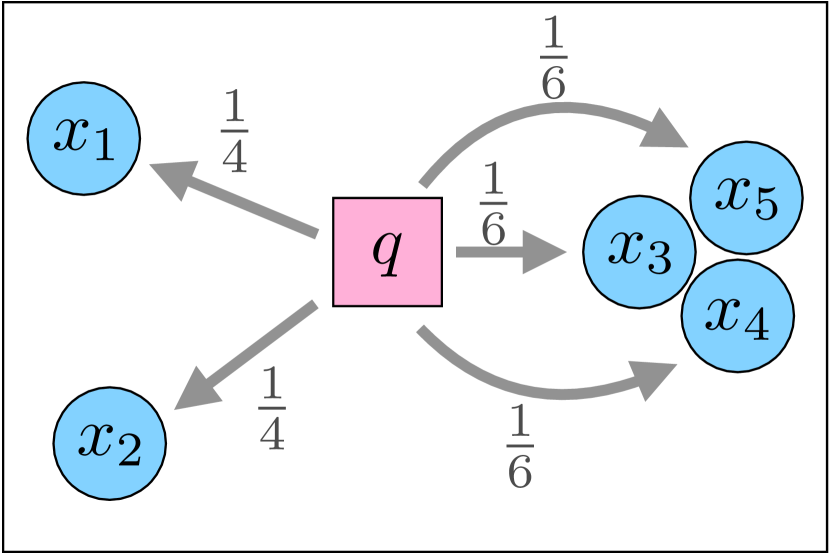
In Figure 1, we show an example comparing the optimal transport with and . When , the probability is transported uniformly to the candidates regardless of their relative positions. When , the clustered candidates receive less probability due to their high density, and they will be less over-represented when we take samples according to the assigned probability.

4 Efficient Probability Assignment Algorithms for Data Selection
We propose efficient algorithms to assign probability mass to the candidates according to the optimal solutions to Problem RT. For and , the corresponding algorithms are KNN-Uniform (Algorithm 1) and KNN-KDE (Algorithm 2). Each algorithm takes the query examples and the candidates as input and outputs the probability assigned to each candidate.
Both algorithms prefetch the nearest neighbors of each query example from the candidates as the first step, where is a limit on the neighborhood size. Specifically, returns the indices of the nearest neighbors and the corresponding distances , where is the index of the nearest neighbor of in , and is the distance between and . Retrieving nearest neighbors exactly requires computing the distance between every query example and all the candidates, which is inefficient when the candidate size is in the order of millions and billions. Alternatively, we can employ approximate nearest search techniques [23, 16] to improve efficiency at the cost of lower accuracy.
Then the algorithms assign probability mass to the nearest neighbors of each example. KNN-Uniform determines based on the tradeoff between distribution alignment and diversity. Then the algorithm assigns the probability mass of each query example evenly to its -nearest neighbors. KNN-KDE assigns probability mass to the nearest neighbors proportional to the inverse of their kernel density estimates (Line 2-2). The sizes of the neighborhoods are determined by Line 2-2, where we increase the limit on the sum of the inverse of the density estimates over the neighborhood until the condition on Line 2 is satisfied. We use a priority queue to store the possible values can take and retrieve the smallest one in each iteration.
In KDE-KNN, we also precompute the kernel density estimate for the -nearest neighbors of each query example. To estimate the kernel density of each candidate example, we need to compute the distance between it and all the other candidate examples. To reduce the computational cost, we use the -nearest neighbors among the prefetched examples as the set to compute KDE for each candidate example. Let be the set containing the -nearest neighbors of all the query points and be the -nearest neighbors of in . We compute the KDE of example as .
KNN-Uniform runs in time, and KNN-KDE runs in time, where is the runtime of GetKNN, and is the runtime of ComputeKDE. With exact nearest neighbor search, and . If we employ approximate nearest neighbor search techniques such as HNSW [34] for real vectors and distance, we have and .
5 Experiments
We evaluate our framework on data selection for task-specific instruction tuning and domain-specific continued pretraining, using different encodings as needed. We show that 1) our framework outperforms the state-of-the-art methods on data selection for task-specific instruction tuning and domain-specific continued pretraining by up to 6 points and 3 points in F1 score respectively; 2) our framework is robust to duplicates, exhibiting consistent performance when 1% of the candidate examples are duplicated up to 1000 times, while baseline methods show a drop of 2 points in F1 score (see Appendix E.1); 3) our method is efficient, requiring 28 hours to preprocess 150 million candidate examples and less than 1 hour for each task-specific selection (see Appendix E.2).
5.1 Evaluation on Task-Specific Instruction Tuning
We select training data to perform instruction tuning to tailor a model to specific downstream tasks. We assume access to several query examples that represent the use cases of the target task and a repository of instruction-response pairs to select from. The detailed setting is as follows.
Target Tasks, Model, and Data Repository We consider three tasks from standard benchmarks for language model evaluation. The properties are shown in Table 1. We use two models: Llama-2-7b [43] and Mistral-7B [22]. We use a combination of Flan V2 [31], CoT [45], Dolly [8], and Open Assistant [26] as the data repository for selection, which contains 270K examples.
Encoding We encode the examples using rescaled and randomly projected gradients from a Llama-2-7b model finetuned on a random 5% of the data repository. The encoding process follows Xia et al. [47], who show that gradient-based encoding is essential to capture the utility of training examples in instruction tuning. We use distance as the distance function. See Appendix C for the details.
Methods 1) Rand selects a random subset from the data repository; 2) LESS [47] (the state-of-the-art method on data selection for task-specific instruction tuning) selects training data from the data repository based on their gradient similarity to the query examples; 3) Ours is the KNN-KDE instantiation of our framework with , and . We discuss how we choose the parameters in Appendix C. The implementation details of our method can also be found in Appendix C. Note that our method is not sensitive to the hyperparameters, as shown by the microbenchmarks in Appendix E.
Evaluation Protocol Following Xia et al. [47], we finetune the base model on the selected data for epochs. The dataset size is 0.5% / 1.0% / 5% of the data repository. Since our method is based on probabilistic sampling, we do not select a fixed training set. Instead, in each epoch we sample randomly from the data repository following the assigned probability. The hyperparameters for finetuning also follow Xia et al. [47] (see Appendix D). We repeat each experiment for three runs with different random seeds and report the mean and standard deviation.
| Model | Llama-2-7b | Mistral-7B | |||||
| Dataset | TydiQA | MMLU | BBH | TydiQA | MMLU | BBH | |
| Base | |||||||
| Full | |||||||
| Ratio 0.5% | Rand | ||||||
| LESS | |||||||
| Ours | |||||||
| Ratio 1.0% | Rand | ||||||
| LESS | |||||||
| Ours | |||||||
| Ratio 5.0% | Rand | ||||||
| LESS | |||||||
| Ours | |||||||
Results The results are shown in Table 2 where “Base” is the base model without finetuning and “Full” is the model finetuned on the full data repository. Our method consistently outperforms the baselines on TydiQA and BBH across different selection ratios, beating the state-of-the-art method (LESS) by up to 6 points. With a selection ratio of 1%, our method outperforms the full data repository on TydiQA and BBH. On MMLU, our methods show comparable results to LESS. Note that for Mistral-7B, finetuning on the full repository leads to worse performance than no finetuning, which highlights the importance of careful data selection for task-specific instruction tuning. We also notice that finetuning Mistral-7B on any selected set does not increase its accuracy on MMLU. The reason could be that the base Mistral-7B model has already been well-tuned for multiple-choice questions using high-quality data. We observe a drop in the performance of our method on TydiQA when the selection ratio increases from 1% to 5%, which may be caused by overfitting. We can early stop the training process to avoid overfitting in practice.
5.2 Evaluation on Domain-Specific Continued Pretraining
In this experiment, we select data for domain-specific continued pretraining to adapt a model to a specific domain. We assume access to a set of annotated data for a domain-specific task that serves as query examples and a repository of unlabeled data to select from. We continue pretraining the base model on the selected data and then perform supervised finetuning using the annotated data.
| Dataset | Domain | Train | Validation | Test | Classes | Metric |
| ChemProt [25] | Biomedical | 4,169 | 2,427 | 3,469 | 13 | micro-F1 score |
| IMDB [33] | Movie review | 20,000 | 5,000 | 25,000 | 2 | macro-F1 score |
| SCIERC [32] | Computer science | 3,219 | 455 | 974 | 7 | macro-F1 score |
| AGNews [52] | News | 114,947 | 4,999 | 7,596 | 4 | macro-F1 score |
Target Tasks and Data Repository We consider four datasets focused on classification tasks across diverse domains. The properties are provided in Table 3. We select data for continued pertaining from a data repository consisting of 150M sequences crafted by Xie et al. [48] from The Pile [14].
Target-Domain Data Accessibility To simulate different levels of access to target-domain annotated data, we consider three settings with varying sizes of annotated data (1K, 3K, and 10K). When the size is set to and the original target-domain training set is larger than , we sub-sample it by choosing examples uniformly at random without replacement.
Encoding We encode the examples into using the Universal Sentence Encoder [5] to capture semantic meanings and use distance as the distance function.
Methods 1) Rand selects a random subset from the data repository; 2) DSIR [47] (the state-of-the-art method on data selection for domain-specific continued pretraining) selects examples by importance resampling to match the unigram and bigram distribution of the query examples.; 3) Ours is the KNN-KDE instantiation of our framework with , and .
Evaluation Protocol For each domain-specific task, we provide the annotated set to the selection methods as the query examples to guide the selection. We perform continued pretraining on 1M examples selected by each method from the data repository for one epoch (see Appendix E.4 for different selection sizes), starting from the base ALBERT [27] model. Then we finetune the model on the domain-specific annotated set and evaluate it on the test set. The hyperparameters for training follow previous works [17, 49, 48] (see Appendix D). The experiments are repeated five times with varying random seeds. We remove the best and the worst among the five runs to rule out outlier runs and report the mean and standard deviation.
Results The test F1 scores of the downstream classification tasks are reported in Table 4. As a reference point, we provide the performance of finetuning the model directly without continued pretraining (Base). Our method outperforms the baselines in most cases except ChemProt (3K) and AGNews (1K), with a gap of up to 3 points in F1 scores. On ChemProt (3K) and AGNews (1K), our method is comparable to DSIR. We also notice that our method shows an average improvement of 1.92 points over DSIR with an annotated set size of 1K and 0.38 points with an annotated set size of 3K. This indicates that our method is particularly effective with small annotated sets.
| ——1K Annotated Data—— | ——3K Annotated Data—— | 10K Annotated Data | ||||||||
| ChemP. | IMDB | SCI. | AGNews | ChemP. | IMDB | SCI. | AGNews | IMDB | AGNews | |
| Base | ||||||||||
| Rand | ||||||||||
| DSIR | ||||||||||
| Ours | ||||||||||
6 Related Works
Task-Specific Data Selection Similarity-based methods [39, 17, 2, 50] retrieves the top ones from the candidates, ranked by their similarity to the representative examples from the target task. The features used for similarity computation can be embeddings or ngrams for texts. Another line of works [35, 48] use two generative models where one learns the distribution of the target-task data and the other learns the general-purpose data. Model-specific data selection methods [12, 47] choose data to maximize the model performance on the target task. Given the high cost of actually training a model and evaluating it on the target task, these methods often estimate the model performance by approximation. DSDM [12] approximate the model performance using datamodels [21], a function that maps the training data membership (whether each candidate is included in the training set or not) to the model performance. LESS [47] employs the influence function [24] to approximate the marginal gain on the model performance when including a candidate into the training set. Specifically, LESS computes the gradient similarity between each candidate and all the query examples, and the maximum similarity is the score for ranking. Then the top-ranked candidates are selected. A major difference between our method and LESS is that our method matches the distributions, while LESS takes the top ones based on aggregated statistics.
Diversity Measurement for Data Selection Measuring diversity is a critical aspect of data selection, as it ensures that the chosen dataset represents a wide range of examples rather than being overly concentrated on similar or redundant instances. DEITA [29] selects data in an iterative manner, where the contribution of a new example to the overall diversity is measured by the clipped cosine distance between the new example and the closest examples that have been selected. QDIT [4] measures the diversity of the selected data using the facility location function that quantifies how well each example in the full set is represented by the selected set. Wang et al. [44] measure the diversity using the log determinant distance between the selected set and a reference set that is maximally diverse.
Data Deduplication Data deduplication removes duplicates or near-duplicates from a dataset. Exact duplicates can be detected using hash functions [11, 46], while the detection of near-duplicates is more challenging. Some works [37, 14] identify near-duplicates utilizing locality-sensitive hashing [15]. Others [28, 6] compute edit distances between examples to find near-duplicates. Another line of works [1, 42] relies on learned embeddings of the examples to detect near-duplicates.
7 Conclusion
In this paper, we proposed a framework for data selection for task-specific model finetuning, based on optimal transport, which allows a smooth tradeoff between distribution alignment and diversity. We incorporated kernel density estimation to make the selection robust to near-duplicates. Experimentally we showed that our method is effective in both task-specific instruction tuning and domain-specific continued pretraining. A potential direction for future work is to incorporate more efficient variants of optimal transport, such as Sinkhorn distances [9], to further improve the computational efficiency. One limitation of our framework is the reliance on a set of representative examples to guide the selection, which may not be easy to craft. The representative examples may also contain biases that can be exaggerated through the selection process, leading to negative social impacts. In practice, additional effort must be allocated to ensure the quality of the representative examples and the size of the representative examples needs to be decided according to the budget of human effort.
References
- [1] Abbas, A., Tirumala, K., Simig, D., Ganguli, S., and Morcos, A. S. Semdedup: Data-efficient learning at web-scale through semantic deduplication, 2023.
- [2] Aharoni, R., and Goldberg, Y. Unsupervised domain clusters in pretrained language models. In Proceedings of the 58th Annual Meeting of the Association for Computational Linguistics (Online, July 2020), D. Jurafsky, J. Chai, N. Schluter, and J. Tetreault, Eds., Association for Computational Linguistics, pp. 7747–7763.
- [3] Bommasani, R., Hudson, D. A., Adeli, E., Altman, R., Arora, S., von Arx, S., Bernstein, M. S., Bohg, J., Bosselut, A., Brunskill, E., et al. On the opportunities and risks of foundation models. arXiv preprint arXiv:2108.07258 (2021).
- [4] Bukharin, A., and Zhao, T. Data diversity matters for robust instruction tuning, 2024.
- [5] Cer, D., Yang, Y., yi Kong, S., Hua, N., Limtiaco, N., John, R. S., Constant, N., Guajardo-Cespedes, M., Yuan, S., Tar, C., Sung, Y.-H., Strope, B., and Kurzweil, R. Universal sentence encoder, 2018.
- [6] Chowdhery, A., Narang, S., Devlin, J., Bosma, M., Mishra, G., Roberts, A., Barham, P., Chung, H. W., Sutton, C., Gehrmann, S., Schuh, P., Shi, K., Tsvyashchenko, S., Maynez, J., Rao, A., Barnes, P., Tay, Y., Shazeer, N., Prabhakaran, V., Reif, E., Du, N., Hutchinson, B., Pope, R., Bradbury, J., Austin, J., Isard, M., Gur-Ari, G., Yin, P., Duke, T., Levskaya, A., Ghemawat, S., Dev, S., Michalewski, H., Garcia, X., Misra, V., Robinson, K., Fedus, L., Zhou, D., Ippolito, D., Luan, D., Lim, H., Zoph, B., Spiridonov, A., Sepassi, R., Dohan, D., Agrawal, S., Omernick, M., Dai, A. M., Pillai, T. S., Pellat, M., Lewkowycz, A., Moreira, E., Child, R., Polozov, O., Lee, K., Zhou, Z., Wang, X., Saeta, B., Diaz, M., Firat, O., Catasta, M., Wei, J., Meier-Hellstern, K., Eck, D., Dean, J., Petrov, S., and Fiedel, N. Palm: scaling language modeling with pathways. J. Mach. Learn. Res. 24, 1 (mar 2024).
- [7] Clark, J. H., Choi, E., Collins, M., Garrette, D., Kwiatkowski, T., Nikolaev, V., and Palomaki, J. TyDi QA: A benchmark for information-seeking question answering in typologically diverse languages. Transactions of the Association for Computational Linguistics 8 (2020), 454–470.
- [8] Conover, M., Hayes, M., Mathur, A., Xie, J., Wan, J., Shah, S., Ghodsi, A., Wendell, P., Zaharia, M., and Xin, R. Free dolly: Introducing the world’s first truly open instruction-tuned llm, 2023.
- [9] Cuturi, M. Sinkhorn distances: Lightspeed computation of optimal transport. In Advances in Neural Information Processing Systems (2013), C. Burges, L. Bottou, M. Welling, Z. Ghahramani, and K. Weinberger, Eds., vol. 26, Curran Associates, Inc.
- [10] Devlin, J., Chang, M.-W., Lee, K., and Toutanova, K. BERT: Pre-training of deep bidirectional transformers for language understanding. In Proceedings of the 2019 Conference of the North American Chapter of the Association for Computational Linguistics: Human Language Technologies, Volume 1 (Long and Short Papers) (Minneapolis, Minnesota, June 2019), Association for Computational Linguistics, pp. 4171–4186.
- [11] Elazar, Y., Bhagia, A., Magnusson, I. H., Ravichander, A., Schwenk, D., Suhr, A., Walsh, E. P., Groeneveld, D., Soldaini, L., Singh, S., Hajishirzi, H., Smith, N. A., and Dodge, J. What’s in my big data? In The Twelfth International Conference on Learning Representations (2024).
- [12] Engstrom, L., Feldmann, A., and Madry, A. Dsdm: Model-aware dataset selection with datamodels, 2024.
- [13] Fröbe, M., Bevendorff, J., Gienapp, L., Völske, M., Stein, B., Potthast, M., and Hagen, M. Copycat: Near-duplicates within and between the clueweb and the common crawl. In Proceedings of the 44th International ACM SIGIR Conference on Research and Development in Information Retrieval (New York, NY, USA, 2021), SIGIR ’21, Association for Computing Machinery, p. 2398–2404.
- [14] Gao, L., Biderman, S., Black, S., Golding, L., Hoppe, T., Foster, C., Phang, J., He, H., Thite, A., Nabeshima, N., Presser, S., and Leahy, C. The pile: An 800gb dataset of diverse text for language modeling, 2020.
- [15] Gionis, A., Indyk, P., Motwani, R., et al. Similarity search in high dimensions via hashing. In Vldb (1999), vol. 99, pp. 518–529.
- [16] Guo, R., Sun, P., Lindgren, E., Geng, Q., Simcha, D., Chern, F., and Kumar, S. Accelerating large-scale inference with anisotropic vector quantization. In International Conference on Machine Learning (2020), PMLR, pp. 3887–3896.
- [17] Gururangan, S., Marasović, A., Swayamdipta, S., Lo, K., Beltagy, I., Downey, D., and Smith, N. A. Don’t stop pretraining: Adapt language models to domains and tasks. In Proceedings of the 58th Annual Meeting of the Association for Computational Linguistics (Online, July 2020), Association for Computational Linguistics, pp. 8342–8360.
- [18] Hendrycks, D., Burns, C., Basart, S., Zou, A., Mazeika, M., Song, D., and Steinhardt, J. Measuring massive multitask language understanding. In International Conference on Learning Representations (2021).
- [19] Hernandez, D., Brown, T., Conerly, T., DasSarma, N., Drain, D., El-Showk, S., Elhage, N., Hatfield-Dodds, Z., Henighan, T., Hume, T., Johnston, S., Mann, B., Olah, C., Olsson, C., Amodei, D., Joseph, N., Kaplan, J., and McCandlish, S. Scaling laws and interpretability of learning from repeated data, 2022.
- [20] Hu, E. J., Shen, Y., Wallis, P., Allen-Zhu, Z., Li, Y., Wang, S., Wang, L., and Chen, W. LoRA: Low-rank adaptation of large language models. In International Conference on Learning Representations (2022).
- [21] Ilyas, A., Park, S. M., Engstrom, L., Leclerc, G., and Madry, A. Datamodels: Understanding predictions with data and data with predictions. In Proceedings of the 39th International Conference on Machine Learning (17–23 Jul 2022), K. Chaudhuri, S. Jegelka, L. Song, C. Szepesvari, G. Niu, and S. Sabato, Eds., vol. 162 of Proceedings of Machine Learning Research, PMLR, pp. 9525–9587.
- [22] Jiang, A. Q., Sablayrolles, A., Mensch, A., Bamford, C., Chaplot, D. S., de las Casas, D., Bressand, F., Lengyel, G., Lample, G., Saulnier, L., Lavaud, L. R., Lachaux, M.-A., Stock, P., Scao, T. L., Lavril, T., Wang, T., Lacroix, T., and Sayed, W. E. Mistral 7b, 2023.
- [23] Johnson, J., Douze, M., and Jégou, H. Billion-scale similarity search with GPUs. IEEE Transactions on Big Data 7, 3 (2019), 535–547.
- [24] Koh, P. W., and Liang, P. Understanding black-box predictions via influence functions. In Proceedings of the 34th International Conference on Machine Learning - Volume 70 (2017), ICML’17, JMLR.org, p. 1885–1894.
- [25] Kringelum, J., Kjaerulff, S. K., Brunak, S., Lund, O., Oprea, T. I., and Taboureau, O. Chemprot-3.0: a global chemical biology diseases mapping. Database 2016 (2016), bav123.
- [26] Köpf, A., Kilcher, Y., von Rütte, D., Anagnostidis, S., Tam, Z.-R., Stevens, K., Barhoum, A., Duc, N. M., Stanley, O., Nagyfi, R., ES, S., Suri, S., Glushkov, D., Dantuluri, A., Maguire, A., Schuhmann, C., Nguyen, H., and Mattick, A. Openassistant conversations – democratizing large language model alignment, 2023.
- [27] Lan, Z., Chen, M., Goodman, S., Gimpel, K., Sharma, P., and Soricut, R. ALBERT: A lite BERT for self-supervised learning of language representations. CoRR abs/1909.11942 (2019).
- [28] Lee, K., Ippolito, D., Nystrom, A., Zhang, C., Eck, D., Callison-Burch, C., and Carlini, N. Deduplicating training data makes language models better. In Proceedings of the 60th Annual Meeting of the Association for Computational Linguistics (Volume 1: Long Papers) (Dublin, Ireland, May 2022), Association for Computational Linguistics, pp. 8424–8445.
- [29] Liu, W., Zeng, W., He, K., Jiang, Y., and He, J. What makes good data for alignment? a comprehensive study of automatic data selection in instruction tuning. In The Twelfth International Conference on Learning Representations (2024).
- [30] Liu, Y., Ott, M., Goyal, N., Du, J., Joshi, M., Chen, D., Levy, O., Lewis, M., Zettlemoyer, L., and Stoyanov, V. Roberta: A robustly optimized BERT pretraining approach. CoRR abs/1907.11692 (2019).
- [31] Longpre, S., Hou, L., Vu, T., Webson, A., Chung, H. W., Tay, Y., Zhou, D., Le, Q. V., Zoph, B., Wei, J., et al. The flan collection: Designing data and methods for effective instruction tuning. arXiv preprint arXiv:2301.13688 (2023).
- [32] Luan, Y., He, L., Ostendorf, M., and Hajishirzi, H. Multi-task identification of entities, relations, and coreference for scientific knowledge graph construction. In Proceedings of the 2018 Conference on Empirical Methods in Natural Language Processing (Brussels, Belgium, Oct.-Nov. 2018), E. Riloff, D. Chiang, J. Hockenmaier, and J. Tsujii, Eds., Association for Computational Linguistics, pp. 3219–3232.
- [33] Maas, A. L., Daly, R. E., Pham, P. T., Huang, D., Ng, A. Y., and Potts, C. Learning word vectors for sentiment analysis. In Proceedings of the 49th Annual Meeting of the Association for Computational Linguistics: Human Language Technologies (Portland, Oregon, USA, June 2011), D. Lin, Y. Matsumoto, and R. Mihalcea, Eds., Association for Computational Linguistics, pp. 142–150.
- [34] Malkov, Y. A., and Yashunin, D. A. Efficient and robust approximate nearest neighbor search using hierarchical navigable small world graphs. IEEE transactions on pattern analysis and machine intelligence 42, 4 (2018), 824–836.
- [35] Moore, R. C., and Lewis, W. Intelligent selection of language model training data. In Proceedings of the ACL 2010 Conference Short Papers (Uppsala, Sweden, July 2010), J. Hajič, S. Carberry, S. Clark, and J. Nivre, Eds., Association for Computational Linguistics, pp. 220–224.
- [36] Parzen, E. On estimation of a probability density function and mode. The annals of mathematical statistics 33, 3 (1962), 1065–1076.
- [37] Rae, J. W., Borgeaud, S., Cai, T., Millican, K., Hoffmann, J., Song, F., Aslanides, J., Henderson, S., Ring, R., Young, S., Rutherford, E., Hennigan, T., Menick, J., Cassirer, A., Powell, R., van den Driessche, G., Hendricks, L. A., Rauh, M., Huang, P.-S., Glaese, A., Welbl, J., Dathathri, S., Huang, S., Uesato, J., Mellor, J., Higgins, I., Creswell, A., McAleese, N., Wu, A., Elsen, E., Jayakumar, S., Buchatskaya, E., Budden, D., Sutherland, E., Simonyan, K., Paganini, M., Sifre, L., Martens, L., Li, X. L., Kuncoro, A., Nematzadeh, A., Gribovskaya, E., Donato, D., Lazaridou, A., Mensch, A., Lespiau, J.-B., Tsimpoukelli, M., Grigorev, N., Fritz, D., Sottiaux, T., Pajarskas, M., Pohlen, T., Gong, Z., Toyama, D., de Masson d’Autume, C., Li, Y., Terzi, T., Mikulik, V., Babuschkin, I., Clark, A., de Las Casas, D., Guy, A., Jones, C., Bradbury, J., Johnson, M., Hechtman, B., Weidinger, L., Gabriel, I., Isaac, W., Lockhart, E., Osindero, S., Rimell, L., Dyer, C., Vinyals, O., Ayoub, K., Stanway, J., Bennett, L., Hassabis, D., Kavukcuoglu, K., and Irving, G. Scaling language models: Methods, analysis & insights from training gopher, 2022.
- [38] Ruder, S., and Plank, B. Learning to select data for transfer learning with Bayesian optimization. In Proceedings of the 2017 Conference on Empirical Methods in Natural Language Processing (Copenhagen, Denmark, Sept. 2017), Association for Computational Linguistics, pp. 372–382.
- [39] Ruder, S., and Plank, B. Learning to select data for transfer learning with Bayesian optimization. In Proceedings of the 2017 Conference on Empirical Methods in Natural Language Processing (Copenhagen, Denmark, Sept. 2017), M. Palmer, R. Hwa, and S. Riedel, Eds., Association for Computational Linguistics, pp. 372–382.
- [40] Shachaf, G., Brutzkus, A., and Globerson, A. A theoretical analysis of fine-tuning with linear teachers. In Advances in Neural Information Processing Systems (2021), M. Ranzato, A. Beygelzimer, Y. Dauphin, P. Liang, and J. W. Vaughan, Eds., vol. 34, Curran Associates, Inc., pp. 15382–15394.
- [41] Suzgun, M., Scales, N., Schärli, N., Gehrmann, S., Tay, Y., Chung, H. W., Chowdhery, A., Le, Q. V., Chi, E. H., Zhou, D., , and Wei, J. Challenging big-bench tasks and whether chain-of-thought can solve them. arXiv preprint arXiv:2210.09261 (2022).
- [42] Tirumala, K., Simig, D., Aghajanyan, A., and Morcos, A. S. D4: Improving llm pretraining via document de-duplication and diversification, 2023.
- [43] Touvron, H., Lavril, T., Izacard, G., Martinet, X., Lachaux, M.-A., Lacroix, T., Rozière, B., Goyal, N., Hambro, E., Azhar, F., Rodriguez, A., Joulin, A., Grave, E., and Lample, G. Llama: Open and efficient foundation language models, 2023.
- [44] Wang, P., Shen, Y., Guo, Z., Stallone, M., Kim, Y., Golland, P., and Panda, R. Diversity measurement and subset selection for instruction tuning datasets, 2024.
- [45] Wei, J., Wang, X., Schuurmans, D., Bosma, M., brian ichter, Xia, F., Chi, E. H., Le, Q. V., and Zhou, D. Chain of thought prompting elicits reasoning in large language models. In Advances in Neural Information Processing Systems (2022), A. H. Oh, A. Agarwal, D. Belgrave, and K. Cho, Eds.
- [46] Wenzek, G., Lachaux, M.-A., Conneau, A., Chaudhary, V., Guzmán, F., Joulin, A., and Grave, E. CCNet: Extracting high quality monolingual datasets from web crawl data. In Proceedings of the Twelfth Language Resources and Evaluation Conference (Marseille, France, May 2020), N. Calzolari, F. Béchet, P. Blache, K. Choukri, C. Cieri, T. Declerck, S. Goggi, H. Isahara, B. Maegaard, J. Mariani, H. Mazo, A. Moreno, J. Odijk, and S. Piperidis, Eds., European Language Resources Association, pp. 4003–4012.
- [47] Xia, M., Malladi, S., Gururangan, S., Arora, S., and Chen, D. Less: Selecting influential data for instruction tuning.
- [48] Xie, S. M., Santurkar, S., Ma, T., and Liang, P. Data selection for language models via importance resampling. arXiv preprint arXiv:2302.03169 (2023).
- [49] Yao, X., Zheng, Y., Yang, X., and Yang, Z. NLP from scratch without large-scale pretraining: A simple and efficient framework. CoRR abs/2111.04130 (2021).
- [50] Yao, X., Zheng, Y., Yang, X., and Yang, Z. NLP from scratch without large-scale pretraining: A simple and efficient framework. In Proceedings of the 39th International Conference on Machine Learning (17–23 Jul 2022), K. Chaudhuri, S. Jegelka, L. Song, C. Szepesvari, G. Niu, and S. Sabato, Eds., vol. 162 of Proceedings of Machine Learning Research, PMLR, pp. 25438–25451.
- [51] Zhang, S., Dong, L., Li, X., Zhang, S., Sun, X., Wang, S., Li, J., Hu, R., Zhang, T., Wu, F., and Wang, G. Instruction tuning for large language models: A survey, 2024.
- [52] Zhang, X., Zhao, J. J., and LeCun, Y. Character-level convolutional networks for text classification. CoRR abs/1509.01626 (2015).
Appendix A Closed-Form Solution and Algorithm for
When , for each query example, we transport probability mass to any candidate example whose distance to the query example is less than plus the distance between the query example and its -nearest neighbor. Then we transport all the remaining probability mass to the -nearest neighbor of each query example.
Theorem A.1.
The corresponding algorithm is KNN-T (Algorithm 3). KNN-TV assigns unit of probability mass to the nearest neighbors that satisfy the distance condition in Line 3 and the rest to the -nearest neighbor. KNN-TV has the same time complexity as KNN-Uniform.
Appendix B Proofs
B.1 Proof of Theorem A.1
Proof.
Let be the optimization objective. We prove the theorem by showing that for any that satisfy the constraint (), .
Let be a probability transport such that
We show that . For any , let . Then we have
The last equation is due to the fact that for and . Since for any , we have . By the triangle equality, we have and . Therefore, we have and consequently .
Let and . Let be a probability transport such that
Then we show that . Since for and , we have
Again by the triangle inequality, we have , and therefore . Since we also have , it follows that .
Finally, we show that . Since , we have
Since for any , we have . Notice that since and for , . We also have since . Therefore, we have and . The it follows that .
Thus, we have .
Next we show that if , and , is the unique solution. We consider two cases. In the first case where , , we have . For any , there must exist such that in which case or in which case . In the second case where such that , we have for that . In both cases, and thus is the unique solution.
∎
B.2 Proof of Theorem 3.1 and Theorem 3.2
We show that Theorem 3.1 states a special case of Theorem 3.2. Then we prove Theorem 3.2 and it follows that Theorem 3.1 holds as well.
We first show the connection between Theorem 3.1 and Theorem 3.2. In Theorem 3.2, when for all , and is the same as the in Theorem 3.1. Then the optimal solution in Theorem 3.2 is also the same as the one in Theorem 3.1 if we substitute by and all the ’s by .
Let be the optimization objective. We prove Theorem 3.2 by showing that for any that satisfy the constraint (), .
For conciseness, we let and .
We first show that is a non-decreasing function. Since is a step function and for any , is non-decreasing. Therefore, is non-decreasing.
Let . We consider the following two cases.
In the first case when , we have
Since , and , we have
Let . Then we have and . Since is non-decreasing, we have . Then it follows that .
Let . Given the assumption that , we have . For any , for any we have , and for we have . Therefore, . Then we have
The last inequality follows the triangle inequality. Then it follows that and .
In the second case when , let . When , . Therefore, . Consider another probability transport where
Note that by the definition of we have for .
Then we have
Since , and , we have
In addition, since and for any and , we have and . Therefore,
Then it follows that
Let and be the elements in in the ascending order. Let , and . For , let . we consider the probability transport where
Then we have
By the definition of and , either or . For any such that , we have for . For any such that , we have , in which case we also have for . Therefore, we have . Then it follows that
Let , and then we have . Since and is non-decreasing, we have and then it follows that .
In addition, since , we have , and further
Therefore, we have . Since , we have .
If such that and such that or , we have and , and therefore , i.e., is the unique solution.
Appendix C Implementation Details
In this section, we provide details of the implementations.
Implementation of Our Method For experiments in Section 5.2, GetKNN is implemented as two-stage retrieval. We first build a coarse Faiss [23] index for the data repository and use it to retrieve the 2000 nearest neighbors of each query example. The retrieved examples form a new set . Then we build a fine-grained index for and use it to retrieve and return the 2000 nearest neighbors of each query example. ComputeKDE in KNN-KDE computes the kernel density of each example in by retrieving its 1000 nearest neighbors using the fine-grained index. The coarse index is OPQ56_112,IVF65536_HNSW32,PQ7+56, and the fine-grained index is IndexIVFFlat. We refer the readers to the Faiss documentation333https://github.com/facebookresearch/faiss for the details of those indexes.
For experiments in Section 5.1, we use exact search for GetKNN to retrieve 5000 nearest neighbors of each query example and IndexIVFFlat for ComputeKDE.
Encoding Process for Instruction Selection We encode the examples following [47] using rescaled and randomly projected gradients from a Llama-2-7b model finetuned on a random 5% of the data repository. Specifically, we finetune the base model on the randomly selected dataset for epochs and use the gradients from the checkpoint at the end of each epoch as the example encoding. The dimension of the projected gradient from each epoch is 8,192. We refer the readers to [47] for more details. Then for each example, we multiply the gradients from the checkpoints by the corresponding learning rate and concatenate them to get the final encoding, which is a 32,768-dimensional vector.
Parameter Selection Note that our framework only has two effective parameters ( is a constant to make sure that the transport cost and are on the same scale). The way we set the hyperparameters is as follows:
-
•
We set to when the embeddings are normalized.
-
•
We set to the maximum distance between hand-crafted near-duplicates. The intuition is that the points within the distance of will be considered as near-duplicates and the probability assigned to them will be reduced.
-
•
can be any value between 0.05 and 0.95, and the performance is not sensitive to it as long as it is not too small or too large (see Appendix E).
In practice, we can use a validation set and a small surrogate model to guide the parameter selection.
Appendix D Hyperparameters of Finetuning
We apply LoRA [20] for parameter-efficient instruction tuning for the experiments in Section 5.1. The hyperparameters are shown in Table 5. We use an NVIDIA A100 Tensor Core GPU with 40G memory for instruction tuning.
For the experiments in Section 5.2, the hyperparameters for continued pretraining are provided in Table 6 and those for supervised finetuning are in Table 7. The hardware for continued pretraining and supervised finetuning is an NVIDIA Tesla V100 GPU with 32GB memory.
| maximum token length | 2048 |
| batch size | 128 |
| epochs | 4 |
| optimizer | AdamW |
| weight decay | 0.0 |
| Adam | 0.9 |
| Adam | 0.999 |
| Adam | 1e-8 |
| warmup ratio | 0.03 |
| learning rate scheduler | cosine |
| learning rate | 2e-5 |
| LoRA rank | 128 |
| LoRA | 512 |
| LoRA dropout rate | 0.1 |
| maximum token length | 256 |
| batch size | 128 |
| optimizer | AdamW |
| weight decay | 0.01 |
| Adam | 0.9 |
| Adam | 0.999 |
| Adam | 1e-6 |
| warmup ratio | 0.1 |
| learning rate scheduler | linear |
| learning rate | 5e-4 |
| maximum token length | 256 |
| batch size | 16 |
| epochs | 10 |
| patience for early stopping | 3 epochs |
| optimizer | AdamW |
| weight decay | 0.1 |
| Adam | 0.9 |
| Adam | 0.999 |
| Adam | 1e-6 |
| warmup ratio | 0.1 |
| learning rate scheduler | linear |
| learning rate | 5e-5 |
Appendix E Additional Experimental Results
E.1 Robustness to Near-Duplicates
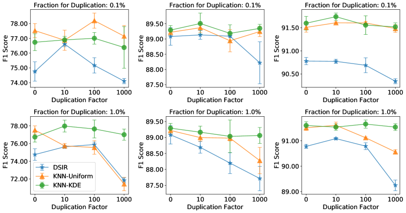
We evaluate the robustness of the selection methods against near-duplicates in the candidate examples. We follow the same evaluation protocol described in Section 5.2 while injecting duplicates to the candidate examples. We set different levels of duplication by varying the fraction of examples chosen for duplication and the duplication factor (number of duplicates per example). The fraction for duplication is set to 0.1% / 1%, and the duplication factor is set to 10 / 100 / 1000. For example, if the fraction for duplication is 0.1% and the duplication factor is 10, we randomly choose 0.1% of the examples from the data repository and duplicate each 10 times. We use ChemProt (1K), AGNews (3K), and IMDB (10K) to perform the analysis, where the numbers in the parentheses represent the sizes of the annotated data. We include KNN-Uniform with the same parameters as KNN-KDE to show the effectiveness of the KDE-based regularization.
The results show that KNN-KDE is the only method that is robust to all the duplication settings. We observe that under low duplication levels, specifically when (fraction for duplication, duplication factor) is (0.1%, 10), (0.1%, 100), or (1%, 10), all the methods perform similarly to the case without duplication. Given that the injected duplicates constitute less than 10% of the data repository in those settings, it is not surprising that they do not have much effect on the downstream performance. However, when the duplication factor is increased to 1000 with the fraction for duplication set to 0.1%, the performance of DSIR drops by 0.7 points on average, whereas KNN-KDE and KNN-Uniform retain their performance. Moreover, when the duplication factor is increased to 1000 with the fraction set to 1%, all the methods except KNN-KDE show a notable decline (more than 2 points on average) in their performance.
E.2 Runtime and Scalability
We report the runtime of our method that can be split into a pre-processing stage and a selection stage. We use a machine with an Intel(R) Xeon(R) Gold 5115 CPU @ 2.40GHz (40 cores) and 250GB RAM. The example embedding is computed using an NVIDIA Tesla V100 GPU with 32GB memory, while the other computations are on the CPU. In the pre-processing stage, our method embeds the candidate examples in the data repository and further builds indexes for the embeddings. This stage takes 28.38 hours for the data repository in Section 5.2 that contains 150M examples. In the selection stage, our method embeds the query examples, computes the probability assignment, and takes random samples according to the probability. This stage takes 0.7 hours for 10K query examples. The runtime of the selection stage scales linearly with the number of query examples and remains unaffected by the number of examples to be sampled except for the I/O cost. Note that while our method takes a substantial amount of time in the pre-processing stage, the cost is one-time and the index can be reused for a variety of tasks that require similarity search. In general, our methods are practical in terms of runtime.
E.3 Task-Specific Instruction Tuning for One epoch
In Section 5.1, we perform instruction tuning for 4 epochs, and our method takes a random sample in each epoch instead of using a fixed set. Therefore, the total number of unique examples can be up to 4x the number of examples used per epoch, though the actual number of unique examples is much lower since examples with high probability mass tend to be repeatedly sampled. To demonstrate that the number of unique examples during training is not the primary factor behind our performance gain, we provide additional results that compare our method with LESS when the number of epochs is set to . Specifically, each method selects a set whose size is 4% of the candidates. Then we train the model on the selected set for 1 epoch (the amount of computation is the same as using 1% for 4 epochs). The results are shown in Table 8. From the results, we can see that our method still outperforms LESS in 5 out of the 6 settings when LESS has access to more unique examples.
| Model | Llama-2-7b | Mistral-7B | ||||
| Dataset | TydiQA | MMLU | BBH | TydiQA | MMLU | BBH |
| LESS | ||||||
| Ours | ||||||
E.4 Domain-Specific Continued Pretraining with Different Selection Sizes
We compare with the baselines when the size of the selected data is 100K and 300K for domain-specific continued pretraining while the size of the annotated dataset is fixed to 3K. The other settings are the same as in Section 5.2. The results are in Table 9 which show that our method is either better than or comparable to the baselines.
| ——100K Sample Size —— | ——300K Sample Size —— | |||||||
| ChemP. | IMDB | SCI. | AGNews | ChemP. | IMDB | SCI. | AGNews | |
| Base | ||||||||
| Rand | ||||||||
| DSIR | ||||||||
| Ours | ||||||||
E.5 Micro-Benchmarks
In this section, we provide micro-benchmarks that study the effects of the hyperparameters in our framework. In addition, we show the performance of KNN-TV, an instantiation of our framework that is not covered in the main experiments. The experiments focus on domain-specific pretraining, following the same settings as in Section 5.2. The datasets and sizes used in the micro-benchmarks are ChemP (1K), AG (3K), and IMDB (10K).
E.5.1 Tradeoff between Distribution Alignment and Diversity
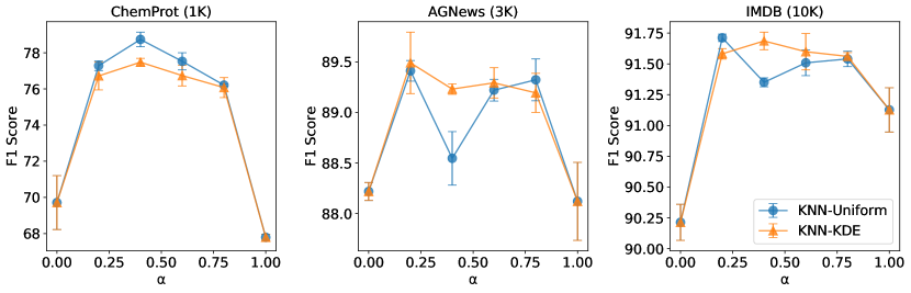
We study the effects of , the hyperparameter that controls the tradeoff between distribution alignment and diversity in our framework. We vary the value of in KNN-Uniform and KNN-KDE and report the F1 scores of the downstream tasks in Figure 3. In all three datasets, we observe a notable drop in F1 scores when or , and consistent performance when the value of is set to other values. Note that KNN-Uniform or KNN-KDE is equivalent to Uniform when , and transports all the probability mass of each query example to its -nearest-neighbor in the data repository when . The former does not consider distribution alignment, while the latter results in overfitting to the -nearest-neighbors. For the other values of , we report the corresponding neighborhood size (the final in KNN-Uniform and the average of the final in KNN-KDE) in Table 12. The consistent performance with shows that our framework is not sensitive to the choice of .
E.5.2 Effects of Kernel Size in KNN-KDE
We vary the kernel size for the kernel density estimation in KNN-KDE. The performance is shown in Table 10. The F1 scores of all three downstream tasks are consistent across different choices of kernel size. The results show that the performance of KNN-KDE is not sensitive to the choice of kernel size.
| Kernel Size | |||
| ChemProt (1K) | |||
| AGNews (3K) | |||
| IMDB (10K) |
E.5.3 Performance of KNN-TV
We evaluate KNN-TV () and show the results in Table 11. KNN-TV performs similarly to KNN-KDE , and significantly worse than KNN-KDE . The reason is that KNN-TV assigns almost all the probability mass (more than 99.99%) to the -nearest neighbor of each query example and causes overfitting to them, a behavior similar to KNN-KDE .
| Dataset | ChemProt (1K) | AGNews (3K) | IMDB (10K) |
| KNN-TV | |||
| KNN-KDE () | |||
| KNN-KDE () |
| Dataset | ChemProt (1K) | AGNews (3K) | IMDB (10K) |
| 959 / 993 | 813 / 830 | 918 / 928 | |
| 398 / 408 | 342 / 346 | 372 / 373 | |
| 189 / 191 | 165 / 164 | 177 / 174 | |
| 76 / 74 | 69 / 65 | 72 / 68 |
NeurIPS Paper Checklist
-
1.
Claims
-
Question: Do the main claims made in the abstract and introduction accurately reflect the paper’s contributions and scope?
-
Answer: [Yes]
-
Justification: We clearly state our contributions and scope in the abstract and introduction.
-
Guidelines:
-
•
The answer NA means that the abstract and introduction do not include the claims made in the paper.
-
•
The abstract and/or introduction should clearly state the claims made, including the contributions made in the paper and important assumptions and limitations. A No or NA answer to this question will not be perceived well by the reviewers.
-
•
The claims made should match theoretical and experimental results, and reflect how much the results can be expected to generalize to other settings.
-
•
It is fine to include aspirational goals as motivation as long as it is clear that these goals are not attained by the paper.
-
•
-
2.
Limitations
-
Question: Does the paper discuss the limitations of the work performed by the authors?
-
Answer: [Yes]
-
Justification: We discuss the limitations in the conclusion.
-
Guidelines:
-
•
The answer NA means that the paper has no limitation while the answer No means that the paper has limitations, but those are not discussed in the paper.
-
•
The authors are encouraged to create a separate "Limitations" section in their paper.
-
•
The paper should point out any strong assumptions and how robust the results are to violations of these assumptions (e.g., independence assumptions, noiseless settings, model well-specification, asymptotic approximations only holding locally). The authors should reflect on how these assumptions might be violated in practice and what the implications would be.
-
•
The authors should reflect on the scope of the claims made, e.g., if the approach was only tested on a few datasets or with a few runs. In general, empirical results often depend on implicit assumptions, which should be articulated.
-
•
The authors should reflect on the factors that influence the performance of the approach. For example, a facial recognition algorithm may perform poorly when image resolution is low or images are taken in low lighting. Or a speech-to-text system might not be used reliably to provide closed captions for online lectures because it fails to handle technical jargon.
-
•
The authors should discuss the computational efficiency of the proposed algorithms and how they scale with dataset size.
-
•
If applicable, the authors should discuss possible limitations of their approach to address problems of privacy and fairness.
-
•
While the authors might fear that complete honesty about limitations might be used by reviewers as grounds for rejection, a worse outcome might be that reviewers discover limitations that aren’t acknowledged in the paper. The authors should use their best judgment and recognize that individual actions in favor of transparency play an important role in developing norms that preserve the integrity of the community. Reviewers will be specifically instructed to not penalize honesty concerning limitations.
-
•
-
3.
Theory Assumptions and Proofs
-
Question: For each theoretical result, does the paper provide the full set of assumptions and a complete (and correct) proof?
-
Answer: [Yes]
-
Justification: Each theorem comes with a clear statement of the assumptions and proofs are provided in the appendix.
-
Guidelines:
-
•
The answer NA means that the paper does not include theoretical results.
-
•
All the theorems, formulas, and proofs in the paper should be numbered and cross-referenced.
-
•
All assumptions should be clearly stated or referenced in the statement of any theorems.
-
•
The proofs can either appear in the main paper or the supplemental material, but if they appear in the supplemental material, the authors are encouraged to provide a short proof sketch to provide intuition.
-
•
Inversely, any informal proof provided in the core of the paper should be complemented by formal proofs provided in appendix or supplemental material.
-
•
Theorems and Lemmas that the proof relies upon should be properly referenced.
-
•
-
4.
Experimental Result Reproducibility
-
Question: Does the paper fully disclose all the information needed to reproduce the main experimental results of the paper to the extent that it affects the main claims and/or conclusions of the paper (regardless of whether the code and data are provided or not)?
-
Answer: [Yes]
-
Justification: The details and hyperparameters of the experiments are provided in the appendix.
-
Guidelines:
-
•
The answer NA means that the paper does not include experiments.
-
•
If the paper includes experiments, a No answer to this question will not be perceived well by the reviewers: Making the paper reproducible is important, regardless of whether the code and data are provided or not.
-
•
If the contribution is a dataset and/or model, the authors should describe the steps taken to make their results reproducible or verifiable.
-
•
Depending on the contribution, reproducibility can be accomplished in various ways. For example, if the contribution is a novel architecture, describing the architecture fully might suffice, or if the contribution is a specific model and empirical evaluation, it may be necessary to either make it possible for others to replicate the model with the same dataset, or provide access to the model. In general. releasing code and data is often one good way to accomplish this, but reproducibility can also be provided via detailed instructions for how to replicate the results, access to a hosted model (e.g., in the case of a large language model), releasing of a model checkpoint, or other means that are appropriate to the research performed.
-
•
While NeurIPS does not require releasing code, the conference does require all submissions to provide some reasonable avenue for reproducibility, which may depend on the nature of the contribution. For example
-
(a)
If the contribution is primarily a new algorithm, the paper should make it clear how to reproduce that algorithm.
-
(b)
If the contribution is primarily a new model architecture, the paper should describe the architecture clearly and fully.
-
(c)
If the contribution is a new model (e.g., a large language model), then there should either be a way to access this model for reproducing the results or a way to reproduce the model (e.g., with an open-source dataset or instructions for how to construct the dataset).
-
(d)
We recognize that reproducibility may be tricky in some cases, in which case authors are welcome to describe the particular way they provide for reproducibility. In the case of closed-source models, it may be that access to the model is limited in some way (e.g., to registered users), but it should be possible for other researchers to have some path to reproducing or verifying the results.
-
(a)
-
•
-
5.
Open access to data and code
-
Question: Does the paper provide open access to the data and code, with sufficient instructions to faithfully reproduce the main experimental results, as described in supplemental material?
-
Answer: [Yes]
-
Justification: All the data used are open-sourced. We have included the code in the Supplementary material.
-
Guidelines:
-
•
The answer NA means that paper does not include experiments requiring code.
-
•
Please see the NeurIPS code and data submission guidelines (https://nips.cc/public/guides/CodeSubmissionPolicy) for more details.
-
•
While we encourage the release of code and data, we understand that this might not be possible, so “No” is an acceptable answer. Papers cannot be rejected simply for not including code, unless this is central to the contribution (e.g., for a new open-source benchmark).
-
•
The instructions should contain the exact command and environment needed to run to reproduce the results. See the NeurIPS code and data submission guidelines (https://nips.cc/public/guides/CodeSubmissionPolicy) for more details.
-
•
The authors should provide instructions on data access and preparation, including how to access the raw data, preprocessed data, intermediate data, and generated data, etc.
-
•
The authors should provide scripts to reproduce all experimental results for the new proposed method and baselines. If only a subset of experiments are reproducible, they should state which ones are omitted from the script and why.
-
•
At submission time, to preserve anonymity, the authors should release anonymized versions (if applicable).
-
•
Providing as much information as possible in supplemental material (appended to the paper) is recommended, but including URLs to data and code is permitted.
-
•
-
6.
Experimental Setting/Details
-
Question: Does the paper specify all the training and test details (e.g., data splits, hyperparameters, how they were chosen, type of optimizer, etc.) necessary to understand the results?
-
Answer: [Yes]
-
Justification: The training and test details are in the appendix.
-
Guidelines:
-
•
The answer NA means that the paper does not include experiments.
-
•
The experimental setting should be presented in the core of the paper to a level of detail that is necessary to appreciate the results and make sense of them.
-
•
The full details can be provided either with the code, in appendix, or as supplemental material.
-
•
-
7.
Experiment Statistical Significance
-
Question: Does the paper report error bars suitably and correctly defined or other appropriate information about the statistical significance of the experiments?
-
Answer: [Yes]
-
Justification: Error bars are reported for every experimental result.
-
Guidelines:
-
•
The answer NA means that the paper does not include experiments.
-
•
The authors should answer "Yes" if the results are accompanied by error bars, confidence intervals, or statistical significance tests, at least for the experiments that support the main claims of the paper.
-
•
The factors of variability that the error bars are capturing should be clearly stated (for example, train/test split, initialization, random drawing of some parameter, or overall run with given experimental conditions).
-
•
The method for calculating the error bars should be explained (closed form formula, call to a library function, bootstrap, etc.)
-
•
The assumptions made should be given (e.g., Normally distributed errors).
-
•
It should be clear whether the error bar is the standard deviation or the standard error of the mean.
-
•
It is OK to report 1-sigma error bars, but one should state it. The authors should preferably report a 2-sigma error bar than state that they have a 96% CI, if the hypothesis of Normality of errors is not verified.
-
•
For asymmetric distributions, the authors should be careful not to show in tables or figures symmetric error bars that would yield results that are out of range (e.g. negative error rates).
-
•
If error bars are reported in tables or plots, The authors should explain in the text how they were calculated and reference the corresponding figures or tables in the text.
-
•
-
8.
Experiments Compute Resources
-
Question: For each experiment, does the paper provide sufficient information on the computer resources (type of compute workers, memory, time of execution) needed to reproduce the experiments?
-
Answer: [Yes]
-
Justification: The hardware we use is reported in the appendix.
-
Guidelines:
-
•
The answer NA means that the paper does not include experiments.
-
•
The paper should indicate the type of compute workers CPU or GPU, internal cluster, or cloud provider, including relevant memory and storage.
-
•
The paper should provide the amount of compute required for each of the individual experimental runs as well as estimate the total compute.
-
•
The paper should disclose whether the full research project required more compute than the experiments reported in the paper (e.g., preliminary or failed experiments that didn’t make it into the paper).
-
•
-
9.
Code Of Ethics
-
Question: Does the research conducted in the paper conform, in every respect, with the NeurIPS Code of Ethics https://neurips.cc/public/EthicsGuidelines?
-
Answer: Yes
-
Justification: We have reviewed the NeurIPS Code of Ethics and confirm that our research conforms it.
-
Guidelines:
-
•
The answer NA means that the authors have not reviewed the NeurIPS Code of Ethics.
-
•
If the authors answer No, they should explain the special circumstances that require a deviation from the Code of Ethics.
-
•
The authors should make sure to preserve anonymity (e.g., if there is a special consideration due to laws or regulations in their jurisdiction).
-
•
-
10.
Broader Impacts
-
Question: Does the paper discuss both potential positive societal impacts and negative societal impacts of the work performed?
-
Answer: [Yes]
-
Justification: We have such discussion in the introduction and the conclusion.
-
Guidelines:
-
•
The answer NA means that there is no societal impact of the work performed.
-
•
If the authors answer NA or No, they should explain why their work has no societal impact or why the paper does not address societal impact.
-
•
Examples of negative societal impacts include potential malicious or unintended uses (e.g., disinformation, generating fake profiles, surveillance), fairness considerations (e.g., deployment of technologies that could make decisions that unfairly impact specific groups), privacy considerations, and security considerations.
-
•
The conference expects that many papers will be foundational research and not tied to particular applications, let alone deployments. However, if there is a direct path to any negative applications, the authors should point it out. For example, it is legitimate to point out that an improvement in the quality of generative models could be used to generate deepfakes for disinformation. On the other hand, it is not needed to point out that a generic algorithm for optimizing neural networks could enable people to train models that generate Deepfakes faster.
-
•
The authors should consider possible harms that could arise when the technology is being used as intended and functioning correctly, harms that could arise when the technology is being used as intended but gives incorrect results, and harms following from (intentional or unintentional) misuse of the technology.
-
•
If there are negative societal impacts, the authors could also discuss possible mitigation strategies (e.g., gated release of models, providing defenses in addition to attacks, mechanisms for monitoring misuse, mechanisms to monitor how a system learns from feedback over time, improving the efficiency and accessibility of ML).
-
•
-
11.
Safeguards
-
Question: Does the paper describe safeguards that have been put in place for responsible release of data or models that have a high risk for misuse (e.g., pretrained language models, image generators, or scraped datasets)?
-
Answer: [N/A]
-
Justification: This paper does not introduce new models or datasets.
-
Guidelines:
-
•
The answer NA means that the paper poses no such risks.
-
•
Released models that have a high risk for misuse or dual-use should be released with necessary safeguards to allow for controlled use of the model, for example by requiring that users adhere to usage guidelines or restrictions to access the model or implementing safety filters.
-
•
Datasets that have been scraped from the Internet could pose safety risks. The authors should describe how they avoided releasing unsafe images.
-
•
We recognize that providing effective safeguards is challenging, and many papers do not require this, but we encourage authors to take this into account and make a best faith effort.
-
•
-
12.
Licenses for existing assets
-
Question: Are the creators or original owners of assets (e.g., code, data, models), used in the paper, properly credited and are the license and terms of use explicitly mentioned and properly respected?
-
Answer: [Yes]
-
Justification: We use open-source models and data, which have been properly cited.
-
Guidelines:
-
•
The answer NA means that the paper does not use existing assets.
-
•
The authors should cite the original paper that produced the code package or dataset.
-
•
The authors should state which version of the asset is used and, if possible, include a URL.
-
•
The name of the license (e.g., CC-BY 4.0) should be included for each asset.
-
•
For scraped data from a particular source (e.g., website), the copyright and terms of service of that source should be provided.
-
•
If assets are released, the license, copyright information, and terms of use in the package should be provided. For popular datasets, paperswithcode.com/datasets has curated licenses for some datasets. Their licensing guide can help determine the license of a dataset.
-
•
For existing datasets that are re-packaged, both the original license and the license of the derived asset (if it has changed) should be provided.
-
•
If this information is not available online, the authors are encouraged to reach out to the asset’s creators.
-
•
-
13.
New Assets
-
Question: Are new assets introduced in the paper well documented and is the documentation provided alongside the assets?
-
Answer: [Yes]
-
Justification: The code is well documented.
-
Guidelines:
-
•
The answer NA means that the paper does not release new assets.
-
•
Researchers should communicate the details of the dataset/code/model as part of their submissions via structured templates. This includes details about training, license, limitations, etc.
-
•
The paper should discuss whether and how consent was obtained from people whose asset is used.
-
•
At submission time, remember to anonymize your assets (if applicable). You can either create an anonymized URL or include an anonymized zip file.
-
•
-
14.
Crowdsourcing and Research with Human Subjects
-
Question: For crowdsourcing experiments and research with human subjects, does the paper include the full text of instructions given to participants and screenshots, if applicable, as well as details about compensation (if any)?
-
Answer: [N/A]
-
Justification: We do not have such experiments.
-
Guidelines:
-
•
The answer NA means that the paper does not involve crowdsourcing nor research with human subjects.
-
•
Including this information in the supplemental material is fine, but if the main contribution of the paper involves human subjects, then as much detail as possible should be included in the main paper.
-
•
According to the NeurIPS Code of Ethics, workers involved in data collection, curation, or other labor should be paid at least the minimum wage in the country of the data collector.
-
•
-
15.
Institutional Review Board (IRB) Approvals or Equivalent for Research with Human Subjects
-
Question: Does the paper describe potential risks incurred by study participants, whether such risks were disclosed to the subjects, and whether Institutional Review Board (IRB) approvals (or an equivalent approval/review based on the requirements of your country or institution) were obtained?
-
Answer: [N/A]
-
Justification: We do not have this type of studies.
-
Guidelines:
-
•
The answer NA means that the paper does not involve crowdsourcing nor research with human subjects.
-
•
Depending on the country in which research is conducted, IRB approval (or equivalent) may be required for any human subjects research. If you obtained IRB approval, you should clearly state this in the paper.
-
•
We recognize that the procedures for this may vary significantly between institutions and locations, and we expect authors to adhere to the NeurIPS Code of Ethics and the guidelines for their institution.
-
•
For initial submissions, do not include any information that would break anonymity (if applicable), such as the institution conducting the review.
-
•