GCLS²: Towards Efficient Community Detection using Graph Contrastive Learning with Structure Semantics

Abstract

Due to powerful ability to learn representations from unlabeled graphs, graph contrastive learning (GCL) has shown excellent performance in community detection tasks. Existing GCL-based methods on the community detection usually focused on learning attribute representations of individual nodes, which, however, ignores structure semantics of communities (e.g., nodes in the same community should be close to each other). Therefore, in this paper, we will consider the semantics of community structures for the community detection, and propose an effective framework of graph contrastive learning under structure semantics (GCLS²) for detecting communities. To seamlessly integrate interior dense and exterior sparse characteristics of communities with our contrastive learning strategy, we employ classic community structures to extract high-level structural views and design a structure semantic expression module to augment the original structural feature representation. Moreover, we formulate the structure contrastive loss to optimize the feature representation of nodes, which can better capture the topology of communities. Extensive experiments have been conducted on various real-world graph datasets and confirmed that GCLS² outperforms eight state-of-the-art methods, in terms of the accuracy and modularity of the detected communities.

I Introduction

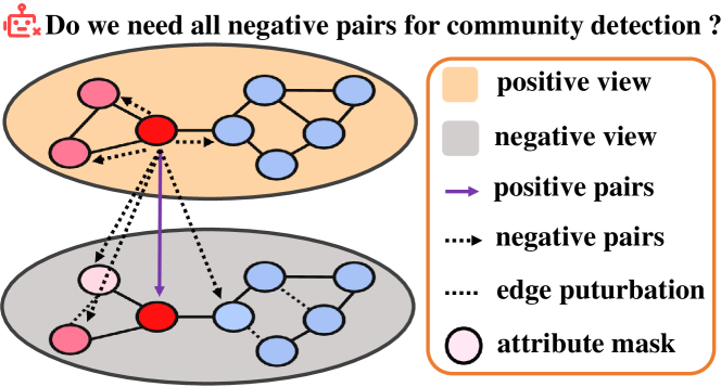
(a) GCL-based community detection

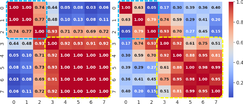
(b) similarity matrix heatmap

Figure 1: A motivation example of graph structure semantics contrastive learning on the community detection.

The community detection (CD) is one of fundamental and important problems in graph data analysis, and it plays an important role in many real-world applications such as the protein function prediction [1], social network analysis [2, 3], anomaly detection [4], and many others. Although traditional CD methods (e.g., hierarchical clustering [5], spectral clustering [6], optimization-based methods [7], etc.) can achieve high accuracy, they often incur high time costs and/or have poor scalability issue for conducting CD over large-scale data graphs, which limits these methods from being widely used in practical applications.

On the other hand, the supervised learning methods [8, 9] have been used for CD tasks by mining from graph data, which take data graphs as the input through an end-to-end graph deep learning model, and output community prediction results via the trained neural networks. However, such supervised learning methods rely heavily on manually labeled data and have poor generalization performance due to the overfitting.

Recently, with the success of unsupervised contrastive learning in image and text representation learning, the graph contrastive learning (GCL) paradigms (e.g., InfoNCE [10], GRACE [11], GCA [12], etc.) have been widely adopted on graphs in various graph-related tasks (e.g., link prediction and node classification), due to their excellent learning capability of the node information. However, these GCL-based methods do not consider structural relationships among nodes in communities, which incurs a reduction in the accuracy and modularity of the detected communities.

Motivation: Figure 1(a) shows a traditional GCL-based (GRACE [11]) community detection framework with two communities (i.e., red and blue groups), which first obtains negative views via data augmentation methods (e.g., edge perturbation, attribute mask, etc.), then constructs positive pairs (e.g., different views of the same nodes) and negative pairs (e.g., different views of neighbor nodes), and finally trains a model to minimize vector distances between positive pairs, while maximizing vector distances between negative pairs. However, intuitively, the feature vector distances of nodes in the red community (same as the blue community) should be close to each other, while the traditional GCL pulls them farther apart. Figure 1(b) shows the heatmaps of the node similarity matrix from a 2-layer DNN applied to the data graph in Figure 1(a), comparing to the results with (left) and without (right) traditional GCL. From Figure 1(b), we observe that nodes expected to belong to the same community (e.g., those within blue and gold boxes) become less similar after GCL training, which will lead to low accuracy and modularity in community detection. This is because the nodes in the same community should be close to each other, while those from different communities should be distant, rather than all nodes in the data graph being pulled apart.

To tackle the aforementioned community detection problem, in this paper, we propose a graph contrastive learning framework under structure semantics for the community detection, named GCLS². Specifically, we start from the community structure, and apply structure semantic contrastive learning to obtain better feature representation of nodes by extracting structure semantics of graph data. We construct a graph preprocessing module, using existing community dense structures (e.g., $k$-core [13], $k$-truss [14], and $k$-clique [15]) to obtain high-level and original structure views. For different views, we use a structure similarity semantic expression model to obtain structure features of the data graph and design structure contrastive learning to fine-tune node structure feature representations of graph data specific to the community detection task.

Contributions: The main contributions of this paper are summarized as follows:

• We analyze the limitations of traditional GCL methods for the community detection task and explore a structure-driven approach to obtain better representation features.

• We propose a Graph Contrastive Learning with Structure Semantics (GCLS²) framework that can effectively extract structural representations of data graphs for community detection.

• We design a Structure Similarity Semantic (SSS) expression module in our proposed GCLS² framework to enhance the feature representation of structures.

• Through extensive experiments, we confirm that our proposed GCLS² outperforms the supervised and unsupervised learning baselines for community detection.

II Related Work

Community Detection: The community detection can be classified into traditional and deep learning methods. The former one mainly explores communities from network structure with clustering and optimization algorithms [16, 17], whereas the latter one utilizes deep learning to uncover deep network information and model complex relationships from high-dimensional attribute data to lower-dimensional vectors. Due to complex topology structures and attribute features for real-world networks, high computational costs make traditional methods less applicable to practical applications. However, existing deep learning methods (e.g., GCN [18] and GAT [19]) rely on real labels and attributes of the data graph and pay little attention to the important structure of communities. In contrast, our GCLS² method starts from unsupervised learning that does not rely on real labels and attributes. Moreover, GCLS² performs effective community detection by mining the structure information of the community.

Graph Contrastive Learning: The graph contrastive learning optimizes the representation of nodes, by maximizing the agreement between pairs of positive samples and minimizing the agreement between pairs of negative samples to be adapted to various downstream tasks. For the node level, there are two general contrastive ways: i) node-graph, for example, DGI [20] contrasts node feature embeddings of augmented view and original data graph with graph feature embeddings of the original data graph, and MVGRL [21] contrasts node feature embeddings of one view with the graph feature embeddings of another view, ii) node-node, for example, GRACE [11] contrasts node feature embeddings of two augmented views with each other, and NCLA [22] contrasts neighbors’ feature embeddings of multiple augmented views. Although these contrastive learning methods have made greater progress in the feature representation, most contrasted samples in the community detection task are against the community’s inherent information representation, where feature embedding representations within communities should be similar and feature embedding representations between communities should be dissimilar. Our proposed GCLS² approach uses high-level structure adjacency matrix as a signal to guide the anchor closer to dense intra-community and away from the inter-community, and achieves good detection results even when using community structure information only.

III Preliminaries

In this section, we give the definitions of the graph data model and the community detection problem.

III-A Graph Data Model

We first provide the formal definition of a data graph $G$.

Definition 1.

(Data Graph, $G$) A data graph $G$ is in the form of a quintuple $(V(G),E(G),\Phi(G),A,X)$, where $V(G)$ is a set of nodes, $v_{i}$, $E(G)$ represents a set of edges $e(v_{i},v_{j})$ (connecting two ending nodes $v_{i}$ and $v_{j}$), $\Phi(G)$ is a mapping function: $V(G)\times V(G)\rightarrow E(G)$, and $A\in\mathbb{R}^{N\times N}$ and $X\in\mathbb{R}^{N\times F}$ are the adjacency and attribute matrices, respectively. Here, $A_{ij}=1$, if $(v_{i},v_{j})\in E(G)$, and $X$ contains attribute vectors, $x_{i}\in\mathbb{R}^{F}$, of $N$ vertices $v_{i}$.

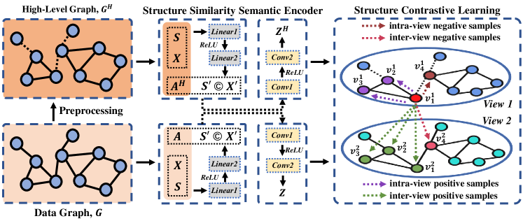
Figure 2: Overview of our GCLS² framework. The \scriptsize{C}⃝ denotes the concatenation of vectors.

Definition 1 defines the data graph model, which is useful in many real applications such as social networks [14, 23], transportation networks [24], and bioinformatic networks [25, 26].

III-B Community Detection

The community detection is a fundamental task in the network analysis. The target is to partition the data graph into multiple subgraphs (i.e., communities) that are internally dense and externally sparse. The resulting communities can be used to uncover important structures and patterns within complex networks and extract valuable knowledge from network data in diverse domains.

Formally, we define the community detection as follows.

Definition 2.

(Community Detection, CD) Given a data Graph $G$ and a positive integer parameter $L$, the community detection (CD) problem obtains a set of disjoint subgraphs (i.e., communities), $g=\{g_{1},g_{2},\cdots,g_{L}\}$, in the data graph $G$, where each community $g_{i}$ ($1\leq i\leq L$) in $g$ contains classic community structures (e.g., $k$-core, $k$-truss, $k$-plex, etc.).

In the literature of social networks, the commonly-used dense community semantics with high structural cohesiveness include $k$-core [27], $k$-truss [14], and $k$-plex [28]. Specifically, for $k$-core, the degree of each node in $g$ is greater than or equal to $k$; for $k$-truss, each edge is contained in at least $(k-2)$ triangles; for $k$-plex, the degree of each node in $g$ is greater than $(|V(g)|-k)$.

IV Methodology

In this section, we present our proposed GCLS² approach in detail. First, we will briefly discuss our framework. Then, we will detail the graph augmentation method for high-level structure and an encoder for extracting graph structure similarity semantics. After that, we will introduce how to design the structure contrastive loss.

IV-A Framework

Figure 2 shows the overall framework of GCLS². First, we use the classical community structure to extract the high-level structure graph $G^{H}$ from the data graph $G$ for preprocessing, then we obtain the structure similarity semantic vectors of the data graph and the high-level structure graph through structural similarity matrix computation and semantic encoding, and we obtain the feature representations of the two graphs by GCN encoder. After that, we use the feature representations for the structure contrastive learning so that the features better match the structure semantic information of community detection.

IV-B Graph Preprocessing

In GCLS² model, the graph preprocessing is used to obtain the high-level graph that deeply expresses the structure information of the graph. We show an example of the graph preprocessing in Figure 3. For a data graph $G=(V(G),E(G),\Phi(G),A,X)$, we have the adjacency matrix $A\in\{0,1\}^{N\times N}$ and arrtibute matrix $X\in\mathbb{R}^{N\times F}$, where $N$ denotes the size of $V(G)$ and $F$ denotes the number of attributes. We consider using a set, $M=\{M_{1},M_{2},\cdots,M_{m}\}$, of the classical community structure patterns (i.e., $k$-core, $k$-truss, $k$-plex, etc.) to extract the high-level structure of $G$. Specifically, we count the substructures of the original graph using each pattern $M_{i}\in M$, and we initialize a dictionary $Dic$ to store the number of specific substructural patterns held for each edge pair $\left\langle v_{i},v_{j}\right\rangle$. In Figure 3, we use two substructures (triangle and pentagon, which are 1-core and 3-plex structures, respectively) for pattern counting, and the dashed lines in Figure 3 denote the edges with a pattern count of 0 and masked. In this way, we can obtain a high-level structure graph $G^{H}$ and a high-level adjacency matrix $A^{H}$. It is worth noting that we did not remove those nodes whose neighboring edges all have a pattern number of 0, and retained their attribute values for subsequent structure contrastive learning to maintain model smoothing.

After that, we extract the elements of the dictionary $Dic$ and construct a structure similarity matrix $S\in\mathbb{R}^{N\times N}$ for $G$ and $G^{H}$, the computation of each $s_{i,j}\in S$ as follows:

$$s_{i,j}=\frac{Dic(v_{i},v_{j})+1}{max(Dic(\cdot))+1}$$ (1)

where $max(Dic(\cdot))$ denotes the maximum value of the pattern count in the dictionary $Dic$. The $S$ represents high-level structure features in $G$ and $G^{H}$ that can deeply represent structure aggregation information.

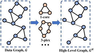
Figure 3: An example of graph preprocessing.

IV-C Structure Similarity Semantic Encoder

Different from most of the previous graph encoders that directly convolve the attribute matrix $X$ and the adjacency matrix $A$ to extract graph features, we design a structure similarity semantic (SSS) module to extract the semantic representations of structures and attributes for low-level features $S^{\prime}$ and $X^{\prime}$, which is to be able to better provide a more intuitive semantic representation for subsequent graph feature extraction. For the structure similarity matrix $S$ and attribute matrix $X$, we use a two-layer DNN $f:\mathbb{R}^{N\times N}\rightarrow\mathbb{R}^{N\times d}$ for semantic features $S^{\prime}$ and $X^{\prime}$, that is:

$$S^{\prime}=f(S)=W^{(2)}_{dnn}(\sigma(W^{(1)}_{dnn}S+b^{(1)}_{dnn}))+b^{(2)}_{dnn}$$ (2)

$$X^{\prime}=f(X)=W^{(2)}_{dnn}(\sigma(W^{(1)}_{dnn}X+b^{(1)}_{dnn}))+b^{(2)}_{dnn}$$ (3)

where $\sigma(\cdot)$ denotes the ReLU activation function, $W_{dnn}$ is the neural network trainable weight parameters, and $b_{dnn}$ is the bias. The (1) and (2) denote the 1-th layer and 2-th layer, respectively. The second term of the equation represents the process of message-passing in the DNN network. The output dimensions of both features are $d$.

Then, to encode the attribute semantic feature $X^{\prime}$ and the structure similarity semantic feature $S^{\prime}$ into a unified graph feature space without destroying the respective semantic representations, we aggregate the two features by concatenation and use them in the subsequent feature extraction.

Next, we learn a GCN encoder $\mathbb{F}:\mathbb{R}^{N\times N}\times\mathbb{R}^{N\times 2d}\rightarrow\mathbb{R}^{N\times L}$ to obtain the node representations of $G$ and $G^{H}$, where $L$ denotes the output dimension of the encoder, both of which share weights during the learning process. The input of $G$ is $(A,AGG(S^{\prime},X^{\prime}))$ and the input of $G^{H}$ is $(A^{H},AGG(S^{\prime},X^{\prime}))$, where the $AGG(\cdot)$ is concatenation aggregated function. So that we can obtain the node features $Z\in\mathbb{R}^{N\times L}$ of the graph by the generalized equation:

$$Z=\mathbb{F}(A,AGG(S^{\prime},X^{\prime}))=\{z_{i}|v_{i}\in V(G)\}$$ (4)

The detailed message-passing process of GCN is as follows:

$$z_{i}^{(l+1)}=\sigma(\sum_{v_{j}\in N(v_{i})}\hat{D}^{-\frac{1}{2}}\hat{A}\hat{D}^{-\frac{1}{2}}z_{j}^{(l)}W^{(l)}_{gcn}+b^{(l)}_{gcn})$$ (5)

where $l$ denotes the l-th layer, $\hat{A}=A+I$ denotes the message self-passage, $I$ denotes the unit matrix, $D$ denotes the degree matrix, $\sigma(\cdot)$ denotes the activation function, we use the ReLU in GCLS², the $W_{gcn}$ and $b_{gcn}$ denote the trainable weight parameters and bias in GCN and the $N(v_{i})$ denotes the neighbors of $v_{i}$. The 0-th node features as follows:

$$z_{i}^{(0)}=AGG(s_{i}^{{}^{\prime}},x_{i}^{{}^{\prime}})|s_{i}^{{}^{\prime}}\in S^{\prime},x_{i}^{{}^{\prime}}\in X^{\prime}$$ (6)

Similarly, for the high-level structure graph $G^{H}$, the representation of node features is as follows:

$$Z^{H}=\mathbb{F}(A^{H},AGG(S^{\prime},X^{\prime}))=\{z_{i}|v_{i}\in V(G^{H})\}$$ (7)

The detailed message-passing is the same as the graph $G$.

IV-D Structure Contrastive Learning

Most existing GCL methods overlooked that nodes within a community should have similar representations, while inter-community nodes should differ. Therefore, we proposed a structure contrastive learning, which uses the graph’s high-level structure to divide the positive and negative pairs of the GCL for structure learning, thereby enhancing the community representation of nodes.

Since GCLS² does not use an activation function in the last layer of the GCN, we will do $L_{2}$-normalization on the learned node representations to ensure that the magnitude of the data is uniform before the structure contrastive learning. Moreover, we take the original data graph $G$ and high-level structure graph $G^{H}$ as two views for structure contrastive learning, which is because the $G$ is unmodified and contains accurate and rich graph-based information, and the $G^{H}$ contains rich and dense community information.

Let $z_{i}^{1}$ and $z_{i}^{2}$ denote the $v_{i}$’s $L_{2}$-normalized embedding learned by view 1 and view 2, respectively. We consider $z_{i}^{1}$ as an anchor, where there are two positive sample pairs: i) intra-view high-level neighbors in the same dense structure, i.e., $\{z_{j}^{1}|v_{j}\in N(v_{i})^{H}\}$; ii) inter-view high-level neighbors in the same dense structure, i.e., $\{z_{i}^{2},z_{j}^{2}|v_{j}\in N(v_{i})^{H}\}$. Then, the number of positive sample pairs with anchor $z_{i}^{1}$ is $2|N(v_{i})^{H}|+1$, where $|N(v_{i})^{H}|$ denotes the number of neighbors of $v_{i}$ in high-level structure graph $G^{H}$. With the rest formed two negative sample pairs: i) intra-view nodes not in the high-level neighbors, i.e., $\{z_{j}^{1}|v_{j}\notin N(v_{i})^{H}\}$; ii) inter-view not in the high-level neighbors, i.e., $\{z_{i}^{2},z_{j}^{2}|v_{j}\notin N(v_{i})^{H}\}$. Finally, the structure contrastive loss of $z_{i}^{1}$ between view 1 and view 2 is formulated as:

$$pos(z_{i}^{1})=\sum\limits_{v_{j}\in N(v_{i})^{H}}(e^{sim(z_{i}^{1},z_{j}^{1})/\tau}+e^{sim(z_{i}^{1},z_{j}^{2})/\tau})$$ (8)

$$neg(z_{i}^{1}) =\sum\limits_{v_{j}\notin N(v_{i})^{H}}(e^{sim(z_{i}^{1},z_{j}^{1})/\tau}+e^{sim(z_{i}^{1},z_{j}^{2})/\tau})$$ (9)

$$\ell(z_{i}^{1})=-log\frac{(pos(z_{i}^{1})+e^{sim(z_{i}^{1},z_{i}^{2})/\tau})/(2|N(v_{i})^{H}|+1)}{neg(z_{i}^{1})+pos(z_{i}^{1})+e^{sim(z_{i}^{1},z_{i}^{2})/\tau}}$$ (10)

where the $sim(z_{i},z_{j})=z_{i}\cdot z_{j}$ denotes the vector similarity between $z_{i}$ and $z_{j}$, and $\tau$ denotes a temperature parameter.

Since the structure contrastive learning is computed at the embedding level of the nodes, to simplify the representation, we use $v_{i}$ instead of $z_{i}$ in the Structure Contrastive Learning of Figure 2 as an example. We set $v_{1}^{1}$ as the anchor, then the positive sample pairs of $v_{1}^{1}$ have: i) the intra-view, {$\left\langle v_{1}^{1},v_{2}^{1}\right\rangle$, $\left\langle v_{1}^{1},v_{3}^{1}\right\rangle$}; ii) the inter-view, {$\left\langle v_{1}^{1},v_{1}^{2}\right\rangle$, $\left\langle v_{1}^{1},v_{2}^{2}\right\rangle$, $\left\langle v_{1}^{1},v_{3}^{2}\right\rangle$}. The negative sample pairs of $v_{1}^{1}$ have: i) the intra-view, {$\left\langle v_{1}^{1},v_{4}^{1}\right\rangle$, $\cdots$, $\left\langle v_{1}^{1},v_{n}^{1}\right\rangle$}; ii) the inter-view, {$\left\langle v_{1}^{1},v_{4}^{2}\right\rangle$, $\cdots$, $\left\langle v_{1}^{1},v_{n}^{2}\right\rangle$}.

Minimizing Eq. 10 will maximize the agreement between pairs of positive samples and minimize the agreement of pairs of negative samples. Through the computational propagation of mutual information between nodes, the feature representations of each node will agree with the high-level structure pattern’s feature representations within the other view itself and between the intra-view and inter-view.

Since the two views are symmetric, the node structure contrastive loss of the other view $\ell(z_{i}^{2})$ is defined similarly to Eq. 10. Then we minimize the loss mean of the two views to give the overall comparison loss as follows:

$$\mathcal{L}=\frac{1}{2N}\sum_{i=1}^{N}[\ell(z_{i}^{1})+\ell(z_{i}^{2})]$$ (11)

1   Input: i) the data graph $G$ with adjacency matrix $A$ and attribute matrix $X$, and ii) the number of training epochs $\varepsilon$

  Output: Features $Z$

1:  $G^{H}\leftarrow G$, $A^{H}\leftarrow A$

22:  $S\leftarrow$ Eq. 1 with ($G^{H}$)

3:  for epoch $\leftarrow 1,2,\cdots,\varepsilon$ do

4:     $S^{\prime}\leftarrow$ Eq. 2 with ($S$)

5:     $X^{\prime}\leftarrow$ Eq. 3 with ($X$)

6:     $Z\leftarrow$ Eq. 4 with ($A,AGG(S^{\prime},X^{\prime})$)

7:     $Z^{H}\leftarrow$ Eq. 7 with ($A^{H},AGG(S^{\prime},X^{\prime})$)

8:     $\mathcal{L}\leftarrow$ Eq. 11 with ($Z,Z^{H}$)

9:     repeat steps 4-8 to update the network parameters by gradient descent to minimize $\mathcal{L}$

10:  end for

11:  return  $Z$

Algorithm 1 GCLS² Training Algorithm

The detailed GCLS² training process is shown in Algorithm 1. Specifically, we first obtain the high-level structure graph $G^{H}$ and high-level adjacency matrix $A^{H}$ from the original data graph $G$, and then extract the structure similarity matrix $S$ from $G^{H}$ (lines 1-2). For each training iteration, we first use the SSS module to extract structural semantics $S^{\prime}$ and attribute semantics $X^{\prime}$ (lines 3-5). Next, we employ a GCN with weight shared to extract node features from both $G$ and $G^{H}$, resulting in the node feature matrix $Z$ and the high-level node feature matrix $Z^{H}$ (lines 6-7). After that, we adjust the network parameters by minimizing structure contrastive learning $\mathcal{L}$ on $Z$ and $Z^{H}$ (lines 8-9). Finally, after $\varepsilon$ training iterations, we return the node features $Z$ obtained for subsequent community detection (lines 10-11).

TABLE I: Statistics of the tested real-world graph datasets. The “#Attrs.” denotes the number of attributes, the “NA” denotes no attributes, and the “#Comms.” denotes the number of communities.

Datasets	#Nodes	#Edges	Avg. Deg.	#Attrs.	#Comms.
Cora	2,708	5,429	4.01	1,433	7
Citeseer	3,327	4,732	2.84	3,703	6
PubMed	19,717	44,338	4.50	500	3
CoauthorCS	18,333	81,894	8.93	6,805	15
AmazonPhotos	7,650	119,081	31.13	745	8
Email-Eu	1,005	25,571	50.93	NA	42

TABLE II: Comparison between different baselines and GCLS² on different graph networks with attributes. The best performance is highlighted in bold, and the second best is underlined.

Datasets	Metrics	Methods
		GCN	DGI	MVGRL	GRACE	GCA	SUGRL	NCLA	ASP	GCLS2
Cora	ACC	81.53$\pm$0.88	82.87$\pm$0.14	83.24$\pm$1.55	79.48$\pm$3.54	81.93$\pm$1.43	83.35$\pm$1.24	79.77$\pm$2.51	84.75$\pm$0.84	87.82$\pm$0.93
	NMI	66.33$\pm$1.33	63.41$\pm$0.25	67.89$\pm$0.79	58.87$\pm$4.77	67.98$\pm$1.13	70.67$\pm$0.57	59.30$\pm$5.95	71.54$\pm$0.64	74.11$\pm$1.62
	MF1	81.64$\pm$0.74	82.71$\pm$0.15	83.36$\pm$1.68	79.41$\pm$3.56	81.57$\pm$1.59	82.78$\pm$1.54	79.71$\pm$2.38	84.34$\pm$1.44	87.90$\pm$0.96
Citeseer	ACC	71.34$\pm$1.47	71.83$\pm$0.64	72.36$\pm$1.35	71.38$\pm$1.59	70.67$\pm$2.45	72.08$\pm$1.84	71.48$\pm$1.29	72.69$\pm$1.14	72.64$\pm$1.22
	NMI	46.13$\pm$0.77	45.79$\pm$0.48	46.34$\pm$0.56	45.23$\pm$3.01	45.97$\pm$1.08	44.35$\pm$0.67	46.29$\pm$3.57	46.64$\pm$0.54	46.88$\pm$0.84
	MF1	72.08$\pm$0.85	71.97$\pm$0.41	72.48$\pm$1.64	71.88$\pm$1.64	71.14$\pm$2.76	72.28$\pm$0.44	72.89$\pm$1.15	72.34$\pm$1.24	73.05$\pm$0.70
PubMed	ACC	80.39$\pm$1.05	76.88$\pm$0.65	79.81$\pm$1.03	80.74$\pm$1.20	81.77$\pm$2.50	82.57$\pm$1.64	80.55$\pm$1.44	80.74$\pm$0.64	83.22$\pm$0.34
	NMI	41.36$\pm$2.15	37.68$\pm$0.82	42.07$\pm$1.52	42.08$\pm$2.30	41.26$\pm$2.10	44.76$\pm$0.84	41.74$\pm$2.82	45.33$\pm$0.54	47.29$\pm$0.75
	MF1	80.38$\pm$1.06	76.34$\pm$1.15	80.13$\pm$0.96	80.52$\pm$1.25	82.34$\pm$0.76	83.48$\pm$0.90	80.54$\pm$0.47	81.34$\pm$1.34	83.17$\pm$0.34
Coauthor -CS	ACC	82.59$\pm$0.87	92.03$\pm$0.54	91.56$\pm$0.52	84.25$\pm$0.58	90.91$\pm$1.12	91.23$\pm$0.91	85.35$\pm$0.41	87.64$\pm$0.52	90.08$\pm$0.20
	NMI	68.52$\pm$1.31	81.98$\pm$1.35	80.60$\pm$1.42	71.10$\pm$0.77	81.03$\pm$0.91	81.48$\pm$0.34	72.79$\pm$0.98	79.13$\pm$0.74	80.77$\pm$0.97
	MF1	82.43$\pm$0.86	91.78$\pm$0.93	91.60$\pm$0.72	84.18$\pm$0.71	90.62$\pm$1.58	91.48$\pm$0.94	87.30$\pm$0.66	71.34$\pm$0.24	90.11$\pm$0.57
Amazon -Photo	ACC	82.41$\pm$1.51	85.48$\pm$1.23	87.61$\pm$1.37	83.39$\pm$1.57	88.02$\pm$1.93	89.42$\pm$0.71	83.15$\pm$1.29	86.94$\pm$0.76	89.55$\pm$1.16
	NMI	64.69$\pm$3.98	74.48$\pm$0.47	76.73$\pm$0.82	66.75$\pm$2.03	76.92$\pm$1.85	77.78$\pm$0.45	66.30$\pm$2.01	75.28$\pm$0.33	77.88$\pm$1.81
	MF1	82.45$\pm$1.43	85.59$\pm$1.44	87.43$\pm$1.64	83.32$\pm$1.70	88.73$\pm$2.32	89.68$\pm$0.37	83.06$\pm$1.35	87.14$\pm$1.21	89.87$\pm$1.11

TABLE III: Comparison between different baselines and GCLS² on different graph networks without attributes. The best performance is highlighted in bold, and the second-best is underlined.

Datasets	Metrics	Methods
		GCN	DGI	MVGRL	GRACE	GCA	SUGRL	NCLA	ASP	GCLS2
Cora	ACC	76.75$\pm$4.43	79.18$\pm$0.57	80.63$\pm$1.78	78.54$\pm$0.86	78.55$\pm$1.53	82.58$\pm$0.67	77.92$\pm$1.64	83.25$\pm$1.49	85.05$\pm$0.83
	NMI	55.02$\pm$5.09	68.14$\pm$0.94	66.50$\pm$1.22	67.34$\pm$0.79	52.56$\pm$1.65	71.43$\pm$0.83	58.91$\pm$1.41	71.68$\pm$0.78	73.94$\pm$1.62
	MF1	76.35$\pm$4.64	79.48$\pm$0.74	79.80$\pm$1.62	78.34$\pm$0.96	77.92$\pm$1.46	81.68$\pm$0.74	76.60$\pm$1.39	84.34$\pm$2.24	87.71$\pm$0.96
Citeseer	ACC	58.40$\pm$2.86	61.35$\pm$0.48	62.60$\pm$1.12	60.38$\pm$1.59	61.96$\pm$1.34	63.48$\pm$0.74	61.48$\pm$1.29	63.34$\pm$0.43	62.40$\pm$1.26
	NMI	26.95$\pm$2.96	32.48$\pm$0.94	34.60$\pm$1.02	32.83$\pm$2.08	31.49$\pm$0.90	36.58$\pm$0.49	33.29$\pm$3.01	35.76$\pm$0.59	35.77$\pm$1.10
	MF1	58.27$\pm$3.11	61.48$\pm$0.46	62.80$\pm$1.52	60.88$\pm$1.64	61.28$\pm$1.15	64.18$\pm$0.53	61.89$\pm$1.18	64.34$\pm$0.72	62.12$\pm$1.13
PubMed	ACC	77.73$\pm$0.87	75.68$\pm$0.74	78.40$\pm$1.57	76.38$\pm$0.46	79.81$\pm$1.01	80.48$\pm$0.94	76.87$\pm$1.63	81.74$\pm$0.64	82.31$\pm$0.52
	NMI	36.68$\pm$1.64	35.24$\pm$0.46	38.60$\pm$1.28	37.34$\pm$0.84	42.27$\pm$1.36	41.65$\pm$0.82	37.60$\pm$1.32	43.34$\pm$0.58	45.38$\pm$1.12
	MF1	77.60$\pm$1.85	75.48$\pm$0.47	78.64$\pm$1.73	76.74$\pm$0.29	79.29$\pm$0.93	80.95$\pm$0.36	76.70$\pm$1.02	81.34$\pm$0.85	82.33$\pm$0.54
Coauthor -CS	ACC	80.87$\pm$0.98	87.78$\pm$0.36	87.62$\pm$1.32	84.09$\pm$0.74	87.89$\pm$0.82	87.48$\pm$0.63	84.53$\pm$0.63	86.34$\pm$0.84	89.30$\pm$0.62
	NMI	66.67$\pm$1.69	77.45$\pm$0.46	76.58$\pm$1.53	70.74$\pm$1.16	75.68$\pm$1.57	75.18$\pm$0.65	71.68$\pm$0.72	76.33$\pm$0.76	79.35$\pm$0.83
	MF1	80.74$\pm$0.88	87.46$\pm$0.62	87.40$\pm$1.25	84.05$\pm$0.70	87.28$\pm$1.33	87.82$\pm$0.65	84.50$\pm$0.97	86.34$\pm$0.98	89.37$\pm$0.62
Amazon -Photo	ACC	80.71$\pm$1.21	85.47$\pm$0.72	86.69$\pm$1.53	85.49$\pm$0.87	86.70$\pm$1.45	87.58$\pm$0.52	85.45$\pm$1.04	83.76$\pm$0.85	88.98$\pm$0.56
	NMI	65.31$\pm$1.62	71.48$\pm$0.44	73.50$\pm$1.66	70.57$\pm$1.88	75.05$\pm$1.22	75.42$\pm$0.63	70.61$\pm$1.58	74.34$\pm$0.75	75.91$\pm$1.69
	MF1	80.65$\pm$0.96	85.48$\pm$0.63	86.50$\pm$1.42	85.44$\pm$0.79	87.01$\pm$2.10	87.47$\pm$0.83	85.35$\pm$1.35	83.44$\pm$0.55	88.89$\pm$0.67
Email -Eu	ACC	62.90$\pm$2.30	64.33$\pm$0.87	65.45$\pm$1.46	63.79$\pm$3.79	67.30$\pm$2.69	64.37$\pm$0.93	64.32$\pm$1.52	68.52$\pm$2.73	68.90$\pm$4.10
	NMI	79.93$\pm$1.58	78.24$\pm$0.56	80.61$\pm$1.31	78.83$\pm$0.45	81.93$\pm$2.13	79.48$\pm$0.67	80.60$\pm$1.64	81.34$\pm$0.98	82.41$\pm$1.37
	MF1	62.41$\pm$2.43	65.18$\pm$0.64	65.80$\pm$1.32	63.34$\pm$3.24	67.28$\pm$2.10	64.48$\pm$0.84	65.60$\pm$1.62	69.33$\pm$2.53	72.02$\pm$3.42

V Experiments

In this section, we reported the effectiveness of the test results of our proposed GCLS² on real-world datasets by answering the following three research questions.

RQ1 (Superiority of GCLS²): What are the advantages of GCLS² compared with state-of-the-art methods?

RQ2 (Applicability of GCLS²): What are the impacts of different parameter settings (e.g., semantic dimension $d$ and temperature parameter $\tau$) on the performance of GCLS²?

RQ3 (Benefits of GCLS²): Can GCLS² significantly improve the accuracy and modularity of community detection?

V-A Experimental Settings

Datasets and Baselines: We use six public real-world graph datasets: the widely-used citation networks (i.e., Cora, Citeseer, and PubMed [29]), the co-authorship network and the product co-purchase network (i.e., CoauthorCS and AmazonPhotos [30], resp.), and the e-mail network between members of a European research institution (Email_Eu [31]) to evaluate the effectiveness of our GCLS² method on the community detection task. The details of the datasets are in Table I. We compare our approach with one supervised learning baseline (i.e., GCN [18]) and seven unsupervised learning baselines, including DGI [20], MVGRL [21], GRACE [11], GCA [12], SUGRL [32], NCLA [22], and ASP [33].

Metrics: We use classical community detection metrics, normalized mutual information (NMI), accuracy (ACC), and Macro-F1 score (MF1) [34], to evaluate the model detection effectiveness. For all metrics above, the higher their values the better.

Default Parameters: For every experiment, each model was first trained in an unsupervised manner. We employed 2-layers GCN in the graph contrastive learning phase, epochs set to 1000, the optimizer used Adam, and the learning rate was 5$e$-4. We selected the hyperparameters with the best experimental results as the default hyperparameters. The temperature parameter $\tau$ was set to 1, and the structure semantic encoder dimension $d$ was fixed to 32. In the community detection phase, we employed a 2-layer GCN for training, epochs set to 500, nodes of each dataset were divided into a training set, validation set, and testing set in the proportion of 8:1:1, and all models were set with an early stop strategy.

We ran all the experiments on a PC with an NVIDIA RTX 3090 GPU and 24 GB memory. All algorithms were implemented in Python and executed with Python 3.11 interpreter. The datasets and models are in the supplementary material.

V-B The Performance Evaluation – RQ1

To answer RQ1, we evaluated the performance of the baselines and GCLS² with and without attributes. For the without-attribute case, we tested by replacing the attribute matrix with an adjacency matrix. Table II shows the performance of baselines and GCLS² on different graph networks with attributes. Table III shows the performance without attributes. Overall, the tables show that our GCLS² performs strongly on all six datasets, especially in the case of without attributes, where it has quite an advantage. These performances validated the excellence of our GCLS² method. Specifically, we had the following observations.

Firstly, GCLS² has an advantage in comparison to GCN, which we believe is due to the fact that GCLS² deeply mines the structure information of the community and enhances the representation of this information through structure contrastive learning, and also compared to GCN, which has an average reduction of 4.76% in the case of without attributes, GCLS² has a reduction of 3.05%, where excluding the Citeseer dataset, it has only a reduction of 1%. This emphasizes the importance of considering structure semantics in community detection.

Secondly, we find that the node-graph level contrastive learning methods (DGI, MVGRL) are significantly more effective than the node-node level (GRACE, NCLA, GCLS²) in the CoauthorCS dataset. We believe that the CoauthorCS with a large number of attributes (i.e., 6,805) is represented on the data graph with rich information, which is more sensitive to the community information, and at the same time, removing the attribute information, the node-graph level effect is not outstanding, which confirms our thoughts. In contrast, our proposed GCLS², which also focuses on structure semantic representation at the node-node level, has the highest detection performance without attribute information.

V-C The Ablation Study – RQ2

To answer RQ2, we studied the variants of the proposed GCLS² method and analyzed the performance of each of the important modules of Figure 2. Specifically, we had three variants: i) we separated the structure similarity matrix $S$, which represents dense community information, as a variant, i.e., GCLS² w/o $S$; ii) we separated the structure similarity semantic (SSS) module, which extracts low-level semantic representations as a variant, i.e., GCLS² w/o SSS; iii) we separated the structure contrastive loss that reinforces the expression of community structure information as a variant, i.e., GCLS² w/o SCL, and the rest of the processing for each variant was the same as for GCLS². Table IV shows the performance of the GCLS²’s variants on Cora and Email-Eu datasets. From Table IV, the GCLS² consistently has the highest accuracy among all the variants on the two datasets. Compared to the three variants, the GCLS² achieves significant gains on Email-Eu and Cora. Especially in the Email-Eu, the accuracy of using SCL increased by 8%. This reflects that the structure semantic information is effective in community detection, and the structure contrastive learning has shown good performance improvement on Email-Eu.

TABLE IV: Performance of the variants on Cora and Email-Eu.

Variants	Cora				Email-Eu
	ACC	NMI	MF1		ACC	NMI	MF1
GCLS2 w/o $\bm{S}$	86.23	72.08	86.30		65.50	80.23	66.73
GCLS2 w/o SSS	86.67	72.84	86.74		64.70	80.65	64.61
GCLS2 w/o SCL	86.63	72.72	86.75		59.99	79.73	59.62
GCLS2	87.82	74.11	87.90		68.90	82.41	72.02

V-D The Hyperparameter Analysis – RQ3

Figure 4 shows the sensitivity analysis of the hyperparameters (structure semantic dimension $d$ and temperature parameter $\tau$) of GCLS² on Cora and Email-Eu datasets. Then we can answer the RQ3. From the results, the ACC, NMI, and MF1 metrics are stable on Cora and Email-Eu datasets for $d$={8, 16, 32, 64, 128}. However, the temperature parameter $\tau$ has the best performance when the $\tau$=1. Since the $\tau$ affects the vector distance of the sample pairs for structure contrastive learning, a larger $\tau$ reduces the effect of structure contrastive learning, resulting in the reduction of ACC, NMI, and MF1 metrics for both datasets.

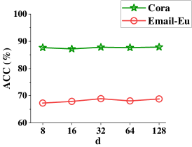
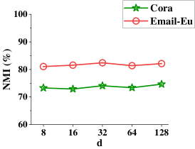
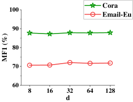
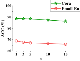
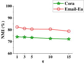
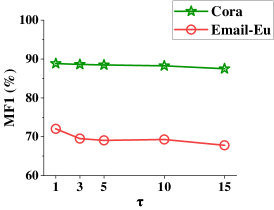
Figure 4: Sensitivity analysis of hyperparameters ($d,\tau$).

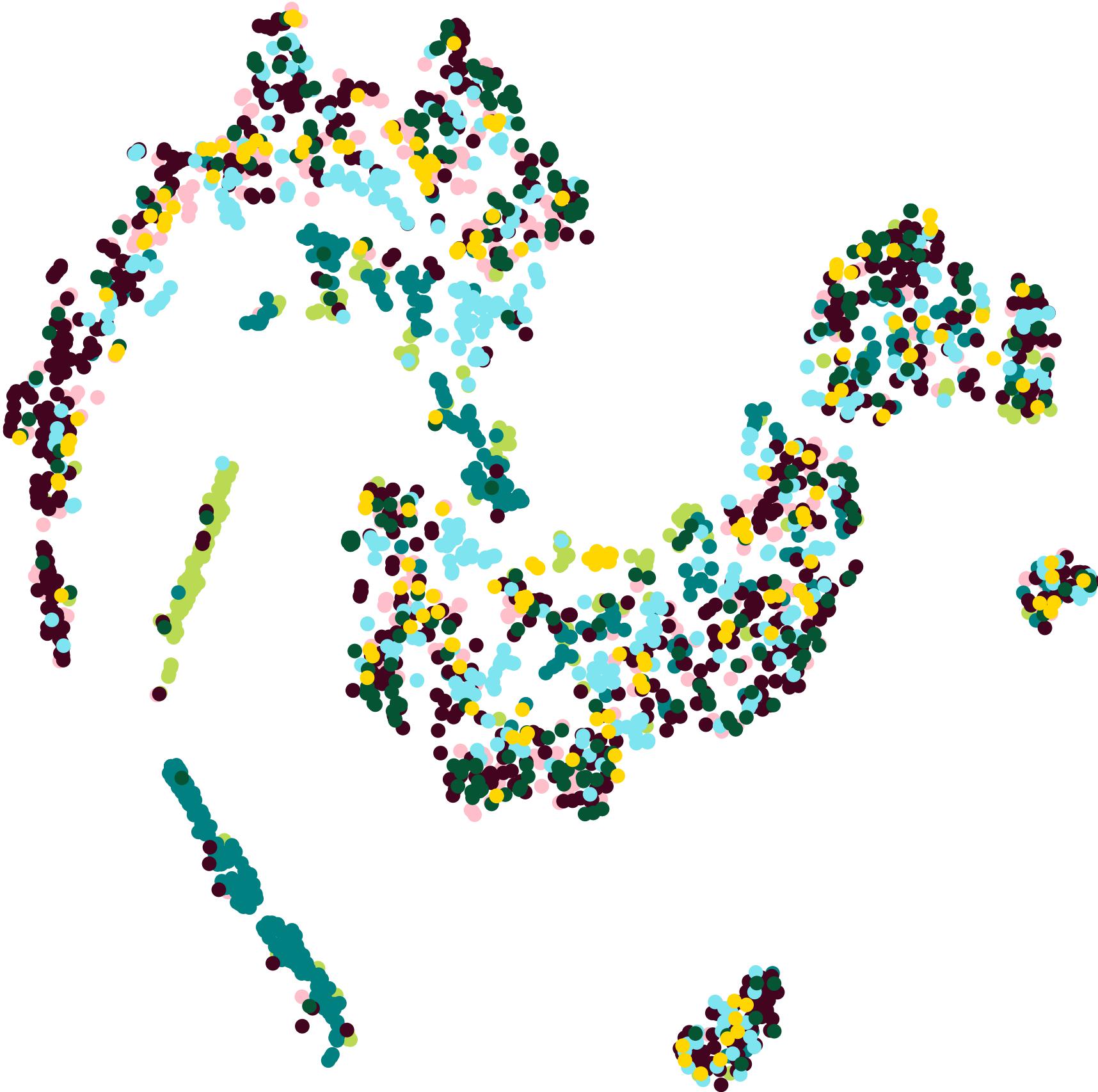
(a) $\varepsilon$=10

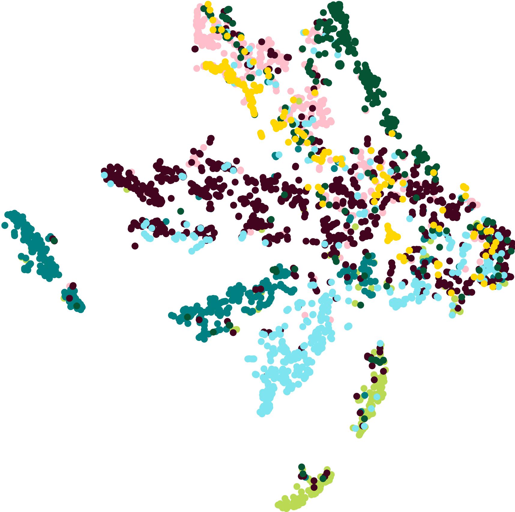
(b) $\varepsilon$=30

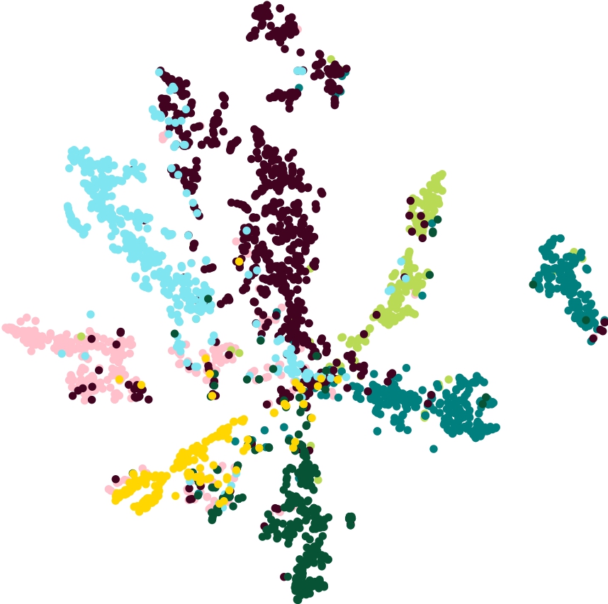
(c) $\varepsilon$=500

Figure 5: Community detection performance on Cora.

V-E The Case Study

We evaluated the community detection performance of the GCLS² model on Cora by the T-SNE [35] downscaling. Specifically, after the training of Algorithm 1 for $\varepsilon$ = {10, 30, 500}, respectively, we visualized the distribution of node features $Z$ in two dimensions, using nodes in 7 different colors to represent the 7 communities. The results are shown in Figure 5. We can clearly see that from $\varepsilon$ = 10 to 30 iterations, the labeled nodes are closing in on the communities corresponding to the labels. By 500 iterations, the detection accuracy is significantly improved, validating the effectiveness of our GCLS² model.

VI Conclusion

In this paper, we analyze the limitations of traditional GCL methods for community detection, and propose a novel Graph Contrastive Learning with Structure Semantics (CGLS²) framework for the community detection. We construct a high-level structure view based on classical community structure, and then extract structural and attribute semantics through the structure similarity semantics encoder to obtain a comprehensive node feature representation. We also design the structure contrastive learning to enhance the structural feature representation of nodes for more accurate community detection. Extensive experiments confirm the effectiveness of our GCLS² approach.

References

- [1] J. C. Whisstock and A. M. Lesk, “Prediction of protein function from protein sequence and structure,” Quarterly Reviews of Biophysics, vol. 36, no. 3, pp. 307–340, 2003.
- [2] P. Bedi and C. Sharma, “Community detection in social networks,” Wiley Interdisciplinary Reviews: Data Mining and Knowledge Discovery, vol. 6, no. 3, pp. 115–135, 2016.
- [3] F. Liu, S. Xue, J. Wu, C. Zhou, W. Hu, C. Paris, S. Nepal, J. Yang, and P. S. Yu, “Deep learning for community detection: Progress, challenges and opportunities,” in Proceedings of the International Joint Conference on Artificial Intelligence, (IJCAI), 2020, pp. 4981–4987.
- [4] M. R. Keyvanpour, M. B. Shirzad, and M. Ghaderi, “Ad-c: A new node anomaly detection based on community detection in social networks,” International Journal of Electronic Business, vol. 15, no. 3, pp. 199–222, 2020.
- [5] F. D. Zarandi and M. K. Rafsanjani, “Community detection in complex networks using structural similarity,” Physica A: Statistical Mechanics and its Applications, vol. 503, pp. 882–891, 2018.
- [6] A. A. Amini, A. Chen, P. J. Bickel, and E. Levina, “Pseudo-likelihood methods for community detection in large sparse networks,” The Annals of Statistics, pp. 2097–2122, 2013.
- [7] Z. Li and J. Liu, “A multi-agent genetic algorithm for community detection in complex networks,” Physica A: Statistical Mechanics and its Applications, vol. 449, pp. 336–347, 2016.
- [8] Z. Chen, L. Li, and J. Bruna, “Supervised community detection with line graph neural networks,” in International Conference on Learning Representations (ICLR), 2019.
- [9] X. Xin, C. Wang, X. Ying, and B. Wang, “Deep community detection in topologically incomplete networks,” Physica A: Statistical Mechanics and its Applications, vol. 469, pp. 342–352, 2017.
- [10] K. He, H. Fan, Y. Wu, S. Xie, and R. Girshick, “Momentum contrast for unsupervised visual representation learning,” in Proceedings of the IEEE/CVF Conference on Computer Vision and Pattern Recognition, 2020, pp. 9729–9738.
- [11] Y. Zhu, Y. Xu, F. Yu, Q. Liu, S. Wu, and L. Wang, “Deep Graph Contrastive Representation Learning,” in ICML Workshop on Graph Representation Learning and Beyond, 2020.
- [12] ——, “Graph contrastive learning with adaptive augmentation,” in Proceedings of the Web Conference (WWW), 2021, pp. 2069–2080.
- [13] Y.-X. Kong, G.-Y. Shi, R.-J. Wu, and Y.-C. Zhang, “k-core: Theories and applications,” Physics Reports, vol. 832, pp. 1–32, 2019.
- [14] X. Huang, H. Cheng, L. Qin, W. Tian, and J. X. Yu, “Querying k-truss community in large and dynamic graphs,” in Proceedings of the ACM SIGMOD International Conference on Management of Data (SIGMOD), 2014, pp. 1311–1322.
- [15] E. Gregori, L. Lenzini, and S. Mainardi, “Parallel k-clique community detection on large-scale networks,” IEEE Transactions on Parallel and Distributed Systems, vol. 24, no. 8, pp. 1651–1660, 2012.
- [16] A. Lancichinetti and S. Fortunato, “Community detection algorithms: a comparative analysis,” Physical Review E—Statistical, Nonlinear, and Soft Matter Physics, vol. 80, no. 5, p. 056117, 2009.
- [17] X. Jian, X. Lian, and L. Chen, “On efficiently detecting overlapping communities over distributed dynamic graphs,” in International Conference on Data Engineering (ICDE). IEEE, 2018, pp. 1328–1331.
- [18] T. N. Kipf and M. Welling, “Semi-supervised classification with graph convolutional networks,” in International Conference on Learning Representations (ICLR), 2017.
- [19] P. Veličković, G. Cucurull, A. Casanova, A. Romero, P. Liò, and Y. Bengio, “Graph attention networks,” in International Conference on Learning Representations (ICLR), 2018.
- [20] P. Veličković, W. Fedus, W. L. Hamilton, P. Liò, Y. Bengio, and R. D. Hjelm, “Deep graph infomax,” in International Conference on Learning Representations (ICLR), 2018.
- [21] K. Hassani and A. H. Khasahmadi, “Contrastive multi-view representation learning on graphs,” in International Conference on Machine Learning (ICML). PMLR, 2020, pp. 4116–4126.
- [22] X. Shen, D. Sun, S. Pan, X. Zhou, and L. T. Yang, “Neighbor contrastive learning on learnable graph augmentation,” in Proceedings of the AAAI Conference on Artificial Intelligence (AAAI), 2023, pp. 9782–9791.
- [23] Y. Ye, X. Lian, and M. Chen, “Efficient exact subgraph matching via gnn-based path dominance embedding,” Proceedings of the VLDB Endowment, vol. 17, no. 7, 2024.
- [24] N. Rai and X. Lian, “Top- community similarity search over large-scale road networks,” IEEE Transactions on Knowledge and Data Engineering, vol. 35, no. 10, pp. 10 710–10 721, 2023.
- [25] M. C. Frith, L. Noé, and G. Kucherov, “Minimally overlapping words for sequence similarity search,” Bioinformatics, vol. 36, no. 22-23, pp. 5344–5350, 2020.
- [26] Y. Zhao, H. Tang, and Y. Ye, “Rapsearch2: a fast and memory-efficient protein similarity search tool for next-generation sequencing data,” Bioinformatics, vol. 28, no. 1, pp. 125–126, 2012.
- [27] J. Yang and J. Leskovec, “Defining and evaluating network communities based on ground-truth,” in Proceedings of the ACM SIGKDD Workshop on Mining Data Semantics, 2012, pp. 1–8.
- [28] L. Chang, M. Xu, and D. Strash, “Efficient maximum k-plex computation over large sparse graphs,” Proceedings of the VLDB Endowment, vol. 16, no. 2, pp. 127–139, 2022.
- [29] P. Sen, G. Namata, M. Bilgic, L. Getoor, B. Galligher, and T. Eliassi-Rad, “Collective classification in network data,” AI Magazine, vol. 29, no. 3, pp. 93–93, 2008.
- [30] O. Shchur, M. Mumme, A. Bojchevski, and S. Günnemann, “Pitfalls of graph neural network evaluation,” arXiv preprint arXiv:1811.05868, 2018.
- [31] H. Yin, A. R. Benson, J. Leskovec, and D. F. Gleich, “Local higher-order graph clustering,” in Proceedings of the International Conference on Knowledge Discovery and Data Mining (SIGKDD). ACM, 2017, pp. 555–564.
- [32] Y. Mo, L. Peng, J. Xu, X. Shi, and X. Zhu, “Simple unsupervised graph representation learning,” in Proceedings of the AAAI Conference on Artificial Intelligence (AAAI), 2022, pp. 7797–7805.
- [33] J. Chen and G. Kou, “Attribute and structure preserving graph contrastive learning,” in Proceedings of the AAAI Conference on Artificial Intelligence (AAAI), 2023, pp. 7024–7032.
- [34] D. Kong, C. Ding, and H. Huang, “Robust nonnegative matrix factorization using l21-norm,” in Proceedings of the ACM International Conference on Information and Knowledge Management, 2011, pp. 673–682.
- [35] L. Van der Maaten and G. Hinton, “Visualizing data using t-sne.” Journal of Machine Learning Research, vol. 9, no. 11, 2008.