Pathways from nucleation to raindrops.
Abstract
Cloud droplets grow via vapor condensation and collisional aggregation. Upon reaching approximately , their inertia allows them to capture smaller droplets during descent, initiating rain. Here, we show that raindrop formation is not primarily governed by gravity or thermal diffusion, but by a critical range of drop sizes () where collisions are largely ineffective and controlled by van der Waals and electrostatic interactions. We identify four pathways to rain. The coalescence pathway, which is slow, involves the broadening of the drop size distribution across the low-efficiency gap through collisions, until enough large individual droplets achieving efficient collisions have formed. The mixing pathway, which is faster, requires mixing at the cloud top with drop-free, cold, humid air to create locally supersaturated conditions that grow droplets above the low-efficiency gap. The electrostatic pathway bypasses the gap through a static vertical field creating attractive interactions between droplets. The turbulence pathway relies on air turbulence to bring the droplets together at an increased rate, but we show that this pathway is unlikely. For all dynamical mechanisms, we demonstrate that the initiation time for rainfall occurs at the crossover between the broadening of the drop size distribution and the emergence of individual droplets large enough to trigger the onset of the rainfall cascade.
I Introduction
I.1 Clouds and global warming
Anthropogenic climate change is a pressing issue that requires urgent attention and action [1]. The complexity of the problem arises from the intricate interplay between human activities and natural phenomena across a broad range of spatial and temporal scales. Among the various components of the Earth’s climate system, clouds play a pivotal role in regulating precipitation patterns, water resources, and agriculture. Moreover, clouds exhibit radiative effects that can vary depending on their geometry, clustering, and altitude [2]. Despite the overwhelming evidence for global warming, predicting its consequences on regional to global scales and the system’s responses to potential mitigation or adaptation efforts remains challenging.
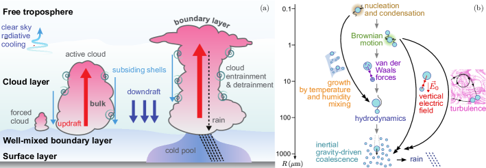
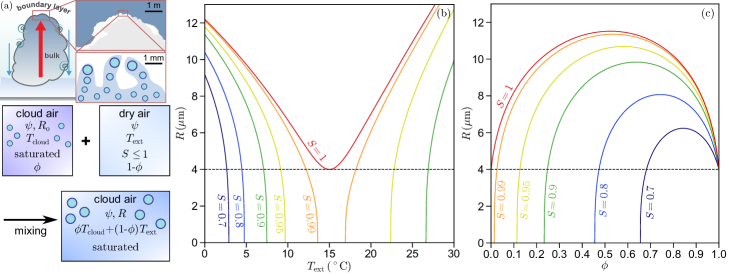
One of the significant sources of uncertainty in climate projections is the response of clouds to warming [3, 4, 5, 6]. Warm trade wind cumulus and stratocumulus clouds, which are prevalent in the subtropics, have a substantial impact on the global planetary albedo. These clouds are highly reflective and can cool the Earth’s surface by reflecting a significant amount of incoming solar radiation [7]. On the other hand, deep convective clouds, which are common in the tropics, can affect the atmospheric energy balance, circulation, and precipitation patterns. The behavior of these clouds under global warming is critical for understanding and predicting the Earth’s energy budget, hydrological cycle, and climate sensitivity [8, 9, 10, 11]. The atmosphere can be conceptualized as having a four-layer structure in the lowest portion of the troposphere (Fig. 1). The surface layer, where thermals, i.e. hot, humid, buoyant parcels form, is characterized by strong temperature gradients and turbulent mixing. Above the surface layer, a well-mixed convective layer is present, which is in the ultimate convective turbulent regime [12]. Forced, passive clouds form at the top of thermals, above the condensation level. This layer interacts with the weakly stratified cloud layer, where the convective ascent of active clouds is partly driven by latent heat exchange during condensation and evaporation processes. This layer is characteristic of cumulus-type clouds. In its absence, clouds rise within a background of turbulent convection, rather than within a stably stratified background, which is characteristic of stratocumulus clouds. Finally, the cloud layer is capped by a temperature inversion, inhibiting the ascent of clouds that would rise to this altitude and exhibiting significant radiative cooling. The strongly stratified free troposphere sits above this capping layer. This vertical structure determines the fate of a moist, buoyant parcel rising from the surface layer that could form a cloud and initiate rain. First, the parcel encounters colder air above it through the mixing layer, enhancing its updraft. In the cloud layer, latent heat release through condensation warms the parcel so that its top stays hotter than the surrounding air and keeps rising. Once it reaches the inversion, the parcel becomes capped by warmer air and stops ascending.
I.2 Warm clouds
In warm clouds, where ice is absent, the formation of droplets occurs on solid particles known as cloud condensation nuclei (CCN), as moist air ascends via convection and reaches the condensation level. The concentration of CCN can significantly impact the number and size of cloud droplets, which in turn can affect the cloud’s radiative properties and precipitation potential. The growth of these droplets via condensation ceases when the surrounding air becomes saturated [15, 16]. To better understand this process, let us consider droplets within a closed, isothermal system, assumed to be well-mixed. This system initially contains a certain number of soluble nuclei per unit volume, denoted as , and a supersaturated water vapor density, denoted as . The mass growth rate of a droplet of radius condensing in an atmosphere with vapor density is given by [17, chap. 13]:
| (1) |
Here, represents the density of liquid water, and is an effective diffusion coefficient of water molecules in air. Assuming that all droplets per unit volume have the same radius, the water vapor density can be expressed as , where is the water liquid density. The evolution equation governing the drop size can then be rewritten as:
| (2) |
In this equation, is the equilibrium radius determined by mass conservation, given by
| (3) |
As a consequence, the volume fraction of liquid water in clouds, typically less than , is thermodynamically controlled by the difference between and . is a characteristic growth time defined as:
| (4) |
This results in a trade-off between the typical drop size and the number of drops per unit volume. A higher concentration of condensation nuclei favors a large number of small drops over a small number of large drops [18]. The number of drops per unit volume in warm clouds is typically around , leading to micron-sized droplets as a result of condensation growth [19]. In clouds, is on the order of , and is in the range of to , resulting in ranging from seconds to minutes.
Cloud models, as well as weather and climate models, typically include a set of equations derived from thermofluidic equations, such as mass, momentum, and energy conservation. In this context, the droplet size distribution is a function of droplet size, space, and time. While some models directly solve the evolution equation of the distribution, allowing its shape to be obtained without imposing it a priori [20, 21, 22, 23] these methods can be numerically costly for simulated domains exceeding a few kilometers [24]. To solve larger domains, including some climate models, bulk parameterization schemes divide the size distribution into a few classes [25, 26, 6]. Based on the work of Kessler [27] and Berry and Reinhardt [28], two drop populations are typically considered: cloud drops and raindrops, with a separation around . Each class is represented by a small number of its moments, typically concentration and total mass. Transition rates between classes are then introduced phenomenologically, including autoconversion (cloud droplets becoming rain), accretion (rain droplets collecting cloud droplets), and autocollection (rain droplets collecting rain droplets) [27, 29, 30, 31, 32]. Some recent models simulate a small number of representative ”super-droplets” in a Lagrangian description to avoid the cost of an Eulerian description of the droplet field [33, 34, 35]. However, in all cases, the aggregation coefficients still need to be calculated a priori with good mechanistic knowledge of the processes involved to accurately describe the microphysics at the population level. For example, the collision rates between two cloud drops reported in the literature are sometimes inconsistent and calculated over narrow size ranges, leading to poorly resolved crossovers between different mechanisms [20].
I.3 Rain formation
Rain formation in warm clouds is a complex dynamic process that remains an active research topic in atmospheric sciences. The initiation of rain in warm clouds has been studied from two different perspectives in the literature. The first approach, proposed by Bowen [36], focuses on the growth of a single drop coalescing with a cloud of fixed droplets. The second approach involves numerically integrating the droplet distribution as a whole, which allows for the consideration of collective effects that can reduce the growth time [37, 28, 14]. Various explanatory mechanisms have been proposed to account for the observed dynamics of rain formation in warm clouds. These include stochastic effects of ”lucky drops” that are able to grow faster than their neighbors [38, 39], turbulence-induced rare but intense collisions [40, 41, 42, 43, 44, 45], the presence of giant condensation nuclei [46, 47, 48, 49], the break up of centimer-scale drops into smaller droplets [50, 51] and even radiative effects [52].
Despite these proposed mechanisms, the rapid appearance of rain within just to minutes in warm clouds remains largely unexplained and poses a significant challenge to understanding the underlying mechanisms [53]. One of the main complexities of rain formation in warm clouds is the vast separation between the concentration of raindrops and that of micron-sized droplets. The concentration of raindrops in clouds is typically smaller than that of the smaller droplets [54]. Due to this substantial size difference, rain in warm clouds must be formed through the collision and coalescence of cloud droplets. This process involves the merging of numerous droplets: one million droplets of radius are required to form a single millimeter-sized raindrop. Therefore, understanding the mechanisms behind the rapid appearance of rain in warm clouds remains an important research question in atmospheric physics.
Here, we propose a new method for mechanistically understanding the different contributions to growth towards rain. In Sec. II, we describe the mean-field coagulation equation modelling the evolution of the drop size distribution, the properties of the collision kernel describing collisions due to thermal diffusion and gravity, taking into account inertial effects in the gas flow, non-continuum lubrication, flow inside the drops and electrostatic interactions, as well as the numerical integration scheme. We investigate in Sec. III the interplay between the various microphysical mechanisms and their effects on the drop population growth dynamics. Finally in Sec. IV, we discuss under which conditions rain can be initiated rapidly enough and which mechanisms are significant in this process. Given the structure of the collision kernel, we isolate four possible scenarios for rain formation in warm clouds.
II Model
II.1 Smulochowksi equation
The modeling of the coagulation of droplets in warm clouds is based on the Smoluchowski equation, which describes the evolution of an ensemble of drops uniformly distributed in space and growing through successive pair coalescence [55]. This non-linear, integro-differential partial differential equation is mathematically complex and requires the expression of coefficients that describe the transition from one size to another. Denoting by the density of drops of mass , this evolution equation reads [55]:
| (5) |
where is the collisional kernel [56, 57, 17, 58]. is the collision rate of a single drop of mass with the population of drops of size . However, there is considerable uncertainty as to the details of the processes involved, particularly for droplets of commensurable sizes between and . The droplet size distribution in clouds broadens over time as droplets grow [59], which initially involves the interaction of micron-sized droplets of similar sizes. Fogs exhibit similar behaviors, evolving over time through condensation and collision. Identifying the mechanism of droplet growth from observations remains an active research question [60]. The complexity of dynamic measurements of drop size distributions in situ and the difficulty of separating out microphysical processes make numerically integrated theoretical models an important means of understanding cloud physics.
II.2 Collisional kernel
The Smoluchowski equation (5) admits simple solutions when the kernel follows self-similarity relations, which are defined by two conditions. The first condition is the homogeneity property for all [61, 62, 63, 64]. The second condition is the asymptotic behavior which applies for and symmetrically when by interchanging and . These conditions are met by certain physically relevant kernels, as discussed in Appendix A. In this generic case, the distribution evolves regularly, with the largest drops growing according to power laws of time. However, this evolution lacks the distinctive characteristic of rain: the abrupt emergence of a few very large drops.
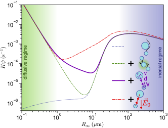
To elucidate the formation of rain, it is essential to account for the collective mechanisms governing the coalescence of drops of varying sizes, which renders the kernel not a homogeneous function. In the cloud physics literature, the nonhomogeneity effects in the kernel are typically represented by the collision efficiency , defined as the ratio between the full kernel and its asymptotic limit of ballistic gravity-driven collisions [65, 17]. In Ref. [66], we have extended this definition of the efficiency to include the small-size behavior of Brownian collisions in the asymptotic kernel. The complete kernel for two drops of radii , falling at their terminal velocities and diffusing with the diffusion coefficient , reads in this case
| (6) |
is a function of the Péclet number only, which quantifies the relative importance of diffusion and gravitational settling. When settling is much stronger than diffusion (), and the asymptotic kernel is purely ballistic. When diffusion is much stronger than settling (), , which corresponds to purely Brownian-driven collisions. In general, : the mechanisms creating nonhomogeneity in the kernel tend to inhibit collisions compared to idealized behaviors. However, as we shall see, it is not so much the value of the kernel that determines the growth dynamics, but rather its functional dependence with size.
The specifics of the kernel employed in this study are detailed in Ref. [66]. This kernel encompasses Brownian motion, droplet inertia, inertial effects in the gas flow, non-continuum lubrication, flow inside the drops, van der Waals interactions, and induced dipole forces in the presence of a static electric field. It also incorporates reference models for the effects of turbulence [45], which have a minor impact on the kernel under typical cloud conditions; their influence is discussed in Sec. IV. Figure 2 illustrates the collision rate of a single drop in a monodisperse spray of droplets with radius and number concentration , including a drop slightly larger than the spray droplets. The liquid water content is kept constant, causing to vary with as . The collision kernel exhibits two homogeneous asymptotic regimes. For small sizes below , Brownian diffusion dominates the collision rate. Collisions between droplets create a local concentration gradient, driving further collisions. Although larger droplets diffuse slower due to the Stokes-Einstein diffusion coefficient, their increased surface area allows for more collisions. These size dependencies balance each other, resulting in a homogeneity degree of in this regime so that decreases as . In the regime above , droplet inertia is large enough for them to fall in straight lines, overcoming the lubrication layer. The drag force on the droplets is also inertial, causing the terminal velocity to increase with their radius as . This results in a homogeneity degree of in this asymptotic regime. Contrary to conventional understanding, where the collision frequency transitions between a Brownian regime at small sizes and an inertial regime at large sizes [17], Fig. 2 reveals a range of drop sizes between and where both thermal diffusion and gravity are inefficient at inducing coagulation. The collision rate displays a minimum in this transitional regime. There is a small subregime between and where van der Waals interactions dominate the kernel. The attractive effect of these forces counteracts the repulsion of the lubrication layer, leading to an effective scaling law in this size range (for a more comprehensive discussion on this effect, see [66]). Around , the collision rate significantly increases with size as droplet inertia overcomes the lubrication layer. In this narrow subregime, the kernel loses all homogeneity. We therefore hypothesize that the sudden emergence of a few large drops and the transition to rain in warm clouds originate from the complex structure of the collision kernel.
II.3 Numerical integration
We revisit the problem of collisional aggregation of water droplets, considering the system at times larger than the condensation timescale . Drops are initially distributed at a size around , and the air between drops is saturated in water. A size-binning algorithm [67] is used to solve the Smoluchowski equation, dividing the drop size range into logarithmically distributed bins. Masses are expressed in units of the water molecule mass. The code is mass conservative. The transfer of mass between bins is computed using a quadratic interpolation of the mass density , biased in the direction of small masses. The scheme is upwind-biased and first order in time. The code has been validated on simple kernels leading to exact self-similar solutions, and on an exact solution derived for a particular kernel and initial solution [68] (see Supplementary Material). From the moments , the average drop mass describes the core of the distribution, and the tail is characterized by the typical drop mass . The initial number density of drops, , controlled by the density of nuclei is used to normalize the drop density so that the evolution depends on the initial shape of the distribution but not on the initial density , once time is rescaled by .
III Route to raindrops
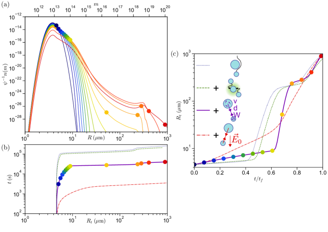
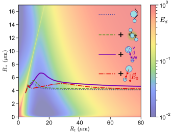
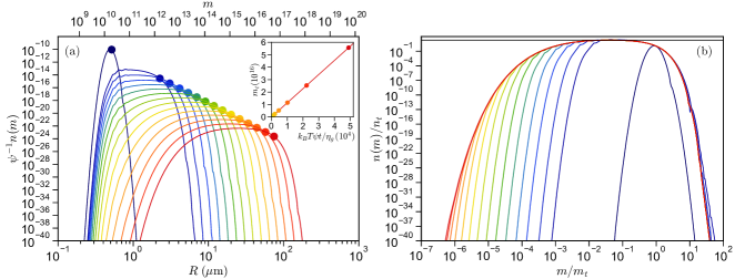
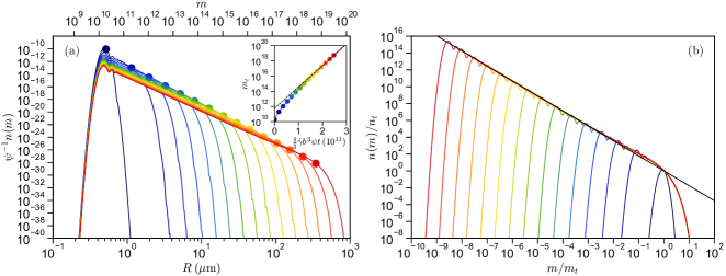
Figure 3 shows the typical time evolution of the drop density , starting from a ”cloud” of drops formed by condensation. Consistent with the collision rate shown in Fig. 2, the drop density evolves slowly until the tail starts presenting drops with a radius above . Drops larger than this cross-over size efficiently absorb smaller drops as they fall in the air due to their surface and inertia, accelerating their growth over a much shorter time-scale. Figure 3 shows this extremely rapid growth of the drops in the distribution tail once the low collision rate gap is crossed. To understand the statistical trajectory for the growth of drops across the low collision rate gap and the drop sizes involved in the coagulation process, we define the reaction mass as the mass for which half the collisions leading to a mass involve a small drop with a mass smaller than (see Appendix B for a formal definition). The reaction mass gives the typical size of the small drop involved in collisions producing drops of mass . This reaction size is shown for the typical size of drops in the distribution tails in Fig. 4. During the fast cascade producing raindrops, the most numerous collisions take place between the dominant species ( in the graph) and the largest drops. However, the situation is different during the crossing of the low collision rate gap, between to : the larger drops are formed by collisions inside the tails themselves, and not between drops in the tails and drops in the core of the distribution. This indicates that, despite drops larger than average being less numerous, the collision frequency is higher due to the sharp increase in collisional efficiency. The route to rain is therefore not controlled by a single dynamical mechanism that can easily be abstracted in an analytical model, but by subtle processes associated with the non-homogeneous structure of the collision kernel in the range of size surrounding the minimum of the collision efficiency.
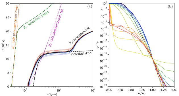
This result suggests a transition along the trajectory from nucleation to raindrops, shifting from a collective dynamics involving all possible collisions in the core of the distribution to a dynamics controlled by individual drops collecting mass while falling. Can these dynamics be described by low-dimensional models, such as the bulk parameterization schemes commonly used in cloud microphysics? To test this, we solve for the distribution using a reduced dimensionality model obtained by employing log-normal distributions as test functions. The equation is projected onto equations for the moments of the logarithm and . Figure 5 shows that this approximation quantitatively predicts the slow increase of the mean size at small sizes but fails to capture the cascade towards raindrops. Assuming that the few drops in the tail do not interact with each other, but only with the numerous small drops, we label each drop by a particular value of the cumulative distribution . Figure 5(b) shows that falls on a master curve when plotted as a function of the drop radius rescaled by a radius obtained at a reference value of (here chosen at ). This indicates that drops belonging to the distribution tail follow a similar path . Considering a single drop absorbing small drops distributed as predicted by the low dimensional model (bulk parametrization), its mass grows according to:
| (7) |
Figure 5(a) shows a good agreement at intermediate times when the mass contained in raindrops is negligible compared to the total mass. However, at longer times, the amount of small drops decreases due to their absorption by raindrops, leading to a new collective regime in which raindrops interact with each other indirectly through the depletion of the number of small drops.
IV Rain initiation time
IV.1 Coalescence pathway
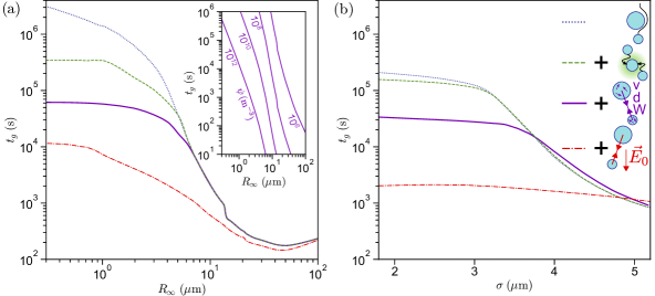
The first transition pathway to rain, starting from droplets of a few microns, involves the growth of droplets through coalescence. Figure 3 illustrates that the rain initiation time of this coalescence pathway to rain is directly determined by the time required for drops to grow across the low collision efficiency gap. This process is governed by the delicate balance between dynamical mechanisms persisting in the range of scales where both Brownian motion and inertia are small compared to other effects. Indeed, although collisions are driven by gravity and are limited by hydrodynamic effects, particularly by the lubrication layer, small effects, especially electrostatic ones, produce significant variations in efficiency. Figure 6(a) summarizes the dependence of the rain initiation time on the drop size . For comparison, in the context of a warm cumulus cloud, is observed to be on the order of [53, 14]. For this slow pathway to occur within a reasonably short time, enough droplets must be available for this nonlinear process to unfold rapidly enough. The rain initiation time is thus controlled by the liquid water content , as . Throughout this paper, the size of the initial distribution is varied while keeping a constant liquid water content, . This implies that larger initial drops are also less numerous. However, it is also feasible to vary the initial size for a given density, , which means that larger droplets also correspond to a larger liquid water content. For a given initial droplet size, , is given by . When is kept constant, is proportional to , which explains the rapid decrease of as size increases in this scenario. The curves of vs for any liquid water content can be obtained from Fig. 6(a) by shifting the curves vertically, towards larger times as decreases. Starting from a cloud composed of drops, one sees that would correspond to , which is far above any measured liquid water content. The insert in Fig. 6(a) presents the dependence of on the droplet density . The rain initiation is not only determined by but is also strongly influenced by the width of the initial distribution, as depicted in Fig. 6(b) using the standard deviation, . Notably, the presence of a few large droplets in the tail can initiate rain just as rapidly as increasing the average drop size.
IV.2 Mixing pathway
If the mean drop size exceeds , then Fig. 6(a) shows that the coalescence dynamics changes completely: the distribution contains drops large enough to enter the zone of efficient collisions, and the time becomes much less sensitive to the nature of the mechanisms determining the collision efficiency near its minimum. However, drops can hardly grow by condensation up to in the bulk of the cloud. We therefore hypothesize that the growth of drops across the collisional barrier takes place in the upper part of the cloud, where mixing with humid air at a different temperature can occur. This second transition pathway to rain thus involves creating particular conditions of saturation and CCN concentration above the cloud. To illustrate this fast mixing pathway to rain, we consider the isobaric mixing of a fraction of saturated air from the cloud with a fraction of dry, drop-free air [Fig. 7(a)]. Initially, the cloud air is at temperature and is saturated with a water vapor density . It contains a monodisperse population of droplets with number concentration and radius . The dry air above the cloud is at temperature and is subsaturated with a saturation , resulting in a water vapor density of . We assume that the density of cloud condensation nuclei (CCN) is the same inside and outside the cloud, leaving the cloud droplet concentration unchanged. The temperature and water vapor density after complete mixing are given by:
| (8) | ||||
| (9) |
We assume that the mixing process occurs on a timescale much shorter than the droplet condensation growth time. The mixing process can either create supersaturated conditions if , or evaporate droplets otherwise. Once condensation/evaporation has taken place, the final droplet size is given by Eq. (3):
| (10) |
Figure 7(b) shows the final size of droplets initially at , for a fixed mixing ratio . Above a threshold temperature of the air above the cloud, which increases with its saturation, droplets fully evaporate. If this air is wet and warm or cold enough, mixing leads to droplet growth. For given initial saturation and temperatures , , there is an optimal mixing ratio for droplet growth, as shown in Fig. 7(c). Mixing should incorporate enough dry air to create supersaturated conditions, but not so much that it dries out the upper part of the cloud. Mixing with colder air at the cloud top is only possible during the initial ascent of an air parcel, as it needs to be positively buoyant to find colder air above it. Once the cloud top reaches the inversion layer, it can no longer rise as it becomes capped by warmer air. However, the isobaric mixing process presented here is almost symmetrical with respect to which air volume is the warmest, as temperatures above in Fig. 7(b) show. Mixing with slightly subsaturated (, green curve) hot air can still lead to droplet growth, as long as it is warm enough. The conditions needed for growth above from this idealized mixing process alone are seldom fulfilled in clouds, requiring large temperature differences and very wet air above the cloud. Such conditions could be achieved by preconditioning of the atmosphere, through successive convective events that gradually moisten the air [69, 70, 71, 72].
IV.3 Electrostatic pathway
Going back to Fig. 3(b), one observes that van der Waals interactions between droplets results in a fivefold reduction in . This suggests a third possible pathway to rain. The gap in collision efficiency can be bypassed by the introduction of a static electric field large enough to close the low collision rate gap (dashed dotted red curve on Fig. 2). The typical field strength needed is (see [66]), which is significantly ( times) lower than the electric breakdown field of , leads to a further reduction in by a factor of . Figure 4 demonstrates that the collisional trajectory remains qualitatively consistent for all dynamical mechanisms considered. This consistency is reflected in the robust decomposition of the dynamics into a collective enlargement of the core of the distribution and individual drops growing in the tails by absorption of smaller drops. For drops on the order of , a rain initiation time requires an external electric field much larger than the values reported in the bulk of non-precipitating clouds [73, 74]. However, even if the bulk of the cloud is electrically neutral, the upper layer of the cloud may be subjected to significant electric fields. Recent observations and field campaigns have investigated the charge and electric fields of fair weather clouds, and has shown that in the midlatitudes, stratiform clouds are charged at cloud base [75, 76, 77]. The magnitude of these effects in the tropics is unclear [78, 79, 80, 81, 82]. Droplet charging, rather than the static vertical field presented here, could have effects on the droplet coalescence rate [83, 84]; however, droplets tend to have charges of the same sign, which creates repulsive interactions. Further work is needed to measure the electrical properties of clouds over their entire depth, along with their droplet populations, to determine which, if any, electrostatic mechanism could lead to increased collision rates.
IV.4 Turbulence pathway
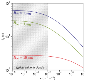
A fourth possible pathway for rain formation would be dominated by turbulence-induced collisions (Fig. 8). For particles smaller than the Kolmogorov length scale , which is the scale of the smallest turbulent structures, turbulence is known to increase collision rates through two different mechanisms. These effects are controlled by the turbulent Stokes number , where is the Stokes time of the particle with radius , and is the Kolmogorov time of the turbulent flow. At low , droplets follow the underlying flow and behave as passive tracers. When is large, the velocity fluctuates on timescales much shorter than the particle can respond to, allowing droplets to cross streamlines. is typically reached around . First, for moderate , particles cluster in regions of low vorticity, leading to enhanced collision rates. At larger , particles can be slung around by turbulent eddies and focused into regions where they meet with large relative velocities. A turbulent collision kernel has been proposed by Pumir and Wilkinson [45], based on the results of multiple direct numerical simulations of inertial particles in turbulence (see references therein). The total collision kernel is taken additively as a lowest-order approximation: . Here, refers to the kernel introduced previously, which accounts for Brownian motion, hydrodynamics, and van der Waals forces. For water droplets in air, turbulent coalescence dynamics are controlled only by the turbulent energy dissipation rate , typically around in clouds [85, 86]. Figure 8 shows that turbulence has little effect on the rain initiation time, due to the relatively weak turbulence in clouds. Its effect is larger for smaller drops, as the efficiency gap strongly decreases the Brownian-gravitational-electrostatic collision rate in this size range. Note that the turbulent collision efficiency is assumed to be unity, i.e., all hydrodynamic effects are neglected when the turbulent flow brings droplets together, and they are assumed to always coalesce. There is currently very little knowledge about the fine details of turbulence-induced collisions, which could, as is the case for gravitational collisions, strongly reduce the collision rate [87, 88, 89, 90, 91]. In the present stage of knowledge, this turbulence pathway to rain is unlikely in warm clouds.
V Conclusion
In conclusion, the initiation of rain in warm clouds requires two distinct conditions: the formation of rain precursors larger than in the upper part of the cloud, and the passage of these drops through a dense spray as they fall, allowing them to grow by collecting enough small drops (on the order of ). It is not the core of the drop size distribution that triggers the onset of this cascade, but rather its tails, which display much faster and very different dynamics. We have investigated four pathways in this article.
First, the coalescence pathway requires initially small droplets to cross the low-efficiency gap only by collision and coalescence, above which they rapidly grow. As the collision process is highly nonlinear, the time to go through this pathway is inversely proportional to the liquid water content. To account for the shortest observed rain initiation time (about ), this pathway requires large liquid water contents that may not be achieved in every precipitating cloud (roughly above ). However, many clouds can sustain themselves for much longer, typically a few hours, in which case this slow pathway becomes more likely.
Second, the mixing pathway bypasses the slow collision efficiency gap by growing droplets above through mixing of unsaturated, droplet-free air with wet, droplet-laden air at different temperatures at the cloud top. Mixing locally creates supersaturated conditions that grow existing droplets rather than nucleate new ones. This fast pathway depends on the local structure of the water vapor field and the drop size distribution [92, 93, 94, 69, 95, 96], and requires sufficiently wet air above the cloud to grow the droplets, rather than evaporate them and dry out the cloud. This suggests that the relative history of successive convective plumes would control rain initiation in this pathway. However, the temperature difference and humidity needed for droplet growth are large, and are unlikely to be realized in usual atmospheric conditions, at least for the mixing model presented here.
Third, the low-efficiency gap can be closed in the presence of a static vertical electric field inducing attractive electrostatic interactions between colliding droplets. This electrostatic pathway involves uncharged drops, as charged drops typically have the same charge [74], so their electrostatic interactions are repulsive, further increasing the rain formation time. The field strength needed for this pathway to become relevant is rather large (a fraction of the breakdown field), and has not been observed so far in warm precipitating clouds. In the absence of ice through which charges can be separated and large fields can emerge [97, 98, 99, 100, 101, 102], it is unclear how the required fields could be achieved.
Lastly, droplets can collide due to their relative velocities given by the underlying turbulence in clouds. If the droplets have sufficient inertia with regards to the fluctuations of this velocity field, their collision rate could be greatly enhanced. However, due to the relatively weak turbulence in clouds, this turbulence pathway is at this point very unlikely.
These four pathways are idealized scenarios that must now be tested using measurements performed in different types of clouds. We have identified here that droplet size distributions, liquid water content, electric field strengths, and turbulence intensities within various cloud environments should yield the most information on rain initiation. Additionally, large eddy simulations and cloud-resolving models [103] can help integrate these mechanisms and explore their interplay under different atmospheric conditions. By combining observations with the theoretical insights present here, we can achieve a better understanding of rain initiation processes and improve predictions of precipitation patterns. This multifaceted approach will not only enhance our fundamental knowledge of cloud physics but also contribute to more accurate weather forecasting and climate modeling.
Appendix A Self-similar kernels
Different kernels of physical interest present self-similar properties. The relative Brownian motion between two diffusing particles in a medium with viscosity results in a collision kernel, which has originally been studied by Smoluchowski [104]
| (11) |
Here, the exponents are and . Similarly, differential gravitational settling between two particles of radii , falling under their own weight at terminal velocity , results in the kernel:
| (12) |
There are two regimes for the fallspeed of droplets. At small Reynolds number (below in air), the drag on the droplets is governed by Stokes’ law, resulting in , and . At larger Reynolds number, the force on the droplets is quadratic with velocity so that , and . Lastly, in uniform shear flow at rate , the kernel is given by:
| (13) |
and , . This mechanism is relevant for small cloud droplets with low inertia, which collide due to local turbulent shear at sub-Kolmogorov scales [105]. For certain initial conditions and collision kernels, there are analytical solutions to the Smoluchowski equation. These include the constant kernel , the sum kernel and the product kernel [104, 106, 107, 108, 109]. However, only the constant kernel is of physical relevance, as it corresponds to the limit of the Brownian kernel where particles have the same size.
The values of the exponents , , control the qualitative behavior of the growth.
Figures 9(a) and 10(a) show the evolution of the distribution over time for two homogeneous kernels, respectively the Brownian kernel (11) and the shear kernel (13). With the Brownian kernel [Fig. 9(a)], the initially peaked distribution broadens and moves up in size, the typical size growing linearly in time. With the shear kernel [Fig. 10(a)], a power-law regime develops from the initial peak and grows towards larger sizes, and is cut off exponentially above . In both cases, after a short transient, the evolution enters a self-similar regime [Figs. 9(b) and 10(b)]: the rescaled distribution as a function of the rescaled size collapses onto the same curve at large , and extends over time as a power law towards smaller : for the Brownian kernel, ; for the shear kernel, . To understand these kinetics, we consider a single drop of mass , growing by collisions with drops per unit volume that are all of size . We assume that for all sizes, the scaling behavior holds exactly. The growth rate of the drop reads
| (14) |
Depending on the value of , three behaviors are possible. For , : the drop grows as a power law of time, linearly for Brownian motion (), as Fig. 9(a) shows. For , which is the case for the shear kernel, , as on Fig. 10(a). There is a remaining edge case: for , . diverges at finite time , which is unphysical. Actually, a solution exists at all times [110, 111, 112]. At the critical time , the dilute phase and its size distribution separate from a cluster of infinite size, referred to as a ”gel” by analogy with the gelation transition [113, 114, 115]. The finite gelation time obtained with these heuristics comes from finite size effects of the system; for and , the gelation time is rigorously zero [116]. It has been established that at long times, the size distribution no longer depends on the initial condition, but follows the scaling laws [117, 118, 61, 119]
| (15) |
is a constant and is a characteristic size of the system, e.g. the mean size , or a size constructed with higher order moments such as , used here. is a solution to the one-drop growth Eq. (14). Van Dongen and Ernst [119] have shown that the scaling function has two asymptotic regimes for . At large , , with a constant. At small , for – which is the case for the shear kernel – the scaling function follows a power law , as shown on Fig. 10(b). The exponent is smaller than and for , its value is set by the shape of ; here we find it to be around . For , decays exponentially at small , as Fig. 9(b) shows.
Appendix B Reaction trajectory
The growth term in the Smoluchowski equation (5) can be written as
| (16) |
by symmetry of the integrand around the axis . We are interested in the partial growth term
| (17) |
which describes the contribution of drops of size smaller than to the growth of drops of size . We define the reaction size as
| (18) |
In other words, the reaction size is the size for which the drops contribute half the growth rate of all the drops of sizes smaller than . The reaction size is defined with respect to another size; we take this size to be the typical size in the tails . The results shown here are not very sensitive to this choice, and are almost identical using instead the mean size .
is computed numerically in this paper, using the distributions obtained over time and the full expression of the kernel . To illustrate its physical meaning, we can compute it analytically in the ideal case of the constant kernel. For the kernel and an initial condition localized in mass space, the long-term behavior of the solution is [Eq. (15)]
| (19) |
The typical mass is . The partial growth rate is
| (20) |
such that the reaction size is
| (21) |
meaning that the droplets of typical size mostly react with each other. Numerically, we recover the prefactor at long times.
References
- Calvin et al. [2023] K. Calvin, D. Dasgupta, G. Krinner, A. Mukherji, P. W. Thorne, C. Trisos, J. Romero, P. Aldunce, K. Barrett, G. Blanco, W. W. Cheung, S. Connors, F. Denton, A. Diongue-Niang, D. Dodman, M. Garschagen, O. Geden, B. Hayward, C. Jones, F. Jotzo, T. Krug, R. Lasco, Y.-Y. Lee, V. Masson-Delmotte, M. Meinshausen, K. Mintenbeck, A. Mokssit, F. E. Otto, M. Pathak, A. Pirani, E. Poloczanska, H.-O. Pörtner, A. Revi, D. C. Roberts, J. Roy, A. C. Ruane, J. Skea, P. R. Shukla, R. Slade, A. Slangen, Y. Sokona, A. A. Sörensson, M. Tignor, D. Van Vuuren, Y.-M. Wei, H. Winkler, P. Zhai, Z. Zommers, J.-C. Hourcade, F. X. Johnson, S. Pachauri, N. P. Simpson, C. Singh, A. Thomas, E. Totin, P. Arias, M. Bustamante, I. Elgizouli, G. Flato, M. Howden, C. Méndez-Vallejo, J. J. Pereira, R. Pichs-Madruga, S. K. Rose, Y. Saheb, R. Sánchez Rodríguez, D. Ürge-Vorsatz, C. Xiao, N. Yassaa, A. Alegría, K. Armour, B. Bednar-Friedl, K. Blok, G. Cissé, F. Dentener, S. Eriksen, E. Fischer, G. Garner, C. Guivarch, M. Haasnoot, G. Hansen, M. Hauser, E. Hawkins, T. Hermans, R. Kopp, N. Leprince-Ringuet, J. Lewis, D. Ley, C. Ludden, L. Niamir, Z. Nicholls, S. Some, S. Szopa, B. Trewin, K.-I. Van Der Wijst, G. Winter, M. Witting, A. Birt, M. Ha, J. Romero, J. Kim, E. F. Haites, Y. Jung, R. Stavins, A. Birt, M. Ha, D. J. A. Orendain, L. Ignon, S. Park, Y. Park, A. Reisinger, D. Cammaramo, A. Fischlin, J. S. Fuglestvedt, G. Hansen, C. Ludden, V. Masson-Delmotte, J. R. Matthews, K. Mintenbeck, A. Pirani, E. Poloczanska, N. Leprince-Ringuet, and C. Péan, IPCC, 2023: Climate Change 2023: Synthesis Report. Contribution of Working Groups I, II and III to the Sixth Assessment Report of the Intergovernmental Panel on Climate Change [Core Writing Team, H. Lee and J. Romero (Eds.)]. IPCC, Geneva, Switzerland., Tech. Rep. (Intergovernmental Panel on Climate Change (IPCC), 2023).
- Tobin et al. [2012] I. Tobin, S. Bony, and R. Roca, Observational Evidence for Relationships between the Degree of Aggregation of Deep Convection, Water Vapor, Surface Fluxes, and Radiation, Journal of Climate 25, 6885 (2012).
- Bony et al. [2015] S. Bony, B. Stevens, D. M. W. Frierson, C. Jakob, M. Kageyama, R. Pincus, T. G. Shepherd, S. C. Sherwood, A. P. Siebesma, A. H. Sobel, M. Watanabe, and M. J. Webb, Clouds, circulation and climate sensitivity, Nature Geoscience 8, 261 (2015).
- Boucher et al. [2020] O. Boucher, J. Servonnat, A. L. Albright, O. Aumont, Y. Balkanski, V. Bastrikov, S. Bekki, R. Bonnet, S. Bony, L. Bopp, P. Braconnot, P. Brockmann, P. Cadule, A. Caubel, F. Cheruy, F. Codron, A. Cozic, D. Cugnet, F. D’Andrea, P. Davini, C. de Lavergne, S. Denvil, J. Deshayes, M. Devilliers, A. Ducharne, J.-L. Dufresne, E. Dupont, C. Éthé, L. Fairhead, L. Falletti, S. Flavoni, M.-A. Foujols, S. Gardoll, G. Gastineau, J. Ghattas, J.-Y. Grandpeix, B. Guenet, E. Guez, Lionel, E. Guilyardi, M. Guimberteau, D. Hauglustaine, F. Hourdin, A. Idelkadi, S. Joussaume, M. Kageyama, M. Khodri, G. Krinner, N. Lebas, G. Levavasseur, C. Lévy, L. Li, F. Lott, T. Lurton, S. Luyssaert, G. Madec, J.-B. Madeleine, F. Maignan, M. Marchand, O. Marti, L. Mellul, Y. Meurdesoif, J. Mignot, I. Musat, C. Ottlé, P. Peylin, Y. Planton, J. Polcher, C. Rio, N. Rochetin, C. Rousset, P. Sepulchre, A. Sima, D. Swingedouw, R. Thiéblemont, A. K. Traore, M. Vancoppenolle, J. Vial, J. Vialard, N. Viovy, and N. Vuichard, Presentation and Evaluation of the IPSL-CM6A-LR Climate Model, Journal of Advances in Modeling Earth Systems 12, e2019MS002010 (2020).
- Zhang and McFarlane [1995] G. Zhang and N. A. McFarlane, Sensitivity of climate simulations to the parameterization of cumulus convection in the Canadian climate centre general circulation model, Atmosphere-Ocean 33, 407 (1995).
- Schmidt et al. [2023] G. A. Schmidt, T. Andrews, S. E. Bauer, P. J. Durack, N. G. Loeb, V. Ramaswamy, N. P. Arnold, M. G. Bosilovich, J. Cole, L. W. Horowitz, G. C. Johnson, J. M. Lyman, B. Medeiros, T. Michibata, D. Olonscheck, D. Paynter, S. P. Raghuraman, M. Schulz, D. Takasuka, V. Tallapragada, P. C. Taylor, and T. Ziehn, CERESMIP: A climate modeling protocol to investigate recent trends in the Earth’s Energy Imbalance, Frontiers in Climate 5 (2023).
- Stevens et al. [2020] B. Stevens, S. Bony, H. Brogniez, L. Hentgen, C. Hohenegger, C. Kiemle, T. S. L’Ecuyer, A. K. Naumann, H. Schulz, P. A. Siebesma, J. Vial, D. M. Winker, and P. Zuidema, Sugar, gravel, fish and flowers: Mesoscale cloud patterns in the trade winds, Quarterly Journal of the Royal Meteorological Society 146, 141 (2020).
- Schneider et al. [2017] T. Schneider, J. Teixeira, C. S. Bretherton, F. Brient, K. G. Pressel, C. Schär, and A. P. Siebesma, Climate goals and computing the future of clouds, Nature Climate Change 7, 3 (2017).
- Stephens [1978] G. L. Stephens, Radiation Profiles in Extended Water Clouds. II: Parameterization Schemes, Journal of the Atmospheric Sciences 35, 2123 (1978).
- Bony et al. [2020] S. Bony, A. Semie, R. J. Kramer, B. Soden, A. M. Tompkins, and K. A. Emanuel, Observed Modulation of the Tropical Radiation Budget by Deep Convective Organization and Lower-Tropospheric Stability, AGU Advances 1, e2019AV000155 (2020).
- Muller et al. [2022] C. Muller, D. Yang, G. Craig, T. Cronin, B. Fildier, J. O. Haerter, C. Hohenegger, B. Mapes, D. Randall, S. Shamekh, and S. C. Sherwood, Spontaneous Aggregation of Convective Storms, Annual Review of Fluid Mechanics 54, 133 (2022).
- Ahlers et al. [2009] G. Ahlers, S. Grossmann, and D. Lohse, Heat transfer and large scale dynamics in turbulent Rayleigh-Bénard convection, Reviews of Modern Physics 81, 503 (2009).
- Bec [2005] J. Bec, Multifractal concentrations of inertial particles in smooth random flows, Journal of Fluid Mechanics 528, 255 (2005).
- Falkovich et al. [2006] G. Falkovich, M. G. Stepanov, and M. Vucelja, Rain Initiation Time in Turbulent Warm Clouds, Journal of Applied Meteorology and Climatology 45, 591 (2006).
- Twomey [1959] S. Twomey, The nuclei of natural cloud formation part II: The supersaturation in natural clouds and the variation of cloud droplet concentration, Geofisica Pura e Applicata 43, 243 (1959).
- Ghan et al. [2011] S. J. Ghan, H. Abdul-Razzak, A. Nenes, Y. Ming, X. Liu, M. Ovchinnikov, B. Shipway, N. Meskhidze, J. Xu, and X. Shi, Droplet nucleation: Physically-based parameterizations and comparative evaluation, Journal of Advances in Modeling Earth Systems 3, 10.1029/2011MS000074 (2011).
- Pruppacher and Klett [2010] H. Pruppacher and J. Klett, Microphysics of Clouds and Precipitation (Springer Netherlands, Dordrecht, 2010).
- Krueger [2020] S. K. Krueger, Technical note: Equilibrium droplet size distributions in a turbulent cloud chamber with uniform supersaturation, Atmospheric Chemistry and Physics 20, 7895 (2020).
- Hess et al. [1998] M. Hess, P. Koepke, and I. Schult, Optical Properties of Aerosols and Clouds: The Software Package OPAC, Bulletin of the American Meteorological Society 79, 831 (1998).
- Khain et al. [2000] A. Khain, M. Ovtchinnikov, M. Pinsky, A. Pokrovsky, and H. Krugliak, Notes on the state-of-the-art numerical modeling of cloud microphysics, Atmospheric Research 55, 159 (2000).
- Seifert et al. [2006] A. Seifert, A. Khain, A. Pokrovsky, and K. D. Beheng, A comparison of spectral bin and two-moment bulk mixed-phase cloud microphysics, Atmospheric Research 80, 46 (2006).
- Khain et al. [2015] A. P. Khain, K. D. Beheng, A. Heymsfield, A. Korolev, S. O. Krichak, Z. Levin, M. Pinsky, V. Phillips, T. Prabhakaran, A. Teller, S. C. Van Den Heever, and J.-I. Yano, Representation of microphysical processes in cloud-resolving models: Spectral (bin) microphysics versus bulk parameterization, Reviews of Geophysics 53, 247 (2015).
- Kreidenweis et al. [2019] S. M. Kreidenweis, M. Petters, and U. Lohmann, 100 Years of Progress in Cloud Physics, Aerosols, and Aerosol Chemistry Research, Meteorological Monographs 59, 11.1 (2019).
- Flossmann and Wobrock [2010] A. I. Flossmann and W. Wobrock, A review of our understanding of the aerosol–cloud interaction from the perspective of a bin resolved cloud scale modelling, Atmospheric Research From the Lab to Models and Global Observations: Hans R. Pruppacher and Cloud Physics, 97, 478 (2010).
- Cotton et al. [2011] W. R. Cotton, G. H. Bryan, and S. C. Van den Heever, Storm and Cloud Dynamics: The Dynamics of Clouds and Precipitating Mesoscale Systems, 2nd ed., International Geophysics Series No. 99 (Acad. Press, Amsterdam, 2011).
- Hansen et al. [2023] J. E. Hansen, M. Sato, L. Simons, L. S. Nazarenko, I. Sangha, P. Kharecha, J. C. Zachos, K. von Schuckmann, N. G. Loeb, M. B. Osman, Q. Jin, G. Tselioudis, E. Jeong, A. Lacis, R. Ruedy, G. Russell, J. Cao, and J. Li, Global warming in the pipeline, Oxford Open Climate Change 3, kgad008 (2023).
- Kessler [1969] E. Kessler, On the Distribution and Continuity of Water Substance in Atmospheric Circulations (American Meteorological Society, Boston, MA, 1969).
- Berry and Reinhardt [1974a] E. X. Berry and R. L. Reinhardt, An Analysis of Cloud Drop Growth by Collection Part II. Single Initial Distributions, Journal of the Atmospheric Sciences 31, 1825 (1974a).
- Berry and Reinhardt [1974b] E. X. Berry and R. L. Reinhardt, An Analysis of Cloud Drop Growth by Collection: Part IV. A New Parameterization, Journal of the Atmospheric Sciences 31, 2127 (1974b).
- Hall [1980] W. D. Hall, A Detailed Microphysical Model Within a Two-Dimensional Dynamic Framework: Model Description and Preliminary Results, Journal of the Atmospheric Sciences 37, 2486 (1980).
- Seifert and Beheng [2001] A. Seifert and K. D. Beheng, A double-moment parameterization for simulating autoconversion, accretion and selfcollection, Atmospheric Research 59–60, 265 (2001).
- Morrison et al. [2020] H. Morrison, M. van Lier-Walqui, A. M. Fridlind, W. W. Grabowski, J. Y. Harrington, C. Hoose, A. Korolev, M. R. Kumjian, J. A. Milbrandt, H. Pawlowska, D. J. Posselt, O. P. Prat, K. J. Reimel, S.-I. Shima, B. van Diedenhoven, and L. Xue, Confronting the Challenge of Modeling Cloud and Precipitation Microphysics, Journal of Advances in Modeling Earth Systems 12, e2019MS001689 (2020).
- Shima et al. [2009] S.-i. Shima, K. Kusano, A. Kawano, T. Sugiyama, and S. Kawahara, Super-Droplet Method for the Numerical Simulation of Clouds and Precipitation: A Particle-Based Microphysics Model Coupled with Non-hydrostatic Model, Quarterly Journal of the Royal Meteorological Society 135, 1307 (2009), arXiv:physics/0701103 .
- Grabowski et al. [2019] W. W. Grabowski, H. Morrison, S.-I. Shima, G. C. Abade, P. Dziekan, and H. Pawlowska, Modeling of Cloud Microphysics: Can We Do Better?, Bulletin of the American Meteorological Society 100, 655 (2019).
- Shima et al. [2020] S.-i. Shima, Y. Sato, A. Hashimoto, and R. Misumi, Predicting the morphology of ice particles in deep convection using the super-droplet method: Development and evaluation of SCALE-SDM 0.2.5-2.2.0, -2.2.1, and -2.2.2, Geoscientific Model Development 13, 4107 (2020).
- Bowen [1950] E. G. Bowen, The Fomation of Rain by Coalescence, Australian Journal of Chemistry 3, 193 (1950).
- Telford [1955] J. W. Telford, A New Aspect of Coalescence Theory, Journal of the Atmospheric Sciences 12, 436 (1955).
- Kostinski and Shaw [2005] A. B. Kostinski and R. A. Shaw, Fluctuations and Luck in Droplet Growth by Coalescence, Bulletin of the American Meteorological Society 86, 235 (2005).
- Wilkinson [2016] M. Wilkinson, Large Deviation Analysis of Rapid Onset of Rain Showers, Physical Review Letters 116, 018501 (2016).
- Ghosh et al. [2005] S. Ghosh, J. Dávila, J. Hunt, A. Srdic, H. Fernando, and P. Jonas, How turbulence enhances coalescence of settling particles with applications to rain in clouds, Proceedings of the Royal Society A: Mathematical, Physical and Engineering Sciences 461, 3059 (2005).
- Wilkinson et al. [2006] M. Wilkinson, B. Mehlig, and V. Bezuglyy, Caustic Activation of Rain Showers, Physical Review Letters 97, 048501 (2006).
- Wang and Grabowski [2009] L.-P. Wang and W. W. Grabowski, The role of air turbulence in warm rain initiation, Atmospheric Science Letters 10, 1 (2009).
- Devenish et al. [2012] B. J. Devenish, P. Bartello, J.-L. Brenguier, L. R. Collins, W. W. Grabowski, R. H. A. IJzermans, S. P. Malinowski, M. W. Reeks, J. C. Vassilicos, L.-P. Wang, and Z. Warhaft, Droplet growth in warm turbulent clouds, Quarterly Journal of the Royal Meteorological Society 138, 1401 (2012).
- Grabowski and Wang [2013] W. W. Grabowski and L.-P. Wang, Growth of Cloud Droplets in a Turbulent Environment, Annual Review of Fluid Mechanics 45, 293 (2013).
- Pumir and Wilkinson [2016] A. Pumir and M. Wilkinson, Collisional Aggregation Due to Turbulence, Annual Review of Condensed Matter Physics 7, 141 (2016).
- Szumowski et al. [1999] M. J. Szumowski, R. M. Rauber, and H. T. Ochs, The Microphysical Structure and Evolution of Hawaiian Rainband Clouds. Part III: A Test of the Ultragiant Nuclei Hypothesis, Journal of the Atmospheric Sciences 56, 1980 (1999).
- Mechem and Kogan [2008] D. B. Mechem and Y. L. Kogan, A Bulk Parameterization of Giant CCN, Journal of the Atmospheric Sciences 65, 2458 (2008).
- Posselt and Lohmann [2008] R. Posselt and U. Lohmann, Influence of Giant CCN on warm rain processes in the ECHAM5 GCM, Atmospheric Chemistry and Physics 8, 3769 (2008).
- Barahona et al. [2010] D. Barahona, R. E. L. West, P. Stier, S. Romakkaniemi, H. Kokkola, and A. Nenes, Comprehensively accounting for the effect of giant CCN in cloud activation parameterizations, Atmospheric Chemistry and Physics 10, 2467 (2010).
- Blanchard [1950] D. C. Blanchard, The behavior of water drops at terminal velocity in air, Transactions, American Geophysical Union 31, 836 (1950).
- Villermaux [2020] E. Villermaux, Fragmentation versus Cohesion, Journal of Fluid Mechanics 898, P1 (2020).
- Zeng [2018] X. Zeng, Modeling the Effect of Radiation on Warm Rain Initiation, Journal of Geophysical Research: Atmospheres 123, 6896 (2018).
- Beard and Ochs [1993] K. V. Beard and H. T. Ochs, Warm-Rain Initiation: An Overview of Microphysical Mechanisms, Journal of Applied Meteorology and Climatology 32, 608 (1993).
- McFarquhar [2022] G. M. McFarquhar, Rainfall microphysics, in Rainfall: Modeling, Measurement and Applications, edited by R. Morbidelli (Elsevier, 2022) pp. 1–26.
- von Smoluchowski [1916] M. von Smoluchowski, Three Presentations on Diffusion, Molecular Movement According to Brown and Coagulation of Colloid Particles., Physikalische Zeitschrift 17, 557 (1916).
- Gillespie [1972] D. T. Gillespie, The Stochastic Coalescence Model for Cloud Droplet Growth, Journal of the Atmospheric Sciences 29, 1496 (1972).
- Gillespie [1975] D. T. Gillespie, Three Models for the Coalescence Growth of Cloud Drops, Journal of the Atmospheric Sciences 32, 600 (1975).
- Khain and Pinsky [2018] A. P. Khain and M. Pinsky, Physical Processes in Clouds and Cloud Modeling, 1st ed. (Cambridge University Press, 2018).
- Brenguier and Chaumat [2001] J.-L. Brenguier and L. Chaumat, Droplet Spectra Broadening in Cumulus Clouds. Part I: Broadening in Adiabatic Cores, Journal of the Atmospheric Sciences 58, 628 (2001).
- Mazoyer et al. [2022] M. Mazoyer, F. Burnet, and C. Denjean, Experimental study on the evolution of droplet size distribution during the fog life cycle, Atmospheric Chemistry and Physics 22, 11305 (2022).
- Van Dongen [1987a] P. Van Dongen, Solutions of Smoluchowski’s coagulation equation at large cluster sizes, Physica A: Statistical Mechanics and its Applications 145, 15 (1987a).
- Aldous [1999] D. J. Aldous, Deterministic and stochastic models for coalescence (aggregation and coagulation): A review of the mean-field theory for probabilists, Bernoulli 5, 3 (1999).
- Fournier and Laurençot [2005] N. Fournier and P. Laurençot, Existence of Self-Similar Solutions to Smoluchowski’s Coagulation Equation, Communications in Mathematical Physics 256, 589 (2005).
- Herrmann et al. [2016] M. Herrmann, B. Niethammer, and J. J. L. Velázquez, Instabilities and oscillations in coagulation equations with kernels of homogeneity one, Quarterly of Applied Mathematics 75, 105 (2016).
- Langmuir [1948] I. Langmuir, The Production of Rain by a Chain Reaction in Cumulus Clouds at Temperatures Above Freezing, Journal of the Atmospheric Sciences 5, 175 (1948).
- Poydenot and Andreotti [2024] F. Poydenot and B. Andreotti, Gap in drop collision rate between diffusive and inertial regimes explains the stability of fogs and non-precipitating clouds, Journal of Fluid Mechanics 987, A37 (2024).
- Debry and Sportisse [2007] E. Debry and B. Sportisse, Solving aerosol coagulation with size-binning methods, Applied Numerical Mathematics 57, 1008 (2007).
- Golovin [1963] A. M. Golovin, The solution of the coagulation equation for cloud droplets in a rising air current, Izv. Geophys. Ser 5, 82 (1963).
- Roesner et al. [1990] S. Roesner, A. I. Flossmann, and H. R. Pruppacher, The effect on the evolution of the drop spectrum in clouds of the preconditioning of air by successive convective elements, Quarterly Journal of the Royal Meteorological Society 116, 1389 (1990).
- Hohenegger and Stevens [2013] C. Hohenegger and B. Stevens, Preconditioning Deep Convection with Cumulus Congestus, Journal of the Atmospheric Sciences 70, 448 (2013).
- Rapp et al. [2011] A. D. Rapp, C. D. Kummerow, and L. Fowler, Interactions between warm rain clouds and atmospheric preconditioning for deep convection in the tropics, Journal of Geophysical Research: Atmospheres 116, 10.1029/2011JD016143 (2011).
- Touzé-Peiffer et al. [2022] L. Touzé-Peiffer, R. Vogel, and N. Rochetin, Cold Pools Observed during EUREC4A: Detection and Characterization from Atmospheric Soundings, Journal of Applied Meteorology and Climatology 61, 593 (2022).
- Marshall et al. [1995] T. C. Marshall, M. P. McCarthy, and W. D. Rust, Electric field magnitudes and lightning initiation in thunderstorms, Journal of Geophysical Research: Atmospheres 100, 7097 (1995).
- Harrison et al. [2015] R. G. Harrison, K. A. Nicoll, and M. H. P. Ambaum, On the microphysical effects of observed cloud edge charging, Quarterly Journal of the Royal Meteorological Society 141, 2690 (2015).
- Nicoll and Harrison [2016] K. A. Nicoll and R. G. Harrison, Stratiform cloud electrification: Comparison of theory with multiple in-cloud measurements, Quarterly Journal of the Royal Meteorological Society 142, 2679 (2016).
- Harrison et al. [2017] R. G. Harrison, K. A. Nicoll, and K. L. Aplin, Evaluating stratiform cloud base charge remotely, Geophysical Research Letters 44, 6407 (2017).
- Harrison [2022] R. G. Harrison, Measuring electrical properties of the lower troposphere using enhanced meteorological radiosondes, Geoscientific Instrumentation, Methods and Data Systems 11, 37 (2022).
- Kartalev et al. [2006] M. D. Kartalev, M. J. Rycroft, M. Fuellekrug, V. O. Papitashvili, and V. I. Keremidarska, A possible explanation for the dominant effect of South American thunderstorms on the Carnegie curve, Journal of Atmospheric and Solar-Terrestrial Physics Vertical Coupling in the Atmosphere/Ionosphere System, 68, 457 (2006).
- Williams and Sátori [2004] E. R. Williams and G. Sátori, Lightning, thermodynamic and hydrological comparison of the two tropical continental chimneys, Journal of Atmospheric and Solar-Terrestrial Physics SPECIAL - Space Processes and Electrical Changes in Atmospheric L Ayers, 66, 1213 (2004).
- Williams [2009] E. R. Williams, The global electrical circuit: A review, Atmospheric Research 13th International Conference on Atmospheric Electricity, 91, 140 (2009).
- Harrison [2013] R. G. Harrison, The Carnegie Curve, Surveys in Geophysics 34, 209 (2013).
- Afreen et al. [2021] S. Afreen, N. J. Victor, S. Nazir, D. Siingh, G. Bashir, N. Ahmad, S. Javid Ahmad, and R. P. Singh, Fair-weather atmospheric electric field measurements at Gulmarg, India, Journal of Earth System Science 131, 7 (2021).
- Harrison et al. [2020] R. G. Harrison, K. A. Nicoll, M. H. P. Ambaum, G. J. Marlton, K. L. Aplin, and M. Lockwood, Precipitation Modification by Ionization, Physical Review Letters 124, 198701 (2020).
- Harrison et al. [2021] R. G. Harrison, K. A. Nicoll, D. J. Tilley, G. J. Marlton, S. Chindea, G. P. Dingley, P. Iravani, D. J. Cleaver, J. L. du Bois, and D. Brus, Demonstration of a Remotely Piloted Atmospheric Measurement and Charge Release Platform for Geoengineering, Journal of Atmospheric and Oceanic Technology 38, 63 (2021).
- Shaw [2003] R. A. Shaw, Particle-turbulence interactions in atmospheric clouds, Annual Review of Fluid Mechanics 35, 183 (2003).
- Mellado [2017] J. P. Mellado, Cloud-Top Entrainment in Stratocumulus Clouds, Annual Review of Fluid Mechanics 49, 145 (2017).
- Pinsky and Khain [1997a] M. B. Pinsky and A. P. Khain, Turbulence effects on the collision kernel. I: Formation of velocity deviations of drops falling within a turbulent three-dimensional flow, Quarterly Journal of the Royal Meteorological Society 123, 1517 (1997a).
- Pinsky et al. [1999] M. Pinsky, A. Khain, and M. Shapiro, Collisions of Small Drops in a Turbulent Flow. Part I: Collision Efficiency. Problem Formulation and Preliminary Results, Journal of the Atmospheric Sciences 56, 2585 (1999).
- Pinsky and Khain [1997b] M. B. Pinsky and A. P. Khain, Turbulence effects on droplet growth and size distribution in clouds—A review, Journal of Aerosol Science 28, 1177 (1997b).
- Ayala et al. [2008a] O. Ayala, B. Rosa, and L.-P. Wang, Effects of turbulence on the geometric collision rate of sedimenting droplets. Part 2. Theory and parameterization, New Journal of Physics 10, 075016 (2008a).
- Ayala et al. [2008b] O. Ayala, B. Rosa, L.-P. Wang, and W. W. Grabowski, Effects of turbulence on the geometric collision rate of sedimenting droplets. Part 1. Results from direct numerical simulation, New Journal of Physics 10, 075015 (2008b).
- Baker and Latham [1979] M. B. Baker and J. Latham, The Evolution of Droplet Spectra and the Rate of Production of Embryonic Raindrops in Small Cumulus Clouds, Journal of the Atmospheric Sciences 36, 1612 (1979).
- Baker et al. [1980] M. B. Baker, R. G. Corbin, and J. Latham, The influence of entrainment on the evolution of cloud droplet spectra: I. A model of inhomogeneous mixing, Quarterly Journal of the Royal Meteorological Society 106, 581 (1980).
- Baker et al. [1984] M. B. Baker, R. E. Breidenthal, T. W. Choularton, and J. Latham, The Effects of Turbulent Mixing in Clouds, Journal of the Atmospheric Sciences 41, 299 (1984).
- Villermaux et al. [2017] E. Villermaux, A. Moutte, M. Amielh, and P. Meunier, Fine structure of the vapor field in evaporating dense sprays, Physical Review Fluids 2, 074501 (2017).
- Allwayin et al. [2024] N. Allwayin, M. L. Larsen, S. Glienke, and R. A. Shaw, Locally narrow droplet size distributions are ubiquitous in stratocumulus clouds, Science 384, 528 (2024).
- Latham [1981] J. Latham, The electrification of thunderstorms, Quarterly Journal of the Royal Meteorological Society 107, 277 (1981).
- Williams et al. [1991] E. R. Williams, R. Zhang, and J. Rydock, Mixed-Phase Microphysics and Cloud Electrification, Journal of the Atmospheric Sciences 48, 2195 (1991).
- Saunders [1993] C. P. R. Saunders, A Review of Thunderstorm Electrification Processes, Journal of Applied Meteorology and Climatology 32, 642 (1993).
- Mason and Dash [2000] B. L. Mason and J. G. Dash, Charge and mass transfer in ice-ice collisions: Experimental observations of a mechanism in thunderstorm electrification, Journal of Geophysical Research: Atmospheres 105, 10185 (2000).
- Dash et al. [2001] J. G. Dash, B. L. Mason, and J. S. Wettlaufer, Theory of charge and mass transfer in ice-ice collisions, Journal of Geophysical Research: Atmospheres 106, 20395 (2001).
- Jungwirth et al. [2005] P. Jungwirth, D. Rosenfeld, and V. Buch, A possible new molecular mechanism of thundercloud electrification, Atmospheric Research 76, 190 (2005).
- Guichard and Couvreux [2017] F. Guichard and F. Couvreux, A short review of numerical cloud-resolving models, Tellus A: Dynamic Meteorology and Oceanography 69, 1373578 (2017).
- v Smoluchowski [1918] M. v Smoluchowski, Versuch einer mathematischen Theorie der Koagulationskinetik kolloider Lösungen, Zeitschrift für physikalische Chemie 92, 129 (1918).
- Saffman and Turner [1956] P. G. F. Saffman and J. S. Turner, On the collision of drops in turbulent clouds, Journal of Fluid Mechanics 1, 16 (1956).
- Davies et al. [1999] S. C. Davies, J. R. King, and J. A. D. Wattis, Self-similar behaviour in the coagulation equations, Journal of Engineering Mathematics 36, 57 (1999).
- Fernández-Díaz and Gómez-García [2007] J. M. Fernández-Díaz and G. J. Gómez-García, Exact solution of Smoluchowski’s continuous multi-component equation with an additive kernel, Europhysics Letters 78, 56002 (2007).
- Leyvraz [2003] F. Leyvraz, Scaling Theory and Exactly Solved Models In the Kinetics of Irreversible Aggregation, Physics Reports 383, 95 (2003).
- Krapivsky et al. [2010] P. L. Krapivsky, S. Redner, and E. Ben-Naim, A Kinetic View of Statistical Physics (Cambridge University Press, 2010).
- Leyvraz and Tschudi [1982] F. Leyvraz and H. R. Tschudi, Critical kinetics near gelation, Journal of Physics A: Mathematical and General 15, 1951 (1982).
- Ziff et al. [1983] R. M. Ziff, M. H. Ernst, and E. M. Hendriks, Kinetics of gelation and universality, Journal of Physics A: Mathematical and General 16, 2293 (1983).
- Ernst et al. [1984] M. Ernst, R. Ziff, and E. Hendriks, Coagulation processes with a phase transition, Journal of Colloid and Interface Science 97, 266 (1984).
- White [1980] W. H. White, A Global Existence Theorem for Smoluchowski’s Coagulation Equations, Proceedings of the American Mathematical Society 80, 273 (1980).
- White [1982] W. H. White, On the form of steady-state solutions to the coagulation equations, Journal of Colloid and Interface Science 87, 204 (1982).
- Lushnikov [2004] AA. Lushnikov, From sol to gel exactly, Physical Review Letters 93, 198302 (2004).
- Van Dongen [1987b] P. G. J. Van Dongen, On the possible occurrence of instantaneous gelation in Smoluchowski’s coagulation equation, Journal of Physics A: Mathematical and General 20, 1889 (1987b).
- Lushnikov [1973] AA. Lushnikov, Evolution of coagulating systems, Journal of Colloid and Interface Science 45, 549 (1973).
- van Dongen and Ernst [1985] P. G. J. van Dongen and M. H. Ernst, Dynamic Scaling in the Kinetics of Clustering, Physical Review Letters 54, 1396 (1985).
- Van Dongen and Ernst [1988] P. G. J. Van Dongen and M. H. Ernst, Scaling solutions of Smoluchowski’s coagulation equation, Journal of Statistical Physics 50, 295 (1988).