Action Gaps and Advantages in Continuous-Time Distributional Reinforcement Learning
Abstract
When decisions are made at high frequency, traditional reinforcement learning (RL) methods struggle to accurately estimate action values. In turn, their performance is inconsistent and often poor. Whether the performance of distributional RL (DRL) agents suffers similarly, however, is unknown. In this work, we establish that DRL agents are sensitive to the decision frequency. We prove that action-conditioned return distributions collapse to their underlying policy’s return distribution as the decision frequency increases. We quantify the rate of collapse of these return distributions and exhibit that their statistics collapse at different rates. Moreover, we define distributional perspectives on action gaps and advantages. In particular, we introduce the superiority as a probabilistic generalization of the advantage—the core object of approaches to mitigating performance issues in high-frequency value-based RL. In addition, we build a superiority-based DRL algorithm. Through simulations in an option-trading domain, we validate that proper modeling of the superiority distribution produces improved controllers at high decision frequencies.
1 Introduction
In many real-time deployments of reinforcement learning (RL)—quantitative finance, robotics, and autonomous driving, for instance—the state of the environment evolves continuously in time, but policies make decisions at discrete timesteps ( units of time apart) [28]. In such systems, the performance of value-based agents is sensitive to the frequency with which actions are taken. In particular, action values become indistinguishable as the time between actions decreases. In turn, in high-frequency settings, Baird demonstrated that action value estimates are susceptible to noise and approximation error [20]. Moreover, Tallec et al. exhibited that the performance of popular deep -learning agents is inconsistent and often poor [34].
In order to remedy this sensitivity, Baird proposed the advantage function and advantage-based variants of -learning, Advantage Updating (AU) [20] and Advantage Learning (AL) [2]. Unlike action values, advantages (appropriately rescaled) do not become indistinguishable as decision frequency increases. As a result, Baird, in [20, 2], demonstrated that advantage-based agents can learn faster and be more resilient to noise than their action value-based counterparts. Furthermore, Tallec et al., in [34], exhibited that their extension of AU, Deep Advantage Updating (DAU), works efficiently over a wide range of timesteps and environments, unlike standard deep -learning approaches.
While advantage-based approaches to RL have demonstrated robustness to decision frequency, in this work, we establish that they are nevertheless sensitive to the frequency with which actions are taken. This discovery arises as we answer the question: to what extent is the performance of distributional RL (DRL) agents sensitive to decision frequency? To this end, we build theory within the formalism of continuous-time RL where environmental dynamics are governed by SDEs, as in [25]. Additionally, we validate our theory empirically through simulations. Specifically, we make the following four contributions:
Distributional Action Gap. First, we extend notions of action gap to the realm of DRL. Precisely, we consider the minimal distance between pairs of action-conditioned distributions under metrics on the space of probability measures on . We observe that some metrics are viable for this extension, while others are not. This formalism sets the stage for analyzing the influence of individual actions as well as decision frequency on, for example, an agent’s return distributions.
Collapse of Distributional Control at High Frequency. Second, we establish tight bounds on the distributional action gaps of -dependent action-conditioned return distributions—return distributions induced by applying a specific initial action for units of time. We prove that these distributional action gaps not only collapse, as tends to zero, but do so at a slower rate than action-value gaps. On one hand, therefore, distributional -learning algorithms are susceptible to the same failures as -learning in continuous-time RL. On the other hand, however, remedies to these failures transliterated to distributional -learning algorithms are unlikely to succeed, because the means of these return distributions collapse faster than their other statistics.
Distributional Superiority. Third, we propose an axiomatic construction of a distributional analogue of the advantage, which we call the superiority. Leveraging our analysis of -dependent action-conditioned returns and their distributional action gaps, we present a frequency-scaled superiority distribution that enables greedy action selection at any fixed decision frequency.
A Distributional Action Gap-Preserving Algorithm. Fourth, we propose an algorithm that learns the superiority distribution from data. Empirically, we demonstrate that our algorithm maintains the ability to perform policy optimization at high frequencies more reliably than existing methods.
2 Setting
Notation: Spaces will either be subsets of Euclidean space or discrete. Measurability, in the former case, will be with respect to the Borel sigma algebra; in the latter case, it will be with respect to the power set. The set of probability measures over a space will be denoted by . Functions on spaces are assumed to be measurable. For and , the push forward of through/by , , is defined by . For a random variable , defined implicitly on some probability space , we write to denote the law of ; the notation is shorthand for . For any , the quantile function of , , is defined by , where is the CDF of .
2.1 Continuous-Time RL
Here we give a brief introduction to the technical aspects of continuous-time RL, à la [25]. We provide additional exposition and references in Appendix A. For any reader looking to defer some of this technical introduction, we summarize the core objects of interest at the end of Section 2.1.1.
2.1.1 MDPs
Continuous-time Markov Decision Processes (MDPs) are defined by three spaces and four measurable functions: a time interval with or with , a state space , an action space , a drift , a diffusion , a reward , and a terminal reward .111 We work with action-independent rewards. This is the norm in continuous-time DRL. The pair govern the environment’s dynamics by a family of SDEs parameterized by ,
| (2.1) |
Here is an -dimensional Brownian motion. In turn, any solution to (2.1) collects the state paths of an agent that chooses action at every time, regardless of the state they are in.
As is done in discrete-time RL, an agent might consider the induced Markov Reward Process (MRP) derived from a policy .222 We assume that is measurable for every and every . The dynamics of a policy-induced MRP (with policy ) are governed by the SDE
| (2.2) |
Here, following [38, 15, 16], the policy-averaged coefficients and are defined by
| (2.3) |
Thus, solutions to (2.2) collect the paths of an agent following policy .
A class of policies central to our study is those that fix an action from some time for a given persistence horizon .
Definition 2.1.
Given and , a policy is said to be -persistent at time if for all .
In particular, given a policy , we will consider -persistent modifications of : for ,
These policies will help us understand the influence of taking actions relative to others as well as to those taken by . We assume is small enough so that .
In order to guarantee the global-in-time existence and uniqueness of solutions to our SDEs (2.1) and (2.2), we make two sets of assumptions.
Assumption 2.2.
The functions and have linear growth and are Lipschitz in state, uniformly in time and action: a finite, positive constants exists such that
Assumption 2.3.
The averaged coefficient functions and are Lipschitz in state, uniformly in time: a finite, positive constant exists such that
These assumptions are standard in the analysis of continuous-time RL, optimal control, and SDEs [12, 26, 38, 16, 42]. Since is a function of state, we note that Assumption 2.3 is not a direct consequence of Assumption 2.2. The coefficients and satisfy the conditions of Assumption 2.3 provided and satisfy some (also standard) additional regularity conditions and satisfies some regularity conditions. These technical details are discussed in Appendix A.2.
In summary, in continuous-time RL, there are three stochastic processes of interest: with , all beginning at some time . These processes collect the state paths of an agent in one of three scenarios: 1. choosing action at every state and time; 2. following a policy ; or 3. choosing at every state and time for the first units of time and following thereafter.
2.1.2 Value Functions and their Distributions
Given a policy-induced state process , the (discounted) random return earned by starting from state at time is defined [41] by
| (2.4) |
where when . We distinguish returns earned by -persistent modifications of policies. We call these -dependent action-conditioned returns and denote them by . Given , they are defined by
| (2.5) |
Value-based approaches in RL estimate either the value function or the -dependent action-value function .333 In [38] and [16], the authors established and as continuous-time RL analogues of the classic value and action-value functions. We note, however, that this was done without explicitly defining and . As distributional approaches in RL estimate the laws of returns, following [41], we define
It is important to note that only the laws of random returns (and not their representations as random variables) are observable and modeled in practice.
2.2 -Learning in Continuous Time
The failure of action-value-based RL in continuous-time stems from the collapse of action values at a given state to the value of that state. Precisely, Tallec et al. and Jia and Zhou established that
| (2.6) |
where is independent of (see [34] and [16] respectively).444 The function is the Hamiltonian of the classic stochastic optimal control problem defined by our MDP. In a discrete action space, given a state and time , a concise way to capture the asymptotic information of (2.6) is by considering the action gap [11, 5] of the associated -dependent action values
Anticipating (2.6), which implies that , Baird proposed AU wherein he estimated the rescaled advantage function in place of :
| (2.7) |
Note that . Tallec et al. [34] and Jia and Zhou [16], following Baird, also estimated to ameliorate -learning in continuous time.
3 The Distributional Action Gap
In this section, we define a distributional notion of action gap; we prove that -dependent action-conditioned return distributions collapse to their underlying policy’s return distribution as vanishes; and we quantify the rate of collapse of these return distributions.
Definition 3.1.
Consider an MDP with discrete action space and let for a metric . The action gap of at a state and time is given by
While has a canonical metric, induced by , the space does not. So a choice must be made, and some metrics are unsuitable. For example, in deterministic MDPs with deterministic policies, return distributions are identified by expected returns: is the delta at , for all . Thus, should vanish as decreases to zero if vanishes as decreases to zero. With the total variation metric , for instance, this is not the case, making unsuitable. Indeed, suppose we have a deterministic MDP with and such that and , for some state and time (see, e.g., [34]). Then , for all , yet .
The distances from the theory of Optimal Transportation (see [36]), however, are suitable. They are defined via couplings of distributions.
Definition 3.2.
Let . A is a coupling of and if its first and second marginals are and respectively. We denote the set of these couplings by .
Definition 3.3.
Let 555 Here we assume that and have finite absolute th moments. and . The distance between and is
| (3.1) |
Any coupling attaining the infimum in (3.1) is called a -optimal coupling. Henceforth, we write when considering action gaps. If and are deltas at and respectively, then the right-hand side of (3.1) is equal to . Hence, in deterministic MDPs with deterministic policies, action gaps of are identical to action gaps of , making the distances suitable in the above sense. In non-deterministic MDPs, the relationship between and is opaque.
The following results study the action gap of as a function of , lending some color to the relationship between and . These results all hold under Assumptions 2.2 and 2.3. Henceforth, we suppress mention of these assumptions; we do not restate them explicitly. First, we observe that action gaps of are bounded from below by action gaps of . {restatable}propositiondistgapactiongap For all , we have that . For a proof of this statement and any other made in this work, see Appendix B. Our next result establishes that action gaps of , like action gaps of , vanishes for a large class of MDPs.
theoremvanishingwassersteingap If and are bounded, then , for all ; hence, .
While Theorem 3.3 shows that the distance between and (and the action gap of at ) does indeed vanish as decreases, it does not identify the rate at which it does so. Our next two theorems establish this rate.
theoremwitnesslargegap MDPs and policies exist in and under which, for all , we have that and .
Finally, we prove that for a large class of MDPs (different from but overlapping with the class of MDPs captured in Theorem 3.3), the lower bound found in Theorem 3.3 is an upper bound.
theoremwassersteinactiongapdecay If is Lipschitz in state, uniformly in time, is Lipschitz, and , then , for all ; hence, .
4 Distributional Superiority
In this section, we introduce a probabilistic generalization of the advantage. We define this random variable—which we call the superiority and denote by —via a pair of axioms.
A natural construction of the superiority at is given by . The law of this difference, however, depends on the joint law of , which is unobservable in practice and ill-defined (cf. Section 2.1.2). Yet, the set of all possible laws of this difference is easily characterized; it is the set of coupled difference representations of and .
Definition 4.1.
Let . A coupled difference representation (CDR) of and takes the form where and is given by . The set of all coupled difference representations of and will be denoted by .
Our first axiom places the superiority’s law in this set, .
Axiom 1.
The law of is a coupled difference representation of and .
Our second axiom encodes a type of consistency for deterministic policy behavior.
Axiom 2.
is deterministic whenever is -persistent at time .
To see how Axiom 2 encodes a notion of deterministic consistency, first consider its discrete-time analogue: the superiority at for a policy is deterministic if at deterministically chooses . In this situation, our -following agent makes the same choices as a -following agent—both take action in state initially and then follow thereafter—, and we posit that the superiority should not be random. The continuous-time analogue of the situation just described occurs precisely when a policy is -persistent at starting time . Given a starting time and state , an agent that chooses action between and and then follows is following the -persistent modification of at time . By definition, they make the same choices as a -following agent when is -persistent starting at time . Axiom 2 stipulates that, in this case, should be deterministic.
By construction, if , then its mean is (see Appendix B.2 for a proof of this claim). Axiom 2 then says that any determining coupling when is -persistent at time must be such that .666 Here ; so the mean of is . In particular, Axiom 2 nontrivially restricts .
Example 4.2.
Let for . If is -persistent at time , then . This variance is only when ’s return is deterministic. Hence, may be nontrivial even when conditioning on reflects the policy’s behavior exactly. We posit, via Axiom 2, that this should be prohibited.
In fact, Axiom 2 determines a single coupling, if we want a consistent choice across all time-state-action triplets and all MDPs. {restatable}theoremunqiuesuperiority Let for some . The push-forward of by is the delta at zero, , if and only if is a -optimal coupling, for some . Moreover, there is only one such coupling. It is given by or, equivalently, . Here is the uniform distribution on .
The second definition of corresponds, more generally, to the -optimal coupling, for all , of and given by . As ’s quanitle function is , we have in hand everything we need to define the superiority distribution (via its quantile function).
Definition 4.3.
The superiority distribution at is
As has the smallest possible central absolute th moments among all CDRs of and , heuristically, it captures more of the individual features of both return distributions than other such CDRs (like in Example 4.2). We illustrate this by example in Figure 4.1.
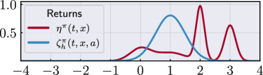 |
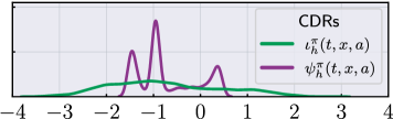 |
4.1 The Rescaled Superiority Distribution
From Section 3, we know that the distance between and , for every , vanishes as vanishes. Moreover, we know the rate at which this distance disappears. As a result, by construction, the central absolute th moments of collapse as collapses, and, for a large class of MDPs, we understand the rate at which these moments collapse. More generally and precisely, if we consider the -rescaled superiority distribution defined by
we see that Theorems 3.3 and 3.3 translate to the follow statements on action gaps of : {restatable}theoremrescaleddsuppreservelow MDPs and policies exist satisfying Assumptions 2.2 and 2.3 in and under which, for all , we have that . {restatable}theoremrescaleddsuppreserveup Under Assumptions 2.2 and 2.3, if is Lipschitz in state, uniformly in time, is Lipschitz, and , then , for all .
These two theorems tell us how to preserves the action gaps of -rescaled superiority distributions (as a function of ). They identify . For , action gaps vanish as vanishes. Whereas for , action gaps blow up as vanishes. These behaviors are undesirable. When , the influence of an action on an agent’s superiority becomes indistinguishable from any other action. For , ever larger sample sizes are need to obtain any statistical estimate of an agent’s superiority with the same level of accuracy. These scenarios are untenable.
Another consideration regarding rescalings of is whether they upend rankings of actions determined by some given measure of utility. This would be counterproductive. In DRL, agents often use distortion risk measures [1] to rank actions ([10, 9, 22, 4, 17]).
Definition 4.4.
Given , the distortion risk measure is defined by ; on , its value is given by the integral of with respect to .
A family of is the -conditional value-at-risk measures (-CVaR) [29], where for ; is the expected-value utility measure. Crucially, preserves -valued utility. {restatable}theoremrescaleddsuprank Let be a distortion risk measure, , and . If , then . In turn, the -rescaled superiority distribution is not only action gap preserving but matches in its greedy choice of action as measured by a distortion risk measure.
4.2 Algorithmic Considerations
We now turn to building DRL algorithms based on our theory. Our algorithms leverage the quantile TD-learning framework [10] to learn -greedy policies, for a given distortion risk measure , just as DAU [34] leverages the -learning framework to learn greedy policies. Full pseudocode and implementation details are given in Appendix C.
At the heart of our algorithms is an equality of quantile functions, which holds by construction,
| (4.1) |
Indeed, given and , as models of and respectively, equation (4.1) justifies the application of quantile TD-learning to , as a model for , defined via the quantile function
| (4.2) |
That said, we cannot realize quantile TD-learning without defining predictions and bootstrap targets in terms of -quantile representations777 An -quantile representation of a given distribution in is a vector in whose th component encodes the -quantile of said distribution. [10, 4] of via those of and .
While we may freely parameterize the -quantile representation of with a neural network (with interface) , we have to be careful when parameterizing the -quantile representation of . Given a neural network , we set
| (4.3) |
This ensures we identify a -greedy policy; it is at the -greedy action (cf. [34, Eq. 27]).
With appropriate parameterized -quantile representations of and in hand, we derive our predictions and bootstrap targets. By (4.2), recalling and (4.3), we compute our predictions via
| (4.4) |
By Wiltzer [40], as and , observe that
where 888 This holds if is continuous, a standard assumption in continuous-time control (see, e.g., [25, 34, 16]). for all . So upon getting a sample state/realization of , as in [30], we compute our bootstrap targets via
| (4.5) |
In summary, the predictions (4.4) and the bootstrap targets (4.5) together characterize a family of QR-DQN-based algorithms called DSUP(), whose core update is outlined in Algorithm 1.
One theoretical drawback of DSUP() for mean-return control is that the mean of the -rescaled superiority distribution is only when , by (2.6) and (2.7). Thus, we propose modeling simultaneously. This yields a novel form of a two-timescale approach to value-based RL (see, e.g., [8]). In particular, we estimate defined by
We call the advantage-shifted -rescaled superiority. Note that its mean is , which is . To realize this, we approximate using DAU and employ parameter sharing between the approximators of and . We call this family of algorithms DAU+DSUP(). We note that is used only for increasing action gaps; it does not change the training loss for and .
5 Simulations
The empirical work herein is two-fold in nature: illustrative and comparative. First, we simulate an example that illustrates Theorems 3.3/4.1 and Theorem 3.3/4.1 and their consequences. Second, in an option-trading environment, we compare the performance of -based agent(s) against QR-DQN [10] and DAU [34] in the risk-neutral setting and against QR-DQN in a risk-sensitive setting.
5.1 The Rescaled Superiority Distribution Revisited
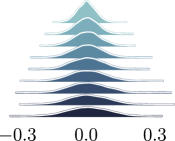
Consider an MDP with time horizon , a two element action space, and —when action is executed, the system follows -dimensional Brownian dynamics with a constant drift of , and otherwise, the state is fixed—, a reward that equals the agent’s signed distance to , and a trivial terminal reward. We estimate four distributions at for the policy that always selects . Figure 5.1 shows these estimated distributions for a sample of frequencies (kHz), .
 |
 |
 |
 |
First (from the left), we see that collapses to , as tends to . Thus, accurate action ranking distributional or otherwise becomes impossible in the vanishing limit. Second, we see that rescaling by produces distributions with mean but infinite non-mean statistics in the vanishing limit. Here the means are imperceptible in face of the large variances. So while this rescaling permits ranking actions by action values, it does so at the expense of producing high-variance distributions.
Third, we see that rescaling by yields distributions with non-mean statistics but vanishingly small means, . Hence, this rescaling permits ranking actions by non-mean statistics, even if action values again becomes indistinguishable in the vanishing limit. That said, the vanishing rate of the means here is slower than when no rescaling is considered, . Fourth, we see that rescaling by and then shifting it by produces distributions with mean and non-mean statistics. In turn, this two-timescale approach permits ranking actions by either action values or non-mean statistics (but not both by Theorem 4.4). However, the mean estimates here are inaccurate and imprecise—rather than uniformly being , they oscillate substantially.
In risk-neutral control, we are left with a number of questions. What effect do the high variance distributions in DAU/DSUP() have on performance? What effect do the means have on the performance of DSUP()? What effect does the instability of the mean estimates in DAU+DSUP() have on performance? In Section 5.2, we begin to answer these questions and others by testing our superiority-based algorithms against appropriate benchmarks in an option-trading environment.
5.2 High-Frequency Option Trading
The option-trading environment in which we run our comparative experiments is a commonly used benchmark (see, e.g., [22, 17]). We use an Euler–Maruyama discretization scheme [23] at high resolution to simulate high-frequency trading. Returns are averaged over seeds and different dynamics models (corresponding to data from different stocks). Additionally, following [22], we use disjoint datasets to estimate the dynamics parameters for simulation during training and evaluation.999 Our code is available at https://github.com/harwiltz/distributional-superiority.
First, we consider the risk-neutral setting. Here we compare QR-DQN, DAU, and three algorithms based on the -rescaled superiority distribution with : DSUP(), DAU+DSUP(), and DSUP(). Figure 5.2 summarizes their performance at a sample of frequencies (Hz).
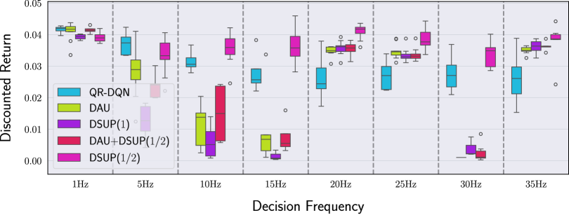
We see that DSUP() is not only the most consistent performer, but outperforms every competitor at all but the two lowest frequencies. Even then, its performance is very close to the best performer. We also see that DAU+DSUP()’s preservation of both action gaps and action gaps does not lead to the strongest performance. In particular, its performance is inconsistent and sometimes poor. We believe this is because the tested frequencies are low enough that DSUP() maintains large enough action gaps to learn performant policies, but high enough that the variances of the distributions underlying cause estimation difficulty. Indeed, the three methods that estimate (explicitly in DAU and DAU+DSUP() or implicitly in DSUP()) exhibit almost identical behavior.
Our results highlight a dichotomy in existing (ours included) methods for value-based, high-frequency, risk-neutral control. They can either maintain expected return estimates or return variance estimates, but not both. We observe better performance in estimating small means from variance distributions than in estimating means from receipricolly large variance distributions.
To qualitatively illustrate the appeal of the -rescaled superiority, Figure 5.3 presents examples of learned action-conditioned distributions used by DSUP() and QR-DQN agents to make decisions.
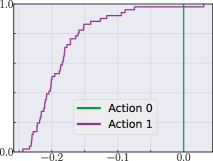
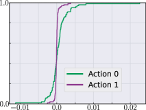
In this environment, action taken in the start state terminates the episode, yielding the smallest return, , making this action inferior to its alternative action, . We see that DSUP() infers this fact. QR-DQN, on the other hand, has difficulty distinguishing these actions. This is because the -rescaled superiority preserves action gaps, while does not.
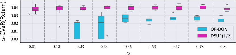
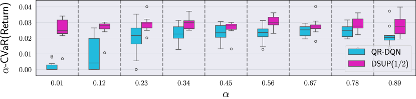
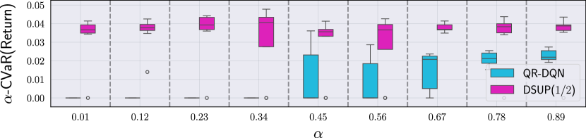
Second, we consider a risk-sensitive setting. Here we compare QR-DQN and DSUP() using -CVaR for greedy action selection. We do this because Theorem 4.4 does not hold with , and preserving means is less critical in risk-sensitive control than it is in risk-neutral control. Figure 5.4 depicts our results at (see Appendix D for results across a range of ).
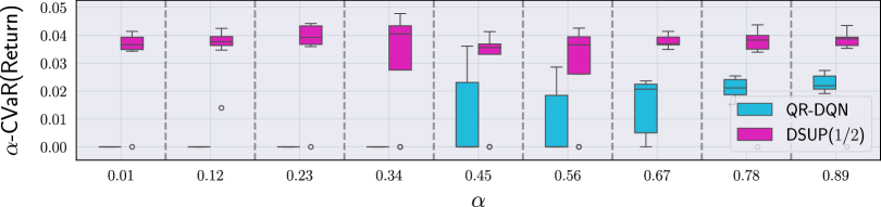
Again, we see that DSUP() is conclusively the best performer.
6 Related Work
Notions of action gap and ranking have long been of interest in RL (see, e.g., [11]). Action gaps are related to sample complexity in RL—indeed, instance-dependent sample complexity rates are inversely proportional to the divergence between action-conditioned return distributions ([13, 19, 37]). Bellemare et al. [5] argue for the consideration of alternatives to the Bellman operator that explicitly devalue suboptimal actions, and they show that Baird’s AL [2] operator falls within this class of operators. On the other hand, Schaul et al. [31] implicitly question Bellemare et al.’s position. They demonstrate that stochastic gradient updates in deep value-based RL algorithms induce frequent changes in relative action values, which in turn is a mechanism for exploration.
The advantage function is commonplace in RL (see, e.g., [39, 32, 27, 35, 24]). In [24], Mésnard et al. employ a distributional critic that is closely related to our (unscaled) distributional superiority. Their choice of critic stems from a desire to minimize variance. We note that the distributional superiority is a posteriori characterized as a minimal variance coupled difference representation of action-conditioned return distributions and policy-induced return distributions.
Lastly, DRL in continuous-time MDPs is in its infancy. There are only three works to mention. Wiltzer et al. [40, 41] give a characterization of return distributions for policy evaluation, and Halperin [14] studies algorithms for control. That said, neither work considers distributional notions of action gaps or advantages. Moreover, Halperin does not consider any of the challenges of estimating the influence of actions in high decision frequency settings.
7 Conclusion
We establish that DRL agents are sensitive to decision frequency through analysis and simulation. In experiments, DSUP() learns well-performing policies across a range of high decision frequencies, unlike prior approaches. DSUP() and DAU+DSUP() are less robust. Given our analysis, the performance of DSUP() is expected. Building an alternate algorithm to DAU+DSUP() that is both tailored to risk-neutral control and robust to is an important avenue for future work.
Acknowledgments and Disclosure of Funding
The authors are very grateful to Yunhao Tang for fruitful correspondence about distributional analogues to the advantage. Additionally, we thank Mark Rowland, Jesse Farebrother, Tyler Kastner, Pierluca D’Oro, Nate Rahn, and Arnav Jain for helpful discussions. HW was supported by the Fonds de Recherche du Québec and the National Sciences and Engineering Research Council of Canada (NSERC). MGB was supported by the Canada CIFAR AI Chair program and NSERC. This work was supported in part by DARPA HR0011-23-9-0050 to PS. YJ was supported by in part by NSF Grant 2243869. This research was enabled in part by support provided by Calcul Québec, the Digital Research Alliance of Canada (alliancecan.ca), and the compute resources provided by Mila (mila.quebec).
References
- [1] Carlo Acerbi. Spectral measures of risk: A coherent representation of subjective risk aversion. Journal of Banking & Finance, 26(7):1505–1518, July 2002.
- [2] L. Baird. Reinforcement Learning Through Gradient Descent. PhD thesis, May 1999.
- [3] Marc G. Bellemare, Salvatore Candido, Pablo Samuel Castro, Jun Gong, Marlos C. Machado, Subhodeep Moitra, Sameera S. Ponda, and Ziyu Wang. Autonomous navigation of stratospheric balloons using reinforcement learning. Nature, 588(7836):77–82, December 2020.
- [4] Marc G. Bellemare, Will Dabney, and Mark Rowland. Distributional Reinforcement Learning. The MIT Press, May 2023.
- [5] Marc G. Bellemare, Georg Ostrovski, Arthur Guez, Philip S. Thomas, and Rémi Munos. Increasing the Action Gap: New Operators for Reinforcement Learning, December 2015.
- [6] James Bradbury, Roy Frostig, Peter Hawkins, Matthew James Johnson, Chris Leary, Dougal Maclaurin, George Necula, Adam Paszke, Jake VanderPlas, Skye Wanderman-Milne, and Qiao Zhang. JAX: composable transformations of Python+NumPy programs, 2018.
- [7] Gerard Brunick and Steven Shreve. Mimicking an Itô process by a solution of a stochastic differential equation. The Annals of Applied Probability, 23(4):1584–1628, August 2013.
- [8] Wesley Chung, Somjit Nath, Ajin Joseph, and Martha White. Two-timescale networks for nonlinear value function approximation. In International conference on learning representations, 2018.
- [9] Will Dabney, Georg Ostrovski, David Silver, and Rémi Munos. Implicit Quantile Networks for Distributional Reinforcement Learning, June 2018.
- [10] Will Dabney, Mark Rowland, Marc G. Bellemare, and Rémi Munos. Distributional Reinforcement Learning with Quantile Regression. In AAAI. arXiv, October 2017.
- [11] Amir-massoud Farahmand. Action-gap phenomenon in reinforcement learning. Advances in Neural Information Processing Systems, 24, 2011.
- [12] Wendell H Fleming and Halil Mete Soner. Controlled Markov processes and viscosity solutions, volume 25. Springer Science & Business Media, 2006.
- [13] Todd L. Graves and Tze Leung Lai. Asymptotically Efficient Adaptive Choice of Control Laws in Controlled Markov Chains. SIAM Journal on Control and Optimization, 35(3):715–743, May 1997.
- [14] Igor Halperin. Distributional offline continuous-time reinforcement learning with neural physics-informed pdes (sciphy rl for doctr-l). Neural Computing and Applications, 36(9):4643–4659, 2024.
- [15] Yanwei Jia and Xun Yu Zhou. Policy Gradient and Actor-Critic Learning in Continuous Time and Space: Theory and Algorithms. Journal of Machine Learning Research, 23(275):1–50, 2022.
- [16] Yanwei Jia and Xun Yu Zhou. Q-Learning in Continuous Time, April 2023.
- [17] Tyler Kastner, Murat A Erdogdu, and Amir-massoud Farahmand. Distributional Model Equivalence for Risk-Sensitive Reinforcement Learning. 2023.
- [18] Diederik P Kingma and Jimmy Ba. Adam: A method for stochastic optimization. arXiv preprint arXiv:1412.6980, 2014.
- [19] Tor Lattimore and Csaba Szepesvári. Bandit algorithms. Cambridge University Press, 2020.
- [20] Leemon C. Baird. Advantage Updating. Technical report, Defense Technical Information Center, Fort Belvoir, VA, November 1993.
- [21] Timothy P. Lillicrap, Jonathan J. Hunt, Alexander Pritzel, Nicolas Heess, Tom Erez, Yuval Tassa, David Silver, and Daan Wierstra. Continuous control with deep reinforcement learning, 2016.
- [22] Shiau Hong Lim and Ilyas Malik. Distributional Reinforcement Learning for Risk-Sensitive Policies. In NeurIPS, October 2022.
- [23] Gisiro Maruyama. Continuous markov processes and stochastic equations. Rendiconti del Circolo Matematico di Palermo, 4:48–90, 1955.
- [24] Thomas Mesnard, Wenqi Chen, Alaa Saade, Yunhao Tang, Mark Rowland, Theophane Weber, Clare Lyle, Audrunas Gruslys, Michal Valko, Will Dabney, et al. Quantile credit assignment. In International Conference on Machine Learning, pages 24517–24531. PMLR, 2023.
- [25] Rémi Munos and Paul Bourgine. Reinforcement Learning for Continuous Stochastic Control Problems. 1997.
- [26] Bernt Oksendal. Stochastic differential equations: an introduction with applications. Springer Science & Business Media, 2013.
- [27] Hsiao-Ru Pan, Nico Gürtler, Alexander Neitz, and Bernhard Schölkopf. Direct Advantage Estimation. 2022.
- [28] Simon Ramstedt and Christopher J. Pal. Real-time reinforcement learning. In Advances in neural information processing systems, 2019.
- [29] R Tyrrell Rockafellar and Stanislav Uryasev. Conditional value-at-risk for general loss distributions. Journal of banking & finance, 26(7):1443–1471, 2002.
- [30] Mark Rowland, Rémi Munos, Mohammad Gheshlaghi Azar, Yunhao Tang, Georg Ostrovski, Anna Harutyunyan, Karl Tuyls, Marc G. Bellemare, and Will Dabney. An Analysis of Quantile Temporal-Difference Learning, January 2023.
- [31] Tom Schaul, André Barreto, John Quan, and Georg Ostrovski. The phenomenon of policy churn. Advances in Neural Information Processing Systems, 35:2537–2549, 2022.
- [32] John Schulman, Filip Wolski, Prafulla Dhariwal, Alec Radford, and Oleg Klimov. Proximal Policy Optimization Algorithms, August 2017.
- [33] Daniel W. Stroock and S. R. Srinivasa Varadhan. Multidimensional Diffusion Processes. Springer, 2006.
- [34] Corentin Tallec, Léonard Blier, and Yann Ollivier. Making Deep Q-learning methods robust to time discretization, January 2019.
- [35] Yunhao Tang, Rémi Munos, Mark Rowland, and Michal Valko. VA-learning as a more efficient alternative to Q-learning, May 2023.
- [36] Cédric Villani et al. Optimal transport: old and new, volume 338. Springer, 2009.
- [37] Andrew J. Wagenmaker and Dylan J. Foster. Instance-Optimality in Interactive Decision Making: Toward a Non-Asymptotic Theory. In Proceedings of Thirty Sixth Conference on Learning Theory, pages 1322–1472. PMLR, July 2023.
- [38] Haoran Wang, Thaleia Zariphopoulou, and Xun Yu Zhou. Reinforcement learning in continuous time and space: A stochastic control approach. Journal of Machine Learning Research, 21(198):1–34, 2020.
- [39] Ziyu Wang, Tom Schaul, Matteo Hessel, Hado van Hasselt, Marc Lanctot, and Nando de Freitas. Dueling Network Architectures for Deep Reinforcement Learning, April 2016.
- [40] Harley Wiltzer. On the Evolution of Return Distributions in Continuous-Time Reinforcement Learning. McGill University (Canada), 2021.
- [41] Harley Wiltzer, David Meger, and Marc G. Bellemare. Distributional Hamilton-Jacobi-Bellman Equations for Continuous-Time Reinforcement Learning. In ICML. arXiv, June 2022.
- [42] Hanyang Zhao, Wenpin Tang, and David Yao. Policy optimization for continuous reinforcement learning. Advances in Neural Information Processing Systems, 36, 2024.
Appendix A Formalism of Continuous-Time RL Controlled Markov Processes
Expected-value RL is a data-driven approach to solving the (classic) optimal control problem: find an action (control) process and an associated state process (then determined by the environment) with , for a given , that maximize the expected return earned by following the state-action process . In particular, RL agents search the space of state-action processes via policies . Policies prescribe the conditional probabilities of the laws of state-action processes. Indeed, is the state-action process of an agent following if and only if, for each , the set is the set of conditional probabilities of with respect to .
Continuous-time RL is a data-driven approach to stochastic optimal control. Whence, environmental dynamics are assumed to arise from an action-parameterized family of SDEs determined by a drift and diffusion .101010 Without loss of generality, as the the laws of our stochastic processes are the objects of interest, we may assume that our diffusion matrix is square. Indeed, for any SDE with -dimensional diffusion , the matrix , which is uniquely defined by , and not is the diffusion matrix that determines the law of the solution to that SDE. Thus, the goal of expected-value RL (and stochastic optimal control) is to find an expected-return maximizing state-action process among state-action processes that satisfy
| (A.1) |
We note that the MDPs defined in Section 2 have equivalent formulations in terms of transition kernel, exactly as they formulated in discrete-time RL. We refer the reader to [33] for an in-depth discussion regarding this fact.
A.1 Justification of Random Returns
Given the above formalism, the “true” distribution of returns of an agent following a policy is the law of
where is a state-action process associated to and solves (A.1). That said, by the definition of ,
where and are exactly the coefficients defined in (2.3). Hence, by [7], provided that and are regular enough to guarantee that (2.2) is well-posed in law, the processes and are equal in law.111111 The assumptions under which we work guarantee that . Here satisfies (2.2) with . Consequently,
This, formally, justifies and , as defined in (2.4) and (2.5).
A.2 On Assumption 2.3
Here we provide some conditions under which Assumption 2.3 is established. These conditions are presented as additional assumptions. Assumptions A.1 and A.2 are common in stochastic control theory (see, e.g., [12]) and SDE theory in general (see, e.g., [26]). Assumption A.3 is ubiquitous in the continuous-time RL literature [15, 16, 42]. Notably, these conditions together guarantee the existence of transition probabilities for policy-induced state processes arising from (2.2).
Assumption A.1.
The coefficients and are uniformly bounded: a finite, positive constant exists such that
Assumption A.2.
The matrix is uniformly elliptic: a positive, finite constant exists such that
Assumption A.3.
A finite, positive constant exists for which
where is the total variation metric on .
Observe if satisfies Assumption A.3, then also satisfies Assumption A.3. Indeed,
since
and for all .
Proposition A.4.
A.3 Action-Independent Rewards
In this paper, we assume that the rewards do not depend on actions. This is a theoretical limitation of not just our work, but continuous-time DRL in general (see [41, 14]). In the following sections, we discuss the nature of this theoretical limitation. However, many MDPs have action-independent reward functions. For example, MDPs encoding goal-reaching problems, tracking problems, and commodity-trading problems all have action-independent rewards.
A.3.1 Continuous-Time, Expected Return
In continuous-time, expected-value RL, when the reward function depends on actions, the standard approach to analysis involves considering the averaged reward function given by
In continuous-time RL specifically, the averaged reward is justified exactly as the coefficients and are justified. However, the “true” return distribution is not equal to the law of
| (A.3) |
To see this, it suffices to consider an MDP with a single state . In this case, the expression in (A.3) is deterministic. However, if is nondeterministic and is dependent on actions, then the “true” return distribution is nondeterministic. Hence, the law of the expression in (A.3) cannot be the “true” return distribution associated to .
A.3.2 Discrete-Time, Random Return
In discrete-time RL, the distribution of returns given an action-dependent reward is analyzed through the state-action process induced by a policy. This processes is defined by extending the action-parameterized family of transition probability kernels on , which define the dynamics of a given MDP, to a single transition probability kernel on . In the time-homogeneous setting, for instance, with transition kernels , this amounts to constructing
provided that map is measurable for all . In continuous-time environments, such a constructing has yet to be discovered.
We note that trying to analogously extend the action-parameterized family of transition semigroups on , which define the dynamics of a given time-homogeneous MDP in continuous time, to a single transition semigroup on by defining
where is a transition semigroup, may fail to satisfy the Chapman–Kolmogorov identity. Indeed, suppose has two elements and . Let be the uniform measure on for all . If and , then Chapman–Kolmogorov identity fails, for example, on any tuple where is open, , and . On one hand,
On the other hand,
So
At present, the question of how to generate a well-defined (even in law) state-action process in any continuous-time MDP framework given a stochastic policy is generally open. Of course, if is deterministic, then the state-action process is . If and are Lipschitz in state and action, uniformly in time, and is Lipschitz in state, uniformly in time, then (A.1) with is well-posed.
Appendix B Proofs
B.1 The Distributional Action Gap
In this section, we prove the statements made in Section 3.
Before proving any of the statements made in Section 3, we recall an identity that relates the distance between two probability measures and and the absolute central th moments of the differences of random variables distributed according to and :
| (B.1) |
This identity will be used a number of times, including in the proof of Section 3’s first result, which we restate here for the readers convenience. \distgapactiongap*
Proof.
Let be any random vector with such that for . Then, by Jensen’s inequality,
Hence, since was arbitrary, by (B.1),
Finally, taking the minimum over pairs of actions such that concludes the proof. ∎
Now we move on to the proofs of Theorems 3.3 and 3.3. We defer the proof of Theorem 3.3 until after the proof of Theorem 3.3 as the proofs of Theorems 3.3 and 3.3 are similar. For clarity’s sake, we first prove a collection of lemmas.
Lemma B.1.
Proof.
Let . By Jensen’s inequality and Itô’s isometry, observe that
Thus, the lemma follows after taking expectation and applying Gronwall’s inequality. ∎
Lemma B.2.
Proof.
Lemma B.3.
Proof.
Let . Observe that
So, as for all , by Jensen’s inequality and Itô’s isometry,
Thus, after taking expectation, applying Gronwall’s inequality, and considering Lemma B.2, the lemma follows. ∎
One consequence of Lemmas B.2 and B.3 is
for all and for all . And so, if is bounded, then is bounded and converges to zero -a.s. as converges to zero. The dominated convergence theorem implies that
| (B.2) |
Similarly, we see that the functions defined by
are uniformly bounded (in ) and converge to zero as for every . Hence, by the dominated convergence theorem, again,
| (B.3) |
where for . We now prove Theorem 3.3. \vanishingwassersteingap*
Proof.
Observe that
Thus, as claimed, it suffices to show that
for all . By (B.1), it suffices to show that
| (B.4) |
for all .
If and , the inequalities in the statements of Lemmas B.2 and B.3 yield the following inequality: for all ,
| (B.6) |
for some finite positive constant depending on , , , , , and . With this inequality in hand, we now restate and prove Theorem 3.3. \wassersteinactiongapdecay*
Proof.
Recall is Lipschitz in state, uniformly in time if a finite positive constant exists such that
As promised, we now prove Theorem 3.3. \witnesslargegap*
Proof.
Let and ; set and ; for all , let ; and set . In words, our action space has two elements, and when action is executed, the system follows Brownian dynamics, and otherwise, the state is fixed. Now consider the policy which always selects the action : , for all .
Case 1: and . Observe that
where is a Brownian motion. Hence, is equal in law to the sum of two zero mean Gaussian random variables with variances and respectively. And so, it is also Gaussian, and its variance is for some . In particular, . Recall that central absolute th moment of a Gaussian random variable is proportional to its standard deviation to the power , for all . Therefore, by (B.1), we deduce that , for , as desired.
Case 2: and . Observe that
for some Brownian motion . We claim that is a mean zero Gaussian random variable with variance . Then the concluding argument in the proof of Case 1 also concludes the proof of this case.
To prove our claim, first note that
As
we see that has the claimed statistics. Second, observe that where
(This is simply a Riemann sum approximation of the integral that defines .) As the sum of any finite number of Gaussian random variables is a Gaussian random variable, is Gaussian. Furthermore, as the limit of a sequence of Gaussian random variables whose sequences of means and variances converge (to finite values) is Gaussian, is Gaussian, which proves our claim. ∎
B.2 Distributional Superiority
In this section, we prove the statements and claims made in Section 4.
First, we prove that the mean of every is .
Lemma B.4.
If , then its mean is .
Proof.
If be such that , then
as desired. ∎
Second, we prove Theorem 4.2. \unqiuesuperiority* First, we establish that there is only one optimal coupling between a given and itself, for every .
Lemma B.5.
Let . There is only one optimal coupling between and itself, for every . It is .
Proof.
Let , and suppose there exists for which
Then
Hence, , as considered, is not optimal. Since was arbitrary, it follows that a optimal coupling is concentrated on . Therefore, every optimal coupling is of the form for some . As the marginals of such a coupling are and , we deduce that , as desired. ∎
Proof of Theorem 4.2.
Let be such that . Observe that
where, again, . Hence, , by Lemma B.5. On the other hand, since is concentrated on , for any bounded, continuous function , we see
In turn, , as desired. ∎
Remark B.6.
Under the hypotheses of Theorem 3.3, we see that the -rescaled superiority distributions at any for is a family of probability measures with uniformly bounded second moment. Hence, this family is tight. So, up to subsequences, these rescalings converges to limiting probability measure as . An interesting open question, is whether or not these subsequential limits are the same.
Third, we prove Theorems 4.1 and 4.1. The proofs of these theorems are a consequence of the following expression for the distance between and when :
*
Proof.
Recall that , for all . Hence, for every ,
Thus, taking the th root of both sides of the above equality, we deduce that
The example presented in Theorem 3.3 is such that . Whence, . ∎
Finally, we prove Theorem 4.4 \rescaleddsuprank*
Proof.
Observe that
Since is independent of and ,
∎
Appendix C Algorithms and Pseudocode
Here we discuss methods for policy optimization via distributional superiority. In practice, computers operate at a finite frequency—as such, all policies we consider here will be assumed to apply each action for units of time, as in the settings of [34, 16].
Before describing the superiority learning algorithms, we first remark on the form of exploration policies used in our approaches. We consider policies of the form
The first argument to such a policy is a vector of “action-values”. In our case, given a superiority distribution , the action values may be for a distortion risk measure . This generalizes the notion of -values for distributional learning.
The second argument represents a noise variable, in order to support stochastic policies. As input to our algorithms, we require a probability measure on processes . This framework generalizes common exploration methods in deep RL. For example, to recover -greedy policies, represent a 2-dimensional white noise, and
| (C.1) |
Alternatively, one might choose to correlate the action noise. Approaches such as DDPG [21] and DAU present such examples, where action noise evolves over time as an Ornstein-Uhlenbeck process. This can be implemented in the framework above by choosing as the distribution of an -dimensional Ornstein-Uhlenbeck process, and defining
| (C.2) |
In our experiments, we found that -greedy exploration was sufficient for approximate policy optimization. To keep our implementation closest to the QR-DQN baseline, therefore, our implementations use the definition of from equation
The remainder of this section details the implementation of DSUP() and DAU+DSUP() as introduced in Section 4.2. Additionally, we provide source code for our implementations at https://github.com/harwiltz/distributional-superiority.
C.1 Distributional Superiority
Generally, our goal is to learn a -greedy policy (see Definition 4.4). Since all policies apply actions for units of time, in order to satisfy Axiom 2, we want
where is the -greedy policy. As such, following the DAU algorithm of [34], our algorithms will model quantile functions that aim to satisfy
Our primary algorithmic contribution integrates such a model, with proper superiority rescaling, into the QR-DQN framework of [10] for estimating action-conditioned return distributions. It is outlined in Algorithm 2.
To deal with the increased time-resolution of transitions, [34] modified the step size by a factor of . More recently, [3] found that subsampling transitions before storing them in the replay buffer was most effective in their high-decision-frequency domain. Thus, we opt for such a strategy here. Rather than only storing every transitions, we randomly select transitions to store according to independent draws in order to avoid the possibility of only capturing cyclic phenomena in the replay buffer. We found that this strategy worked similarly to that of [34], but is far less computationally expensive. Likewise, as decreases, we extend the number of training interactions by a factor of . This corresponds to training for a constant amount of time units across decision frequencies, and likewise, a constant number of gradient updates across decision frequencies.
C.2 Two-Timescale Advantage-Shifted Distributional Superiority
An astute reader might recognize that while may have nonzero distributional action gap, since is asymptotically larger than for , the works of [34, 16] would suggest that the expected action gap under should vanish. To account for this, we propose shifting the rescaled superiority quantiles by the advantage function, as estimated e.g. in DAU [34]. It is clear that such a procedure cannot cause the distributional action gap to vanish. The resulting procedure is depicted in Algorithm 3, with the modifications relative to Algorithm 2 highlighted in blue. In practice, we employ a shared feature extractor in the representations of and to reap the representation learning benefits of DRL [4] when approximating the advantage.
C.3 Influence of the Rescaling Factor
The algorithms 2 and 3 are parameterized by a rescaling factor , which is meant to compensate for the collapse of the distributional action gap. Larger values of correspond to larger compensation. In this work, we argue that the distributional action gap collapses at rate , leading to a natural choice of , which theoretically preserves constant order action gaps with respect to the decision frequency. We also test the approach with , which corresponds to the well-known scaling rate for preserving expected value action gaps.
For any , the distributional action gap theoretically grows without bound as , leading to distributional estimates with arbitrarily large variance. On the other hand, for any , the distributional action gap decays to as , which makes it difficult to identify the best actions in the presence of approximation error.
Appendix D Additional Experimental Results
Figure D.1 include results comparing the performance of DSUP() and QR-DQN for risk-sensitive option trading across a variety of decision frequencies.
Appendix E Simulation Details
Here we collect further information about the setup for the simulations described in Section 5.2.
E.1 Option Trading Environment
The environment used for the high-frequency option-trading setup is identical to that of Lim and Malik [22]. The environment emulates policies that decide when to exercise American call options. The state space is modeled as and with . Notably, existing works such as [22] and [17] describe the state space by , where one dimension represents time—in our setup, we generally condition policies and returns on time, so we indeed model policies and returns as functions on . The state represents the price of the option at time , and evolves according to a geometric Brownian motion.
There are two actions in the environment. Action “holds” the option, while action represents “execute”. Upon taking action (or equivalently, once the time reaches ), the option is executed, and the agent receives a reward and the episode terminates; here represents the price at the time of execution. No rewards are incurred otherwise.
Following the setup of [22], the dynamics of the prices are simulated based on data collected between years 2016 and 2019 from 10 commodities on the DOW market. Lim and Malik proposed a method for estimating the most likely parameters of geometric Brownian motion to fit the data for each commodity, which is then used to simulate many environment rollouts for training and evaluation. This is particularly convenient for our setup, where we additionally scale the decision frequency, corresponding to finer time discretizations of the Euler-Maruyama scheme for the estimated geometric Brownian motion. Like [22], separate dynamics parameters are estimated (for each commodity) between training and evaluation: the dynamics used for training are estimated on prefixes of the data, and those for testing (post-training) are estimated on suffixes of the data. Results are reported on the testing dynamics, averaged over the 10 commodities.
E.2 Hyperparameters
In Table 1, we list the hyperparameters used in the simulations for the tested algorithms. We note that although the original DAU implementation scaled the learning rate with , we take an alternative approach by updating every environment steps akin to [3]. This is discussed in more detail in Appendix C.
| Method | Parameter | Value |
|---|---|---|
| All | Replay buffer sampling | Uniform |
| Replay buffer capacity | ||
| Batch size | ||
| Optimizer | Adam [18] | |
| Learning rate | e- | |
| Discount factor | ||
| Target network update period | ||
| -greedy exploration parameter | Linear decay from to | |
| DAU [34] | Value network | MLP (2 hidden, 100 units, ReLU) |
| Advantage network | MLP (2 hidden, 100 units, ReLU) | |
| QR-DQN [10, 22] | Quantile network torso | MLP (2 hidden, 100 units, ReLU) |
| Number of atoms | ||
| Quantile Huber parameter | ||
| DSUP | network torso | MLP (2 hidden, 100 units, ReLU) |
| (superiority proxy) network torso | MLP (2 hidden, 100 units, ReLU) | |
| Number of atoms | ||
| Quantile Huber parameter | ||
| DAU+DSUP | Advantage network torso | (shared with ) |
E.3 Compute Resources
Our implementations are written in Jax [6] and executed with a single NVidia V100 GPU. At highest decision frequencies, experiments took longer to execute, averaging out at a maximum of roughly four hours.