ET-Former: Efficient Triplane Deformable Attention for 3D Semantic Scene Completion From Monocular Camera

Abstract

We introduce ET-Former, a novel end-to-end algorithm for semantic scene completion using a single monocular camera. Our approach generates a semantic occupancy map from single RGB observation while simultaneously providing uncertainty estimates for semantic predictions. By designing a triplane-based deformable attention mechanism, our approach improves geometric understanding of the scene than other SOTA approaches and reduces noise in semantic predictions. Additionally, through the use of a Conditional Variational AutoEncoder (CVAE), we estimate the uncertainties of these predictions. The generated semantic and uncertainty maps will aid in the formulation of navigation strategies that facilitate safe and permissible decision-making in the future. Evaluated on the Semantic-KITTI dataset, ET-Former achieves the highest IoU and mIoU, surpassing other methods by at least $15.16\%$ in IoU and $18.12\%$ in mIoU, while reducing GPU memory usage of existing methods by $25\%-50.5\%$.

I Introduction

In robotics and autonomous driving, 3D scene understanding supports both navigation and interaction with the environment [saxena2008make3d, zhang2021holistic]. Semantic Scene Completion (SSC), also referred to as Semantic Occupancy Prediction, jointly predicts the semantic and geometric properties of an entire scene using a semantic occupancy map, including occluded regions and areas beyond the camera’s field of view (FOV) [li2023voxformer, zheng2024monoocc, cao2022monoscene]. While many approaches leverage depth cameras [choe2021volumefusion, dai2020sg] or LiDAR sensors [li2023lode, xia2023scpnet] for 3D environment perception, these sensors are often more expensive and less compact than mono-RGB cameras [cao2022monoscene]. As a result, mono-RGB cameras have gained increasing attention for 3D scene understanding in both autonomous driving and robotic navigation tasks [davison2007monoslam, li2023voxformer, zheng2024monoocc]. However, SSC using mono-cameras poses several challenges, such as accurately estimating semantics in the 3D space, predicting occluded areas outside the FOV, and get the robustness of the estimation.

Accurate estimation of pixel semantics and their real-world positions is difficult due to the inherent complexity of two key tasks [cao2022monoscene, zheng2024monoocc]: 1. semantic estimation that predicts semantic labels of the observed ares; and 2. precise projection from the image plane to the real-world environment that converts the 2D semantic areas into accurate 3D locations. From a single view, the predicted regions are strongly influenced by the pixel rays from the camera to the image plane [cao2022monoscene], often resulting in skewed geometric shapes. In such cases, multi-view perception [li2024sgs, roldao20223d] or advanced feature processing [huang2023tri, zheng2024monoocc] can help correct these errors by incorporating the geometric structure of objects from different viewpoints.

However, estimating only the visible semantic voxels is insufficient to represent a complete 3D environment, as parts of the scene may be occluded or outside the camera’s FOV [huang2023tri, cao2022monoscene]. Estimating these occluded and out-of-FOV areas requires understanding the geometric structure and semantic relationships of nearby voxels [li2023voxformer, zheng2024monoocc]. Moreover, quantifying the uncertainty in these predictions is also crucial, as it provides critical guidance for navigation strategies of safety-critical applications, like autonomous driving and rescue missions.

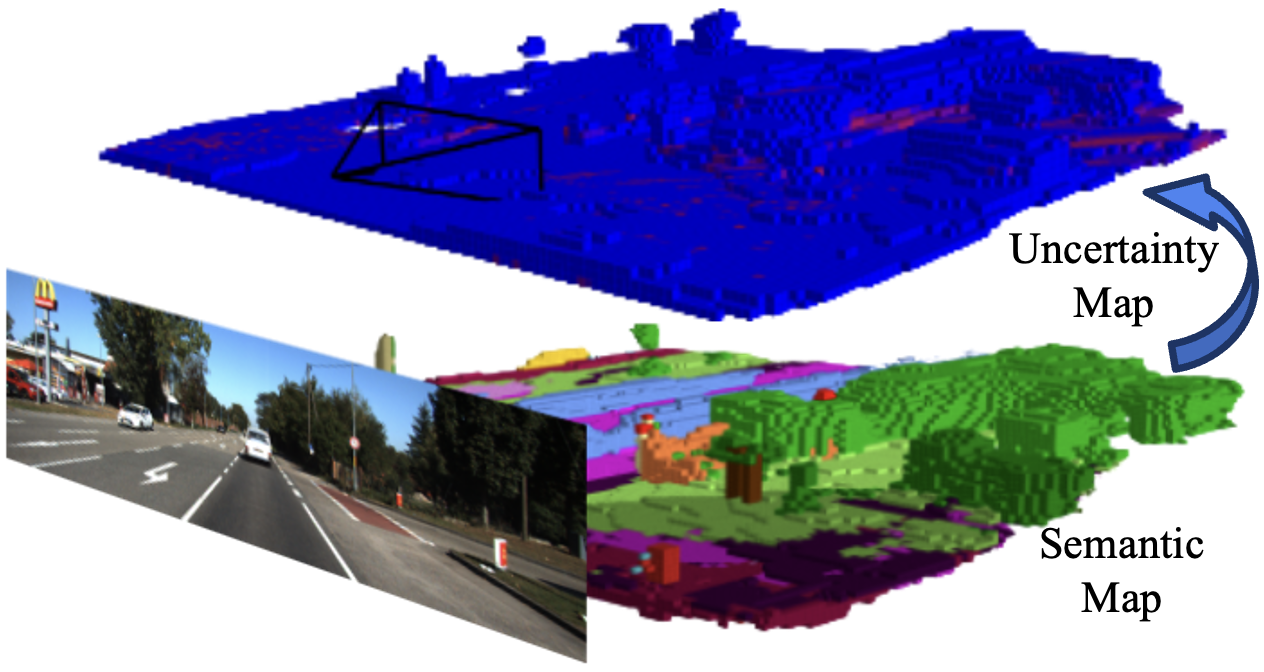
Figure 1: Our ET-Former predicts the semantic occupancy map from a monocular camera image to complete the scene and estimate the uncertainties of the occupancy map.

Main Contributions: In this work, we address the challenge of accurate semantic estimation by proposing a triplane-based deformable attention model that uses deformable attention mechanism [zhu2020deformable, xia2022vision] to process voxel and RGB features in three orthogonal views. Our approach provides a better geometric understanding from three views than only mono-cam frame and our invented deformable attention also reduces the computational cost of feature processing. To predict occluded and out-of-view regions, we employ a Conditional Variational AutoEncoder (CVAE) to generate semantic voxel predictions and also estimate the uncertainties of the predictions. Our approach takes advantage of the two stages idea from VoxFormer [li2023voxformer], where the first stage estimates occupancy from the mono-camera, providing guidance to the second stage for completing the 3D semantic occupancy map. Moreover, our triplane-based feature processing mechanism improves upon the deformable attention model in VoxFormer by smoothing estimation noise generated by sparse query voxels, and our CVAE generator performs more accurate prediction than other approaches. Our main contributions are as follows:

1. We introduce a triplane deformable model that converts 2D image features into a 3D semantic occupancy map by projecting 3D voxel queries onto three orthogonal planes, where self- / cross-deformable attentions are applied. This model significantly reduces GPU memory usage of existing methods by $25\%-50.5\%$ while refining visual and geometric information from multiple views. It achieves the highest IoU and mIoU, surpassing other methods by at least $15.16\%$ in IoU and $18.12\%$ in mIoU on the Semantic KITTI dataset.

2. We designed an efficient cross deformable attention model for multiple source feature processing, such as 2D image features with 3D voxel features. The deformable attention model reduces the computational cost by using flexible number of reference points in the deformable attention mechanism.

3. We adapt the formulation of CVAE, treating voxel queries as latent variables and reparameterizing them as Gaussian distributions to quantify uncertainty in the predicted occupancy map from stage 1, producing an uncertainty map. The integration of uncertainty and semantic maps will enable design of both safe and permissible navigation strategies in the future.

4. We apply the Triplane deformable model to stage 1 by fully leveraging image features to improve occupancy prediction accuracy.

II Related Works

Camera-based Scene Understanding: 3D scene understanding using cameras requires a comprehensive understanding of both geometric and color information [han2019image, li2022bevformer, huang2021bevdet], such as 3D scene reconstruction [popov2020corenet, li2023voxformer], 3D object detection [huang2023tri, huang2021bevdet], and 3D depth estimation [zhang2022dino, lin2017feature]. For tasks like detection and depth estimation, pixels and points are widely utilized to represent 3D objects [huang2021bevdet, huang2023tri, zhang2022dino, lin2017feature]. In scene reconstruction and completion tasks, early methods applied Truncated Signed Distance Functions (TSDFs) to process features [dai2020sg, park2019deepsdf]. Then voxel-based approaches gained more popularity due to their sparsity and memory efficiency [cao2022monoscene, li2023voxformer]. However, converting RGB features to 3D voxel features remains challenging because it requires both color and geometric understanding of the environment. To address this, Bird’s-Eye-View (BEV) scene representations are commonly used [li2022bevformer, zhang2022beverse]. The Lift-Splat-Shoot (LSS) method [philion2020lift] projects image features into 3D space using pixel-wise depth to generate BEV features. BEV-based methods like BevFormer [li2022bevformer] and PolarFormer [jiang2023polarformer] leverage attention mechanisms to learn the correlation between image features and 3D voxel features. These methods explicitly construct BEV features, while other works implicitly process BEV features within the network [reiser2021kilonerf, chen2021learning, huang2023tri], demonstrating higher computational efficiency and the ability to encode arbitrary scene resolutions. Recently, triplane features have been introduced to extend BEV representations [huang2023tri, shue20233d], projecting point features into three orthogonal planes instead of a single BEV plane. This approach has shown improved accuracy in 3D object detection [huang2023tri, huang2024gaussianformer]. However, these triplane-based approaches process do not process the voxels in the entire 3D scenarios. In our approach, we designed an efficient deformable-attention model to address the issue.

Semantic Scene Completion: Semantic Scene Completion (SSC) involves estimating both the geometry and semantic labels of a 3D scene, a task first introduced by SSCNet [li2023sscnet]. Early methods [chen20203d, zhou2022cross, song2017semantic, reading2021categorical] utilized geometric information to correlate 2D image features with 3D space. MonoScene [cao2022monoscene] and LMSCNet [roldao2020lmscnet] with monocular cameras proposed end-to-end solutions that convert RGB images into 3D semantic occupancy maps through convolutional neural networks (CNNs) or U-Net architectures. TPVFormer [huang2023tri] applied triplane features for pixel processing with multiple cameras but struggled with filling in missing areas effectively and heavy memory usages. More recent approaches like OccFormer [zhang2023occformer] and VoxFormer [li2023voxformer] have utilized transformers to enhance feature processing with monocular cameras. VoxFormer decouples occupancy and semantic predictions into two stages to improve accuracy in both semantic estimation and occlusion prediction. Building on VoxFormer, MonoOcc [zheng2024monoocc] and Symphonize [jiang2024symphonize] introduced more complex structures for both stages, further enhancing occupancy prediction and semantic estimation, though at the expense of higher memory usage. However, these methods do not estimate the certainty of semantic predictions, limiting their effectiveness in downstream tasks. To address this, we design a triplane-based deformable attention model to improve the estimation accuracy and incorporate Conditional Variational AutoEncoder (CVAE) method to predict the uncertainty of semantic estimations.

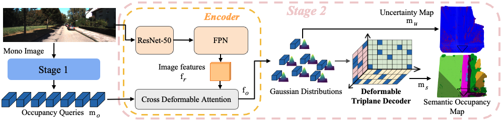
Figure 2: Architecture: We present a two-stage pipeline for processing mono-cam images and generate both a semantic occupancy map and its corresponding uncertainty map. In the second stage, we introduce an efficient triplane-based deformable attention mechanism, which reduces high-dimensional 3D feature processing to 2D computations. To estimate the uncertainty in the semantic map, we incorporate a CVAE method. In the first stage, we also apply the triplane-based deformable attention model to generate the occupancy queries, as shown in Figure 4.

III Our Approach

In this section, we introduce the problem definition, key innovations including the efficient triplane-based deformable 3D attention mechanism, and the Conditional Variational Autoencoder (CVAE) formulation.

III-A Problem Definition

We formulate the Semantic Scene Completion (SSC) task as a generative problem. Given a monocular image $\mathbf{I}\in\mathbb{R}^{H\times W\times 3}$, where $(H,W)$ represents the image size, our model aims to generate a semantic occupancy map $\mathbf{M}\in\mathbb{R}^{L\times V\times D\times N}$, where $(L,V,D)$ represents the dimensions of the 3D occupancy map and $N$ is the number of semantic classes. The model follows a CVAE formulation:

$$p(\mathbf{m}_{s}|\mathbf{c}) =\int_{\mathbf{z}}p(\mathbf{m}_{s}|\mathbf{z},\mathbf{c})p(\mathbf{z})d\mathbf{z},\;\;\;\mathbf{z}\sim p_{\theta}(\mathbf{z}|\mathbf{i}),$$ (1)

where $\mathbf{m}_{s}\in\mathbf{M}$ is the generated semantic occupancy map and $\mathbf{c}$ indicates the condition, which contains image features in our approach. The embedding vector $\mathbf{z}$ is encoded by the encoder $p_{\theta}()$, given the image instance $\mathbf{i}\in\mathbf{I}$. As illustrated in Figure 2, the model consists of a two-stage architecture for the SSC task. In the first stage, the occupancy map (queries) $\mathbf{m}_{o}\in\mathbb{R}^{L\times V\times D\times 2}$ is estimated. It serves as the inference (occupancy) for semantic prediction. In the second stage, the semantic occupancy map is generated using the CVAE formulation, with the inferred voxels from stage one as input and conditioned on the RGB image.

Our encoder in the second stage employs ResNet-50 [he2016deep] and FPN [lin2017feature], which have demonstrated high potential in image feature extraction for vision tasks [li2023voxformer, zheng2024monoocc, zhang2022dino], to process the RGB image into a lower-dimensional vector $\mathbf{f}_{r}\in\mathbb{R}^{w,h,d}$ as image features, where $w<W$, $h<H$, and $d$ denotes the feature dimension. Similar to VoxFormer [li2023voxformer], DETR [zhu2020deformable] is used to enhance the occupancy queries $\mathbf{m}_{o}$ by incorporating the image features $\mathbf{f}_{r}$ and outputs an enhanced query features $\mathbf{f}_{o}$ as follows:

$$\mathbf{f}_{o}=DETR(\mathbf{z}_{q},\mathbf{p}_{o},\mathbf{f}_{r})=$$

$$\sum_{m=1}^{M}\mathbf{W}_{m}[\sum_{k=1}^{K}A_{mqk} \mathbf{W}^{\prime}_{m}\mathbf{f}_{r}(\phi_{s}(\hat{\mathbf{p}}_{o})+\phi_{o}(\mathbf{z}_{q}))],$$ (2)

where $M$ and $K$ indicate the head number and offset number. $\mathbf{p}_{o}$ represents the 3D position of each query voxel. $\mathbf{z}_{q}=\mathbf{f}_{e}(\mathbf{p}_{o})$ is the positional embedding of the query positions. $\phi_{s}$ scales the normalized position $\hat{\mathbf{p}}_{o}$ into the image feature size $h\times w$, and $\phi_{o}$ calculates the positional offset with $\mathbf{z}_{q}$. $\mathbf{W}_{m}$ and $\mathbf{W}^{\prime}_{m}$ are linear weights. $A_{mqk}=\phi_{a}(\mathbf{z}_{q})$ is also computed from $\mathbf{z}_{q}$, where $\phi_{a}()$ represents Linear layers.

III-B Conditional Variational Autoencoder Formulation

Our approach utilizes a Conditional Variational Autoencoder (CVAE) to generate semantic occupancy maps, leveraging the unique properties of the CVAE method [bao2017cvae, harvey2021conditional, sohn2015learning]: 1. CVAEs enable conditional generation, allowing for the generation of voxels that adhere to specific conditional information. We employ this capability to generate semantic maps that conform to the RGB information from monocular observations. 2. CVAEs learn a latent space conditioned on specific attributes, which is typically smooth and continuous. This property ensures that small changes in the latent space lead to meaningful variations in the generated voxels, enhancing the expressiveness of our semantic maps. 3. CVAEs inherently model uncertainty in the generated data, accommodating cases with multiple valid outputs for the same condition, unlike deterministic models. This probabilistic nature allows our approach to handle uncertainty in monocular semantic occupancy mapping more effectively.

Given the query features $\mathbf{f}_{o}$, in the CVAE format, we need to convert the feature embedding to the embedding of Gaussian distributions, which are shown in Equation 3

$$\mu=\mathbf{l}_{m}(\mathbf{f}_{o}),\;\;\;\log\text{var}=\mathbf{l}_{v}(\mathbf{f}_{o}),$$ (3)

where $\mathbf{l}_{m}$ and $\mathbf{l}_{v}$ are linear layers. The variance of the Gaussian distribution represents the uncertainty in the estimation $\mathbf{m}_{u}$, as depicted in Figure 2.

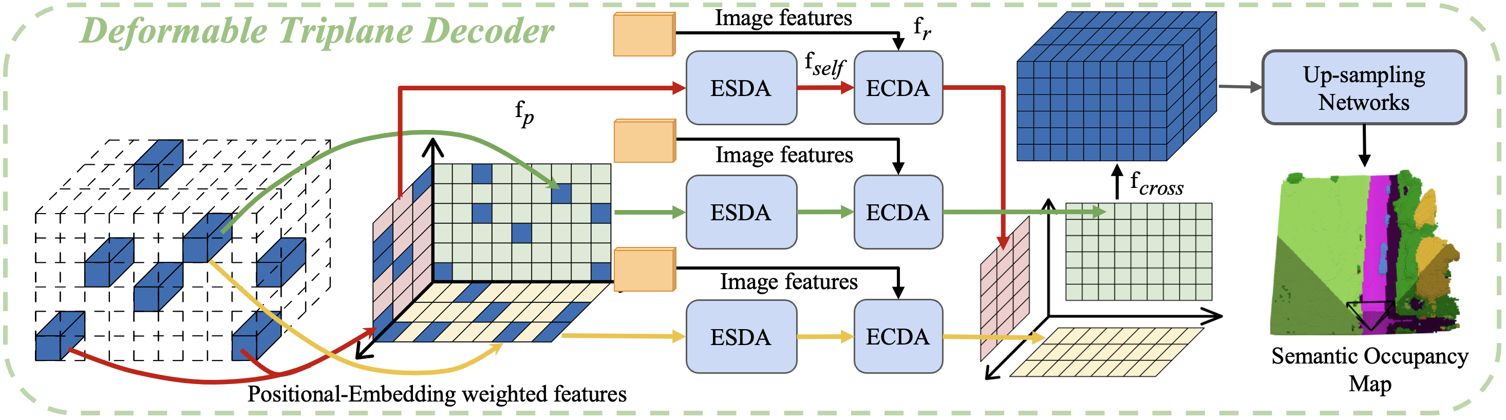
Figure 3: The Second Stage: We propose triplan-based efficient self-deformable attention (ESDA) and efficient cross-deformable attention (ECDA) methods in this stage to generate 3D features. The input for this stage consists of occupancy queries and image features. The query features are projected onto three orthogonal planes based on positional embedding weights. The three planes are filled by the ESDA method and then enhanced with image features, $\mathbf{f}_{r}$, by the ECDA method. Finally, the plane features are concatenated and upsampled to generate the semantic occupancy map.

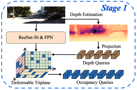
Figure 4: The First Stage: We apply the novel triplane-based deformable attention method in this stage. The estimated depth pixels are projected to the 3D space as depth queries to the triplane-based deformable model. The output of the first stage is an occupancy map, the occupied voxels in which are then converted to occupancy queries.

III-C Triplane-based 3D Deformable Attention

The triplane-based representation [huang2023tri, shue20233d] encodes 3D features by leveraging three orthogonal 2D feature planes ($XY$, $XZ$, and $YZ$). This approach significantly reduces both memory and computational requirements compared to directly encoding features in dense 3D grids. In comparison to bird’s-eye-view representations, triplane encoding offers a more sufficient representation of the real-world environment. The orthogonality of the three planes provide a robust embedding of spatial features within the 3D space, making it an effective and efficient representation for complex 3D scenes. The deformable attention mechanism [zhu2020deformable, xia2022vision] is efficient in processing high-resolution features with spatial awareness of image pixels. However, current methods [zhu2020deformable, li2023voxformer] still rely on large sets of query and reference points, resulting in high computational costs for 3D feature processing. To address this, we propose an efficient triplane-based deformable attention method that enhances voxel features with image features, improving the efficiency and performance of cross-source feature extraction.

We propose an efficient deformable triplane decoder in stage two. Instead of querying the entire 3D voxel space, we reduce the dimensionality from 3D to 2D by aggregating voxel features onto three orthogonal planes. We then propose efficient self- and cross-deformable attention mechanisms to process the features of these planes. As shown in Figure 3, the query features are aggregated by the positional embedding weights:

$$\mathbf{f}_{p}[x,y]=\sum_{z=0}^{Z}\mathbf{p}_{e}(\mathbf{p}_{o})\circ\mathbf{f}_{o},$$ (4)

where $x$ and $y$ are the pixel indices in a plane, which also correlate to the $x,y$ in the 3D space, and $z$ represents the third axis in the 3D space. The same aggregation process also applies to other two planes. The notation $\circ$ in Eqn (4) represents element-wise product.

Since queries projected from 3D space to 2D planes only occupy part of the 2D space, there are empty pixels in the 2D space. Therefore, to have a full representation of the 3D space, we must fill in the missing pixel features. We employ the Deformable Transformer [xia2022vision] to complete the missing pixel features, using plane-wide pixel features as queries and sampling reference points at a stride of four pixels. The Efficient Self-Deformable Attention (ESDA) mechanism completes the three planes, as $\mathbf{f}_{\text{self}}=\text{ESDA}(\mathbf{f}_{p})$.

As the decoder follows the CVAE format, we leverage visual features to enhance the three orthogonal planes, where the condition is the image feature $\mathbf{f}_{r}$. We introduce a new Efficient 3D Cross Deformable Attention (ECDA) model to enhance the plane features $\mathbf{f}_{\text{self}}$ with the image feature $\mathbf{f}_{r}$. Since the plane features are converted from 3D to 2D, we retain 3D geometric representation by normally sampling reference points $\mathbf{p}_{r}\in\mathbb{R}^{l,v,d}$ from the 3D voxel grid, where $l\ll L$, $v\ll V$, and $d\ll D$. These points are projected to the image feature plane $\mathbb{R}^{w\times h}$, so we have $N_{r}=l\times v\times d$ reference points $\mathbf{p}_{i}\in\mathbb{R}^{l\times v\times d\times 2}$ in the image feature plane. The filled-in triplane features, $\mathbf{f}_{\text{self}}$, serve as queries in ECDA. Because the reference points are normally sampled from the 3D space, the $x,y$ coordinates are correlated to the triplane $x,y$ positions. We can use convolutional layers directly to calculate the offsets of the reference points, as $\Delta\mathbf{f}_{r}=\text{Conv}(\mathbf{f}_{\text{self}})$, where $\Delta\mathbf{f}_{r}\in\mathbb{R}^{l,v,c}$ and $c$ is the feature dimension. We separate the feature dimension into $d$ vectors to represent the offset of $d$ points in the $z$ axis. Finally, we have $\Delta\mathbf{p}_{i}=\mathbf{l}_{r}(\text{rearrange}(\Delta\mathbf{f}_{r}))$. Then a multi-head attention model is used to process the sampled image features with the plane features as in Equation 5

$$\mathbf{f}_{\text{cross}}=\text{MultiHead}(\mathbf{f}_{\text{self}},\mathbf{f}_{r}[\mathbf{p}_{i}+\Delta\mathbf{p}_{i}]),$$ (5)

where $\mathbf{f}_{\text{self}}$ is the query and $\mathbf{f}_{r}[\mathbf{p}_{i}+\Delta\mathbf{p}_{i}]$ serves as key and value of the multi-head attention model. The $\mathbf{f}_{\text{cross}}$ from three planes would be concatenated together and processed by several linear layers and upsampled to the semantic map, $\mathbf{m}_{s}=\mathbf{l}_{s}(\text{UpSample}(\mathbf{l}_{c}([\mathbf{f}_{\text{cross}}^{l},\mathbf{f}_{\text{cross}}^{h},\mathbf{f}_{\text{cross}}^{d}])))$, where $\mathbf{l}_{s}$ and $\mathbf{l}_{c}$ are all linear layers. $\mathbf{f}_{\text{cross}}^{l}$, $\mathbf{f}_{\text{cross}}^{h}$ and $\mathbf{f}_{\text{cross}}^{d}$ are features of the 2D planes orthogonal to the $l,h,d$ axes.

Methods	IoU	mIoU	road	sidewalk	parking	other-ground	building	car	truck	bicycle	motorcycle	other-vehicle	vegetation	trunk	terrain	person	bicyclist	motorcyclist	fence	pole	traffic-sign
MonoScene [cao2022monoscene]	34.16	11.08	54.70	27.10	24.80	5.70	14.40	18.80	3.30	0.50	0.70	4.40	14.90	2.40	19.50	1.00	1.40	0.40	11.10	3.30	2.10
TPVFormer [huang2023tri]	34.25	11.26	55.10	27.20	27.40	6.50	14.80	19.20	3.70	1.00	0.50	2.30	13.90	2.60	20.40	1.10	2.40	0.30	11.00	2.90	1.50
VoxFormer [li2023voxformer]	42.95	12.20	53.90	25.30	21.10	5.60	19.80	20.80	3.50	1.00	0.70	3.70	22.40	7.50	21.30	1.40	2.60	0.20	11.10	5.10	4.90
OccFormer [zhang2023occformer]	34.53	12.32	55.90	30.30	31.50	6.50	15.70	21.60	1.20	1.50	1.70	3.20	16.80	3.90	21.30	2.20	1.10	0.20	11.90	3.80	3.70
MonoOcc [zheng2024monoocc]	-	13.80	55.20	27.80	25.10	9.70	21.40	23.20	5.20	2.20	1.50	5.40	24.00	8.70	23.00	1.70	2.00	0.20	13.40	5.80	6.40
Symphonize [jiang2024symphonize]	41.44	13.44	55.78	26.77	14.57	0.19	18.76	27.23	15.99	1.44	2.28	9.52	24.50	4.32	28.49	3.19	8.09	0.00	6.18	8.99	5.39
OctreeOcc [lu2023octreeocc]	44.71	13.12	55.13	26.74	18.68	0.65	18.69	28.07	16.43	0.64	0.71	6.03	25.26	4.89	32.47	2.25	2.57	0.00	4.01	3.72	2.36
ET-Former (Ours)	51.49	16.30	57.64	25.80	16.68	0.87	26.74	36.16	12.95	0.69	0.32	8.41	33.95	11.58	37.01	1.33	2.58	0.32	9.52	19.60	6.90

TABLE I: Semantic Scene Completion: Our ET-Former outperforms other approaches, showing at least $15.16\%$ and $18.12\%$ improvements in IoU and mIoU. For specific semantic categories, such as road, building, car, vegetation, trunk, terrain, pole, and traffic-sign, our model provides the best accuracy.

RGB	Ground Truth	ET-Former	VoxFormer [li2023voxformer]	MonoScene [cao2022monoscene]

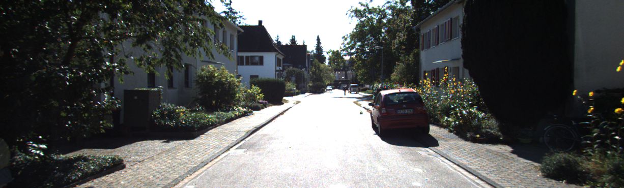
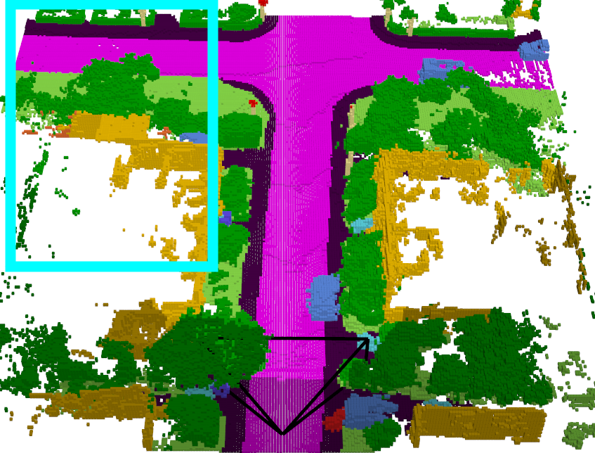
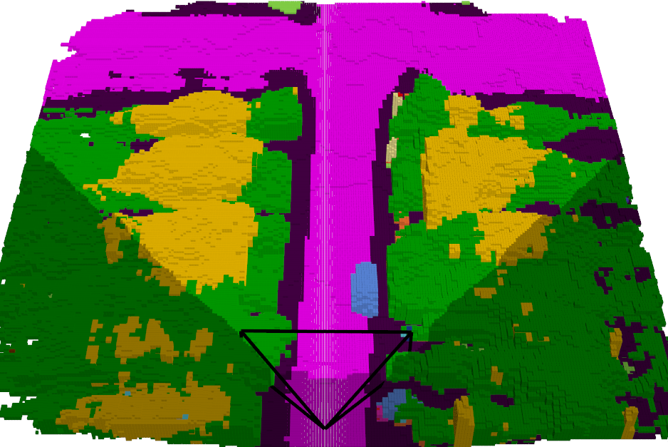
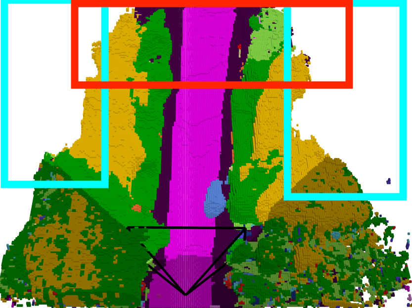
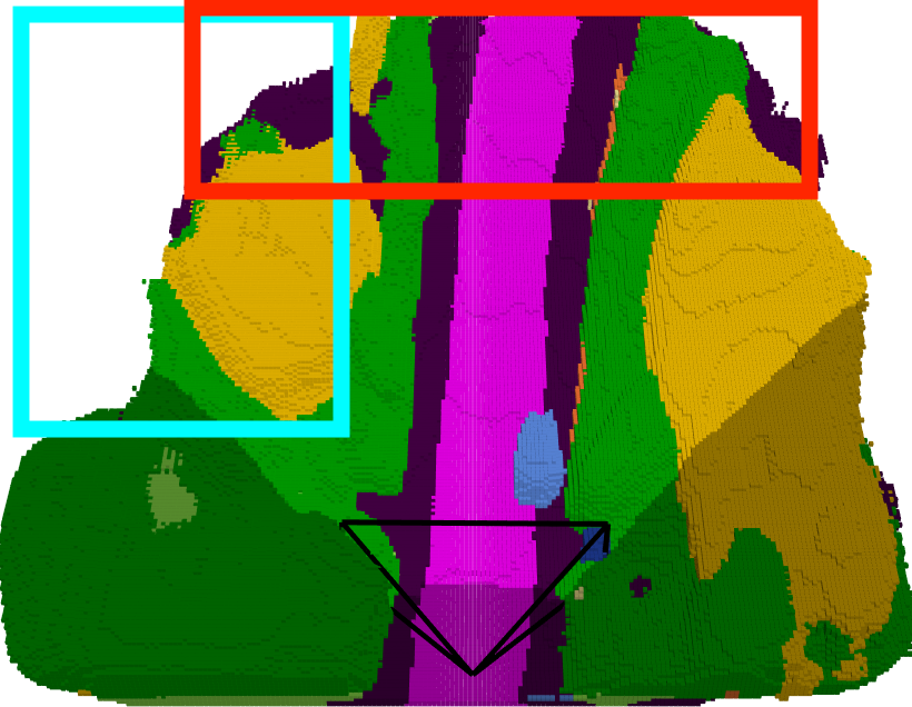
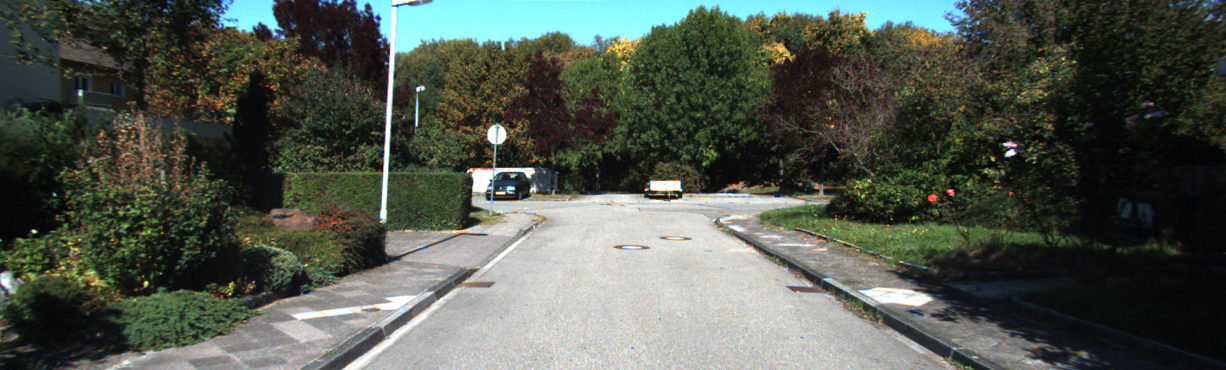
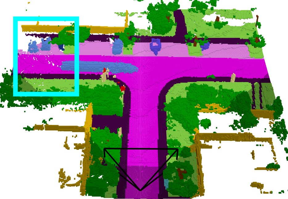
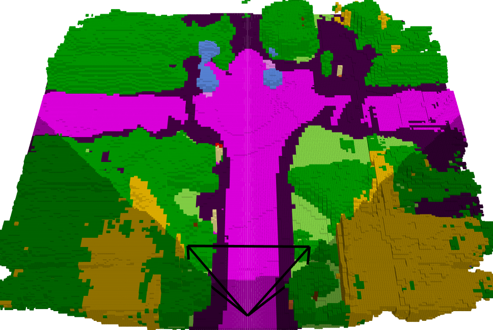
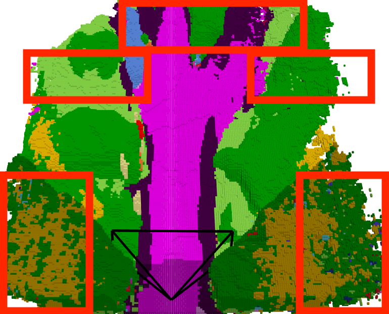
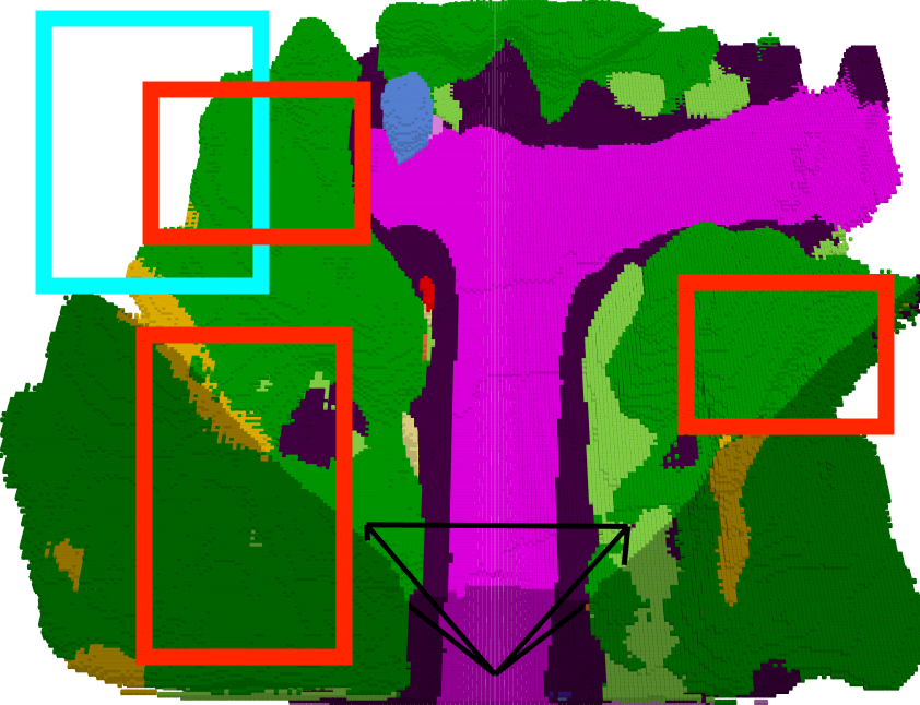
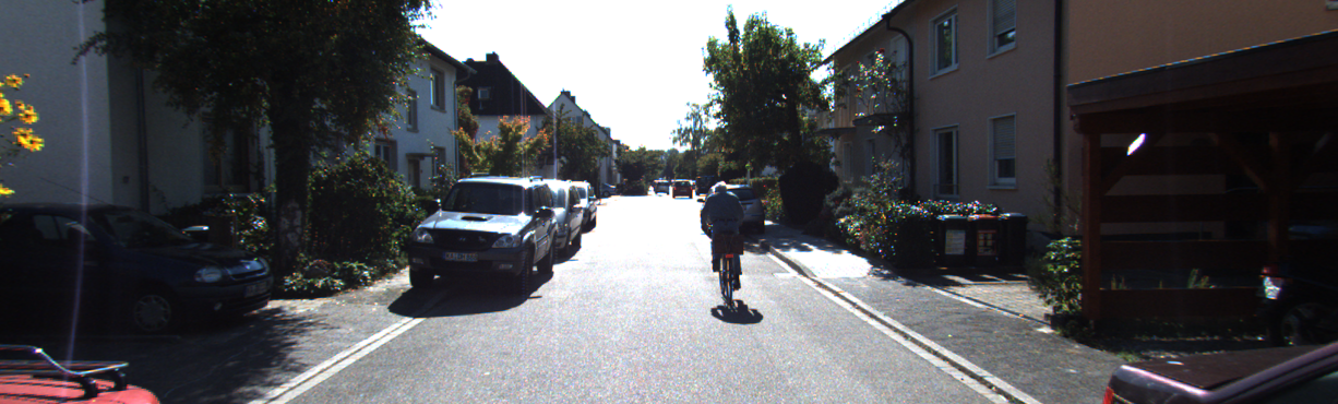
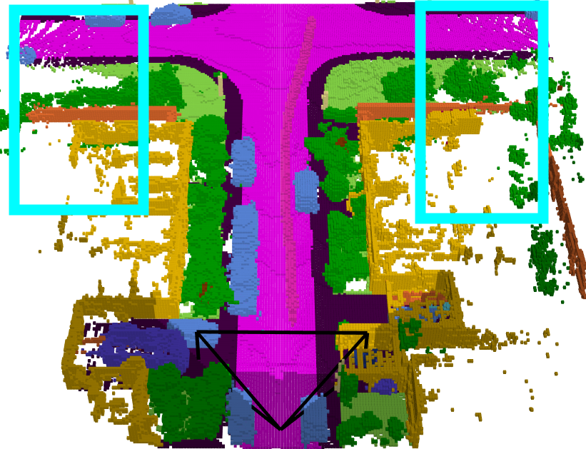
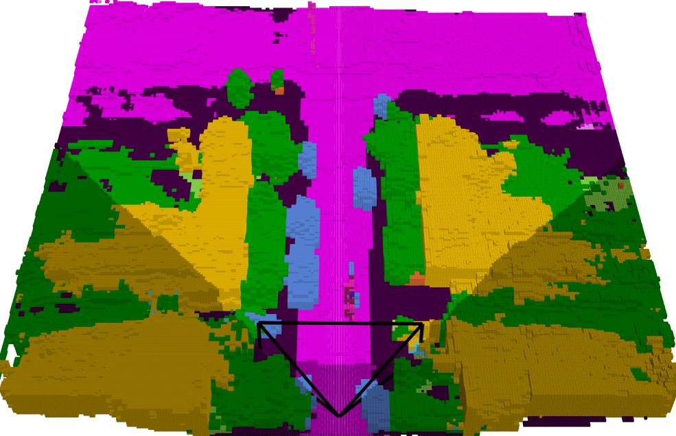
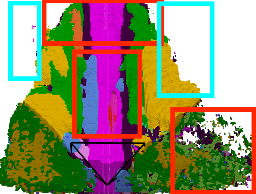
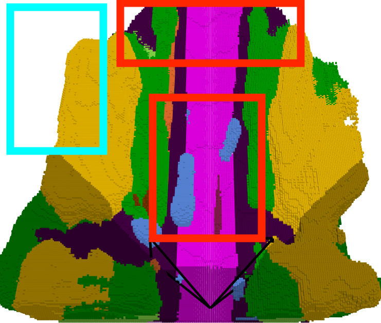
Figure 5: Semantic Qualitative Results: The blue rectangles indicate missing areas where VoxFormer and MonoScene do not have but Ground Truth contains. The red rectangles marked the areas with wrong semantic estimations.

RGB	Ground Truth	ET-Former	Uncertainty

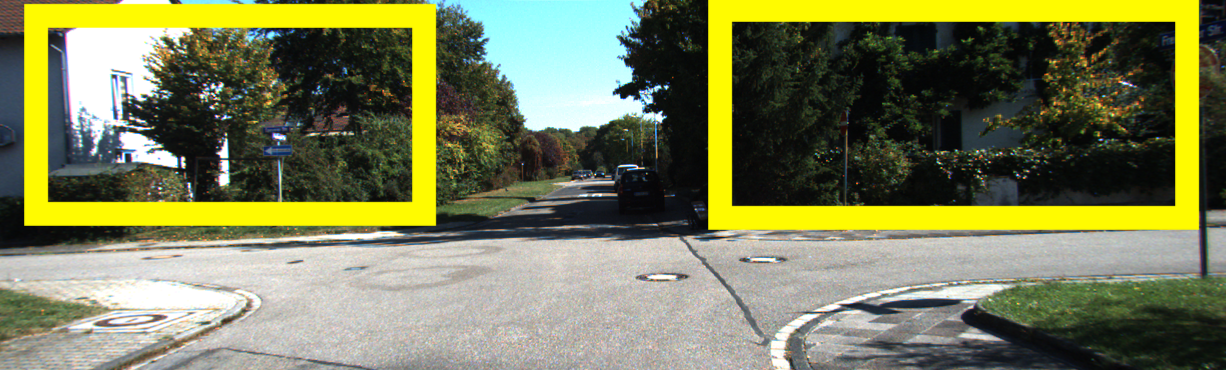
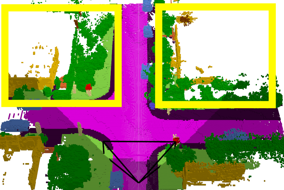
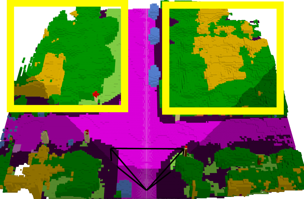
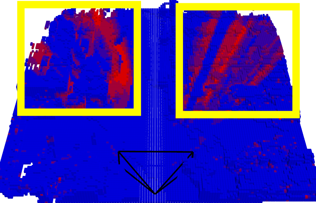
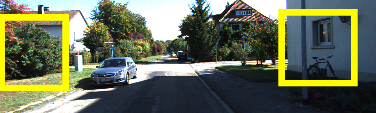
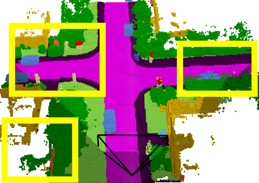
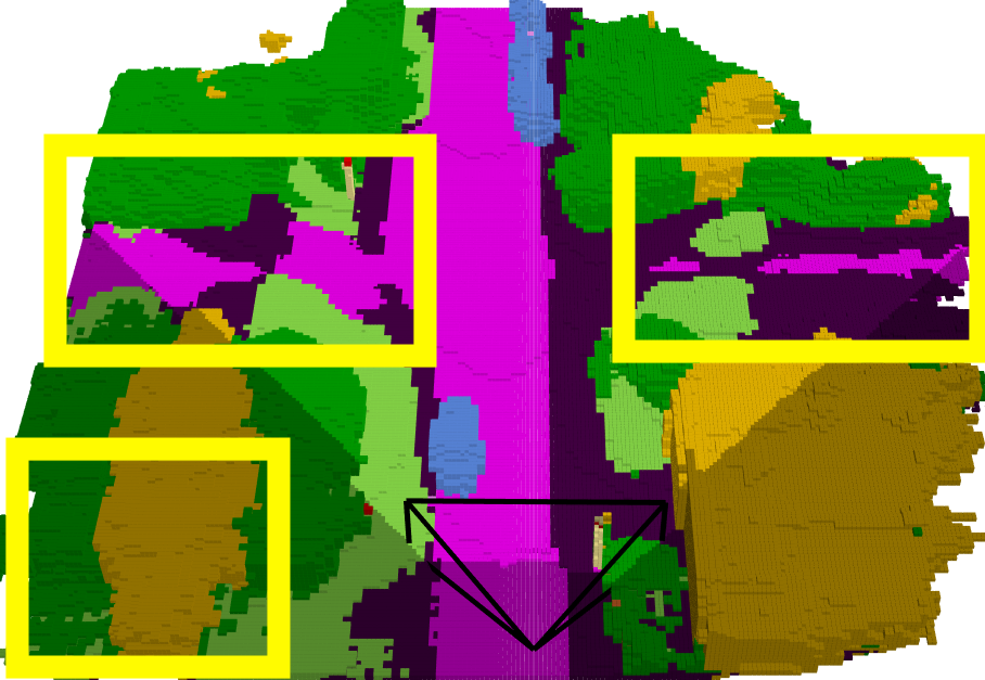
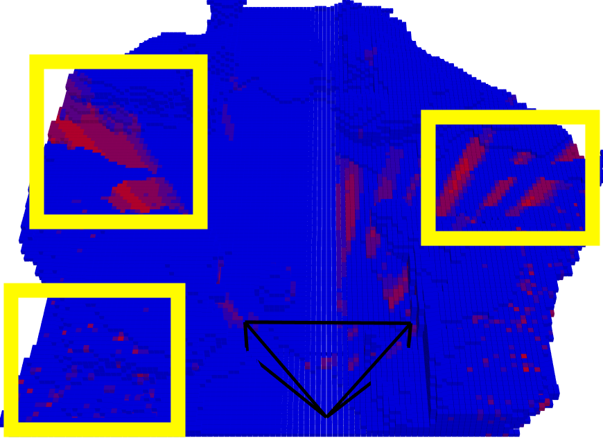
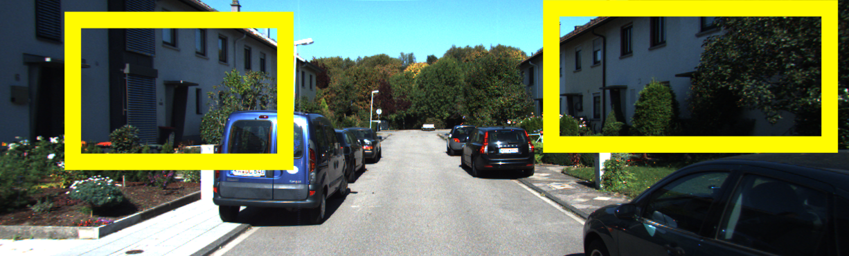
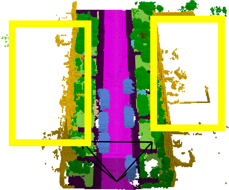
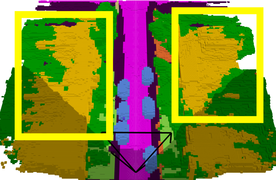
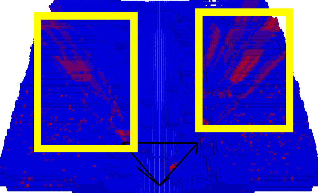
Figure 6: Uncertainty Qualitative Results: In column 3, blue voxels show low uncertainty areas, while red voxels, highlighted by yellow rectangles, indicate high uncertainty. These uncertain areas are typically outside the camera’s FOV, or obscured by vegetation (row 1) or buildings (rows 2-3).

III-D Occupancy Prediction

In the first stage, the occupancy map $\mathbf{m}_{o}$ is estimated, which identifies occupied voxels in 3D space. As shown in Figure 4, we estimate depth from the RGB image, and then the depth pixels are projected into 3D space and voxelized into an occupancy map. The initial map is often inaccurate due to raw depth estimation. Following a similar approach to stage two, we use ResNet-50 and FPN to process image features, enhancing the occupancy map with the triplane-based deformable attention model described in Section III-C. In the triplane model, we use positional embeddings as the query features and aggregate them into three orthogonal planes. The output of the triplane model is an occupancy map $\mathbf{m}_{o}=\mathbf{l}_{o}([\mathbf{f}_{\text{cross}}^{l},\mathbf{f}_{\text{cross}}^{h},\mathbf{f}_{\text{cross}}^{d}])$, where $\mathbf{l}_{o}$ is a linear layer.

III-E Training Strategy

The two stages are trained separately, using a cosine scheduler. Given that the ground truth occupancy map $\mathbf{m}_{o}^{gt}$ is derived from a sequence of LIDAR data, which may include occlusions, we mask out missing and unlabeled voxels during training. Stage one uses a cross-entropy loss $\mathcal{L}_{ce}(\mathbf{m}_{o}^{gt},\mathbf{m}_{o})$ for occupancy prediction.

The second stage is trained in the formulation of CVAE, so we have the CVAE lower bound loss function:

$$\mathcal{L}_{C}=-\mathcal{D}_{KL}(p_{\theta}(\mathbf{z}|\mathbf{m}_{o},\mathbf{f}_{r})\parallel p(\mathbf{z}))+\sum\log p(\mathbf{m}_{s}|\mathbf{f}_{r},\mathbf{z}),$$

where $p()$ represents the probability. Besides $\mathcal{L}_{C}$, reconstruction losses including class-weighted cross-entropy loss $\mathcal{L}_{ce}$, and losses $\mathcal{L}_{scal}^{sem}$ and $\mathcal{L}_{scal}^{geo}$ from [cao2022monoscene] are used.

IV Experiments

Dataset and Evaluation Metrics: In this work, various experiments were conducted to evaluate the proposed 3D uncertainty semantic prediction framework using the SemanticKITTI [behley2019semantickitti] dataset with monocular cameras. SemanticKITTI provides the semantic ground truth data in the range of $[0\ \text{m},51.2\ \text{m}]\times[-25.6\ \text{m},25.6\ \text{m}]\times[-2\ \text{m},4.4\ \text{m}]$. The semantic occupancy map has the shape of $256\times 256\times 32$ voxels, while the occupancy map for stage one has the shape $128\times 128\times 16$. Each voxel in the semantic occupancy map has 20 classes of semantic labels consisting of 19 semantic classes and 1 free class. Following the regular metric for SSC tasks, we utilize the Intersection over Union (IoU) to evaluate the occupancy prediction and the scene completion quality in stages one and two. For semantic evaluation, we use the mean IoU (mIoU) of the 19 semantic classes to evaluate the performance of the semantic prediction. Furthermore, we enumerate all 19 classes to evaluate the accuracy of the methods in each semantic class estimation. The training and evaluation are done by one GPU V100.

IV-A Comparisons

Table I compares our approach, ET-Former, with state-of-the-art methods. Our model achieves the highest IoU and mIoU, surpassing other methods by at least $15.16\%$ in IoU and $18.12\%$ in mIoU. The triplane-based feature representation proves particularly effective for commonly seen, large semantic objects. We achieve the best semantic accuracy across multiple categories, such as road, building, car, vegetation, trunk, terrain, pole, and traffic-sign.

We evaluated the memory usage of ET-Former against VoxFormer [li2023voxformer] and others in training memory consumption (Table II). ET-Former reduces GPU memory usage by 3.7 GB $(25\%)$ compared to VoxFormer, and by 11.1 GB $(50.5\%)$ compared to Symphonize [jiang2024symphonize], while significantly outperforming them in IoU and mIoU. These results highlight the efficiency of the proposed method.

Methods	IoU	mIoU	Memory
VoxFormer [li2023voxformer]	42.95	12.20	14.6 Gb
MonoScene [cao2022monoscene]	34.16	11.08	18.9 Gb
Symphonize  [jiang2024symphonize]	41.44	13.44	22.0 Gb
TPVFormer [huang2023tri]	34.25	11.26	23.0 Gb
ET-Former	51.49	16.30	10.9 Gb

TABLE II: Memory Usage: Our method reduces GPU memory usage by 3.7 GB $(25\%)$ compared to VoxFormer [li2023voxformer], and by 11.1 GB $(50.5\%)$ compared to Symphonize [jiang2024symphonize], while outperforming them in IoU and mIoU.

For the evaluation of our first-stage occupancy prediction, we compared our results with those of VoxFormer, as presented in Table IV in Section VI. Our model achieves $14\%$ and $16.3\%$ improvements in IoU and Recall, respectively.

IV-B Ablation Study

Table III presents an ablation analysis of the architectural components, using VoxFormer [li2023voxformer] as the baseline. Replacing VoxFormer’s second stage with our deterministic second stage model (where query features $\mathbf{f}_{o}$ are directly fed into the deformable triplane decoder instead of converting to Gaussian distributions as in (3)) improves IoU by 0.36 and mIoU by 0.28 compared to the baseline. Implementing our CVAE stochastic second stage further enhances performance by 0.63 IoU and 0.57 mIoU. Finally, combining our first stage model with the CVAE stochastic second stage significantly boosts performance by 7.57 IoU and 3.25 mIoU.

Methods	IoU	mIoU
Baseline (VoxFormer [li2023voxformer])	42.95	12.20
+ Our deterministic stage 2	43.29 (+0.36)	12.48 (+0.28)
+ Our stochastic stage 2	43.92 (+0.63)	13.05 (+0.57)
+ Our stage 1 + stochastic stage 2	51.49 (+7.57)	16.30 (+3.25)

TABLE III: Ablation Study: our key components (deformable triplane decoder, CVAE formulation, and proposed first stage model) each contribute to significant improvements in semantic estimation accuracy.

IV-C Visualizations

Qualitative Results: Figure 5 qualitatively compares our approach with VoxFormer [li2023voxformer] and MonoScene [cao2022monoscene]. Blue rectangles highlight areas missed by other methods, while red rectangles indicate incorrect semantic estimations. VoxFormer shows considerable noise in its predictions, especially outside the camera’s FOV, and struggles with occluded areas (e.g., the driving road in the third row). MonoScene has difficulty estimating semantics in occluded areas and completing the map. In contrast, our ET-Former effectively handles occluded and out-of-FOV areas.

Uncertainty Map visualization: In Figure 6, we evaluate the uncertainties in the estimated semantic occupancy map. The yellow rectangles highlight areas with high uncertainty, which mainly arise from occlusions and regions outside the camera’s FOV. For example, in the first and third rows, areas behind vegetation and buildings exhibit significant uncertainties, respectively, with the uncertainty extending outward from these objects along the camera’s line of sight. In the second row, while the horizontal road is blocked by inaccurately estimated terrain, our method assigns high uncertainty values to these problematic areas. This uncertainty quantification helps identify regions where the occupancy estimation may be less reliable, potentially aiding in formulation of risk-aware navigation strategies.

V Conclusion, Limitations, and Future Work

ET-Former offers an efficient and robust solution for 3D semantic scene completion using a single monocular camera. It successfully achieves state of the art performance with much less memory usage, highlighting its potential for real-world applications in autonomous navigation systems. Our future work could focus on designing a more memory-efficient yet effective encoder. Additionally, we aim to design a navigation strategy that makes safe but also permissible decisions leveraging both semantic and uncertainty maps generated from the proposed algorithm.

VI Appendix

VI-A Results of the First Stage

For the first stage model proposed in Section III-D, to ensure a fair comparison, we utilize the same depth estimation method, MobileStereoNet [shamsafar2022mobilestereonet], as employed by the stage one of VoxFormer. Following this, as depicted in Figure 4, we apply our triplane-based method to generate the occupancy map and queries. The quality of the occupancy map predictions is compared between our stage one approach and VoxFormer’s, as shown in Table IV. Our approach shows substantial improvements, with a $14\%$ increase in IoU and a $16.3\%$ increase in Recall, resulting in a more accurate occupancy map and more efficient occupancy queries. These enhancements ultimately improve the performance of the subsequent semantic predictions, as shown in Table III.

Methods	IoU	Recall
VoxFormer’s stage one	52.03	61.52
Our stage one	59.41	71.56

TABLE IV: Results of the First Stage: Compared with the VoxFormer’s stage one model, our stage one model achieves $14\%$ and $16.3\%$ improvements in IoU and Recall values, respectively.

References

- [1] A. Saxena, M. Sun, and A. Y. Ng, “Make3d: Learning 3d scene structure from a single still image,” IEEE transactions on pattern analysis and machine intelligence, vol. 31, no. 5, pp. 824–840, 2008.
- [2] C. Zhang, Z. Cui, Y. Zhang, B. Zeng, M. Pollefeys, and S. Liu, “Holistic 3d scene understanding from a single image with implicit representation,” in Proceedings of the IEEE/CVF Conference on Computer Vision and Pattern Recognition, 2021, pp. 8833–8842.
- [3] Y. Li, Z. Yu, C. Choy, C. Xiao, J. M. Alvarez, S. Fidler, C. Feng, and A. Anandkumar, “Voxformer: Sparse voxel transformer for camera-based 3d semantic scene completion,” in Proceedings of the IEEE/CVF conference on computer vision and pattern recognition, 2023, pp. 9087–9098.
- [4] Y. Zheng, X. Li, P. Li, Y. Zheng, B. Jin, C. Zhong, X. Long, H. Zhao, and Q. Zhang, “Monoocc: Digging into monocular semantic occupancy prediction,” arXiv preprint arXiv:2403.08766, 2024.
- [5] A.-Q. Cao and R. De Charette, “Monoscene: Monocular 3d semantic scene completion,” in Proceedings of the IEEE/CVF Conference on Computer Vision and Pattern Recognition, 2022, pp. 3991–4001.
- [6] J. Choe, S. Im, F. Rameau, M. Kang, and I. S. Kweon, “Volumefusion: Deep depth fusion for 3d scene reconstruction,” in Proceedings of the IEEE/CVF International Conference on Computer Vision, 2021, pp. 16 086–16 095.
- [7] A. Dai, C. Diller, and M. Nießner, “Sg-nn: Sparse generative neural networks for self-supervised scene completion of rgb-d scans,” in Proceedings of the IEEE/CVF Conference on Computer Vision and Pattern Recognition, 2020, pp. 849–858.
- [8] P. Li, R. Zhao, Y. Shi, H. Zhao, J. Yuan, G. Zhou, and Y.-Q. Zhang, “Lode: Locally conditioned eikonal implicit scene completion from sparse lidar,” in 2023 IEEE International Conference on Robotics and Automation (ICRA). IEEE, 2023, pp. 8269–8276.
- [9] Z. Xia, Y. Liu, X. Li, X. Zhu, Y. Ma, Y. Li, Y. Hou, and Y. Qiao, “Scpnet: Semantic scene completion on point cloud,” in Proceedings of the IEEE/CVF conference on computer vision and pattern recognition, 2023, pp. 17 642–17 651.
- [10] A. J. Davison, I. D. Reid, N. D. Molton, and O. Stasse, “Monoslam: Real-time single camera slam,” IEEE transactions on pattern analysis and machine intelligence, vol. 29, no. 6, pp. 1052–1067, 2007.
- [11] M. Li, S. Liu, and H. Zhou, “Sgs-slam: Semantic gaussian splatting for neural dense slam,” arXiv preprint arXiv:2402.03246, 2024.
- [12] L. Roldao, R. De Charette, and A. Verroust-Blondet, “3d semantic scene completion: A survey,” International Journal of Computer Vision, vol. 130, no. 8, pp. 1978–2005, 2022.
- [13] Y. Huang, W. Zheng, Y. Zhang, J. Zhou, and J. Lu, “Tri-perspective view for vision-based 3d semantic occupancy prediction,” in Proceedings of the IEEE/CVF conference on computer vision and pattern recognition, 2023, pp. 9223–9232.
- [14] X. Zhu, W. Su, L. Lu, B. Li, X. Wang, and J. Dai, “Deformable detr: Deformable transformers for end-to-end object detection,” arXiv preprint arXiv:2010.04159, 2020.
- [15] Z. Xia, X. Pan, S. Song, L. E. Li, and G. Huang, “Vision transformer with deformable attention,” in Proceedings of the IEEE/CVF conference on computer vision and pattern recognition, 2022, pp. 4794–4803.
- [16] X.-F. Han, H. Laga, and M. Bennamoun, “Image-based 3d object reconstruction: State-of-the-art and trends in the deep learning era,” IEEE transactions on pattern analysis and machine intelligence, vol. 43, no. 5, pp. 1578–1604, 2019.
- [17] Z. Li, W. Wang, H. Li, E. Xie, C. Sima, T. Lu, Y. Qiao, and J. Dai, “Bevformer: Learning bird’s-eye-view representation from multi-camera images via spatiotemporal transformers,” in European conference on computer vision. Springer, 2022, pp. 1–18.
- [18] J. Huang, G. Huang, Z. Zhu, Y. Ye, and D. Du, “Bevdet: High-performance multi-camera 3d object detection in bird-eye-view,” arXiv preprint arXiv:2112.11790, 2021.
- [19] S. Popov, P. Bauszat, and V. Ferrari, “Corenet: Coherent 3d scene reconstruction from a single rgb image,” in Computer Vision–ECCV 2020: 16th European Conference, Glasgow, UK, August 23–28, 2020, Proceedings, Part II 16. Springer, 2020, pp. 366–383.
- [20] H. Zhang, F. Li, S. Liu, L. Zhang, H. Su, J. Zhu, L. M. Ni, and H.-Y. Shum, “Dino: Detr with improved denoising anchor boxes for end-to-end object detection,” arXiv preprint arXiv:2203.03605, 2022.
- [21] T.-Y. Lin, P. Dollár, R. Girshick, K. He, B. Hariharan, and S. Belongie, “Feature pyramid networks for object detection,” in Proceedings of the IEEE conference on computer vision and pattern recognition, 2017, pp. 2117–2125.
- [22] J. J. Park, P. Florence, J. Straub, R. Newcombe, and S. Lovegrove, “Deepsdf: Learning continuous signed distance functions for shape representation,” in Proceedings of the IEEE/CVF conference on computer vision and pattern recognition, 2019, pp. 165–174.
- [23] Y. Zhang, Z. Zhu, W. Zheng, J. Huang, G. Huang, J. Zhou, and J. Lu, “Beverse: Unified perception and prediction in birds-eye-view for vision-centric autonomous driving,” arXiv preprint arXiv:2205.09743, 2022.
- [24] J. Philion and S. Fidler, “Lift, splat, shoot: Encoding images from arbitrary camera rigs by implicitly unprojecting to 3d,” in Computer Vision–ECCV 2020: 16th European Conference, Glasgow, UK, August 23–28, 2020, Proceedings, Part XIV 16. Springer, 2020, pp. 194–210.
- [25] Y. Jiang, L. Zhang, Z. Miao, X. Zhu, J. Gao, W. Hu, and Y.-G. Jiang, “Polarformer: Multi-camera 3d object detection with polar transformer,” in Proceedings of the AAAI conference on Artificial Intelligence, vol. 37, no. 1, 2023, pp. 1042–1050.
- [26] C. Reiser, S. Peng, Y. Liao, and A. Geiger, “Kilonerf: Speeding up neural radiance fields with thousands of tiny mlps,” in Proceedings of the IEEE/CVF international conference on computer vision, 2021, pp. 14 335–14 345.
- [27] Y. Chen, S. Liu, and X. Wang, “Learning continuous image representation with local implicit image function,” in Proceedings of the IEEE/CVF conference on computer vision and pattern recognition, 2021, pp. 8628–8638.
- [28] J. R. Shue, E. R. Chan, R. Po, Z. Ankner, J. Wu, and G. Wetzstein, “3d neural field generation using triplane diffusion,” in Proceedings of the IEEE/CVF Conference on Computer Vision and Pattern Recognition, 2023, pp. 20 875–20 886.
- [29] Y. Huang, W. Zheng, Y. Zhang, J. Zhou, and J. Lu, “Gaussianformer: Scene as gaussians for vision-based 3d semantic occupancy prediction,” arXiv preprint arXiv:2405.17429, 2024.
- [30] X. Li, F. Xu, X. Yong, D. Chen, R. Xia, B. Ye, H. Gao, Z. Chen, and X. Lyu, “Sscnet: A spectrum-space collaborative network for semantic segmentation of remote sensing images,” Remote Sensing, vol. 15, no. 23, p. 5610, 2023.
- [31] X. Chen, K.-Y. Lin, C. Qian, G. Zeng, and H. Li, “3d sketch-aware semantic scene completion via semi-supervised structure prior,” in Proceedings of the IEEE/CVF Conference on Computer Vision and Pattern Recognition, 2020, pp. 4193–4202.
- [32] B. Zhou and P. Krähenbühl, “Cross-view transformers for real-time map-view semantic segmentation,” in Proceedings of the IEEE/CVF conference on computer vision and pattern recognition, 2022, pp. 13 760–13 769.
- [33] S. Song, F. Yu, A. Zeng, A. X. Chang, M. Savva, and T. Funkhouser, “Semantic scene completion from a single depth image,” in Proceedings of the IEEE conference on computer vision and pattern recognition, 2017, pp. 1746–1754.
- [34] C. Reading, A. Harakeh, J. Chae, and S. L. Waslander, “Categorical depth distribution network for monocular 3d object detection,” in Proceedings of the IEEE/CVF Conference on Computer Vision and Pattern Recognition, 2021, pp. 8555–8564.
- [35] L. Roldao, R. de Charette, and A. Verroust-Blondet, “Lmscnet: Lightweight multiscale 3d semantic completion,” in 2020 International Conference on 3D Vision (3DV). IEEE, 2020, pp. 111–119.
- [36] Y. Zhang, Z. Zhu, and D. Du, “Occformer: Dual-path transformer for vision-based 3d semantic occupancy prediction,” in Proceedings of the IEEE/CVF International Conference on Computer Vision, 2023, pp. 9433–9443.
- [37] H. Jiang, T. Cheng, N. Gao, H. Zhang, T. Lin, W. Liu, and X. Wang, “Symphonize 3d semantic scene completion with contextual instance queries,” in Proceedings of the IEEE/CVF Conference on Computer Vision and Pattern Recognition, 2024, pp. 20 258–20 267.
- [38] K. He, X. Zhang, S. Ren, and J. Sun, “Deep residual learning for image recognition,” in Proceedings of the IEEE conference on computer vision and pattern recognition, 2016, pp. 770–778.
- [39] J. Bao, D. Chen, F. Wen, H. Li, and G. Hua, “Cvae-gan: fine-grained image generation through asymmetric training,” in Proceedings of the IEEE international conference on computer vision, 2017, pp. 2745–2754.
- [40] W. Harvey, S. Naderiparizi, and F. Wood, “Conditional image generation by conditioning variational auto-encoders,” arXiv preprint arXiv:2102.12037, 2021.
- [41] K. Sohn, H. Lee, and X. Yan, “Learning structured output representation using deep conditional generative models,” Advances in neural information processing systems, vol. 28, 2015.
- [42] Y. Lu, X. Zhu, T. Wang, and Y. Ma, “Octreeocc: Efficient and multi-granularity occupancy prediction using octree queries,” arXiv preprint arXiv:2312.03774, 2023.
- [43] J. Behley, M. Garbade, A. Milioto, J. Quenzel, S. Behnke, C. Stachniss, and J. Gall, “Semantickitti: A dataset for semantic scene understanding of lidar sequences,” in Proceedings of the IEEE/CVF international conference on computer vision, 2019, pp. 9297–9307.
- [44] F. Shamsafar, S. Woerz, R. Rahim, and A. Zell, “Mobilestereonet: Towards lightweight deep networks for stereo matching,” in Proceedings of the ieee/cvf winter conference on applications of computer vision, 2022, pp. 2417–2426.