6G RIS-aided Single-LEO Localization with Slow and Fast Doppler Effects

Abstract

6G networks aim to enable applications like autonomous driving by providing complementary localization services through key technologies such as non-terrestrial networks (NTNs) with low Earth orbit (LEO) satellites and reconfigurable intelligent surfaces (RIS). Prior research in 6G localization using single LEO, multi-LEO, and multi-LEO multi-RIS setups has limitations: single LEO lacks the required accuracy, while multi-LEO/RIS setups demand many visible satellites and RISs, which is not always feasible in practice. This paper explores the novel problem of localization with a single LEO satellite and a single RIS, bridging these research areas. We present a comprehensive signal model accounting for user carrier frequency offset (CFO), clock bias, and fast and slow Doppler effects. Additionally, we derive a low-complexity estimator that achieves theoretical bounds at high signal-to-noise ratios (SNR). Our results demonstrate the feasibility and accuracy of RIS-aided single-LEO localization in 6G networks and highlight potential research directions.

I Introduction

NTN utilize space- and airborne platforms and are expected to play a crucial role in social sustainability, enhancing network resilience, and providing continuous connectivity in scenarios where terrestrial infrastructure may be inadequate or non-existent [1]. In particular, the use of low earth orbit (LEO) satellites has the potential to provide global 6G integrated communication and sensing (e.g., positioning, imaging) services [2], complementing existing terrestrial communication systems and space-based positioning systems (e.g., GPS) [3].

Focusing on the important application of user localization, LEO-based non-terrestrial network (NTN) has been studied in various contexts, benefiting from the high satellite mobility, high-power signals, and low latencies [4, 5]. Existing studies can be divided into multi-LEO localization [6, 7, 8, 9] or single-LEO localization [4, 5, 10].

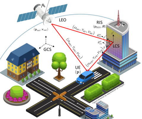
Figure 1: A 6G localization scenario with a single-LEO satellite aided by a single-RIS in an urban setting.

In the former category, [6] studied a multi-LEO system with 3GPP numerology, while [7] focused on joint localization and time-frequency synchronization in NTN-IoT applications. Opportunistic multi-LEO localization using NTN was proposed in [8], while [9] demonstrated the practical feasibility of positioning without detailed knowledge of the transmitted signal. In the latter category, [5] considered joint localization and communication from a single LEO satellite of a time-synchronized user, relying on angle-of-departure (AoD) and time-of-arrival (ToA) measurements. Note here that small AoD measurement errors will lead to high positioning errors at such a long distance. On the other hand, [10] utilized time-difference-of-arrival (TDoA) and frequency-difference-of-arrival (FDoA) of signals sent at two-time instances, i.e., capitalizing on the satellite’s high mobility, to localize the user. Such a method requires minimal user equipment (UE) mobility between the two transmissions, ideally a static UE, for it to work. An alternative way to solve the 6G LEO positioning problem without needing terrestrial base stations, unreliable LEO-AoD measurements, or long inter-transmission times is to rely on reconfigurable intelligent surfaces, as mentioned in [1, 2, 3] and elaborated in [11, 12, 13]. For instance, [11] showed that so-called STAR-RIS can enhance single-LEO indoor localization coverage through theoretical error-bound analysis. An RIS beamforming technique to optimize the positioning Cramér-Rao lower bound (CRLB) of a single satellite-RIS-UE problem was proposed in [12]. The proposed method requires knowledge about the RIS-UE AoD, which cannot be estimated due to the fixed RIS configuration over time. To solve that, they assume rough prior knowledge about the UE’s position, from which a rough AOD estimate can be attained. In[13], a Riemannian manifold-based approach was proposed to solve a 9D UE tracking problem (3D position, velocity, and orientation) in a multi-LEO multi-RIS setup. This makes [13] the only work, to date, to attempt to solve the RIS-aided LEO localization estimation problem, albeit with multiple satellites and RISs in view, which imposes stringent constraints in the constellation deployment.

In this paper, inspired by [14], we address the problem of single-LEO user localization with the aid of a single RIS while considering the impact of time-varying RIS configurations on the capability to estimate the AoD and to separate the RIS path from the direct path. The contributions of this work are two-fold: (i) we present a more complete and realistic signal model than that used in [11, 12, 13], accounting for both the user carrier frequency offset (CFO) and clock bias, as well as slow-time and fast-time Doppler effects; and (ii) we derive a practical multi-stage estimator that harnesses the problem structure to circumvent the coupling between the AoD and the CFO/Doppler in time-domain.

Notation

We use bold for (column) vectors (e.g., $\boldsymbol{x}$) and bold uppercase for matrices (e.g., $\boldsymbol{X}$). Transpose is denoted as $\boldsymbol{X}^{\top}$, Hermitian as $\boldsymbol{X}^{\mathsf{H}}$, and complex conjugate as $\boldsymbol{X}^{*}$. The entry on row $k$, column $l$ of matrix $\boldsymbol{X}$ is denoted by $X_{k,l}$.

II System Model

We consider a single LEO satellite with a single directional antenna, a single UE with an omnidirectional antenna, and a single RIS in the vicinity of the UE, as shown in Fig. 1. We assume that the UE is static and has an unknown location $\boldsymbol{p}\in\mathbb{R}^{3}$, whereas the RIS has a known location $\boldsymbol{p}_{\text{RIS}}\in\mathbb{R}^{3}$, and a known orientation described by $\boldsymbol{R}\in\text{SO}(3)$, the rotation from the local coordinate system (LCS) of the RIS to the global coordinate system (GCS) [3]. During the measurement time, the satellite has known location $\boldsymbol{p}_{\text{sat}}(t)=\boldsymbol{p}_{\text{sat}}(0)+t\boldsymbol{v}_{\text{sat}}$ and velocity $\boldsymbol{v}_{\text{sat}}$. The clocks of the satellite and the UE are assumed to have an unknown time offset $\delta$, and an unknown CFO $\delta_{f}$. The RIS is equipped with a uniform rectangular array (URA) of $N=N_{x}\times N_{z}$ elements, where $N_{x}$ and $N_{z}$ are the number of the RIS elements placed along its local x and z-axes, respectively. The $n^{\text{th}}$ element of the RIS is located at $\boldsymbol{p}_{n}$ in the LCS of the RIS. The RIS elements are spaced by $\lambda/2$, where $\lambda=c/f_{c}$ is the wavelength, $f_{c}$ is the carrier frequency, and $c$ is the speed of light. The RIS phase configuration is denoted by $\boldsymbol{\omega}=[e^{\jmath\omega_{1}},\dots,e^{\jmath\omega_{N}}]^{\top}$, where $\omega_{n}=-2\pi f\tau_{n}$ is the phase shift induced by the $n^{\text{th}}$ element’s delay $\tau_{n}\in[0,1/f_{c}]$ [15].

II-A Signal and Channel Models

II-A1 Transmit Signal Model

The satellite emits orthogonal frequency division multiplexing (OFDM) signals, using $K$ sub-carriers and $L$ symbols with a total symbol duration $T_{\text{sym}}=T+T_{\text{CP}}$, where $T=1/\Delta_{f}$ is the elementary symbol duration, $\Delta_{f}$ is the subcarrier spacing, and $T_{\text{CP}}$ is the cyclic prefix (CP) duration. The transmitted complex baseband signal is expressed as

$$s(t)=\sqrt{\frac{P_{\text{tot}}}{K}}\sum_{\ell=0}^{L-1}\sum_{k=0}^{K-1}x_{k,\ell}e^{\jmath 2\pi k\Delta_{f}(t-\ell T_{\text{sym}})}\operatorname{rect}\left(\frac{t-\ell T_{\text{sym}}}{T_{\text{sym}}}\right)\,,$$ (1)

where $P_{\text{tot}}$ is the total transmitted power over all subcarriers, $x_{k,\ell}\in\mathbb{C}$ is the transmitted pilot symbol during the $\ell^{\text{th}}$ transmission on the $k^{\text{th}}$ sub-carrier with $\lvert x_{k,\ell}\rvert=1$, $\operatorname{rect}(t)=1$ when $t\in[0,1]$, and $0$ otherwise, and $t\in[0,LT_{\text{sym}}]$. The transmitted passband signal is expressed as $\tilde{s}(t)=\Re\{\text{exp}(\jmath 2\pi f_{c}t)s(t)\}$.

II-A2 Received Passband Signal at the UE

The channel between the satellite and the UE comprises two paths, a direct line-of-sight (LoS) satellite-UE path (‘su’) and a satellite-RIS-UE path (‘sru’, called the RIS path), i.e., no multipath effect assumed. The received passband signal at the UE in the time domain is $\tilde{y}(t)=\tilde{y}_{\text{su}}(t)+\tilde{y}_{\text{sru}}(t)+n(t)$, where $n(t)$ is the thermal noise at the receiver with power spectral density (PSD) $N_{0}$ and

$$\tilde{y}_{\text{su}}(t) =\rho_{\text{su}}\tilde{s}(t-\tau_{\text{su}}+\nu_{\text{su}}t)$$ (2)

$$\tilde{y}_{\text{sru}}(t)\! =\!\rho_{\text{sru}}\!\sum_{n=0}^{N-1}\tilde{s}(t\!-\!\tau_{\text{sru}}\!+\!\nu_{\text{sru}}t\!-\!\tau_{n}(t)\!-\!\tau_{\boldsymbol{\theta}_{\text{rs}},n}\!-\!\tau_{\boldsymbol{\theta}_{\text{ru}},n})\,,$$ (3)

in which $\rho_{i}$, $\tau_{i}$, and $\nu_{i}$ are the channel amplitude (due to path loss and antenna patterns and atmospheric effects, e.g., tropospheric attenuation), the initial delay, and the frequency shift factor of the $i^{\text{th}}$ path $(i\in\{\text{su, sru}\})$, and $\tau_{n}(t)$ is the controlled delay of the $n^{\text{th}}$ RIS element at time $t$. Moreover, $\tau_{\boldsymbol{\theta}_{\text{rs}},n}$ captures the delay/time-advance of the impending signal at the $n^{\text{th}}$ RIS element (from the satellite), compared to the RIS phase center. Similarly, $\tau_{\boldsymbol{\theta}_{\text{ru}},n}$ is the delay at the $n^{\text{th}}$ RIS element of the signal towards the UE compared to the RIS phase center. Under the plane-wave model, these two delays depend on the AoA at the RIS, $\boldsymbol{\theta}_{\text{rs}}$, and the AoD from the RIS, $\boldsymbol{\theta}_{\text{ru}}$, respectively. Correspondingly, $\boldsymbol{\theta}_{\text{rs}}\!=\!(\theta^{\text{az}}_{\text{rs}},\theta^{\text{el}}_{\text{rs}})$ and $\boldsymbol{\theta}_{\text{ru}}=(\theta^{\text{az}}_{\text{ru}},\theta^{\text{el}}_{\text{ru}})$ comprise the azimuth and elevation AoA and AoD tuples of the RIS, respectively, in the RIS’s LCS. From simple geometry, it follows that $\tau_{\boldsymbol{\theta},n}=-\boldsymbol{p}^{\top}_{n}\boldsymbol{u}(\boldsymbol{\theta})/c$ is affected by the AoA/AoD tuple, $\boldsymbol{\theta}$, where $\boldsymbol{u}(\boldsymbol{\theta})=[\cos(\theta^{\text{az}})\cos(\theta^{\text{el}}),\sin(\theta^{\text{az}})\cos(\theta^{\text{el}}),\sin(\theta^{\text{el}})]^{\top}$.

II-B Geometric Relations

The path delays are computed as $\tau_{\text{su}}=d_{\text{su}}/c+\delta$, $\tau_{\text{sru}}=\tau_{\text{sr}}+\tau_{\text{ru}}$, $\tau_{\text{sr}}=d_{\text{sr}}/c$, and $\tau_{\text{ru}}=d_{\text{ru}}/c+\delta$, where $d_{j}$ is the initial range of the $j^{\text{th}}$ path at $t=0$ ($j\in\{\text{su, sr, and ru}\}$). The frequency shifts in the given paths are modeled as $\nu_{\text{su}}={\boldsymbol{v}_{\text{sat}}^{\top}(\boldsymbol{p}-\boldsymbol{p}_{\text{sat}})}/({d_{\text{su}}c})+\delta_{f}$, $\nu_{\text{sru}}=\nu_{\text{sr}}+\nu_{\text{ru}}$, $\nu_{\text{sr}}=-{\boldsymbol{v}_{\text{sat}}^{\top}\boldsymbol{R}\boldsymbol{u}(\boldsymbol{\theta}_{\text{rs}})}/{c}$, and $\nu_{\text{ru}}=\delta_{f}$. Finally, the RIS’s azimuth and elevation AoA/AoD in the LCS are computed as $\theta^{\text{az}}_{g}=\arctan([\boldsymbol{R}^{\top}\Delta\boldsymbol{p}_{g}]_{2}/[\boldsymbol{R}^{\top}\Delta\boldsymbol{p}_{g}]_{1})$ and $\theta^{\text{el}}_{g}=\arcsin([\boldsymbol{R}^{\top}\Delta\boldsymbol{p}_{g}]_{3}/d_{g})$, respectively. Here, $\Delta\boldsymbol{p}_{g}$ denotes the vector from RIS to satellite (for $g=\text{rs}$) or from RIS to UE (for $g=\text{ru}$) in the GCS.

II-C Assumptions

In general, $\rho_{i}$, $\nu_{i}$, and $\boldsymbol{\theta}_{\text{rs}}$ are all functions of time $t$, as they depend on the varying location of the LEO satellite. However, we will operate under conditions (see Section V-B) under which the Doppler shift caused by the satellite is constant over $t$ as $\boldsymbol{v}_{\text{sat}}$ is assumed to be constant over that period and $\boldsymbol{\theta}_{\text{rs}}(LT_{\text{sym}})-\boldsymbol{\theta}_{\text{rs}}(0)\approx 0$. The time dependence notation was omitted for $\alpha_{i}$ to simplify the expressions. However, $\alpha_{i}$ changes over time in the generative model. We also assume that the RIS and the UE are in close vicinity, thus $\nu_{\text{su}}\approx\nu_{\text{sr}}$. By further assuming $\delta_{f}\ll\nu_{\text{sr}}$, we obtain that $\nu_{\text{su}}\approx\nu_{\text{sru}}$. We also assume that the RIS phase configurations change slowly, at a rate of one configuration per OFDM symbol.

III Discrete-time observation model

III-A Received Baseband Signal at the UE

The baseband noise-free signals corresponding to the LoS and RIS paths after downconversion of (2)–(3) are

$$y_{\text{su}}(t) =\alpha_{\text{su}}e^{\jmath 2\pi f_{c}\nu_{\text{su}}t}s(t-\tau_{\text{su}}+\nu_{\text{su}}t)$$ (4)

$$y_{\text{sru}}(t) =\alpha_{\text{sru}}e^{\jmath 2\pi f_{c}\nu_{\text{sru}}t}s(t-\tau_{\text{sru}}+\nu_{\text{sru}}t)G_{\text{RIS}}(t)\,,$$ (5)

where $\alpha_{i}=\rho_{i}\exp(-\jmath 2\pi f_{c}\tau_{i})$, $G_{\text{RIS}}(t)=(\mathbf{a}(\boldsymbol{\theta}_{\text{rs}})\odot\mathbf{a}(\boldsymbol{\theta}_{\text{ru}}))^{\top}\boldsymbol{\omega}(t)\in\mathbb{C}$ is the RIS beamforming gain, and $\mathbf{a}(\boldsymbol{\theta})\in\mathbb{C}^{N}$ is the RIS’s steering vector given the angle tuple $\boldsymbol{\theta}$. The $n^{\text{th}}$ element of $\mathbf{a}(\boldsymbol{\theta})$ is modeled as $\text{a}_{n}(\boldsymbol{\theta})=\exp(-\jmath 2\pi f_{c}\tau_{\boldsymbol{\theta},n})$. Note here that the term $k\Delta_{f}\tau_{\boldsymbol{\theta},n}$ was omitted from $\text{a}_{n}(\boldsymbol{\theta})$ since $K\Delta_{f}\tau_{\boldsymbol{\theta},n}\ll 1,\,\forall\boldsymbol{\theta},n$.

Sampling (4) and (5) at $t=\ell T_{\text{sym}}+T_{\text{CP}}+\kappa T/K$, i.e., after CP removal and stacking the samples per OFDM symbol along columns indexed by $\ell$, results in

$$\begin{split}Y_{\text{su},\kappa,\ell}=&\alpha_{\text{su}}e^{\jmath 2\pi f_{c}\nu_{\text{su}}(\ell T_{\text{sym}}+T_{\text{CP}}+\kappa T/K)}\\ &s((1+\nu_{\text{su}})(\ell T_{\text{sym}}+T_{\text{CP}}+\kappa T/K)-\tau_{\text{su}})\end{split}$$ (6)

$$\begin{split}Y_{\text{sru},\kappa,\ell}=&\alpha_{\text{sru}}G_{\text{RIS},\ell}e^{\jmath 2\pi f_{c}\nu_{\text{sru}}(\ell T_{\text{sym}}+T_{\text{CP}}+\kappa T/K)}\\ &s((1+\nu_{\text{sru}})(\ell T_{\text{sym}}+T_{\text{CP}}+\kappa T/K)-\tau_{\text{sru}})\,,\end{split}$$ (7)

where $\kappa=0,\dots,K-1$ and $G_{\text{RIS},\ell}$ is the sampled version of $G_{\text{RIS}}(t)$. Here, the constant phase shift caused by $f_{c}\nu_{i}T_{\text{CP}}$ in the exponent terms can be absorbed into $\alpha_{i}$ and the known phase shift caused by $k\Delta_{f}T_{\text{CP}}$ in $s(\cdot)$ can be merged to $x_{k,l}$ to simplify the expression.

Several standard assumptions from terrestrial positioning can be followed while others cannot, as they are no longer valid in this setup due to high Doppler shifts caused by the LEO satellite. For instance, we can neglect the terms $\nu_{i}T_{\text{CP}}$ and $\nu_{i}\kappa T/K$ in $s(\cdot)$, as $K\Delta_{f}\nu_{i}T_{\text{CP}}\ll 1$ and $K\Delta_{f}\nu_{i}T\ll 1$, respectively. In contrast, the $\nu_{i}\ell T_{\text{sym}}$ term in $s(\cdot)$ cannot be ignored, as $K\Delta_{f}\nu_{i}LT_{\text{sym}}>1$, i.e., the effect of large time-bandwidth product $K\Delta_{f}LT_{\text{sym}}$ (also called intersubcarrier Doppler effect [16]). Likewise, the carrier frequency phase shift caused by $f_{c}\nu_{i}\ell T_{\text{sym}}$ and $f_{c}\nu_{i}\kappa T/K$ cannot be ignored, as $f_{c}\nu_{i}LT_{\text{sym}}\gg 1$ and $f_{c}\nu_{i}T\approx 1$. The latter two effects are called the slow-time and fast-time Doppler effects, respectively. Hence, (6) and (7) can be simplified to be

$$\begin{split}Y_{\text{su},\kappa,\ell}=&\alpha_{\text{su}}e^{\jmath 2\pi f_{c}\nu_{\text{su}}(\ell T_{\text{sym}}+\kappa T/K)}\\ &s(\ell T_{\text{sym}}+\kappa T/K-\tau_{\text{su}}+\nu_{\text{su}}\ell T_{\text{sym}})\end{split}$$ (8)

$$\begin{split}Y_{\text{sru},\kappa,\ell}=&\alpha_{\text{sru}}G_{\text{RIS},\ell}e^{\jmath 2\pi f_{c}\nu_{\text{sru}}(\ell T_{\text{sym}}+\kappa T/K)}\\ &s(\ell T_{\text{sym}}+\kappa T/K-\tau_{\text{sru}}+\nu_{\text{sru}}\ell T_{\text{sym}})\,.\end{split}$$ (9)

III-B Observations in Compact Matrix Form

By inserting (1), the simplified LoS and RIS path signals in (8)–(9) can be re-written in matrix form, respectively, as

$$\boldsymbol{Y}_{\text{su}} =\alpha_{\text{su}}\boldsymbol{A}_{\text{su}}\odot\boldsymbol{F}^{\mathsf{H}}\left(\boldsymbol{B}_{\text{su}}\odot\boldsymbol{C}_{\text{su}}\odot\boldsymbol{X}\right)$$ (10)

$$\boldsymbol{Y}_{\text{sru}} =\alpha_{\text{sru}}\boldsymbol{A}_{\text{sru}}\odot\boldsymbol{F}^{\mathsf{H}}\left(\boldsymbol{B}_{\text{sru}}\odot\boldsymbol{C}_{\text{sru}}\odot\boldsymbol{G_{\text{RIS}}}\odot\boldsymbol{X}\right)\,,$$ (11)

where $\boldsymbol{X}\in\mathbb{C}^{K\times L}$ incorporates the transmitted pilot symbols and $\sqrt{{P_{\text{tot}}}/{K}}$, $\boldsymbol{F}\in\mathbb{C}^{K\times K}$ is the unitary FFT matrix, $\boldsymbol{A}_{i}\in\mathbb{C}^{K\times L}$ and $\boldsymbol{C}_{i}\in\mathbb{C}^{K\times L}$ capture the fast-time and slow-time Doppler effects, respectively, of the $i^{\text{th}}$ path, $\boldsymbol{B}_{i}\in\mathbb{C}^{K\times L}$ captures the sub-carrier phase shift and Doppler effects of the $i^{\text{th}}$ path, and $\boldsymbol{G_{\text{RIS}}}\in\mathbb{C}^{K\times L}$ encapsulates the RIS response. The elements of the matrices above are as follows ${A}_{i,\kappa,\ell}=e^{\jmath 2\pi f_{c}\nu_{i}\kappa/KT}$, ${B}_{i,k,\ell}=e^{-\jmath 2\pi k\Delta_{f}(\tau_{i}-\nu_{i}\ell T_{\text{sym}})}$, ${C}_{i,k,\ell}=e^{\jmath 2\pi f_{c}\nu_{i}\ell T_{\text{sym}}}$, and ${G_{\text{RIS}}}_{k,\ell}=G_{\text{RIS},\ell}$. Finally, combining (10) and (11), the received signal in the time domain can be expressed as

$$\boldsymbol{Y} =\sum_{i\in\{\text{su},\text{sru}\}}\boldsymbol{A}_{i}\odot\boldsymbol{F}^{\mathsf{H}}(\boldsymbol{H}_{i}\odot\boldsymbol{X})+\boldsymbol{N}\,,$$ (12)

where $\boldsymbol{H}_{i}\in\mathbb{C}^{K\times L}$ encapsulates the effects of $\alpha_{i}$, $\boldsymbol{B}_{i}$, $\boldsymbol{C}_{i}$, and $\boldsymbol{G_{\text{RIS}}}$ (for the RIS path), $\boldsymbol{N}\sim\mathcal{CN}(\boldsymbol{0}_{K\times L},\sigma^{2}\boldsymbol{I}_{K\times L})$, $\sigma^{2}=N_{0}N_{f}$ is the noise variance at the UE, and $N_{f}$ is the noise figure (NF) of the UE.

IV Localization Method

IV-A Channel Parameter Estimation

The unknown channel parameters in (12) comprise $\alpha_{\text{su}},\alpha_{\text{sru}},\tau_{\text{su}},\tau_{\text{sru}},\nu_{\text{su}},\nu_{\text{sru}}$, and $\boldsymbol{\theta}_{\text{ru}}$. To avoid using a 6D maximum-likelihood estimator (MLE), we utilize the fact that the RIS path is much weaker than the LoS path, i.e., $\left\lvert\alpha_{\text{su}}\right\lvert\gg\left\lvert\alpha_{\text{sru}}\right\lvert$. Hence, we treat $\boldsymbol{Y}$ as if it only constitutes the effects of the dominant LoS path, and proceed with estimating the LoS channel parameters $(\alpha_{\text{su}},\tau_{\text{su}},\nu_{\text{su}})$. Then, we can subtract the reconstructed LoS path from $\boldsymbol{Y}$ and estimate the RIS path parameters.

Remark (Range and Doppler ambiguities).

The products $\Delta_{f}\tau_{i}$ and $f_{c}\nu_{i}T_{\text{sym}}$ can be $>1$, due to the long transmission distance and the high speed of the LEO satellite, respectively. Hence, those products can be re-written as $N_{\tau_{i}}+\Delta_{f}\tilde{\tau}_{i}$ and $N_{\nu_{i}}+f_{c}\tilde{\nu}_{i}T_{\text{sym}}$, respectively, where $N_{\tau_{i}}=\lfloor\Delta_{f}\tau_{i}\rfloor\in\mathbb{N}$, $N_{\nu_{i}}=\lfloor f_{c}\nu_{i}T_{\text{sym}}\rfloor\in\mathbb{N}$, $\tilde{\tau}_{i}=\tau_{i}-N_{\tau_{i}}/\Delta_{f}$, and $\tilde{\nu}_{i}=\nu_{i}-N_{\nu_{i}}/(f_{c}T_{\text{sym}})$. Since the UE and RIS are in close proximity, the integer values of the LoS and RIS path delay will mostly be identical, as will those for the Doppler. However, to avoid possible ambiguities, differential delays and Dopplers will be exploited instead of absolute ones so that integer ambiguities will cancel out.

IV-A1 LOS Path Channel Parameter Estimation

First, we eliminate the fast-time Doppler effect, $\boldsymbol{A}_{\text{su}}$, and the sub-carrier Doppler shift (the second exponential term in $\boldsymbol{B}_{\text{su}}$, which depends on $\nu_{\text{su}}$) from (12), as they will negatively affect the delay estimation. To do that, we rely on the assumptions from Sec. II-C to coarsely set $\hat{\nu}_{\text{su}}\approx\nu_{\text{sr}}$. This allows us to eliminate the bulk of the Doppler effects by computing

$$\boldsymbol{\mathring{Y}} =\boldsymbol{F}(\boldsymbol{\hat{A}}^{*}_{\text{su}}\odot\boldsymbol{Y})$$ (13)

$$\boldsymbol{\breve{Y}} =\boldsymbol{\widehat{B}}^{*}_{\hat{\nu}_{\text{su}}}\odot\boldsymbol{\mathring{Y}}\,,$$ (14)

where $\boldsymbol{\hat{A}}^{*}_{\text{su}}$ and $\boldsymbol{\widehat{B}}^{*}_{\hat{\nu}_{\text{su}}}$ are the complex conjugates of the estimates of $\boldsymbol{A}_{\text{su}}$ and $\boldsymbol{B}_{\nu_{\text{su}}}$, respectively, with elements $\hat{A}^{*}_{\text{su},\kappa,\ell}=e^{-\jmath 2\pi f_{c}\hat{\nu}_{\text{su}}\kappa/KT}$ and ${\widehat{B}}^{*}_{\hat{\nu}_{\text{su}}k,\ell}=e^{-\jmath 2\pi k\Delta_{f}\hat{\nu}_{\text{su}}\ell T_{\text{sym}}}$, respectively. Then, absorbing constant $\boldsymbol{X}$ into $\alpha_{\text{su}}$ and introducing ${B}^{\text{res}}_{\text{su},k,\ell}=e^{-\jmath 2\pi k\Delta_{f}\tau_{i}}$, we find

$$\boldsymbol{\breve{Y}} \approx\alpha_{\text{su}}\left(\boldsymbol{B}^{\text{res}}_{\text{su}}\odot\boldsymbol{C}_{\text{su}}\right)+\boldsymbol{N}$$ (15)

$$=\alpha_{\text{su}}\boldsymbol{b}(\tau_{\text{su}})\boldsymbol{c}^{\top}(\nu_{\text{su}})+\boldsymbol{N},$$ (16)

where $b_{k}(\tau_{\text{su}})=e^{-\jmath 2\pi k\Delta_{f}\tau_{\text{su}}}$ and $c_{\ell}(\nu_{\text{su}})=e^{\jmath 2\pi f_{c}\nu_{\text{su}}\ell T_{\text{sym}}}$, since all columns in $\boldsymbol{B}^{\text{res}}_{\text{su}}$ are identical, and all rows in $\boldsymbol{C}_{\text{su}}$ are also identical. From (16), the delay and Doppler can directly be estimated via a 2D-FFT or by 2 separate 1D-FFT with non-coherent integration. Under 2D-FFT,

$$[\hat{\tau}_{\text{su}},\hat{\nu}_{\text{su}}]=\arg\max_{\tau,\nu}\lvert\boldsymbol{b}^{\mathsf{H}}(\tau)\boldsymbol{\breve{Y}}\boldsymbol{c}^{*}(\nu)\rvert\,.$$ (17)

To refine these initial estimates $\hat{\tau}_{\text{su}}$ and $\hat{\nu}_{\text{su}}$, we perform an iterative 2D MLE search with $M$ iterations. Each iteration halves the search space of the previous iteration. The MLE at each iteration can be expressed as

$$[\hat{\tau}_{\text{su}},\hat{\nu}_{\text{su}}]=\operatorname*{argmin}_{\tau_{\text{su}},\nu_{\text{su}}}\lVert\boldsymbol{\Pi}_{\boldsymbol{z}}^{\perp}\boldsymbol{\mathring{y}}\rVert\,,$$ (18)

where $\boldsymbol{\mathring{y}}=\operatorname{vec}(\boldsymbol{\mathring{Y}})$, $\boldsymbol{\Pi}_{\boldsymbol{z}}^{\perp}\triangleq\textbf{I}-\boldsymbol{\Pi}_{\boldsymbol{z}}$, $\boldsymbol{\Pi}_{\boldsymbol{z}}\triangleq\boldsymbol{z}\left(\boldsymbol{z}^{\mathsf{H}}\boldsymbol{z}\right)^{-1}\boldsymbol{z}^{\mathsf{H}}$ denotes the orthogonal projector onto the column space of $\boldsymbol{z}$, $\boldsymbol{z}=\operatorname{vec}(\boldsymbol{Z})$, $\boldsymbol{Z}=\boldsymbol{\hat{B}}_{\text{su}}\odot\boldsymbol{\hat{C}}_{\text{su}}\odot\boldsymbol{X}$, and $\boldsymbol{\hat{B}}_{\text{su}}$ and $\boldsymbol{\hat{C}}_{\text{su}}$ are the estimated versions of $\boldsymbol{B}_{\text{su}}$ and $\boldsymbol{C}_{\text{su}}$, respectively, using $\hat{\tau}_{\text{su}}$ and $\hat{\nu}_{\text{su}}$. Finally, $\hat{\alpha}_{\text{su}}$ is estimated as follows $\hat{\alpha}_{\text{su}}=\boldsymbol{z}^{\mathsf{H}}\boldsymbol{\mathring{y}}/\lVert\boldsymbol{z}\rVert^{2}$.

IV-A2 RIS-path channel parameter estimation

The first step toward estimating the RIS-path channel parameters is to eliminate the LoS path component from (12), using the estimated LoS channel parameters to form $\boldsymbol{\hat{Y}}_{\text{sru}}=\boldsymbol{Y}-\boldsymbol{\hat{Y}}_{\text{su}}$. Then, we utilize the assumptions highlighted in Sec. II-C to set $\hat{\nu}_{\text{sru}}=\hat{\nu}_{\text{su}}$, which enable us to speed up the estimation process of the other parameters by decoupling the AoD and Doppler effects in the slow-time dimension at the expense of biasing the RIS path Doppler estimator. Next, we eliminate the fast-time Doppler effect and the sub-carrier Doppler shift effect in a similar fashion to (13)–(14). Similarly, we eliminate the slow-time Doppler shift effect by using $\boldsymbol{\hat{C}}_{\text{sru}}$ to form $\boldsymbol{\breve{Y}}_{\text{sru}}$, where $\boldsymbol{\hat{C}}_{\text{sru}}$ is the estimated version of $\boldsymbol{C}_{\text{sru}}$, by utilizing $\hat{\nu}_{\text{sru}}$, and $\boldsymbol{\breve{Y}}_{\text{sru}}\in\mathbb{C}^{K\times L}$ is the Doppler-free version of $\boldsymbol{\hat{Y}}_{\text{sru}}$, with (again asborbing the constant $\boldsymbol{X}$ into $\alpha_{\text{sru}}$)

$$\boldsymbol{\hat{Y}}_{\text{sru}} \approx\alpha_{\text{sru}}\left(\boldsymbol{B}_{\text{sru}}\odot\boldsymbol{G_{\text{RIS}}}\right)+\boldsymbol{N}$$ (19)

$$=\alpha_{\text{sru}}\boldsymbol{b}(\tau_{\text{sru}})\boldsymbol{g}^{\top}_{\text{RIS}}+\boldsymbol{N}\,,$$ (20)

where $\boldsymbol{g}_{\text{RIS}}=[G_{\text{RIS},0},\ldots,G_{\text{RIS},L-1}]^{\top}$ is the RIS response. Here, we used the fact that the sub-carrier dimension (the rows of $\boldsymbol{\hat{Y}}_{\text{sru}}$) is solely modulated by the RIS-path delay $\tau_{\text{sru}}$, and the slow-time dimension is modulated solely by the RIS response $\boldsymbol{g}_{\text{RIS}}$, which is affected by the unknown AoD $\boldsymbol{\theta}_{\text{ru}}$. The RIS path delay can be estimated via a 1D-FFT and non-coherent integration over slow time

$$\hat{\tau}_{\text{sru}}=\arg\max_{\tau}\sum_{\ell=0}^{L-1}|\boldsymbol{b}^{\mathsf{H}}(\tau)\boldsymbol{\hat{y}}_{\text{sru},\ell}|\,,$$ (21)

where $\boldsymbol{\hat{y}}_{\text{sru},\ell}$ denotes the $\ell$-th column of $\boldsymbol{\hat{Y}}_{\text{sru}}$. Next, we perform an iterative 2D MLE grid search on the AoD tuple, followed by an iterative 1D MLE grid search on the RIS-path delay. In each step, we utilize initial estimates to perform coherent integration. The 2D AoD MLE search at each iteration is as

$$[\hat{\theta}^{\text{az}}_{\text{ru}},\hat{\theta}^{\text{el}}_{\text{ru}}]=\operatorname*{argmin}_{\theta^{\text{az}}_{\text{ru}},\theta^{\text{el}}_{\text{ru}}}\lVert\boldsymbol{\Pi}_{\boldsymbol{z}_{\text{AoD}}}^{\perp}\boldsymbol{\breve{y}}_{\text{AoD}}\rVert\,,$$ (22)

where $\boldsymbol{\breve{y}}_{\text{AoD}}=\boldsymbol{\breve{Y}}^{\top}_{\text{sru}}\boldsymbol{b}^{*}(\hat{\tau}_{\text{sru}})\in\mathbb{C}^{L}$ is the coherent integration of $\boldsymbol{\breve{Y}}_{\text{sru}}$ over sub-carriers and $\boldsymbol{z}_{\text{AoD}}=\boldsymbol{g}_{\text{RIS}}$, which is a function of the $\boldsymbol{\theta}_{\text{ru}}$ tuple. Similarly, the 1D MLE search formulation at each iteration is as follows

$$\hat{\tau}_{\text{ru}}=\operatorname*{argmin}_{\tau_{\text{sru}}}\lVert\boldsymbol{\Pi}_{\boldsymbol{z}_{\tau}}^{\perp}\boldsymbol{\breve{y}}_{\tau}\rVert-\tau_{\text{sr}}\,,$$ (23)

where $\boldsymbol{\breve{y}}_{\tau}=\boldsymbol{\breve{Y}}_{\text{sru}}\boldsymbol{\hat{g}}_{\text{RIS}}\in\mathbb{C}^{K}$ is the coherent integration of $\boldsymbol{\breve{Y}}_{\text{sru}}$ over slow-time, $\boldsymbol{\hat{g}}_{\text{RIS}}$ is the estimated version of $\boldsymbol{g}_{\text{RIS}}$, and $\boldsymbol{z}_{\tau}=\boldsymbol{b}(\hat{\tau}_{\text{sru}})$. Finally, the estimate of the RIS-path channel gain is as follows $\hat{\alpha}_{\text{sru}}=\boldsymbol{z}^{\mathsf{H}}_{\tau}\boldsymbol{\breve{y}}_{\tau}/\lVert\boldsymbol{z}_{\tau}\rVert^{2}$.

IV-B Position, Time-bias, and CFO estimation

The position of the UE can be estimated as $\hat{\boldsymbol{p}}=\boldsymbol{p}_{\text{RIS}}+\hat{d}_{\text{ru}}\boldsymbol{R}\boldsymbol{u}(\boldsymbol{\hat{\theta}}_{\text{ru}})$, where $\hat{d}_{\text{ru}}$ is the estimated range between the RIS and the UE. To estimate $\hat{d}_{\text{ru}}$, we solve the following minimization problem

$$\hat{d}_{\text{ru}}=\operatorname*{argmin}_{d_{\text{ru}}}(( d_{\text{sr}}+d_{\text{ru}})-(\hat{\tau}_{\text{sru}}-\hat{\tau}_{\text{su}})c$$ (24)

$$-\lVert\boldsymbol{p}_{\text{sat}}-\boldsymbol{p}_{\text{RIS}}-d_{\text{ru}}\boldsymbol{R}\boldsymbol{u}(\boldsymbol{\hat{\theta}}_{\text{ru}})\rVert)^{2}\,.$$

Finally, the time bias and CFO are estimated as follows $\hat{\delta}=\hat{\tau}_{\text{su}}-\hat{d}_{\text{su}}/c$, $\hat{\delta}_{f}=\hat{\nu}_{\text{su}}-\boldsymbol{v}_{\text{sat}}^{\top}\cdot\boldsymbol{u}(\boldsymbol{\hat{\theta}}_{\text{su}})/c$. The overall localization methodology is summarized in Alg. 1.

1:Input: Received signal $\boldsymbol{Y}$ in the time domain.

2:Compensate fast-time Doppler with $\hat{\nu}_{\text{su}}\approx\nu_{\text{sr}}$ (13)-(14).

3:2D FFT Search: Coarse estimate of $\hat{\tau}_{\text{su}}$ and $\hat{\nu}_{\text{su}}$ (17).

4:2D MLE Search: Fine estimate of $\hat{\tau}_{\text{su}}$ and $\hat{\nu}_{\text{su}}$ (18).

5:Estimate $\hat{\alpha}_{\text{su}}$ and determine residual $\boldsymbol{\hat{Y}}_{\text{sru}}$.

6:Compensate the RIS path Doppler with $\hat{\nu}_{\text{sru}}\approx\hat{\nu}_{\text{su}}$.

7:1D FFT Search: Coarse estimate of $\hat{\tau}_{\text{ru}}$ (21).

8:2D MLE Search: Fine estimate of $\boldsymbol{\hat{\theta}}_{\text{ru}}$ (22).

9:1D MLE Search: Fine estimate of $\hat{\tau}_{\text{ru}}$ (23).

10:Output: UE position $\boldsymbol{\hat{p}}$, clock bias $\hat{\delta}$, and CFO $\hat{\delta}_{f}$

Algorithm 1 Proposed Localization Algorithm

IV-C Complexity Analysis

For the LoS path, the complexity stems from both the 2D-FFT and the 2D MLE refinement. The 2D-FFT scales as $\mathcal{O}(N_{K}N_{L}\log_{2}(N_{K}N_{L}))$, where $N_{K}$ and $N_{L}$ represent the FFT size in delay and Doppler dimension. The MLE refinement for the LoS parameters has complexity $\mathcal{O}(N^{2}_{g}MKL)$, where $N_{g}$ is the number of grid points per dimension. For the RIS path, the 1D FFT delay estimation has complexity $\mathcal{O}(LN_{K}\log N_{K})$. The 2D-AoD and the 1D delay MLE searches have complexities of $\mathcal{O}(N^{2}_{g}ML)$ and $\mathcal{O}(N_{g}MK)$, respectively. On the other hand, a 6D MLE grid search has a complexity of $O(N_{g}^{6}MKL)$. Hence, the proposed method drastically reduces the complexity.

V Simulation Setup and Results

V-A Simulation Setup

The simulation parameters, including the transmission power, atmospheric losses, antenna gains, etc, were guided by 3GPP’s R-16 technical report (TR.38.821) (scenario C1, set-1, case 9) [17]. The RIS element pattern was modeled according to [18]. The simulation setup fixes all parameters, including the position of the UE, the RIS, and the LEO satellite settings, and sweeps the transmission power of the LEO satellite, i.e., $P_{\text{tot}}\text{[dBm]}=P_{\text{3GPP}}\text{[dBm]}+P_{\text{sweep}}\text{[dB]}$, where $P_{\text{3GPP}}$ is 3GPP’s nominal satellite transmission power, highlighted in Table I, and $P_{\text{sweep}}\in[-40,-35,\dots,-10]$ dB. For each corresponding signal-to-noise ratio (SNR), defined as $\text{SNR}=P_{\text{tot}}T(\lvert\alpha_{\text{su}}\rvert^{2}L+\lvert\alpha_{\text{sru}}\rvert^{2}\lVert\boldsymbol{g}_{\text{RIS}}\rVert_{2}^{2})/\sigma^{2}$, the root mean-squared error (RMSE) of the parameters is computed based on 100 Monte Carlo runs and compared to the corresponding CRLB. Table I shows the simulation parameters used.

TABLE I: Simulation parameters

Parameter	Symbol	Value
UE position	$\boldsymbol{p}$	$[0,10,1.5]$ m
RIS position	$\boldsymbol{p}_{\text{RIS}}$	$[0,0,10]$ m
RIS orientation	$\boldsymbol{R}$	$\boldsymbol{I}_{3\times 3}$
RIS dimensions	$N_{x}\times N_{z}$	$10\times 10$
LEO satellite orbital altitude	$h$	$600$ km
LEO satellite angles	$(\theta^{\text{az}}_{\text{sat}},\theta^{\text{el}}_{\text{sat}})$	$(90^{\circ},45^{\circ})$
Carrier frequency	$f_{c}$	$2$ GHz
# of sub-carriers	$K$	$2000$
# of symbols	$L$	$256$
Sub-carrier spacing	$\Delta_{f}$	$15$ kHz
Cyclic prefix duration	$T_{\text{CP}}$	$7\%T$
Time bias	$\delta$	$1$ ns
CFO factor	$\delta_{f}$	$10^{-6}$
Nominal 3GPP transmission power	$P_{\text{3GPP}}$	$54$ dBm
Noise PSD	$N_{0}$	$-174$ dBm/Hz
Noise figure	$N_{f}$	$7$ dB
IFFT/FFT size	$N_{K},N_{L}$	$2^{13}$
MLE grid size	$N_{g}$	$10$
MLE # of iterations	$M$	$10$
MLE delay grid boundaries	$\tau_{\text{max}}$	$\pm 5/c$ s
MLE Doppler grid boundaries	$\nu_{\text{max}}$	$\pm 7/c$
MLE AoD grid boundaries	$\theta_{\text{max}}$	$\pm 45^{\circ}$
Location uncertainty for beamforming	$\sqrt{\text{diag}(\boldsymbol{\Sigma}_{\text{p}})}$	[1,1,1] m

Satellite orbit

In order to simulate appropriate range and Doppler measurements, we developed a simple satellite orbit function that takes the satellite’s orbital altitude $h$ and the initial ascension (azimuth)-elevation angle tuple $\boldsymbol{\theta}_{\text{sat}}=(\theta^{\text{az}}_{\text{sat}},\theta^{\text{el}}_{\text{sat}})$ as inputs, and provides the satellite position and velocity vectors as outputs. The computation of the satellite position at time $t$ is modeled as follows $\boldsymbol{p}_{\text{sat}}(t)=d_{\text{sat}}(t)\boldsymbol{u}(\boldsymbol{\theta}_{\text{sat}}(t))$, where $d_{\text{sat}}(t)$ is the distance from the center of the GCS on the surface of the earth to the satellite at time $t$ and is computed as follows $d_{\text{sat}}(t)=R\sin(-\theta^{\text{el}}_{\text{sat}}(t))+\sqrt{R^{2}\sin^{2}(-\theta^{\text{el}}_{\text{sat}}(t))+2Rh+h^{2}}$, where $R$ is the radius of the earth. The velocity of the satellite at time $t$ is modeled as follows $\boldsymbol{v}_{\text{sat}}(t)=\dot{d}_{\text{sat}}(t)\boldsymbol{u}(\boldsymbol{\theta}_{\text{sat}}(t))+d_{\text{sat}}(t)\boldsymbol{\dot{u}}(\boldsymbol{\theta}_{\text{sat}}(t))$, where $\dot{d}_{\text{sat}}(t)$ and $\boldsymbol{\dot{u}}(\boldsymbol{\theta}_{\text{sat}}(t))$ are the time derivatives of $d_{\text{sat}}(t)$ and $\boldsymbol{u}(\boldsymbol{\theta}_{\text{sat}}(t))$, respectively.

RIS configurations

Two RIS configuration strategies were tested in this work. In the first configuration strategy, the components of $\boldsymbol{\omega}_{\ell}$ were chosen randomly from $[0,2\pi)$. The second strategy assumes that the RIS is roughly aware of the UE’s location and beamforms the reflected signal toward that location in a stochastic fashion, i.e., the RIS beamforms at $\tilde{\boldsymbol{p}}\sim\mathcal{N}(\boldsymbol{p},\boldsymbol{\Sigma}_{\text{p}})$, where $\boldsymbol{\Sigma}_{\text{p}}\in\mathbb{R}^{3\times 3}$ is the covariance of the UE’s location. The RIS configuration for the $\ell^{\text{th}}$ transmission is computed as $\boldsymbol{\omega}_{\ell}=(\mathbf{a}(\boldsymbol{\theta}_{\text{rs}})\odot\mathbf{a}(\boldsymbol{\tilde{\theta}}_{\text{ru},\ell}))^{*}$, where $\boldsymbol{\tilde{\theta}}_{\text{ru},\ell}$ is the RIS’s AoD tuple towards the sampled UE location, $\tilde{\boldsymbol{p}}_{\ell}$.

V-B Results and Discussion

Figure 2: Estimation performance vs CRLB with beamforming (BF) and random RIS configurations (R). The RIS-path Doppler estimator broke the CRLB bound as it is a biased estimator that is tested in favourable conditions (further discussions in Sec. V-B).

The CRLB and performance of the proposed estimator for the beamforming (BF) and random configuration cases across multiple SNR values are shown in Fig. 2. In general, it can be seen that the estimator can achieve the CRLB performance at high SNRs. Moreover, we observe that, for most channel parameters, the estimator usually attains the bounds at lower transmission powers while using BF compared to its random counterpart. The theoretical error bounds of these parameters are also lower when using BF, compared to random RIS configurations. This is mainly because the RIS path’s SNR is $\approx 20$ dB higher when utilizing BF, compared to when using random configurations. Yet, not all parameters are affected the same by RIS configuration. For instance, the estimation of the LoS delay is enhanced slightly at higher SNRs while using random configurations. This is evident because the RIS-path signal is considered as interference while estimating the LoS parameters. On the contrary, the RIS-path delay and AoD estimation are enhanced by BF. Likewise, the position estimate performance mirrors the performance of the estimation of the RIS-path delay and AoD. This means that the system is bottlenecked by the performance of the RIS-path estimation. Hence, any further research should focus on enhancing the RIS-path estimation performance, e.g., using different types of RIS like STAR-RIS and active RIS or enhancing the estimation algorithm. The same can also be said about the time-bias estimation, as it heavily relies on the quality of the position estimate. Additionally, it can be seen that there is a slight performance gap between the CRLBs of the BF and random configuration scenarios for position and time bias estimation, whereas CFO estimation does not have such a gap. This is because, unlike position and time bias estimation, CFO estimation is more dependent on the quality of the LoS Doppler estimation in comparison to the quality of the RIS-path’s parameter estimation. This is mainly because of how close the UE is to the RIS and the ability to use the known satellite-RIS Doppler to extract the CFO from the LoS path. Finally, it is worth noting here the fact that the RIS-path Doppler estimator breaks the bound in both scenarios. This is caused by the usage of the biased estimator $\hat{\nu}_{\text{sru}}=\hat{\nu}_{\text{su}}$ in Sec. IV-A2.

V-C Open Challenges and Future Research Directions

As this work marks the first step toward exploring the 6G single-LEO single-RIS problem, many open challenges and extensions remain to be investigated. For instance, the system model can be extended to be more realistic by (i) adding uncertainty about the position and velocity of the satellite due to gravitational forces and atmospheric drag; (ii) adding uncertainty about the position and orientation of the RIS due to installation/calibration errors; (iii) proper modeling of time-varying atmospheric effects like the tropospheric, ionospheric, and scintillation effects; (iv) considering a more realistic orbit for the LEO satellite; (v) adding mobility to the UE based on typical vehicular mobility models/patterns; (vi) adding additional paths (multipath effects); (vii) testing under non-line-of-sight (NLoS) conditions; and (viii) adding other hardware impairments (e.g., phase noise, power amplifier non-linearities, RIS pixel failure and mutual coupling, etc.).

VI Conclusion

In this paper, we showcased that a 6G single LEO satellite has the potential to provide localization services for ground users with the aid of a single RIS. We derived a comprehensive channel model that accounts for the satellite’s mobility, fast- and slow-time Doppler effects, atmospheric effects, time-bias, and CFO. Via a novel low-complexity estimator, we showed that meter-level positioning error can be theoretically achieved at $30$ dB SNR. The solution estimates the ToA and Doppler of the two paths as well as the AoD of the RIS path to estimate the UE’s position, time-bias, and CFO. It was shown that the proposed estimator can attain the CRLB at high SNR and that it is bottle-necked by the RIS path’s parameter estimation errors. Moreover, we showed that configuring the RIS elements to stochastically beamform towards the user’s area can significantly enhance the estimator’s performance. Finally, we presented a list of open challenges and possible future research directions.

References

• [1] M. M. Azari, S. Solanki et al., “Evolution of non-terrestrial networks from 5G to 6G: A survey,” IEEE Communications Surveys & Tutorials, vol. 24, no. 4, pp. 2633–2672, 2022.
• [2] X. Luo, H.-H. Chen et al., “LEO/VLEO satellite communications in 6G and beyond networks–technologies, applications and challenges,” IEEE Network, 2024.
• [3] H. Sallouha, S. Saleh et al., “On the ground and in the sky: A tutorial on radio localization in ground-air-space networks,” IEEE Communications Surveys & Tutorials, 2024.
• [4] H. K. Dureppagari, C. Saha et al., “NTN-based 6G localization: Vision, role of LEOs, and open problems,” IEEE Wireless Communications, vol. 30, no. 6, pp. 44–51, 2023.
• [5] L. You, X. Qiang et al., “Integrated communications and localization for massive MIMO LEO satellite systems,” IEEE Transactions on Wireless Communications, 2024.
• [6] S. Emara, “Positioning in non-terrestrial networks,” Master’s thesis, Lund University, 2021.
• [7] V. R. Chandrika, J. Chen et al., “SPIN: Synchronization signal-based positioning algorithm for IoT nonterrestrial networks,” IEEE Internet of Things Journal, vol. 10, no. 23, pp. 20 846–20 867, 2023.
• [8] U. K. Singh, M. B. Shankar et al., “Opportunistic localization using LEO signals,” in Asilomar Conference on Signals, Systems, and Computers, 2022, pp. 894–899.
• [9] J. Khalife, M. Neinavaie et al., “The first carrier phase tracking and positioning results with starlink LEO satellite signals,” IEEE Transactions on Aerospace and Electronic Systems, vol. 58, no. 2, pp. 1487–1491, 2021.
• [10] W. Wang, T. Chen et al., “Location-based timing advance estimation for 5G integrated LEO satellite communications,” IEEE Transactions on Vehicular Technology, vol. 70, no. 6, pp. 6002–6017, 2021.
• [11] P. Zheng, X. Liu et al., “LEO satellite and RIS: Two keys to seamless indoor and outdoor localization,” arXiv preprint arXiv:2312.16946, 2023.
• [12] L. Wang, P. Zheng et al., “Beamforming design and performance evaluation for RIS-aided localization using LEO satellite signals,” in IEEE International Conference on Acoustics, Speech and Signal Processing (ICASSP), 2024, pp. 13 166–13 170.
• [13] P. Zheng, X. Liu et al., “LEO-and RIS-empowered user tracking: A Riemannian manifold approach,” arXiv preprint arXiv:2403.05838, 2024.
• [14] K. Keykhosravi, M. F. Keskin et al., “RIS-enabled SISO localization under user mobility and spatial-wideband effects,” IEEE Journal of Selected Topics in Signal Processing, vol. 16, no. 5, pp. 1125–1140, Aug. 2022.
• [15] E. Björnson, H. Wymeersch et al., “Reconfigurable intelligent surfaces: A signal processing perspective with wireless applications,” IEEE Signal Processing Magazine, vol. 39, no. 2, pp. 135–158, 2022.
• [16] F. Zhang, Z. Zhang et al., “Joint range and velocity estimation with intrapulse and intersubcarrier doppler effects for OFDM-based RadCom systems,” IEEE Transactions on Signal Processing, vol. 68, pp. 662–675, 2020.
• [17] “Solutions for NR to support non-terrestrial networks (NTN) (Release 16),” 3GPP, Rep. TR 38.821, 2021.
• [18] S. W. Ellingson, “Path loss in reconfigurable intelligent surface-enabled channels,” in IEEE 32nd Annual International Symposium on Personal, Indoor and Mobile Radio Communications (PIMRC), Sep. 2021.