Scalar-Gauss-Bonnet gravity: Infrared causality and detectability of GW observations

Abstract

We investigate time delays of gravitational wave and scalar wave scatterings around black hole backgrounds in scalar-Gauss-Bonnet effective field theories of gravity. By requiring infrared causality, we impose a lower bound on the cutoff scale of the theories. With this bound, we further discuss the detectability of scalar-Gauss-Bonnet gravity in gravitational waves from binary black hole mergers. Comparing with the gravitational effective field theories that only contain the two tensor modes, adding a scalar degree of freedom opens up a detectable window in the planned observations.

USTC-ICTS/PCFT-24-35

I Introduction

Scalar-Gauss-Bonnet (sGB) gravity has been extensively studied for its interesting phenomenological differences from general relativity (GR) in strong gravity regimes. In particular, the sGB couplings can induce hairy black holes (BHs) [1, 2, 3, 4, 5, 6, 7, 8] and give rise to spontaneous scalarization [9, 10, 11, 12, 13, 14]. The nature of such BHs, such as stability and quasi-normal modes, and gravitational waves (GWs) emissions from binary BHs in sGB gravity have also been studied [15, 16, 17, 18, 19, 20, 21, 22, 23, 24, 25, 26, 27, 28, 29]. With probes to the strong gravity regime offered by future observations, gravitational theories including sGB gravity can be tested with unprecedented precision [30, 31, 32, 33, 34, 35, 36, 37, 38, 39, 40, 41, 42, 43].

While low-energy EFTs provide an efficient framework for searching for new physics in observations, their validity and consistency must be justified from theoretical considerations. For instance, it has been long known that many low-energy EFTs manifest superluminal propagations in curved spacetimes [44, 45, 46, 47, 48, 49, 50, 51, 52, 53, 54, 55, 56, 57, 58, 59, 60, 61, 62, 63, 56]. These superluminal propagations, however, are unresolvable within the EFT. Nevertheless, one can impose the so-called asymptotic causality [64, 65, 55, 66, 67, 62, 68], which argues that the speed of all species in an EFT cannot be secularly superluminal for the theory to be causal. In the case of wave scattering, asymptotic causality requires that the net time delay caused by the scattering, if resolvable, must be positive. However, it has recently been pointed out in Refs. [50, 69, 70, 71, 72, 73, 74, 48, 57, 75, 76, 77, 78, 79, 49] that asymptotic causality does not fully capture all causality conditions available within the EFT (see Ref. [80] for a review). Instead of the net time delay, one can require the EFT corrections on all resolvable time delays to be positive. This criterion is called infrared causality and is based on the following reasoning: Causality requires any support outside the light cone determined by the background geometry to be unresolvable, and the causal structure of the background geometry can be seen by high-frequency modes, which are only sensitive to local inertial frame. In the case of scattering, it is the EFT corrections on the time delay that reflect the differences between the low- and high-frequency modes. In particular, a negative EFT correction indicates support outside the light cone seen by the high-frequency modes, and hence should not be resolvable in a causal EFT. The infrared causality is very powerful such that it indicates the gravitational EFTs that only contain the two tensor modes cannot be tested with current GW observations [70].

sGB gravity has been tested with various astrophysical observations, such as low-mass X-ray binary orbital decay, binary compact object mergers, and neutron star measurements [32, 33, 34, 35, 36, 37, 38, 39, 40, 41]. It has also been constrained by positivity/causality bounds based on the dispersion relations of Poincaré invariant scattering amplitudes that connect the EFT with (unspecified) UV completions that are unitary and causal [81, 82], which gives rise to bounds that are mostly independent of the EFT cutoff (See for example Refs. [83, 84, 85, 86, 87, 88, 89, 90, 91, 92, 93, 94, 95, 96, 97, 98, 99, 100, 101, 102, 103, 104] for some recent developments along this direction and Ref. [80] for a review). In this work, we discuss the infrared causality constraints on sGB gravity by considering GWs and scalar waves scattering on BHs. We derive the master equations for the linear metric and scalar field perturbations, and manage to decouple them at the leading orders of EFT corrections. As we shall see, infrared causality can impose a lower bound on the EFT cutoff of sGB gravity, which strongly constrains the parameter space that is tested in the current and upcoming GW experiments. Yet, compared to the pure gravity case, we see that a detectable window opens up when the theory is endowed with an extra scalar degree of freedom. In this paper we shall work with natural units with $c=\hbar=1$.

II BHs in sGB gravity

The action of sGB gravity is

$$S=\frac{M_{\mathrm{Pl}}^{2}}{2}\int\mathrm{d}^{4}x\sqrt{-g}\left[R-\frac{1}{2}\partial_{\mu}\phi\partial^{\mu}\phi+\frac{1}{\Lambda^{2}}f(\phi)\mathcal{G}\right],$$ (1)

where $M_{\text{Pl}}$ is the Planck mass and $\phi$ is a massless and real scalar field that couples to the Gauss-Bonnet invariant $\mathcal{G}\equiv R_{\mu\nu\alpha\beta}^{2}-4R_{\mu\nu}^{2}+R^{2}$ through a dimensionless coupling function $f(\phi)$ suppressed by a cutoff scale $\Lambda$. To keep the discussion general, we shall take the EFT perspective, and expand the coupling function as

$$f(\phi)=c_{1}\phi+c_{2}\phi^{2}+\cdots,$$ (2)

where $c_{1}$ and $c_{2}$ are the dimensionless coupling constants, and the dots stand for higher-order terms that are negligible in the small-$\phi$ expansion. In this expansion, without loss of generality, we have chosen the asymptotic value of $\phi$ to be zero. We shall consider both the $c_{1}$- and $c_{2}$-term, which have been extensively studied out of phenomenological interests. For example, a non-trivial $c_{1}$-term always dresses BHs with scalar hair [3, 23, 5, 6], and with a $c_{2}$-term alone (or generally, coupling with $f^{\prime}(\phi_{0})=0$ and $f^{\prime\prime}(\phi_{0})R_{\mathrm{GB}}^{2}>0$ at certain $\phi_{0}$), spontaneous scalarization can be triggered for compact objects [10, 9, 12, 13, 14]. In the latter case, GR BHs are solutions to sGB gravity, but the BHs evolve to become hairy due to tachyonic instabilities.

In this work, we focus on static and spherically symmetric BHs in sGB gravity, the metric of which can be written as

$$\mathrm{d}s^{2}=A(r)\mathrm{d}t^{2}+B^{-1}(r)\mathrm{d}r^{2}+r^{2}\mathrm{d}\Omega^{2},$$ (3)

while the scalar hair, if present, is given by $\bar{\phi}(r)$. It is convenient to define a dimensionless parameter $\alpha\equiv(GM\Lambda)^{-2}$, with $M$ being the Arnowitt-Deser-Misner mass of the BH and $G=(8\pi M_{\mathrm{Pl}}^{2})^{-1}$ being Newton’s constant. For the EFT to be valid on scales down to the BH horizon, it generally requires $\Lambda^{-1}\ll GM$, that is, $\alpha\ll 1$. In this case, the sGB couplings manifest themselves as perturbative corrections to the Einstein-Hilbert term, and the BH solutions can be obtained by solving the field equations order by order in $\alpha$,

$$A(r) =A_{0}(r)+\alpha^{2}c_{1}^{2}A_{1}(r)+\mathcal{O}(\alpha^{3}),$$ (4)

$$B(r) =B_{0}(r)+\alpha^{2}c_{1}^{2}B_{1}(r)+\mathcal{O}(\alpha^{3}),$$ (5)

$$\bar{\phi}(r) =\alpha c_{1}\phi_{1}(r)+\alpha^{2}c_{1}c_{2}\phi_{2}(r)+\mathcal{O}(\alpha^{3}),$$ (6)

with $A_{0}(r)=B_{0}(r)=1-2GM/r$ being the components of the Schwarzschild metric. The explicit expressions of $A_{1}$, $B_{1}$, $\phi_{1}$, and $\phi_{2}$ can be found in Appendix A.

III Wave scattering and time delay

GWs propagating on a BH background can be treated as metric perturbations and studied with BH perturbation theory. In GR, the metric perturbations can be expressed with spherical harmonics and decomposed into odd and even parity modes in frequency domain. Modes of different degree, parity or frequency decouple at linear order, and propagate independently on the BH background. In particular, the radial dependence and hence the dynamics of each mode can be captured by master variables $\Psi_{\omega\ell}^{\pm}(r)$ that satisfy the well-known Regge-Wheeler-Zerilli equations [105, 106]. Here $\omega$ is the frequency, $\ell$ is the degree of the spherical harmonics, and $-/+$ denotes the odd/even parity. Given the spherical symmetry of the background, there is no dependence on the order $m$ of the spherical harmonics.

In sGB gravity, there are also scalar waves, $\delta\phi=\phi-\bar{\phi}$. To discuss wave scattering, we perform the same decomposition for metric perturbations as in GR and also express the scalar waves with spherical harmonics in frequency domain. Then we find that the odd modes, involving only metric perturbations, propagate independently on the background, while the modes of even metric perturbations and of the scalar field generally couple with each other because of the sGB couplings. Nevertheless, by carefully choosing the master variables, we manage to decouple the master equations up to $\mathcal{O}(\alpha^{2})$. Eventually, the equations can be written as

$$\frac{\mathrm{d}^{2}\Psi_{\omega\ell}^{\pm}}{\mathrm{d}r_{*}^{2}}+\left[\omega^{2}-V_{\text{GR}}^{\pm}-\alpha^{2}c_{1}^{2}V^{\pm}\right]\Psi_{\omega\ell}^{\pm} =0,$$ (7)

$$\frac{\mathrm{d}^{2}\Phi_{\omega\ell}}{\mathrm{d}r_{*}^{2}}+\left[\omega^{2}-V_{\mathrm{GR}}-\alpha c_{2}V_{1}-\alpha^{2}c_{1}^{2}V_{2}\right]\Phi_{\omega\ell} =0,$$ (8)

where $\Psi_{\omega\ell}^{\pm}$ and $\Phi_{\omega\ell}$ are the three master variables, $r_{*}$ is the tortoise coordinate defined by $\mathrm{d}r_{*}=\mathrm{d}r/\sqrt{A(r)B(r)}$. The explicit expressions of the master variables and equations, as well as the corresponding derivation are shown in Appendix A. The corrections from the sGB couplings up to $\mathcal{O}(\alpha^{2})$ manifest themselves as $V^{\pm}$, $V_{1}$, $V_{2}$ in Eqs. (7) and (8). As expected, when $\alpha$ goes to $0$, Eqs. (7) reduce to the Regger-Wheeler-Zerilli equations in GR, and Eq. (8) reduces to the equation of a minimally coupled scalar field propagating on a Schwarzschild background. Therefore, we shall refer to $\Phi_{\omega\ell}$ as scalar modes, and $\Psi_{\omega\ell}^{\pm}$ as spin-2 modes.

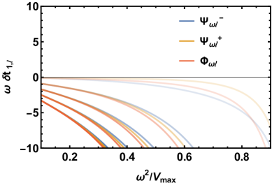
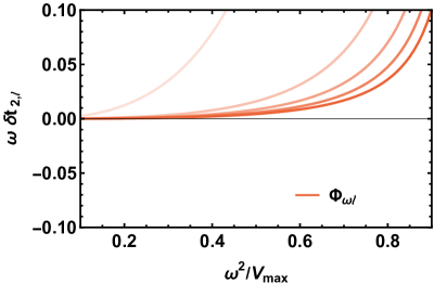
Figure 1: sGB corrections on the time delays for modes of different frequency $\omega$ and degree $\ell$. Here $V_{\rm max}$ is the maximum of the corresponding GR potentials, and curves, from light to dark, represent modes with $\ell=2,22,42,62$ and $82$. The left panel shows the corrections from the $c_{1}$-term, while the right panel shows those from the $c_{2}$-term. As in Eqs. (7) and (8), the $c_{2}$-term only affects the scalar modes.

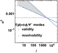
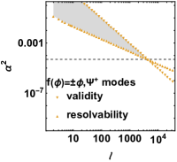
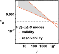
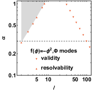
Figure 2: Causality violating regions (shadowed regions) in sGB gravity. The left three panels show the parameter spaces for $\Psi^{-}_{\omega\ell}$, $\Psi^{+}_{\omega\ell}$ and $\Phi_{\omega\ell}$ for the case of $|c_{1}|=1$ and $c_{2}=0$, and the most right panel shows the parameter space for $\Psi_{\omega\ell}$ for the case of $c_{1}=0$ and $c_{2}=-1$. A solid, up-pointing triangle denotes the resolvability condition for each $\ell$, while a solid, down-pointing triangle denotes the validity condition. The dashed lines denote the upper bounds on $\alpha^{2}$ or $\alpha$ imposed by infrared causality.

With Eqs. (7) and (8), we can discuss wave scattering and compute the resulting phase shift and time delay. For practical reasons, we shall focus on waves with $\gamma\equiv\omega^{2}/V_{\mathrm{max}}<1$, where $V_{\mathrm{max}}$ denotes the maximum of the corresponding GR potential, i.e., $V_{\rm GR}^{\pm}$ or $V_{\rm GR}$, depending on the modes considered. Taking the scalar modes for example, the asymptotical scattering solution at spatial infinity generally consists of an incident wave and a reflective wave,

$$\Phi_{\omega\ell}\propto e^{-i\omega r_{*}}+\mathcal{R}_{\omega\ell}e^{2i\delta_{\omega\ell}}e^{i\omega r_{*}},$$ (9)

where $\mathcal{R}_{\omega\ell}$ denotes the reflectivity, and $\delta_{\omega\ell}$ is the scattering phase shift. For $\omega<\left|V_{\mathrm{max}}\right|^{1/2}$, the phase shift can be calculated with the WKB approximation,

$$\delta_{\omega\ell}\simeq \int_{r_{*}^{T}}^{\infty}\mathrm{d}r_{*}\left(\sqrt{\omega^{2}-V_{\mathrm{GR}}-\alpha c_{2}V_{1}-\alpha^{2}c_{1}^{2}V_{2}}-\omega\right)$$

$$-\omega r_{*}^{T}-\frac{\pi}{4},$$ (10)

where $r^{T}_{*}$ is the turning point in the tortoise coordinate defined by $\omega^{2}-V_{\mathrm{GR}}-\alpha c_{2}V_{1}-\alpha^{2}c_{1}^{2}V_{2}=0$.

Given the phase shift, one can further define the time delay

$$\Delta T_{\ell}=2\frac{\partial\delta_{\omega\ell}}{\partial\omega},$$ (11)

which, in GR, is known as the Eisenbud-Wigner time delay [107]. According to the prescription of infrared causality [49, 50], we are interested in extracting the time delay arising from the corrections from the sGB EFT couplings, which is the total time delay subtracted by the GR part,

$$\Delta T^{\mathrm{sGB}}_{\ell}=\Delta T_{\ell}-\Delta T^{\mathrm{GR}}_{\ell}.$$ (12)

To the leading orders, we expect that

$$\Delta T^{\mathrm{sGB}}_{\ell}\simeq\alpha c_{2}\delta t_{2,\ell}+\alpha^{2}c_{1}^{2}\delta t_{1,\ell}.$$ (13)

According to Eqs. (III) and (11), we can analytically express $\delta t_{1,\ell}$ and $\delta t_{2,\ell}$ in terms of integrals, the explicit expressions of which are given in Appendix B. By numerical integration, we can get the results of $\delta t_{1,\ell}$ and $\delta t_{2,\ell}$. Similar discussions on the phase shift and time delay are also applied to the spin-2 modes. In Fig. 1, we show the numerical results of the sGB corrections on the time delays for both scalar and spin-2 modes with different frequency $\omega$ and degree $\ell$.

IV Causality constraints

As shown in Fig. 1, with some choices of $c_{1}$ and $c_{2}$, the sGB corrections on the time delay can be negative, i.e., $\Delta T^{\rm sGB}_{\ell}<0$. As stated previously in the introduction, a negative $\Delta T^{\rm sGB}_{\ell}$ indicates that the low energy modes, in our case the scattering waves, propagate outside the light cone set by the high energy modes. In particular, if the negative corrections on the time delay is resolvable, i.e., $-\Delta T^{\rm sGB}>\omega^{-1}$, it would imply violation of infrared causality [49, 50].

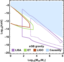
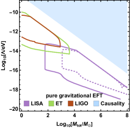
Figure 3: Detecablity of sGB gravity (left panel) and dim-6 pure gravitational EFT (right panel) with inspiral GWs from equal-mass binary BHs. $\Lambda$ is the EFT cutoff, and $M_{\rm tot}$ is the total mass of the binary. The shadowed regions show the parameter space allowed by infrared causality. We consider binaries insprialling at 300 Mpc with LIGO and 3Gpc with LISA, and 3Gpc (solid line) or 26 Gpc (dashed line) with Einstein Telescope (ET). For sGB gravity, we assume the dimensionless scalar charge difference is 1.

To be concrete, let us first consider sGB gravity with $c_{1}=0$ and $c_{2}\neq 0$, in which case the sGB coupling only affects the scalar modes up to $\mathcal{O}(\alpha)$ and $\Delta T^{\rm sGB}_{\ell}$ is negative whenever $c_{2}<0$. To carve out the boundary of the causality bounds, it is convenient to absorb $|c_{2}|$ in $\Lambda$ by setting $c_{2}=-1$. Then, the resolvability of $\Delta T^{\rm sGB}_{\ell}$ requires $\alpha\delta t_{2,\ell}<\omega^{-1}$. On the other hand, to ensure the EFT validity, the BH background and the scattering waves must be under control within the sGB EFT. In other words, all possible scalar quantities constructed in the system, e.g., by contracting on-shell momenta, Riemann tensors and their covariant derivatives, should be below the cutoff scale $\Lambda$. By applying power counting, it turns out for $\alpha\ll 1$, the EFT validity requires [50]

$$\alpha\ll\frac{\ell+\frac{1}{2}}{\omega^{2}G^{2}M^{2}}.$$ (14)

In Fig. 2, we show the constraints on $\alpha$ imposed by infrared causality, where a up-pointing triangle denotes the resolvability condition for each $\ell$, a down-pointing triangle denotes the validity condition, and the shadowed regions violate infrared causality. We consider waves with $\gamma=0.9$ such that we can get a relative tight constraints (cf. Fig. 1). From Fig. 2, we can conclude that infrared causality requires $\alpha\lesssim 0.3$ for sGB gravity with $c_{1}=0$ and $c_{2}=-1$.

Let us now consider sGB gravity with $c_{1}\neq 0$, in which case, the sGB coupling always leads to negative corrections on the time delay of the spin-2 modes; cf. Fig. 1 and Eq. (13). Then infrared acausality imposes

$$\frac{1}{-\omega\delta t_{1,\ell}}\lesssim c_{1}^{2}\alpha^{2}\ll\left(\frac{\ell+1/2}{\omega^{2}G^{2}M^{2}}\right)^{2},$$ (15)

where the lower bound is the resolvability condition, and the upper bound is the EFT validity condition. Moreover, one can also impose causality constraints on sGB gravity with $c_{1}\neq 0$ using the scalar modes. In this case, both the $c_{1}$- and $c_{2}$- term contribute, and it seems that a negative $c_{2}$ could improve the causality constraints derived from the scalar modes. However, assuming $c_{1}$ and $c_{2}$ to be ${\cal O}(1)$, the $c_{2}$-term does not affect the causality constraint very much due to a relative small $\delta t_{2,\ell}$. The results can be found in Fig. 2, which gives the bound $\alpha|c_{1}|\lesssim 0.005$, namely $\Lambda\gtrsim 6.3\times 10^{-10}\mathrm{eV}(3M_{\odot}/M)$, with $M_{\odot}$ being the mass of the sun, for sGB gravity with $c_{1}\neq 0$.

In the main text, we have focused on the sGB couplings (see Eq. (1)). Higher-dimensional operators from graviton self-interactions such as $R_{\mu\nu}{}^{\alpha\beta}R_{\alpha\beta}{}^{\gamma\sigma}R_{\gamma\sigma}{}^{\mu\nu}$ can actually lead to time delays at the same order as the linear sGB coupling. However, as we shall show in Appendix C, including the cubic curvature term only slightly modifies the causality constraint by tightening it to $\alpha|c_{1}|\lesssim 0.003$, namely $\Lambda\gtrsim 8.1\times 10^{-10}\mathrm{eV}(3M_{\odot}/M)$.

V Detectability of sGB gravity

With rapid advance in GW astronomy, we are interested in whether we can test consistent gravitational EFTs with GW observations, taking into account the causality constraints derived above. Before discussing the observability of sGB gravity, we first briefly review the interplay between causality bounds and GW experiments for the pure gravitational EFT (without the scalar field) [70]. As pointed out in Ref. [70], causality constraints require that the dim-6 cubic operator $R_{\mu\nu}{}^{\alpha\beta}R_{\alpha\beta}{}^{\gamma\sigma}R_{\gamma\sigma}{}^{\mu\nu}$ can not be tested with GW signals in the near future. For the ringdown tests, the leading order EFT corrections, e.g., on the BH quasi-normal modes are proportional to $(GM\Lambda)^{-4}$, which has to be small for the EFT to be valid on the BH horizon scale. Therefore, this dim-6 operator can hardly be tested with the BH ringdown waveforms given the precision of current GW observations. Nevertheless, the EFT with a lower cutoff might still be tested with early inspirals. For an EFT cutoff $\Lambda$, one can consider a period of inspiral with an orbital separation larger than $R_{\rm min}$. In this case, $R_{\mathrm{min}}$ is usually larger than the radius of the innermost stable circular orbit. Although the EFT corrections from the cubic curvature operator on the inspiral waveform are still proportional to $(GM_{\mathrm{tot}}\Lambda)^{-4}$, where $M_{\mathrm{tot}}$ is the total mass of the binary, it only requires $(\Lambda R_{\rm min})^{-1}\ll 1$ for the EFT to be valid for describing such a period of inspiral. $(GM_{\mathrm{tot}}\Lambda)^{-4}$ can still be considerable given that $R_{\rm min}/GM_{\mathrm{tot}}$ is large in early inspirals. However, causality imposes another condition besides the EFT validity. In particular, by considering a fiducial black hole of mass $R_{\rm min}/G$, causality requires $(\Lambda R_{\rm min})^{-4}<1.3\times 10^{-5}$ for the dim-6 pure gravitational EFT. As shown in the right panel of Fig. 3, such causality constraints are so strong that they eliminate all of the parameter space for testing the pure gravitational EFT with early inspirals.

Now, we consider testing sGB gravity with binary BH inspirals. The monopole charge of the hairy BH can lead to emission of scalar dipole radiation. As a result, in the Post-Newtonian (PN) expansions, the sGB corrections start from the $-1$PN order in the GW phases of binary BH inspirals [23],

$$\delta\psi_{\mathrm{sGB}}(f)=\beta_{\mathrm{sGB}}\left(GM_{\text{tot}}\Lambda\right)^{-4}\left(GM_{\rm tot}\pi f\right)^{-\frac{7}{3}},$$ (16)

where $f$ is the GW frequency. $\beta_{\mathrm{sGB}}$ is a dimensionless coefficient representing the scalar charge difference between the two BHs, the explicit expression of which is given in Appendix D. To estimate the observability of the EFT corrections, we calculate the accumulated phase shift $\Delta\psi_{\mathrm{sGB}}$ caused by the sGB couplings during the inspiral,

$$\Delta\psi_{\mathrm{sGB}}=\left|\delta\psi_{\mathrm{sGB}}\left(f_{\mathrm{max}}\right)-\delta\psi_{\mathrm{sGB}}\left(f_{\mathrm{min}}\right)\right|,$$ (17)

where $f_{\mathrm{max}}$ and $f_{\mathrm{min}}$ are the maximal and minimal frequencies of the inspiral signal. We only consider a period of inspiral where the GW frequency is lower than a cutoff frequency $f_{\rm cut}$ defined by $f_{\rm cut}=\Lambda^{2}R_{\rm min}$, so that the EFT is valid during such a period of inspiral [69]. For more details see Appendix D. The results are shown in the left panel of Fig. 3, where the contours show $\Delta\psi_{\mathrm{sGB}}\sim{\cal O}(1)$, indicating that sGB gravity can be tested with in the parameter regime bounded by the contours. On the other hand, we also plot the causality constraints, shown by the shadowed blue region. As calculating GW waveforms in sGB gravity requiring knowledge of the BH solution, as in Ref. [23], the theory should be at least causal down to the scale of BH horizon, i.e., $(\Lambda GM_{\rm tot}/2)^{-1}<0.07$.

Due to the dipole radiation resulted from scalar monopole, the sGB coupling typically leads to larger observational effects comparing to the dim-6 curvature operator. As a result, unlike the pure gravitational EFT, sGB gravity can still be tested with GW inspirals, with causality constraints leaving a couple of small windows for this possibility.

Appendix A Black holes and black hole perturbations in sGB gravity

The equations of motion of $g_{\mu\nu}$ and $\phi$ from (1) can be written as

$$R_{\mu\nu} =\frac{1}{2}\partial_{\mu}\phi\partial_{\nu}\phi-\frac{4}{\Lambda^{2}}\left(P_{\mu\alpha\nu\beta}-\frac{g_{\mu\nu}}{2}P_{\alpha\beta}\right)\nabla^{\alpha}\nabla^{\beta}f,$$ (A18)

$$\square\phi =-\frac{1}{\Lambda^{2}}f^{\prime}(\phi)\mathcal{G},$$ (A19)

where $P_{\mu\nu\rho\sigma}=R_{\mu\nu\rho\sigma}-2g_{\mu[\rho}R_{\sigma]\nu}+2g_{\nu[\rho}R_{\sigma]\mu}+g_{\mu[\rho}g_{\sigma]\nu}R$ and $P_{\mu\nu}\equiv P^{\lambda}{}_{\mu\lambda\nu}$. Using the static and spherically symmetric ansatz, and solving Eqs. (A18) and (A19) order by order in $\alpha$, we can get

$$A_{1}(x) =\frac{\left(10x^{4}+130x^{3}+33x^{2}+24x-50\right)}{240x^{7}},$$ (A20)

$$B_{1}(x) =\frac{\left(60x^{5}+30x^{4}+260x^{3}+15x^{2}+12x-230\right)}{240x^{7}},$$ (A21)

$$\phi_{1}(x) =\frac{6x^{2}+3x+2}{6x^{3}},$$ (A22)

$$\phi_{2}(x) =\frac{4380x^{5}+2190x^{4}+1460x^{3}+1095x^{2}+336x+100}{3600x^{6}},$$ (A23)

where $x=r/r_{g}$ with $r_{g}=2GM$.

Next, we derive the master equations for metric and scalar perturbations on the BH background. To that end, we consider the metric perturbations $h_{\mu\nu}$

$$g_{\mu\nu}=\bar{g}_{\mu\nu}+h_{\mu\nu},$$ (A24)

and the the scalar perturbations $\delta\phi$

$$\phi=\bar{\phi}+\delta\phi,$$ (A25)

where $\bar{g}_{\mu\nu}$ and $\bar{\phi}$ are the background determined by Eqs. (4)-(6). The perturbation equations are obtained by substituting Eqs. (A24) and (A25) into Eqs. (A18) and (A19), and keeping the leading-orders of $h_{\mu\nu}$ and $\delta\phi$. The metric perturbations $h_{\mu\nu}$ can be split into a sum of odd-parity modes $h_{\mu\nu}^{-}$ and even-parity modes $h_{\mu\nu}^{+}$, while the scalar perturbations $\delta\phi$ are even-parity modes. We decompose the metric perturbations into tensor spherical harmonics in the frequency domain. Given the spherically symmetric background, there is no dependence on the order $m$, so we choose $m=0$ for simplicity. Also because of the spherical symmetry, modes of different degree $\ell$ decouple. In sGB gravity, since there is no parity-violation term, odd-parity modes and even-parity modes also decouple. In the Regge-Wheeler gauge, the metric perturbations of degree $\ell$ can be then written in matrix form as

$$h_{\mu\nu}^{-}=e^{-i\omega t}\left(\begin{array}[]{cccc}0&0&0&h_{0}\\ 0&0&0&h_{1}\\ 0&0&0&0\\ h_{0}&h_{1}&0&0\end{array}\right)\sin\theta Y_{\ell}^{\prime}(\theta),$$ (A26)

and

$$h_{\mu\nu}^{+}=e^{-i\omega t}\left(\begin{array}[]{cccc}AH_{0}&H_{1}&0&0\\ H_{1}&H_{2}/B&0&0\\ 0&0&r^{2}\mathcal{K}&0\\ 0&0&0&r^{2}\sin^{2}\theta\mathcal{K}\end{array}\right)Y_{\ell}(\theta)\text{, }$$ (A27)

while the scalar perturbations of degree $\ell$ can be written as

$$\delta\phi=e^{-i\omega t}\frac{\hat{\phi}}{r}Y_{\ell}(\theta),$$ (A28)

where $Y_{\ell}(\theta)=Y_{\ell 0}(\theta,\phi)$ are the spherical harmonics with $m=0$ and $h_{0},h_{1},H_{0},H_{1},H_{2},\mathcal{K}$ and $\hat{\phi}$ are functions of $r$. By substituting Eqs. (A26), (A27) and (A28) into the perturbation equations and considering the following definitions of master variables

$$\Psi^{\mathrm{-}}_{\omega\ell} =\frac{i\sqrt{AB}h_{1}}{r\omega}\bigg{[}1+\alpha^{2}c_{1}^{2}f_{h_{1}}\bigg{]},$$ (A29)

$$\tilde{\Psi}^{\mathrm{+}}_{\omega\ell} =\frac{1}{(J-2)r+3r_{g}}\left[-r^{2}\mathcal{K}\left(1+\alpha^{2}c_{1}^{2}f_{\mathcal{K}}\right)+\frac{i\sqrt{AB}rH_{1}}{\omega}\left(1+\alpha^{2}c_{1}^{2}f_{H_{1}}\right)\right],$$ (A30)

$$\tilde{\Phi}_{\omega\ell} =\left(1+\alpha^{2}c_{1}^{2}f_{\phi}\right)\hat{\phi},$$ (A31)

where $J=\ell(\ell+1)$ and

$$f_{h_{1}}= \frac{\left(4x^{3}+3x^{2}+3x-7\right)}{4x^{6}},$$ (A32)

$$f_{\mathcal{K}}= \frac{1}{19440x^{6}(3+(-2+J)x)^{2}}\bigg{[}-189540-486(-268+107J)x-162\left(-43-65J+14J^{2}\right)x^{2}$$

$$+27\left(5916+407J-332J^{2}+56J^{3}\right)x^{3}-45\left(2490-1877J+558J^{2}-204J^{3}+28J^{4}\right)x^{4}$$

$$+30\left(66+1679J-2872J^{2}+1824J^{3}-520J^{4}+56J^{5}\right)x^{5}$$

$$+90\left(-66-1619J+3698J^{2}-3260J^{3}+1432J^{4}-316J^{5}+28J^{6}\right)x^{6}$$

$$+40(-2+J)^{3}\left(-15-214J+252J^{2}-102J^{3}+14J^{4}\right)x^{7}\bigg{]}$$

$$-\frac{(-2+J)^{2}\left(-15-214J+252J^{2}-102J^{3}+14J^{4}\right)}{1458}\log\left[-2+J+\frac{3}{x}\right],$$ (A33)

$$f_{H_{1}}= -f_{\mathcal{K}},$$ (A34)

$$f_{\phi}= -\frac{1}{9720x^{6}\left[3+(-2+J)x\right]}\bigg{[}21870+162(-232+89J)x-81\left(99-10J+14J^{2}\right)x^{2}$$

$$+45\left(210+23J-74J^{2}+14J^{3}\right)x^{3}-30\left(-69-214J+252J^{2}-102J^{3}+14J^{4}\right)x^{4}$$

$$+30\left(30+413J-718J^{2}+456J^{3}-130J^{4}+14J^{5}\right)x^{5}$$

$$+20(-2+J)^{2}\left(-15-214J+252J^{2}-102J^{3}+14J^{4}\right)x^{6}\bigg{]}$$

$$+\frac{(-2+J)^{2}\left(-15-214J+252J^{2}-102J^{3}+14J^{4}\right)}{1458}\log\left[-2+J+\frac{3}{x}\right],$$ (A35)

we can get one master equation for $\Psi^{\mathrm{-}}_{\omega\ell}$

$$\frac{\mathrm{d}^{2}\Psi_{\omega\ell}^{-}}{\mathrm{d}r_{*}^{2}}+\left[\omega^{2}-V_{GR}^{-}-\alpha^{2}c_{1}^{2}V^{-}\right]\Psi_{\omega\ell}^{-}=0,$$ (A36)

and two coupled master equations for $\tilde{\Psi}_{\omega\ell}^{+}$ and $\tilde{\Phi}_{\omega\ell}$

$$\frac{\mathrm{d}^{2}\tilde{\Psi}_{\omega\ell}^{+}}{\mathrm{d}r_{*}^{2}}+\left[\omega^{2}-V_{\mathrm{GR}}^{+}-\alpha^{2}c_{1}^{2}V^{+}\right]\tilde{\Psi}_{\omega\ell}^{+}=A_{0}\left[\bigg{(}\alpha c_{1}p_{1}+\alpha^{2}c_{1}c_{2}p_{2}\bigg{)}\frac{\mathrm{d}\tilde{\Phi}_{\omega\ell}}{\mathrm{d}r_{*}}+\bigg{(}\alpha c_{1}q_{1}+\alpha^{2}c_{1}c_{2}q_{2}\bigg{)}\tilde{\Phi}_{\omega\ell}\right],$$ (A37)

$$\frac{\mathrm{d}^{2}\tilde{\Phi}_{\omega\ell}}{\mathrm{d}r_{*}^{2}}+\left[\omega^{2}-V_{\mathrm{GR},\ell}-\alpha c_{2}V_{1}-\alpha^{2}c_{1}^{2}V_{2}\right]\tilde{\Phi}_{\omega\ell}=A_{0}\left[\bigg{(}\alpha c_{1}j_{1}+\alpha^{2}c_{1}c_{2}j_{2}\bigg{)}\frac{\mathrm{d}\tilde{\Psi}_{\omega\ell}^{+}}{\mathrm{d}r_{*}}+\bigg{(}\alpha c_{1}n_{1}+\alpha^{2}c_{1}c_{2}n_{2}\bigg{)}\tilde{\Psi}_{\omega\ell}^{+}\right].$$ (A38)

Here the GR potentials are

$$V^{-}_{\text{GR}} =\frac{A_{0}}{r_{g}^{2}}\left(\frac{J}{x^{2}}-\frac{3}{x^{3}}\right),$$ (A39)

$$V^{+}_{\text{GR}} =\frac{A_{0}}{r_{g}^{2}}\left[\frac{(J-2)^{2}Jx^{3}+3(J-2)^{2}x^{2}+9(J-2)x+9}{x^{3}((J-2)x+3)^{2}}\right],$$ (A40)

$$V_{\text{GR}} =\frac{A_{0}}{r_{g}^{2}}\left(\frac{J}{x^{2}}+\frac{1}{x^{3}}\right),$$ (A41)

with $A_{0}=1-r_{g}/r$, and the corrections on the GR potentials are given by

$$V^{-}= \frac{1}{x^{5}}\bigg{\{}A_{0}\left(2x^{2}+3x+4\right)\omega^{2}+\frac{1}{3840r_{g}^{2}x^{5}}\bigg{[}2880x^{6}-160(71J-567)x^{5}+160(73J-774)x^{4}$$

$$+48(11J+745)x^{3}+384(61J-1472)x^{2}-32(685J-32631)x-491520\bigg{]}\bigg{\}},$$ (A42)

$$V^{+}= \frac{1}{60x^{5}\left[(J-2)x+3\right]^{2}}\bigg{\{}A_{0}\bigg{[}30(J-2)x^{5}+40\left(3J^{2}-10J+8\right)x^{4}+15\left(12J^{2}-3J-34\right)x^{3}$$

$$+6\left(40J^{2}+24J-43\right)x^{2}+18(85J-72)x+2520\bigg{]}\omega^{2}$$

$$+\frac{1}{4r_{g}^{2}x^{5}\left[(J-2)x+3\right]^{2}}\bigg{[}-60(J-2)^{3}(J+3)x^{10}-10(-2+J)^{3}(-558+149J+71J^{2})x^{9}$$

$$\left.+10(-2+J)^{2}(5474-2593J-296J^{2}+73J^{3})x^{8}\right.$$

$$\left.+(-440000+496528J-150096J^{2}-818J^{3}+3301J^{4}+33J^{5})x^{7}\right.$$

$$\left.+3(187080-193260J+68172J^{2}-7495J^{3}-2354J^{4}+728J^{5})x^{6}\right.$$

$$\left.+(-998886+1322140J-609218J^{2}+72345J^{3}+15298J^{4}-2090J^{5})x^{5}\right.$$

$$\left.-3(-611854+747511J-273510J^{2}+19934J^{3}+2740J^{4})x^{4}\right.$$

$$\left.+9(-198893+194136J-49416J^{2}+1750J^{3})x^{3}\right.$$

$$+54(10544-8985J+1450J^{2})x^{2}-54(-4379+220J)x-149040\bigg{]}\bigg{\}},$$ (A43)

$$V_{1}= -\frac{6A_{0}}{r_{g}^{2}x^{6}},$$ (A44)

$$V_{2}= \frac{1}{x^{5}\left[(J-2)x+3\right]}\left\{-2A_{0}\left(2+x\right)\omega^{2}+\frac{1}{240r_{g}^{2}x^{5}\left[(J-2)x+3\right]}\bigg{[}180(-2+J)^{3}x^{9}\right.$$

$$+10(-2+J)^{2}(60+J+J^{2})x^{8}+10(296-518J+339J^{2}-103J^{3}+13J^{4})x^{7}$$

$$+3(-680+1142J-828J^{2}+169J^{3}+11J^{4})x^{6}$$

$$+3(26354-45054J+26843J^{2}-6417J^{3}+488J^{4})x^{5}$$

$$+(-569782+740413J-318645J^{2}+48422J^{3}-1490J^{4})x^{4}$$

$$+(1496837-1437849J+401682J^{2}-28210J^{3})x^{3}$$

$$-6(319952-201575J+27185J^{2})x^{2}-18(-67579+20795J)x-304560\bigg{]}\bigg{\}}.$$ (A45)

The leading-order corrections to the radial sound speed of $\Psi_{\omega\ell}^{\pm}$ and $\Phi_{\omega\ell}$, namely $\Delta c_{s}^{\pm}\equiv(c_{s}^{\pm})^{2}-1$ and $\Delta c_{s}\equiv c_{s}^{2}-1$ respectively, are determined by the coefficients of $\omega^{2}$ in the potential corrections $V^{\pm}$ and $V_{2}$. Explicitly, they are given by

$$\Delta c_{s}^{-}= \frac{c_{1}^{2}}{x^{5}}A_{0}\left(2x^{2}+3x+4\right),$$ (A46)

$$\Delta c_{s}^{+}= \frac{c_{1}^{2}A_{0}}{60x^{5}\left[(J-2)x+3\right]^{2}}\bigg{[}30(J-2)x^{5}+40\left(3J^{2}-10J+8\right)x^{4}+15\left(12J^{2}-3J-34\right)x^{3}$$

$$+6\left(40J^{2}+24J-43\right)x^{2}+18(85J-72)x+2520\bigg{]},$$ (A47)

$$\Delta c_{s}= -2\frac{c_{1}^{2}A_{0}(x+2)}{x^{5}\left[(J-2)x+3\right]}.$$ (A48)

Note that all the corrections to the sound speed appear at least at $\mathcal{O}(\alpha^{2})$. The other coefficients in Eqs. (A37) and (A38) are as follows:

$$p_{1}= -6\frac{(J-2)x+2}{r_{g}x^{3}\left[(J-2)x+3\right]^{2}},$$ (A49)

$$p_{2}= -2\frac{8(J-2)x^{3}+(5J+8)x^{2}+4(J+1)x+10}{r_{g}x^{6}\left[(J-2)x+3\right]^{2}},$$ (A50)

$$q_{1}= \frac{3\left[2(J-2)x^{4}+3x^{3}J^{2}-4\right]x^{2}+2(J+10)x-9}{r_{g}^{2}x^{5}\left[(J-2)x+3\right]^{2}},$$ (A51)

$$q_{2}= \frac{1}{15r_{g}^{2}x^{8}((J-2)x+3)}\bigg{[}146(J-2)x^{6}+73(J-2)x^{5}-219x^{4}+(647J-1732)x^{3}+(1975+304J)x^{2}$$

$$+6(144+35J)x+930\bigg{]},$$ (A52)

$$j_{1}= -\frac{2(J-2)x^{3}+(J-2)x^{2}+3(4J-9)x+48}{r_{g}x^{5}\left[(J-2)x+3\right]},$$ (A53)

$$j_{2}= \frac{1}{60r_{g}x^{8}\left[(J-2)x+3\right]^{2}}\bigg{[}146(J-2)x^{7}+219x^{6}+60\left(3J^{2}+8J-28\right)x^{4}+30\left(3J^{2}+5J+62\right)x^{3}$$

$$+3\left(20J^{2}+28J-61\right)x^{2}+(1806-780J)x-2310\bigg{]},$$ (A54)

$$n_{1}= \frac{2(x+2)}{x^{3}}\omega^{2}+\frac{1}{x^{7}r_{g}^{2}((J-2)x+3)^{2}}\bigg{[}-(J-2)^{2}Jx^{5}+(J-2)^{2}\left(3J^{2}-7J-3\right)x^{4}$$

$$+\left(20J^{3}-83J^{2}+83J+6\right)x^{3}+\left(33J^{2}-33J-75\right)x^{2}-9(4J-25)x-144\bigg{]},$$ (A55)

$$n_{2}= \frac{1}{15x^{6}}\left(73x^{4}+146x^{3}+219x^{2}+112x+50\right)\omega^{2}+\frac{1}{30x^{10}r_{g}^{2}((J-2)x+3)^{2}}\bigg{[}-73(-2+J)^{2}Jx^{8}$$

$$-73(-2+J)^{2}(3+J)x^{7}+(438-1513J+2233J^{2}-1153J^{3}+180J^{4})x^{6}$$

$$+(-219+4247J-3887J^{2}+647J^{3}+90J^{4})x^{5}+(-4539-13J+253J^{2}+242J^{3}+60J^{4})x^{4}$$

$$+(11121-1381J-644J^{2}+410J^{3})x^{3}+3(-1111-554J+230J^{2})x^{2}+(198-630J)x-2790\bigg{]}.$$ (A56)

The main perturbation equations (A37) and (A38), as they stand, are coupled, which makes it difficult to solve them with the WKB method. To obtain the final decoupled master equations (7) and (8) from them, we define new master variables $\Psi^{+}_{\omega\ell}$ and $\Phi_{\omega\ell}$ as

$$\tilde{\Psi}^{+}_{\omega\ell}= \Psi^{+}_{\omega\ell}+\alpha\left(f_{1}\dot{\Phi}_{\omega\ell}+f_{2}\Phi_{\omega\ell}\right)+\alpha^{2}\left(g_{1}\dot{\Phi}_{\omega\ell}+g_{2}\Phi+g_{3}\dot{\Psi}^{+}_{\omega\ell}+g_{4}\Psi^{+}_{\omega\ell}\right),$$ (A57)

$$\tilde{\Phi}_{\omega\ell}= \Phi_{\omega\ell}+\alpha\left(f_{3}\dot{\Psi}^{+}_{\omega\ell}+f_{4}\Psi^{+}_{\omega\ell}\right)+\alpha^{2}\left(g_{5}\dot{\Psi}^{+}_{\omega\ell}+g_{6}\Psi^{+}_{\omega\ell}+g_{7}\dot{\Phi}_{\omega\ell}+g_{8}\Phi_{\omega\ell}\right),$$ (A58)

where a dot denotes a derivative with respect to $r_{*}$, and $f_{1-4}$ and $g_{1-8}$ are functions of $r$. Substituting these expressions into Eqs. (A37) and (A38) and expanding up to $\mathcal{O}(\alpha^{2})$, we will find second and third order $r_{*}$-derivatives of $\Phi_{\omega\ell}$ and $\Psi_{\omega\ell}^{+}$ in the EFT corrections. When $\alpha=0$, these higher order derivatives terms can always be expressed in terms of $\Phi_{\omega\ell}$ and $\dot{\Phi}_{\omega\ell}$ ($\Psi_{\omega\ell}$ and $\dot{\Psi}_{\omega\ell}$), so we can remove all the higher-order derivatives terms in $\mathcal{O}(\alpha)$ and $\mathcal{O}(\alpha^{2})$. Finally, it is easy to see that, to get Eqs. (7) and (8) up to $\mathcal{O}(\alpha^{2})$, $f_{1-4}$ and $g_{1-8}$ need to satisfy

$$\ddot{f_{1}}+2\dot{f_{2}}+\left(V_{\text{GR}}-V_{\text{GR}}^{+}\right)f_{1}= c_{1}A_{0}p_{1},$$ (A59)

$$\ddot{f_{2}}+2\left(V_{\text{GR}}-\omega^{2}\right)\dot{f_{1}}+\dot{V}_{\text{GR}}f_{1}+\left(V_{\text{GR}}-V_{\text{GR}}^{+}\right)f_{2}= c_{1}A_{0}q_{1},$$ (A60)

$$\ddot{f_{3}}+2\dot{f_{4}}+\left(V_{\text{GR}}^{+}-V_{\text{GR}}\right)f_{3}= c_{1}A_{0}j_{1},$$ (A61)

$$\ddot{f_{4}}+2\left(V_{\text{GR}}^{+}-\omega^{2}\right)\dot{f_{3}}+\dot{V}_{\text{GR}}f_{3}+\left(V_{\text{GR}}^{+}-V_{\text{GR}}\right)f_{4}= c_{1}A_{0}n_{1},$$ (A62)

$$\ddot{g_{1}}+2\dot{g_{2}}+\left(V_{\text{GR}}-V_{\text{GR}}^{+}\right)g_{1}= -c_{2}V_{1}f_{1}+c_{1}c_{2}A_{0}p_{2},$$ (A63)

$$\ddot{g_{2}}+2\left(V_{\text{GR}}-\omega^{2}\right)\dot{g_{1}}+\left(V_{\text{GR}}-V_{\text{GR}}^{+}\right)g_{2}+\dot{V}_{\text{GR}}g_{1}= -c_{2}\dot{V}_{1}f_{1}-c_{2}V_{1}\left(f_{2}+2\dot{f}_{1}\right)+c_{1}c_{2}A_{0}q_{2},$$ (A64)

$$\ddot{g}_{3}+2\dot{g}_{4}= c_{1}A_{0}q_{1}f_{3}+c_{1}A_{0}p_{1}\left(f_{4}+\dot{f}_{3}\right),$$ (A65)

$$\ddot{g}_{4}+2\left(V_{\text{GR}}^{+}-\omega^{2}\right)\dot{g}_{3}+\dot{V}_{\text{GR}}^{+}g_{3}= c_{1}A_{0}q_{1}f_{4}+c_{1}A_{0}p_{1}\left[\dot{f}_{4}-\left(\omega^{2}-V_{\text{GR}}^{+}\right)f_{3}\right],$$ (A66)

$$\ddot{g}_{5}-\left(V_{\text{GR}}-V^{+}_{\text{GR}}\right)g_{5}+2\dot{g}_{6}= c_{2}V_{1}f_{3}+c_{1}c_{2}A_{0}j_{2},$$ (A67)

$$\ddot{g}_{6}+2\left(V_{\text{GR}}^{+}-\omega^{2}\right)\dot{g}_{5}+\left(V^{+}_{\text{GR}}-V_{\text{GR}}\right)g_{6}+\dot{V}_{\text{GR}}^{+}g_{5}= c_{2}V_{1}f_{4}+c_{1}c_{2}n_{2},$$ (A68)

$$\ddot{g}_{7}+2\dot{g}_{8}= c_{1}A_{0}n_{1}f_{1}+c_{1}A_{0}j_{1}\left(f_{2}+\dot{f}_{1}\right),$$ (A69)

$$\ddot{g}_{8}+2\left(V_{\text{GR}}-\omega^{2}\right)\dot{g}_{7}+\dot{V}_{\text{GR}}g_{7}= c_{1}n_{1}f_{2}+c_{1}j_{1}\left[\dot{f}_{2}-\left(\omega^{2}-V_{\text{GR}}\right)f_{1}\right].$$ (A70)

Appendix B Calculating time delays

Let us take the scalar modes as an example to illustrate how to compute the time delay. (The computation for the EFT corrections on the time delay for the spin-2 modes is very similar.) According to Eqs. (III) and (11), given a fixed $\omega$ satisfying $\omega<\left|V_{\mathrm{max}}\right|^{1/2}$, the time delay can be derived analytically via the WKB approximation as

$$\Delta T_{\ell}=2\frac{\partial\delta_{\omega\ell}}{\partial\omega}=2\int_{r_{*}^{T}}^{\infty}\mathrm{d}r_{*}\left(\frac{2\omega-\alpha c_{2}\frac{\partial V_{1}}{\partial\omega}-\alpha^{2}c_{1}^{2}\frac{\partial V_{2}}{\partial\omega}}{2\sqrt{\omega^{2}-V_{\mathrm{GR}}-\alpha c_{2}V_{1}-\alpha^{2}c_{1}^{2}V_{2}}}-1\right)-2r_{*}^{T}.$$ (B71)

The GR time delay $\Delta T^{\mathrm{GR}}_{\ell}$ is

$$\Delta T^{\mathrm{GR}}_{\ell}=2\int_{r^{\text{T,GR}}}^{\infty}\frac{\mathrm{d}r}{A_{0}}\left(\frac{2\omega}{2\sqrt{\omega^{2}-V_{\mathrm{GR}}}}-1\right)-2r_{*}^{\text{T,GR}},$$ (B72)

where $r^{\text{T,GR}}$ is the GR turning point defined by $\omega^{2}-V_{\mathrm{GR}}=0$ and $r_{*}^{\text{T,GR}}$ is the GR tortoise coordinate. When $c_{2}=0$ and $c_{1}\neq 0$, we can derive $\delta t_{1,\ell}$ as [70, 50]

$$\delta t_{1,\ell}=-2\int_{r^{\text{T,GR}}}^{\infty}\mathrm{d}r\mathcal{A}\left(\frac{\delta\mathcal{A}_{1}}{\mathcal{A}^{\prime}}\right)^{\prime},$$ (B73)

where

$$\mathcal{A} \equiv\frac{\omega}{A_{0}\sqrt{\omega^{2}-V_{\mathrm{GR}}}},$$ (B74)

$$\delta\mathcal{A}_{1} \equiv\mathcal{A}\left[\frac{V_{1}}{2\left(\omega^{2}-V_{\mathrm{GR}}\right)}-\frac{1}{2\omega}\frac{\partial V_{1}}{\partial\omega}-\frac{\delta A}{A_{0}}\right],$$ (B75)

with

$$c_{1}^{2}\alpha^{2}\delta A\equiv\sqrt{(A_{0}+\alpha^{2}c_{1}^{2}A_{1})(B_{0}+\alpha^{2}c_{1}^{2}B_{1})}-A_{0}+\mathcal{O}(\alpha^{4}).$$ (B76)

Here a prime denotes differentiation with respect to $r$. Similarly, when $c_{1}=0$ and $c_{2}\neq 0$, we have

$$\delta t_{2,\ell}=-2\int_{r^{\text{T,GR}}}^{\infty}\mathrm{d}r\mathcal{A}\left(\frac{\delta\mathcal{A}_{2}}{\mathcal{A}^{\prime}}\right)^{\prime},$$ (B77)

where

$$\delta\mathcal{A}_{2}\equiv\mathcal{A}\frac{V_{2}}{2\left(\omega^{2}-V_{\mathrm{GR}}\right)}.$$ (B78)

Here we have made use of the fact that $V_{2}$ does not depend on $\omega$. Numerically integrating Eqs. (B73) and (B77), we can compute EFT corrections on the time delay for the scalar modes.

When $\omega>\left|V_{\mathrm{max}}\right|^{1/2}$, part of the waves will enter the BH horizon, instead of being scattered back to spatial infinity, in which case, no causality constraint can be derived. To see that, let us consider minimally-coupled photons and gravitational/scalar waves that travel radially outwards from a radius $r_{0}$ near the BH horizon to spatial infinity. One can define a new type of time delay by comparing the travelling time between them [50]. This results in the following time advance for the GWs, as compared to the photons,

$$\Delta T^{\pm}_{\mathrm{adv}}\sim\int_{r_{0}}^{\infty}\frac{\mathrm{d}r\Delta c_{s}^{\pm}}{2\left(1-\frac{r_{g}}{r}\right)},$$ (B79)

where $\Delta c_{s}^{\pm}$ represent the leading order EFT corrections to the radial sound speed of the GWs, and we have taken the limit $r_{0}\rightarrow r_{g}$. See Appendix A for the expression of $\Delta c_{s}^{\pm}$. For the scalar mode, there is no time advance at leading order due to its negative correction to its sound speed. Carrying out the integration in (B79) yields $\Delta T^{\pm}_{\mathrm{adv}}\sim 3\alpha^{2}c_{1}^{2}GM$. A resolvable time advance can be obtained if $3\alpha^{2}c_{1}^{2}GM>\omega^{-1}$. However, this is not allowed by the EFT validity. To see this, note that, given the validity condition $\omega\ll\Lambda^{2}r_{b}$, where $r_{b}\sim GM$ is the impact parameter, we get $\omega GM\ll\alpha^{-2}$. This contradicts the resolvable condition $3\alpha^{2}c_{1}^{2}GM\gtrsim\omega^{-1}$ if we assume $c_{1}\sim\mathcal{O}(1)$. Therefore, no causality constraint can be derived when $\omega>\left|V_{\mathrm{max}}\right|^{1/2}$.

Appendix C Including dim-6 cubic curvature operator

In this appendix, we consider the effects of further including higher-dimensional operators from graviton self-interactions on the causality bounds. On a Ricci-flat background, the leading order such operator is the cubic curvature term $R_{\mu\nu}{}^{\alpha\beta}R_{\alpha\beta}{}^{\gamma\sigma}R_{\gamma\sigma}{}^{\mu\nu}$, which contributes to the scattering time delay at $\mathcal{O}(\alpha^{2})$ [51]. Together with the sGB coupling with $f(\phi)=c_{1}\phi$, the total action can be written as

$$S=\frac{M_{\mathrm{Pl}}^{2}}{2}\int\mathrm{~{}d}^{4}x\sqrt{-g}\left[R-\frac{1}{2}\partial_{\mu}\phi\partial^{\mu}\phi+\frac{c_{1}}{\Lambda^{2}}\phi\mathcal{G}+\frac{b}{\Lambda^{4}}R_{\mu\nu}{}^{\alpha\beta}R_{\alpha\beta}{}^{\gamma\sigma}R_{\gamma\sigma}{}^{\mu\nu}\right],$$ (C80)

where $b$ is also a dimensionless coupling constant. If $b$ and $c_{1}$ are $\mathcal{O}(1)$, the two terms lead to comparable EFT corrections to the time delay for the spin-2 modes. The steps to calcuate the time delays are very much like those with only the sGB term, which will not be repeated here. In Fig. 4, we plot the results when both the sGB term and the cubic curvature term are included, setting $|b|=c_{1}^{2}=1$ for simplicity. We see that now causality requires $\alpha\lesssim 0.003$. So the inclusion of a comparable dim-6 cubic curvature operator merely improves the causality bounds.

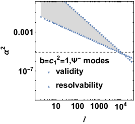
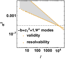
Figure 4: Causality violating regions (shadowed regions) in sGB gravity with the dim-6 cubic curvature operator included. The left and right panel show the parameter spaces for $\Psi^{-}_{\omega\ell}$, $\Psi^{+}_{\omega\ell}$ modes respectively. A solid, up-pointing triangle denotes the resolvability condition for each $\ell$, while a solid, down-pointing triangle denotes the validity condition. The dashed lines denote the upper bounds on $\alpha^{2}$.

Appendix D EFT corrections on inspiral phase

Here we provide slightly more details on how to compute the EFT corrections on the inspiral phase of binary BHs. As pointed out in [50, 69], EFT validity requires $f<\Lambda^{2}R_{\mathrm{min}}$. Here, according to the Kepler’s third law, we choose $R_{\mathrm{min}}^{3}=(\pi f)^{-2}GM_{\text{tot}}$. So the cutoff frequency $f_{\mathrm{cut}}$ is given by

$$f<f_{\mathrm{cut}}=\pi^{-\frac{2}{5}}\Lambda^{\frac{6}{5}}(GM_{\mathrm{tot}})^{\frac{1}{6}}.$$ (D81)

Given a binary BH with mass $M_{1}$ and $M_{2}$ for the two BHs, the coefficient $\beta_{\mathrm{sGB}}$ of the phase correction in Eq. (16) is given by [23]

$$\beta_{\mathrm{sGB}}=-\frac{5}{7168}\frac{\left(M_{1}^{2}\tilde{s}_{2}^{\mathrm{sGB}}-M_{2}^{2}\tilde{s}_{1}^{\mathrm{sGB}}\right)^{2}}{M_{\text{tot}}^{4}\eta^{18/5}}.$$ (D82)

Here $\mathcal{M}=(M_{1}M_{2})^{3/5}M_{\text{tot}}^{-1/5}$ is the chirp mass, $\eta=M_{1}M_{2}/M_{\text{tot}}^{2}$ is the symmetric mass ratio, and $\tilde{s}_{i}^{\mathrm{sGB}}=2(\sqrt{1-\chi_{i}^{2}}-1+\chi_{i}^{2})/\chi_{i}^{2}$ is the dimensionless scalar charge, where $\chi_{i}=\vec{S}_{i}\cdot\hat{L}/M_{i}^{2}$ is the projection of the spin angular momentum $\vec{S}_{i}$ in the direction of the orbital angular momentum $\hat{L}$. The inspiral frequency band $[f_{\mathrm{min}},f_{\mathrm{max}}]$ is determined by two aspects: the band depends on the capability of the GW detector, and the frequency should exceed neither the cutoff frequency nor the the innermost stable circular orbit frequency. The dimensionless charge $\tilde{s}_{i}^{\mathrm{sGB}}$ must be within the range $0\leq\tilde{s}_{i}^{\mathrm{sGB}}\leq 1$. In Fig. 3, to get a relatively large phase shift, we consider the case when $\tilde{s}_{1}^{\mathrm{sGB}}=1$ and $\tilde{s}_{2}^{\mathrm{sGB}}=0$.