Stability of non-minimally coupled dark energy in the geometrical trinity of gravity

Abstract

Within the geometrical trinity of gravity, we analyze scalar field dark energy models minimally and non-minimally coupled to gravity, postulating that a Yukawa-like interacting term is in form equivalent for general relativity, teleparallel and symmetric-teleparallel theories. Our analysis is pursued within two scalar field representations, where a quintessence and phantom pictures are associated with quasiquintessence and quasiphantom exotic fields. In the latter, we suggest how the phion-pressure can be built up without exhibiting a direct kinetic term. Accordingly, the stability analysis reveals that this quasiquintessence field provides a viable description of the universe indicating, when minimally coupled, how to unify dark energy and dark matter by showing an attractor point where $w_{\phi}=0$. Conversely, in the non-minimally coupling, the alternative field only leaves an attractor where dark energy dominates, mimicking de facto a cosmological constant behavior. A direct study is conducted comparing the standard case with the alternative one, overall concluding that the behavior of quintessence is well established across all the gravity scenarios. However, considering the phantom field non-minimal coupled to gravity, the results are inconclusive for power-law potentials in Einstein theory, and for the inverse square power potential in both teleparallel and symmetric-teleparallel theories.

I Introduction

The cosmological standard model is currently based on the $\Lambda$CDM background, in which a (bare) cosmological constant, $\Lambda$, drives the cosmic speed up SupernovaCosmologyProject:1998vns ; SupernovaCosmologyProject:1997zqe ; SupernovaSearchTeam:1998fmf ; Peebles:2002gy . The model appears particularly elegant, encompassing the majority of experimental tests Planck:2019nip ; Planck:2019evm ; Planck:2018nkj ; Planck:2018vyg ; Carloni:2024zpl , despite recently puzzled by rough evidences that may favor an evolving dark energy term DESI:2024mwx ; Zhao:2017cud ; Muccino:2020gqt ; Xu:2021xbt ; Copeland:2006wr ; Avsajanishvili:2023jcl ; Dunsby:2016lkw .

Accordingly, the revived interest in dark energy models, i.e., models in which dark energy is time-evolving may shed light on worrisome inconsistencies, such as cosmological tensions DiValentino:2021izs ; Bernal:2016gxb ; Vagnozzi:2019ezj ; Heymans:2020gsg ; KiDS:2020suj ; Hildebrandt:2018yau ; DiValentino:2017oaw , physical interpretations of $\Lambda$ Sakharov:1967pk ; Weinberg:2000yb ; Carroll:2000fy ; Dolgov:1997za ; Sahni:1999gb ; Straumann:1999ia ; Rugh:2000ji ; Padmanabhan:2002ji ; Yokoyama:2003ii ; Martin:2012bt , existence of early dark energy Poulin:2018cxd ; Karwal:2016vyq ; Sohail:2024oki , matching between dark energy and inflationary models Huterer:2002wf ; Yokoyama:2002ts ; Giare:2024akf ; Brax:2024rqs , and so forth, see e.g. Perivolaropoulos:2021jda ; Bull:2015stt ; Lynch:2024hzh ; zabat:2024wof ; Wang:2024dka ; Allali:2024cji ; Clifton:2024mdy ; Carrilho:2023qhq ; Lyu:2020lwm ; Wolf:2023uno .

In that matter, the preliminary release of the DESI collaboration has unexpectedly highlighted that a possible $w_{0}w_{a}$CDM model appears more compatible than the $\Lambda$CDM paradigm by considering new baryonic oscillation data catalogs DESI:2024mwx , by reinterpreting dark energy in terms of an evolving scalar field Copeland:2006wr .

In this respect, although theoretically well-established, non-minimally coupled scalar field dark energy scenarios have not been extensively explored at late-time Szydlowski:2008in ; Setare:2010pfa , but most of the analyses have been pursued at early times Kaiser:2015usz ; Ema:2017loe ; Bahamonde:2017ize ; DiValentino:2019jae .

However, recent inflationary results by the Planck satellite have shown that non-minimally coupling the scalar fields with curvature reliably enhances the viability of chaotic potentials that would otherwise be excluded Panotopoulos:2014hwa ; Nozariand:2015yfi ; Eshaghi:2015rta ; delCampo:2015wma ; Bostan:2023ped ; Kamali:2018ylz . Remarkably, in the context of Higgs inflation, a fourth order potential non-minimally coupled to the curvature leads to the Starobinsky potential, shifting to the Einstein frame Calmet:2016fsr ; Mantziris:2022fuu ; Mishra:2019ymr . To put into perspective, non-minimal couplings may help in both alleviating the cosmological tensions, being quite important even at late-time DiValentino:2019jae ; BarrosoVarela:2024htf and not only immediately after the Big Bang.

Hence, embracing the idea of exploring possible couplings between dark energy fields and curvature, at both late and intermediate times, would therefore open new avenues toward the fundamental properties related to dark energy, among which its evolution Capozziello:2022jbw , a possible interaction with other sectors, its form, and so on Farrar:2003uw ; Wang:2016lxa . Motivated by the above points, we here focus on scalar field dark energy models, minimally and non-minimally coupled. The couplings are thus performed within the so-called trinity of gravity BeltranJimenez:2019esp as cosmological backgrounds, highlighting the main differences when coupling dark energy with curvature, $R$, torsion, $T$, and non-metricity, $Q$, scalars. We explore six quintessence scenarios and five phantom potentials of dark energy, whose evolution has not been ruled out by observations yet, but rather can revive as due to the last findings presented by the DESI collaboration. For the sake of completeness, we additionally seek for dust-like scalar fields, namely for alternative version of scalar field description, that is divided into quasiquintessence and quasiphantom field Luongo:2023jnb , respectively. Precisely, in both the so-cited representations, we analyze the corresponding modified Friedmann equations and study the cosmological dynamics by computing autonomous systems of first-order differential equations. Reliably, in formulating the dynamical variables, in lieu of using the widely-used exponential and power-law potentials Copeland:2006wr ; Bahamonde:2017ize , whose advantage only lies in reducing the overall complexity, we select more appropriate dimensionless functions that may work regardless the types of involved potentials. To this end, we explore the critical exponents and fix the free parameters for each potential. Our main findings suggest that, under minimal coupling, the quasiquintessence model reveals a critical point where the universe behaves like dust. This critical point does not appear in the standard scalar field approach, indicating that an alternative framework, in the form of quasiquintessence, could properly unify dark energy and dark matter under the same scenario. This dust-like characteristic disappears when coupling is introduced, hiding the differences between the standard and alternative descriptions. Here, our results show that, while it is possible for dark energy to couple with curvature, torsion, or non-metricity scalars, not all the paradigms appear viable. Notably, in the phantom field scenario, numerical analysis yields inconclusive results for power-law potentials within the curvature-coupling framework. In contrast, only the inverse square potential is not supported in the teleparallel and symmetric-teleparallel dark energy.

The paper is structured as follows. In Sect. II, we introduce the non-minimally couplings within the geometrical trinity of gravity and analyze the modified cosmological equations. In Sect. III, we study the modified cosmological equations, and present the autonomous systems for both minimally and non-minimally coupled cosmologies. Last but not least, we also introduce all the potentials used for quintessence and phantom field. Then, in Sect. IV, we perform a stability analysis for the minimally and non-minimally coupled scenarios, identifying the critical points for all the potentials and computing the cosmological quantities within them. Finally, in Sect. V, we present the conclusions and perspectives of our work.

II Non-minimally couplings within the trinity of gravity

The geometrical trinity of gravity is ensured by the equivalence principle, leading to equivalent representations of Einstein’s field equations, albeit using different geometrical quantities to describe gravity, i.e., curvature, $R$, torsion, $T$, and non-metricity, $Q$, scalars.

Below we introduce the conformal non-minimal coupling between the scalar field, acting as dark energy, and gravity, under the form of $R,T$ and $Q$.

II.1 Background

At background, it would be convenient to set a general action, $\mathcal{S}$, depending on $R$, $T$ and $Q$, conventionally written as

$$\mathcal{S}=\int d^{4}x\sqrt{-g}\left[\frac{\mathcal{F}(U,\phi)}{2k^{2}}+\mathcal{L}_{m,r}+\mathcal{L}_{\phi}\right],$$ (1)

where $k^{2}=8\pi G$ and $\mathcal{F}(U,\phi)=U-k^{2}\xi U\phi^{2}$, whereas $U\equiv\{R,T,Q\}$. The former represents an auxiliary functional, depending on the scalar field and on the “gravity function”, identified in the set $U$. Clearly, $U$ singles out one type of gravitational interaction, among the three and, moreover, in $\mathcal{F}$, the coupling constant, $\xi$, represents the strength of the particular fifth force between $\phi$ and $U$. Accordingly, we implicitly refer to the tenet that, for $R,T$ and $Q$, the interaction strength remains unaltered.

Further, $\mathcal{L}_{m}$ and $\mathcal{L}_{\phi}$ denote the matter and scalar field sectors, respectively, indicating the kind of non-gravitational contributions entering the energy-momentum tensor.

We below derive the corresponding cosmological equations for a non-minimally coupled scalar field, exploring it within the framework of the geometrical trinity of gravity, adopting the spatially-flat version of the Friedmann-Robertson-Walker (FRW) metric,

$$ds^{2}=dt^{2}-a(t)^{2}(dr^{2}+r^{2}d\Omega^{2}),$$ (2)

where in the above-adopted radial coordinates, the angular part reads $d\Omega^{2}\equiv d\theta^{2}+\sin^{2}\theta d\phi^{2}$.

Under this scenario, as above claimed, we consider a dark energy field constructed by two different representations, i.e., the standard one and an alternative view, with the great advantage to mime dust, having that the sound speed identically vanishes Luongo:2018lgy ; Luongo:2024opv ; DAgostino:2022fcx ; Luongo:2023jnb .

II.2 Scalar field dark energy

As above claimed, it would be interesting to work two forms of scalar fields out, in order to describe dark energy.

We hereafter summarize them by:

• The Barrow representation, representing the standard scalar field picture, characterized by a density, $\rho_{\phi}$, and a pressure, $p_{\phi}$, is given by Copeland:2006wr

  $$\rho_{\phi}=\epsilon\frac{\dot{\phi}^{2}}{2}+V(\phi),\ p_{\phi}=\epsilon\frac{\dot{\phi}^{2}}{2}-V(\phi),$$ (3a)

  where conventionally $\epsilon=\pm 1$ denoting quintessence and phantom field, respectively.

• The alternative scalar field picture is given by Luongo:2018lgy ; DAgostino:2022fcx

  $$\rho_{\phi}=\epsilon\frac{\dot{\phi}^{2}}{2}+V(\phi),\ p_{\phi}=-V(\phi),$$ (4a)

  where $\epsilon=\pm 1$ indicates as above.

Both the representations are included by displaying the following generic Lagrangian,

$$\mathcal{L}=K-V(\phi)+\lambda Y[X,\nu(\phi)],$$ (5)

where $X\equiv\epsilon\frac{\dot{\phi}^{2}}{2}$ and $K\equiv K(X,\phi)$, while $\lambda$ is a Lagrange multiplier, i.e., zero for the standard case and nonzero for the alternative one Gao:2009me ; Luongo:2018lgy . Here, $\nu(\phi)$ represents the chemical potential and $Y$ a generic functional of it.

Thus, selecting $K=X$, from Eq. (5), and $\lambda=0$, for the standard case, we end up with

$$\mathcal{L}=\epsilon\frac{\dot{\phi}^{2}}{2}-V(\phi),$$ (6)

while, restoring $\lambda$, we obtain

$$\mathcal{L}=\epsilon\frac{\dot{\phi}^{2}}{2}-V(\phi)+\lambda Y,$$ (7)

that generically refers to the alternative description, yielding a quasiquintessence fluid when $\epsilon=+1$ and a quasiphantom fluid for $\epsilon=-1$.

To comprehend the idea behind the names quasiquintessence and quasiphantom, one can investigate the corresponding properties. In particular, the last form in Eq. (7), with $\epsilon=+1$, can be arguable either from modifying the Einstein equations by hand, see Ref. Gao:2009me , or by invoking an energy constraint imposed by virtue of $Y$ Luongo:2018lgy . The scenario yields a dust-like behavior of dark energy, in fact, from Eqs. (6) and (7), computing the sound speed, $c_{s}^{2}\equiv\frac{\partial p}{\partial\rho}$, we immediately find,

$$c_{s,Q}^{2} =\frac{\partial p_{\phi}}{\partial X}/\left(\frac{\partial\rho_{\phi}}{\partial X}\right)=1,$$ (8a)

$$c_{s,QQ}^{2} =\frac{\partial p_{\phi}}{\partial X}/\left(\frac{\partial\rho_{\phi}}{\partial X}\right)=0,$$ (8b)

respectively for quintessence, $c_{s,Q}$ and quasiquintessence, $c_{s,QQ}$. Interestingly, the same can be generalized for the quasiphantom case, by simply invoking $\epsilon=-1$ since the very beginning.

In the quintessence case, then, dark energy behaves as stiff matter, as the sound speed is unitary, i.e., resembles the speed of light, whereas in the quasiquintessence or quasiphantom cases, dark energy acts as a matter-like fluid, since the sound speed identically vanishes, as for dust DAgostino:2022fcx ; Luongo:2024opv .

In addition, under particular circumstances, the quasiquintessence naturally arises to heal the cosmological constant problem, as shown in Refs. Luongo:2018lgy ; Belfiglio:2023rxb , while being able to drive inflation as well, throughout the existence of a metastable phase, see Refs. DAgostino:2022fcx ; Luongo:2024opv .

II.3 Non-minimally coupled cosmology in Einstein’s theory

In general relativity, gravity is described with the scalar curvature, so we select $U=R$.

Considering here the non-minimal coupling scenario Nojiri:2006ri ; Sotiriou:2008rp ; DeFelice:2010aj ; Szydlowski:2008in ; Setare:2010pfa , the field equations obtained by varying the modified Hilbert-Einstein action in Eq. (1) with respect to a generic spacetime read

$$\begin{split}G_{\mu\nu}\mathcal{F}+\left(\partial_{\mu}\partial_{\nu}-g_{\mu\nu}\partial_{\mu}\partial^{\mu}\right)\mathcal{F}_{R}&-\frac{1}{2}g_{\mu\nu}\left[\mathcal{F}-R\mathcal{F}_{R}\right]\\ &=k^{2}\left(T^{(m)}_{\mu\nu}+T^{(\phi)}_{\mu\nu}\right).\end{split}$$ (9)

Here, $G_{\mu\nu}$ is the Einstein tensor, the subscript $R$ denote the derivatives with respect to the scalar curvature and $T^{(m)}_{\mu\nu}$ and $T^{(\phi)}_{\mu\nu}$ represent the energy-momentum tensor for matter and scalar field, respectively.

At this stage, assuming Eq. (2), we obtain the modified Friedmann equations, i.e.,

$$H^{2}=\frac{1}{3\mathcal{F}_{R}}\left(k^{2}\rho_{t}+\frac{R\mathcal{F}_{R}-\mathcal{F}}{2}-3H{\dot{\mathcal{F}}^{\prime}}\right),$$ (10)

$$2\dot{H}+3H^{2}=-\frac{k^{2}p_{t}+\ddot{\mathcal{F}}_{R}+2H\dot{\mathcal{F}}_{R}+(1/2)(\mathcal{F}-R\mathcal{F}_{R})}{\mathcal{F}_{R}},$$ (11)

in which $H=\frac{\dot{a}}{a}$ is the Hubble parameter, $\rho_{t}$ and $p_{t}$ are the total density and pressure, respectively given by: $\rho_{t}\equiv\rho_{\phi}+\rho_{m}$ and $p_{\phi}+p_{m}$, whereas the dot indicates the derivative with respect to the cosmic time $t$.

By substituting the explicit form of $\mathcal{F}\left(R,\phi\right)$ and recalling moreover that $R=6\left(\dot{H}+2H^{2}\right)$ in a homogeneous and isotropic universe Geng:2011aj , Eqs. (10) and (11) can be rewritten as

$$H^{2}=\frac{k^{2}}{3}\left(\rho^{\rm eff}_{\phi}+\rho_{m}\right),$$ (12)

$$2\dot{H}+3H^{2}=-k^{2}\left(p^{\rm eff}_{\phi}+p_{m}\right),$$ (13)

yielding the net effective density and pressure,

$$\rho^{\rm eff}_{\phi}=\rho_{\phi}+6\xi H\phi\dot{\phi}+3\xi H^{2}\phi^{2},$$ (14)

$$p^{\rm eff}_{\phi}=p_{\phi}-2\xi\phi\ddot{\phi}-2\xi\dot{\phi}^{2}-4H\xi\phi\dot{\phi}-\xi\left(2\dot{H}+3H^{2}\right)\phi^{2},$$ (15)

provided $\rho_{\phi}$ and $p_{\phi}$ from Eqs. (3a) and (4a), for both $\epsilon=\pm 1$.

Hence, by varying Eq. (1) with respect to the scalar field, we find two modified Klein-Gordon equations, both exhibiting a source term,

$$\ddot{\phi}+\frac{3}{\sigma}H\dot{\phi}+\epsilon V_{,\phi}=-6\epsilon\xi\left(\dot{H}+2H^{2}\right)\phi,$$ (16)

in which $\sigma=1$ and $\sigma=2$ select the kind of field, namely are given for Eqs. (3a) or Eq. (4a), respectively.

Remarkably, combining Eqs. (10) and (11) provides the Raychaudhuri equation,

$$\begin{split}\dot{H}&=-\frac{k^{2}}{1+\xi\left(6\xi-1\right)\left(k\phi\right)^{2}}\biggl{[}\left(\epsilon-2\sigma\xi\right)\frac{\dot{\phi}^{2}}{2\sigma}+4\xi H\phi\dot{\phi}\\ &+12\xi^{2}H^{2}\phi^{2}+\xi\phi\epsilon V_{,\phi}+\frac{(1+w_{m})}{2}\rho_{m}\biggr{]},\end{split}$$ (17)

where $w_{m}$ is conventionally the barotropic factor for matter.

II.4 Non-minimally teleparallel and symmetric-teleparellel cosmology

Compactly the non-minimally teleparallel and symmetric-teleparellel cases can be treated in the same way, from the mathematical viewpoint, once the coincidence gauge is optioned for the latter treatment BeltranJimenez:2017tkd . Even though aware of the conceptual difficulties related to the coincident gauge stability Heisenberg:2023wgk , we focus on this case only in order to show the formal degeneracy between $T$ and $Q$ in framing the non-minimal coupling.

Below we treat in detail both the cases.

The teleparallel case.

In teleparallel gravity Bahamonde:2021gfp ; Clifton:2011jh , the metric $g_{\mu\nu}$ is precisely expressed in terms of the vierbein field $e^{a}_{\mu}$ as $e^{a}_{\mu}e^{b}_{\nu}\eta_{ab}=g_{\mu\nu}$, with $\eta_{ab}=\text{diag}\left(1,-1,-1,-1\right)$, and $e=\text{det}\left(e^{a}_{\mu}\right)=\sqrt{-g}$.

Here, rather than relying on the torsion-free Levi-Civita connection characteristic of general relativity, the curvature-free Weitzenböck connection is employed. This connection introduces a non-zero torsion tensor, $\tensor{T}{{}^{\rho}_{\mu\nu}}$, and a corresponding contorsion tensor, $\tensor{K}{{}^{\mu\nu}_{\rho}}$, by

$$\tensor{T}{{}^{\rho}_{\mu\nu}}\equiv e^{\rho}_{a}\left(\partial_{\mu}e^{a}_{\nu}-\partial_{\nu}e^{a}_{\mu}\right),$$ (18)

$$\tensor{K}{{}^{\mu\nu}_{\rho}}\equiv-\frac{1}{2}\left(\tensor{T}{{}^{\mu\nu}_{\rho}}-\tensor{T}{{}^{\nu\mu}_{\rho}}-\tensor{T}{{}_{\rho}^{\mu\nu}}\right).$$ (19)

In teleparallel gravity, the Lagrangian density is characterized by the torsion scalar $T$, in contrast to $R$ used in general relativity. The torsion scalar $T$ is thus given by $T\equiv\tensor{S}{{}_{\rho}^{\mu\nu}}\tensor{T}{{}^{\rho}_{\mu\nu}}$, in which $\tensor{S}{{}_{\rho}^{\mu\nu}}\equiv\frac{1}{2}\left(\tensor{K}{{}^{\mu\nu}_{\rho}}+\delta^{\mu}_{\rho}\tensor{T}{{}^{\alpha\nu}_{\alpha}}-\delta^{\nu}_{\rho}\tensor{T}{{}^{\alpha\mu}_{\alpha}}\right)$. Then, by varying Eq. (1) with respect to the tetradal $e^{a}_{\nu}$, we end up with the modified Einstein’s equations

$$\begin{split}&e^{-1}\partial_{\mu}\left(ee^{\rho}_{a}\tensor{S}{{}_{\rho}^{\mu\nu}}\right)\mathcal{F}_{T}-e^{\lambda}_{a}\tensor{T}{{}^{\rho}_{\mu\lambda}}\tensor{S}{{}_{\rho}^{\nu\mu}}\mathcal{F}_{T}+e^{\rho}_{a}\tensor{S}{{}_{\rho}^{\mu\nu}}\partial_{\mu}(T)\mathcal{F}_{TT}\\ &+\frac{1}{4}e^{\nu}_{a}\mathcal{F}=\frac{k^{2}}{2}e^{\rho}_{a}\tensor{\left(T^{(m)}+T^{(\phi)}\right)}{{}_{\rho}^{\nu}},\end{split}$$ (20)

where the subscript $T$ represents the derivatives with respect to the torsion scalar.

With Eq. (2), the modified first Friedmann equations become Mirza:2017afs ; Geng:2011aj ; Gu:2012ww ,

$$6H^{2}\mathcal{F}_{T}+\frac{1}{2}\mathcal{F}=k^{2}\rho_{m},$$ (21)

$$2{\mathcal{F}}_{T}\left(3H^{2}-\dot{H}\right)+2H\dot{\mathcal{F}}_{T}+\frac{1}{2}\mathcal{F}=-k^{2}p_{m}.$$ (22)

Now, by substituting the explicit form of $\mathcal{F}$ and recalling that $T=-6H^{2}$ in the flat FRW metric, we can rewrite the above equations as

$$H^{2}=\frac{k^{2}}{3}\left(\rho^{\rm eff}_{\phi}+\rho_{m}\right),$$ (23)

$$2\dot{H}+3H^{2}=-k^{2}\left(p^{\rm eff}_{\phi}+p_{m}\right),$$ (24)

where the effective density and pressure for the scalar field are given by

$$\rho^{\rm eff}_{\phi}=\rho_{\phi}+3H^{2}\xi\phi^{2},$$ (25)

$$p^{\rm eff}_{\phi}=p_{\phi}-4H\xi\phi\dot{\phi}-\left(3H^{2}+2\dot{H}\right)\xi\phi^{2}.$$ (26)

Furthermore, by varying Eq. (1) with respect to the scalar field $\phi$, we get the modified Klein-Gordon equation

$$\ddot{\phi}+\frac{3}{\sigma}H\dot{\phi}+\epsilon V_{,\phi}=\epsilon 6H^{2}\xi\phi,$$ (27)

and by combining Eqs. (23) and (24), we obtain the explicit Raychaudhuri equation

$$\dot{H}=-\frac{k^{2}\left(\epsilon\frac{\dot{\phi}^{2}}{\sigma}-4H\xi\phi\dot{\phi}+\left(1+w_{m}\right)\rho_{m}\right)}{2\left(1-\xi k^{2}\phi^{2}\right)}.$$ (28)

The symmetric-teleparallel case.

All these equations are in form even valid for the non-minimally symmetric-teleparallel coupled cosmology, in the coincident gauge Carloni:2023egi ; Ghosh:2023amt ; BeltranJimenez:2017tkd , as stated in the beginning of this subsection. Particularly, in symmetric-teleparellel theory of gravity the connection is based only on the non-metricity, without any torsion Lu:2019hra ; Koussour:2023hgl . This implies that the connection is symmetric, and the torsion tensor vanishes, as well as the Riemann tensor. The non-metricity tensor, given by $Q_{\rho\mu\nu}=\nabla_{\rho}g_{\mu\nu}$, is used to write the disformation

$$L_{\rho\mu\nu}=\frac{1}{2}\left(Q_{\rho\mu\nu}-Q_{\mu\rho\nu}-Q_{\nu\rho\mu}\right),$$ (29)

a part of the general affine connection.

Here, we can derive the invariant, i.e., the non-metricity scalar,

$$Q=\frac{1}{2}P^{\rho\mu\nu}Q_{\rho\mu\nu},$$ (30)

where $P^{\rho\mu\nu}$ is called superpotential, provided by

$$P^{\rho\mu\nu}=L^{\rho\mu\nu}+\frac{1}{2}g^{\mu\nu}\left(\tilde{Q}^{\rho}-Q^{\rho}\right)+\frac{1}{4}\left(g^{\rho\mu}Q^{\nu}+g^{\rho\nu}Q^{\mu}\right),$$ (31)

with $\tilde{Q}_{\rho}\equiv\tensor{Q}{{}^{\mu}_{\mu\rho}}$ and $Q_{\rho}\equiv\tensor{Q}{{}_{\rho}^{\mu}{}_{\mu}}$, dubbed the non-metricity traces.

At this point, if we vary the action in Eq. (1) with respect to the metric, we infer

$$\begin{split}&\frac{2}{\sqrt{-g}}\nabla_{\rho}\left(\sqrt{-g}\mathcal{F}_{Q}\tensor{P}{{}^{\rho}_{\mu\nu}}\right)+\frac{1}{2}g_{\mu\nu}\mathcal{F}\\ &+\mathcal{F}_{Q}\left(P_{\mu\rho\alpha}\tensor{Q}{{}_{\nu}^{\rho\alpha}}-2Q_{\rho\alpha\mu}\tensor{P}{{}^{\rho\alpha}_{\nu}}\right)=k^{2}\left(T^{(m)}_{\mu\nu}+T^{(\phi)}_{\mu\nu}\right),\end{split}$$ (32)

where the subscript $Q$ indicates the derivatives with respect to the non-metricity scalar.

In the coincident gauge, the scalar acquires the simple form, $Q=-6H^{2}$ that appears formally equivalent to the torsion case, while “easier” than general relativity, for the absence of the dynamical term, $\sim\dot{H}$.

Consequently, we recover the same modified Friedmann equations along with the Klein-Gordon equation, as in the non-minimally teleparallel framework, namely Eqs. (23), (24) and (27).

III Phase-space analysis

The dynamics of dark energy models is here investigated through autonomous systems analysis. These systems are described by first-order differential equations without explicit time-dependent terms. Particularly, we focus on critical points and verify if they act as late-time attractors DAgostino:2018ngy ; Carloni:2023egi .

Accordingly, critical points are thus defined as solutions where the underlying differential equations vanish. In particular, they are dubbed attractors, if the system solutions asymptotically approach them.

As we can observe in the systems below, the framework in which we study dark energy and the potential considered is fundamental in determining the critical points and, then, the subsequent stability.

Hence, the following path is worked out.

• First, we analyze the generic case of minimally coupled cosmology with the alternative scalar field, including quasiquintessence and quasiphantom fields, performing a general approach in order to incorporate all the potentials. Here, the minimal coupling represents the limiting case for the non-minimally coupled framework, where $\xi\ll 1$, thus recovering the usual Friedmann equations. Afterwards, we compare the results obtained with those from the standard scalar field minimally coupled to gravity to identify the differences between the two descriptions. We here extend the overall analysis to all plausible dark energy potentials that still survive after the last findings on dark energy evolution.

• Second, we focus on systems non-minimally coupled to gravity. In this context, we examine the effects on the stability analysis when non-minimal coupling is introduced. Specifically, we introduce a Yukawa-like coupling, supposing its validity even in the framework of teleparallel and symmetric-teleparallel theory of gravity, i.e., not only in general relativity, see Ref. Capozziello:2024mxh . Here, the standard scalar field with our underlying potentials has not been analyzed deeply in the literature. Consequently, we work the stability out for both the standard and alternative scalar field formulations.

The potentials, considered below, being not ruled out from observations, are thus used in order to explain late-time dark energy phenomenology.

III.1 Quintessence-like potentials of dark energy

Regarding quintessence, the potentials studied are given below.

• Sugra potential. The simplest positive scalar potential model, derived from supergravity, is known as the Sugra potential and has the form

  $$V\left(\phi\right)=\frac{\Lambda^{4+\chi}}{\phi^{\chi}}e^{\gamma k^{2}\phi^{2}},$$ (33)

  with $\chi,\gamma>0$ . This potential form is often used to address the cosmological constant problem Martin:2012bt . In the context of quintessence, the equation of motion with this potential leads to tracker solutions Brax:1999yv ; Brax:1999gp ; Caldwell:2005tm .

• Barreriro-Copeland-Nunes potential: This is a double exponential potential defined as

  $$V(\phi)=\Lambda^{4}\left(e^{lk\phi}+e^{mk\phi}\right),$$ (34)

  where $l,m>0$ . In particular, a constraint arising from nucleosynthesis requires that $l>5.5$, while $m<0.8$ is needed to obtain a barotropic factor $w<-0.8$ in the quintessence scenario Barreiro:1999zs .

• Albrecht-Skordis potential: The Albrecht-Skordis potential takes the form

  $$V\left(\phi\right)=\Lambda^{4}\left(\left(k\phi-B\right)^{2}+A\right)e^{-\mu k\phi},$$ (35)

  where $A\geq 0$, $B\geq 0$ and $\mu>0$. It belongs to a class of scalar field models that may naturally arise from superstring theory, explaining the acceleration observed in the present epoch Albrecht:1999rm . Additionally, we include the case where $A=0$ and $B=0$, as described in supergravity models, see e.g. Ng:2001hs .

• Ureña-López-Matos potential: The quintessence potential given by

  $$V\left(\phi\right)=\Lambda^{4}\left(\sinh^{n}\left(\zeta k\phi\right)\right),$$ (36)

  where $\zeta>0$ and $n<0$, is denoted as Ureña-López-Matos potential.This potential acts as a tracker solution Urena-Lopez:2000ewq , which may have driven the universe into its current inflationary phase. The Ureña-López-Matos potential exhibits asymptotic behavior, resembling an inverse power-law potential in the early universe and transitioning to an exponential potential at late times.

• Inverse exponential potential: The inverse exponential potential assumes the form

  $$V\left(\phi\right)=\Lambda^{4}e^{\frac{1}{k\phi}},$$ (37)

  and it appears in Ref. Caldwell:2005tm , where it is proposed as a tracker model, without a zero minimum.

• Chang-Scherrer potential: The Chang potential is a modified exponential potential assuming the form

  $$V\left(\phi\right)=\Lambda^{4}\left(1+e^{-\tau k\phi}\right),$$ (38)

  where $\tau>0$. In contrast to models with a standard exponential potential, this approach even captures the features of early dark energy and may help to alleviate the coincidence problem, as shown in Ref. Chang:2016aex .

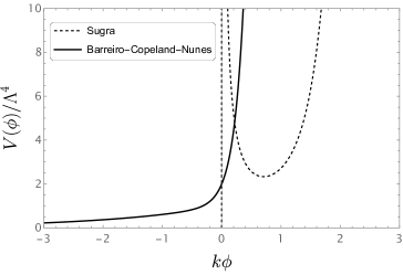
Figure 1: Behavior of quintessence potentials with fixed free parameters. The Sugra potential parameters are $\chi=1$ and $\gamma=1$, while the Barreiro-Copleand-Nunes ones are $m=6$ and $l=\frac{1}{2}$. The Sugra potential provides a significant contribution for both small and large field values, while the Barreiro-Copeland-Nunes potential is dominant for large field values only. For the Sugra potential, the offset is chosen as the Planck mass.

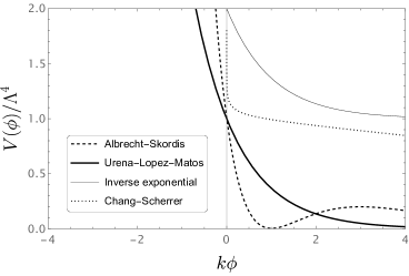
Figure 2: Behavior of quintessence potentials with fixed free parameters. The potential paremeters are given by: $A=0$, $B=0$ and $\mu=1$ for Albrecht-Skordis, $n=-\frac{1}{20}$ and $\zeta=1$ for Ureña-López-Matos, and $\tau=1$ for Chang-Scherrer. All the potentials exhibit the same decreasing behavior as the field value increases.

III.2 Phantom-like potentials of dark energy

Conversely to quintessence-like behavior, for phantom field, we employ the following potentials.

• Power law potential: The expression for this type of potential is given by

  $$V\left(\phi\right)=\Lambda^{4}\left(k\phi\right)^{\alpha},$$ (39)

  and these potentials are well fit by the $w_{0}w_{a}$ parametrization at redshifts $z\lesssim 1$, as reported in Ref. Scherrer:2008be ; Sami:2003xv . Power-law potentials are divided into two classes: those with $\alpha\geq 4$, which lead to ’Big Rip’ singularity, and those with $\alpha<4$, which avoid it. In our work, we study $\alpha=5,2,-2$, since they are not ruled out by observations.

• Exponential potential. It is the usual exponential potential, i.e.,

  $$V\left(\phi\right)=\Lambda^{4}e^{\beta k\phi},$$ (40)

  with $\beta>0$.This model, as for the power law potentials, is well approximates by the $w_{0}w_{a}$ parametrization, and it leads to a ’Big Rip’ singluarity Scherrer:2008be ; Sami:2003xv .

• Inverse hyperbolic cosine potential. The inverse hyperbolic cosine potential takes the following form

  $$V\left(\phi\right)=\Lambda^{4}\left(\cosh^{-1}\left(\alpha k\phi\right)\right),$$ (41)

  with $\alpha>0$. Here, the phantom field, when released from a point away from the origin with no initial kinetic energy, gravitates towards the peak of the potential, crosses it, and then reverses direction to undergo a damped oscillation around the potential’s maximum Singh:2003vx .

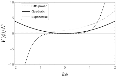
Figure 3: Behavior of phantom field potentials that increase as the field grows. The parameter value of the exponential potential is set to $\beta=1$. The fifth-power potential is the only one that allows negative values for the potential.

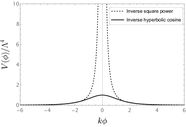
Figure 4: Behavior of phantom field potentials that decrease as the field increases. The inverse hyperbolic cosine potential is characterized by $\alpha=1$ and exhibits a peak at $\phi=0$.

Potential	Expression	$\lambda$	$\Gamma-1$
Type: Quintessence/Quasiquintessence
Sugra Avsajanishvili:2023jcl ; Brax:1999yv ; Brax:1999gp ; Caldwell:2005tm	$V\left(\phi\right)=\frac{\Lambda^{4+\chi}}{\phi^{\chi}}e^{\gamma k^{2}\phi^{2}}$	$-2\gamma k\phi+\frac{\chi}{k\phi}$	$\frac{4\gamma}{\lambda^{2}}+\frac{1}{\lambda k\phi}$
Barreiro-Copeland-Nunes Avsajanishvili:2023jcl ; Barreiro:1999zs	$V\left(\phi\right)=\Lambda^{4}\left(e^{lk\phi}+e^{mk\phi}\right)$	$-\frac{le^{lk\phi}+me^{mk\phi}}{e^{lk\phi}+e^{mk\phi}}$	$-\frac{(l+\lambda)(m+\lambda)}{\lambda^{2}}$
Albrecht-Skordis Avsajanishvili:2023jcl ; Albrecht:1999rm	$V\left(\phi\right)=\Lambda^{4}\left(\left(k\phi-B\right)^{2}+A\right)e^{-\mu k\phi}$	$\mu+\frac{2\left(B-k\phi\right)}{A+\left(B-k\phi\right)^{2}}$	$\frac{(\lambda-\mu)\left(\frac{1}{B-k\phi}-\lambda+\mu\right)}{\lambda^{2}}$
Ureña-López-Matos Avsajanishvili:2023jcl ; Urena-Lopez:2000ewq	$V\left(\phi\right)=\Lambda^{4}\left(\sinh^{n}\left(\zeta k\phi\right)\right)$	$-n\zeta\coth\left(\zeta k\phi\right)$	$-\frac{1}{n}+\frac{n\zeta^{2}}{\lambda^{2}}$
Inverse exponential Avsajanishvili:2023jcl ; Caldwell:2005tm	$V\left(\phi\right)=\Lambda^{4}e^{\frac{1}{k\phi}}$	$\frac{1}{\left(k\phi\right)^{2}}$	$\frac{2}{\sqrt{\lambda}}$
Chang-Scherrer Avsajanishvili:2023jcl ; Chang:2016aex	$V\left(\phi\right)=\Lambda^{4}\left(e^{-\tau k\phi}+1\right)$	$\frac{\tau}{1+e^{\tau k\phi}}$	$\frac{\tau}{\lambda}-1$
Type: Phantom/Quasiphantom field
Fifth power Avsajanishvili:2023jcl ; Scherrer:2008be	$V\left(\phi\right)=\Lambda^{4}\left(k\phi\right)^{5}$	$-\frac{5}{k\phi}$	$-\frac{1}{5}$
Inverse square power Avsajanishvili:2023jcl ; Scherrer:2008be	$V\left(\phi\right)=\Lambda^{4}\left(k\phi\right)^{-2}$	$\frac{2}{k\phi}$	$\frac{1}{2}$
Exponential Avsajanishvili:2023jcl ; Scherrer:2008be	$V\left(\phi\right)=\Lambda^{4}e^{\beta k\phi}$	$-\beta$	$0$
Quadratic Avsajanishvili:2023jcl ; Scherrer:2008be	$V\left(\phi\right)=\Lambda^{4}\left(k\phi\right)^{2}$	$-\frac{2}{k\phi}$	$-\frac{1}{2}$
Inverse hyperbolic cosine Avsajanishvili:2023jcl ; Singh:2003vx	$V\left(\phi\right)=\Lambda^{4}\left(\cosh^{-1}\left(\alpha k\phi\right)\right)$	$\alpha\tanh\left(\alpha k\phi\right)$	$1-\frac{\alpha^{2}}{\lambda^{2}}$

Table 1: Quintessence and phantom field potentials in minimally and non-minimally coupled cosmologies.

III.3 Minimally coupled cosmology

We analyze the dynamics of scalar field by rewriting the Klein-Gordon equation in terms of a set of dimensionless variables that, in general, are arbitrarily chosen.

In particular, to determine the dynamics of the scalar field, we might solve an autonomous system composed of first-order differential equations, involving dimensionless variables evolution.

In this subsection, we analyze the alternative scalar field description minimally coupled to gravity. To do so, we consider the dimensionless variables given by Gao:2009me ; Copeland:2006wr ; Bahamonde:2017ize

$$x\equiv\dfrac{k\dot{\phi}}{\sqrt{6}H}\,,\hskip 28.45274pty\equiv\dfrac{k\sqrt{V}}{\sqrt{3}H}\,,\hskip 28.45274ptv\equiv\frac{k\sqrt{\rho_{m}}}{\sqrt{3}H}\,,$$ (42)

$$\lambda\equiv-\dfrac{V_{,\phi}}{kV}\,,\hskip 28.45274pt\Gamma\equiv\dfrac{VV,_{\phi\phi}}{V_{,\phi}^{2}}\,.$$ (43)

The constraint equation in terms of these variables is rewritten as

$$1=\epsilon x^{2}+y^{2}+v^{2},$$ (44)

and the dark energy equation of state takes the following form $w_{\phi}=-\frac{y^{2}}{\epsilon x^{2}+y^{2}}$.

The presence of variable $\Gamma$ is fundamental if $\lambda$ is not a constant, so in the general case, the autonomous system reads

$$\begin{cases}x^{\prime}=-\frac{3}{2}xy^{2}+\epsilon\sqrt{\frac{3}{2}}\lambda y^{2},&\\ y^{\prime}=-\sqrt{\frac{3}{2}}\lambda xy+\frac{3}{2}y\left(1-y^{2}\right),&\\ \lambda^{\prime}=-\sqrt{6}f(\lambda)x,\end{cases}$$ (45)

where, prime represents derivatives with respect to the number of e-folding $N\equiv\ln a$ and $f(\lambda)=\lambda^{2}\left(\Gamma-1\right)$. The potentials that we want to analyze are resumed in Tab. 1. Here, we can see the explicit expression for $\lambda$ and $\Gamma-1$, i.e., to solve the system, we need to rewrite the function $\Gamma-1$ in terms of the dimensionless variable $\lambda$. We can also determine $\Gamma-1$ as a function of $\lambda$ for the Sugra and Albrecht-Skordis potentials. In this context, we derive the expressions that relate $u$ and $\lambda$, namely $u_{1,2}=\frac{\pm\sqrt{8\gamma\chi+\lambda^{2}}-\lambda}{4\gamma}$ for the Sugra potential and $u_{1,2}=\frac{\pm\sqrt{1-A(\lambda-\mu)^{2}}+B(\lambda-\mu)-1}{\lambda-\mu}$ for the Albrecht-Skordis potential. In the specific case of the Albrecht-Skordis potential where $A=B=0$, the parameter $\Gamma-1$ simplifies to $-(1+\mu/\lambda)^{2}/2$. Finally, after solving the system in Eq. (45), we can also obtain the evolution of matter by considering Eq. (44).

III.4 Non-minimally coupled cosmology

In the non-minimally coupled scenario, the Klein-Gordon equation has a source term, see Eq. (16), implying the presence of a new dimensionless variable, i.e., $u=k\phi$. Consequently, to find the dynamical behavior of a specific dark energy model, it may be convenient to introduce the following dimensionless variables

$$x\equiv\dfrac{k\dot{\phi}}{\sqrt{6}H}\,,\hskip 28.45274pty\equiv\dfrac{k\sqrt{V}}{\sqrt{3}H}\,,$$ (46)

$$v\equiv\dfrac{k\sqrt{\rho_{m}}}{\sqrt{3}H}\,,\hskip 28.45274ptu\equiv k\phi\,.$$ (47)

Even though these variables are the most prominent in the non-minimally coupled scenario DAgostino:2018ngy ; Carloni:2023egi , we here seek a more general approach characterizing all the critical points and stability, without fixing a potential a priori. To achieve it, we introduce a further term, $\lambda$, in the set of previous variables, including its evolution in the autonomous system. Accordingly, the model will influence the variables themselves plus the Klein-Gordon dynamics as, therein, it furnishes the term $V,_{\phi}$.

Adopting the above strategies, we can now explore how the underlying autonomous systems vary accordingly with a different choice of $U$, namely within the complete gravitational trinity of gravity.

III.4.1 Einstein theory

In the context of general relativity, employing the FRW curvature scalar, $R=6(\dot{H}+2H^{2})$, the constraint equation, Eq. (12), turns out to be

$$1=\epsilon x^{2}+y^{2}+v^{2}+2\sqrt{6}\xi ux+\xi u^{2},$$ (48)

and the parameter $s\equiv-\frac{\dot{H}}{H^{2}}$ is given by

$$\begin{split}s&=\frac{1}{1+\xi\left(6\xi-1\right)u^{2}}\biggl{[}\frac{3}{\sigma}\left(\epsilon-2\sigma\xi\right)x^{2}+4\sqrt{6}\xi xu+12\xi^{2}u^{2}\\ &-3\epsilon\xi\lambda uy^{2}+\frac{3\left(1+w_{m}\right)}{2}v^{2}\biggr{]},\end{split}$$ (49)

where, again, $\lambda=-\frac{V_{,\phi}}{kV}$. Thus, the system becomes

$$\begin{cases}x^{\prime}=(s-\frac{3}{\sigma})x+\sqrt{6}\epsilon\xi u\left(s-2\right)+\sqrt{\frac{3}{2}}\epsilon\lambda y^{2},&\\ y^{\prime}=sy-\sqrt{\frac{3}{2}}\lambda xy,&\\ u^{\prime}=\sqrt{6}x,&\\ \lambda^{\prime}=-\sqrt{6}f(\lambda)x.&\end{cases}$$ (50)

Again, for what concerns the evolution of matter, it can be derived by solving Eq. (48) and, in fact, from it, the dimensionless densities are determined as

$$\Omega_{m}=v^{2},\hskip 5.69054pt\Omega_{\phi}=\epsilon x^{2}+y^{2}+2\sqrt{6}\xi ux+\xi u^{2},$$ (51)

and the effective dark energy equation of state reads

$$\begin{split}w^{\rm eff}_{\phi}&=\frac{1}{{3\epsilon x^{2}+3y^{2}+6\sqrt{6}\xi xu+3\xi u^{2}}}\biggl{(}3\eta\epsilon x^{2}-3y^{2}\\ &-2\xi u\left(-3\sqrt{6}x+6\xi su-12\xi u+3\epsilon\lambda y^{2}\right)\\ &-12\xi x^{2}-4\sqrt{6}\xi xu-\xi\left(-2s+3\right)u^{2}\biggr{)},\end{split}$$ (52)

where $\eta=1,0$ for standard and alternative scalar field, respectively.

III.4.2 Teleparallel and symmetric-teleparallel theories

As already stressed, we remark that the non-minimally coupled symmetric-teleparallel picture is investigated imposing the coincident gauge, see Ref. BeltranJimenez:2017tkd . Then, these two descriptions of gravity can be unified under the same analysis since the scalar yields the same value in flat FRW, i.e., $T=Q=-6H^{2}$. Here, considering Eqs. (46)-(47), the constraint equation becomes

$$1=\epsilon x^{2}+y^{2}+v^{2}+\xi u^{2},$$ (53)

and the autonomous system is now rewritten in terms of these variables as

$$\begin{cases}x^{\prime}=(s-\frac{3}{\sigma})x+\epsilon\sqrt{6}\xi u+\sqrt{\frac{3}{2}}\epsilon\lambda y^{2},&\\ y^{\prime}=sy-\sqrt{\frac{3}{2}}\lambda xy,&\\ u^{\prime}=\sqrt{6}x,&\\ \lambda^{\prime}=-\sqrt{6}f(\lambda)x,&\end{cases}$$ (54)

where the parameter $s\equiv-\frac{\dot{H}}{H^{2}}$ acquires the form

$$s=\frac{\frac{3}{\sigma}\epsilon x^{2}-2\sqrt{6}\xi xu+\frac{3}{2}v^{2}}{1-\xi u^{2}}.$$ (55)

The effective dark energy equation of state becomes

$$w_{\phi}^{\rm eff}=\frac{\eta\epsilon x^{2}-y^{2}-\xi u^{2}+\frac{2}{3}\xi su^{2}-4\sqrt{\frac{2}{3}}\xi xu}{\epsilon x^{2}+y^{2}+\xi u^{2}}.$$ (56)

In addition, in view of the fact that Eq. (53) is different from Eq. (48), the dimensionless densities are now

$$\Omega_{m}=v^{2},\hskip 5.69054pt\Omega_{\phi}=\epsilon x^{2}+y^{2}+\xi u^{2}.$$ (57)

IV Stability analysis and physical results

In this section, we finally end up with the stability analysis of the above presented dark energy potentials for the different gravity scenarios, inside the gravitational trinity of gravity. Particularly, we look for the presence of attractors, that are specific critical points characterized by:

• Stable node, occurring if the eigenvalues of the Jacobian matrix are all negative.

• Stable spiral, arising if the real parts of the eigenvalues are negative and the determinant of the matrix computed at the critical point is negative.

In the opposite case, the critical point could be a saddle point, i.e., an unstable node or an unstable spiral.

More precisely, following Ref. Copeland:2006wr , we classify

• a saddle point to have at least one negative and one positive eigenvalue;

• a unstable node to have all positive eigenvalues;

• a unstable spiral to have critical points with eigenvalues that have positive real parts.

In all these cases, the point is called hyperbolic, and linear stability analysis is sufficient to determine its stability.

However, if one eigenvalue of the Jacobian matrix has a zero real part, the point is classified as non-hyperbolic, and different methods, beyond linear theory, are thus mandatory in order to determine the stability properties, since the linear theory alone fails to be predictive.

To address such conceptual issues, we apply the center manifold theory Boehmer:2011tp , and in case this approach would fail for specific potentials, we then resort to numerical simulations of the systems in Eqs. (45), (LABEL:eq:newdynsys) and (LABEL:eq:newdynsys1), essentially following the procedure underlined in Ref. Zhou:2007xp .

IV.1 Minimally coupled scenario

In this subsection, we apply the standard stability analysis technique, typically used in the context of a scalar field, to our alternative description, i.e., to quasiquintessence and quasiphantom fields. First, we identify the critical points of the system, and then we compute the eigenvalues at these points to assess stability.

The critical points for the alternative scalar field, minimally coupled with gravity, are detected by setting to zero the derivative with respect to $N$ of the $x$ and $y$ variables, if $\lambda=-\frac{V_{,\phi}}{kV}$ is constant.

Here, to study the dark energy dynamics, we analyze the small perturbations over these variables, i.e.,

$$\left(\begin{array}[]{c}\delta x^{\prime}\\ \delta y^{\prime}\\ \end{array}\right)={\mathcal{J}}\left(\begin{array}[]{c}\delta x\\ \delta y\\ \end{array}\right)\,,$$ (62)

where $\mathcal{J}$ is the Jacobian matrix.

Specifically, the small perturbations $\delta x$ and $\delta y$ are determined by the Jacobian matrix

$$\mathcal{J}=\left(\begin{array}[]{cc}\frac{\partial x^{\prime}}{\partial x}&\frac{\partial x^{\prime}}{\partial y}\\ \frac{\partial y^{\prime}}{\partial x}&\frac{\partial y^{\prime}}{\partial y}\\ \end{array}\right)_{(x=x_{c},y=y_{c})}\,,$$ (65)

in which $\textbf{X}_{c}=\left(x_{c},y_{c}\right)$ represents the critical point, indicated by the subscript $c$.

However, if $\lambda$ is no longer a constant, it is necessary to include it as well. Hence, Eq. (62) becomes

$$\left(\begin{array}[]{c}\delta x^{\prime}\\ \delta y^{\prime}\\ \delta\lambda^{\prime}\\ \end{array}\right)={\mathcal{J}}\left(\begin{array}[]{c}\delta x\\ \delta y\\ \delta\lambda\\ \end{array}\right)\,,$$ (72)

with $\mathcal{J}$ given by

$$\mathcal{J}=\left(\begin{array}[]{ccc}\frac{\partial x^{\prime}}{\partial x}&\frac{\partial x^{\prime}}{\partial y}&\frac{\partial x^{\prime}}{\partial\lambda}\\ \frac{\partial y^{\prime}}{\partial x}&\frac{\partial y^{\prime}}{\partial y}&\frac{\partial y^{\prime}}{\partial\lambda}\\ \frac{\partial\lambda^{\prime}}{\partial x}&\frac{\partial\lambda^{\prime}}{\partial y}&\frac{\partial\lambda^{\prime}}{\partial\lambda}\\ \end{array}\right)_{(x=x_{c},y=y_{c},\lambda=\lambda_{c})}\,,$$ (76)

where, this time, the critical point turns out to be $\textbf{X}_{c}=\left(x_{c},y_{c},\lambda_{c}\right)$.

Working this way, we then developed a general approach for the alternative scalar field scenarios, namely a treatment that turns out to be valid for all the types of involved potentials.

In addition, the above technique allows us to highlight the main expected differences among the standard and alternative descriptions of the scalar field Bahamonde:2017ize .

Precisely, the main difference is that, in the alternative scalar field case, there are two critical points where $\omega_{\phi}=0$, see Tab. 2. This implies that, as dynamics ends, dark energy mimes dust, physically interpreting the quasiquintessence field to behave as a unified dark energy-dark matter fluid at least for what concerns a pure dynamical perspective, as also confirmed in Ref. Gao:2009me , adopting a different path. Afterwards, to investigate the stability of the systems, it behooves us to study the eigenvalues computed at the critical points, as reported in Tab. 3.

Critical point	x	y	$\lambda$	Existence	$\omega_{\phi}$	Accel.	$\Omega_{\phi}$
$P_{0}$	0	0	Any	Always	$0$	No	0
$P_{1}$	Any	0	$\lambda_{*}$	$\lambda_{*}=0$	$0$	No	$\epsilon x^{2}$
$P_{2}$	Any	0	$\lambda_{*}$	$\lambda_{*}\neq 0$	$0$	No	$\epsilon x^{2}$
$P_{3}$	$\sqrt{2/3}\lambda_{*}$	$\sqrt{1-(2/3)\lambda_{*}^{2}}$	$\lambda_{*}$	$\lambda_{*}^{2}<3/2$	$-1+(4/3)\lambda^{2}_{*}$	$\lambda^{2}_{*}<\frac{1}{2}$	$1$
$P_{4}$	$0$	$1$	$0$	Always	$-1$	Yes	$1$

Table 2: The critical points of the system representing the alternative scalar field, minimally coupled to gravity, are given along with their existence conditions and cosmological values. The value $\lambda_{*}$ is any zero of the function $f(\lambda)=\lambda^{2}(\Gamma-1)$.

Point	Eigenvalues	Hyperbolicity	Stability
$P_{0}$	$\{0,0,3/2\}$	No	Unstable
$P_{1}$	$\{0,0,3/2\}$	No	Unstable
$P_{2}$	$\{0,-\sqrt{6}\lambda^{2}_{*}\Gamma^{\prime}_{*}x,3/2-\sqrt{3/2}\lambda_{*}x\}$	No	Indeterminate if $3/2-\sqrt{3/2}\lambda_{*}x<0$ and $\lambda^{2}_{*}\Gamma^{\prime}_{*}x\geq 0$
			Unstable if $3/2-\sqrt{3/2}\lambda_{*}x>0$ and $\lambda^{2}_{*}\Gamma^{\prime}_{*}x<0$
			Saddle if $3/2-\sqrt{3/2}\lambda_{*}x<0$ and $-\lambda^{2}_{*}\Gamma^{\prime}_{*}x>0$ or viceversa
$P_{3}$	$\{-2\lambda^{3}_{*}\Gamma^{\prime}_{*},-3/2+\lambda^{2}_{*},-3+2\lambda^{2}_{*}\}$	Yes	Stable if $-\sqrt{3/2}<\lambda_{*}<0$, $\Gamma_{*}^{\prime}<0$ or $0<\lambda_{*}<\sqrt{3/2}$, $\Gamma_{*}^{\prime}>0$
			Unstable if $\lambda_{*}<-\sqrt{3/2}$, $\Gamma_{*}^{\prime}>0$ or $\lambda_{*}>\sqrt{3/2}$, $\Gamma_{*}^{\prime}<0$
			Saddle otherwise
$P_{4}$	$\left\{-3,-\frac{3}{4}-\sqrt{\frac{9}{16}-3f(0)},-\frac{3}{4}+\sqrt{\frac{9}{16}-3f(0)}\right\}$	Yes if $f(0)\neq 0$	Stable if $f(0)>0$
			Saddle if $f(0)<0$

Table 3: Stability properties of the critical points for the system representing the alternative scalar field, minimally coupled to gravity, are discussed.

We then observe that the non-hyperbolicity prevents us from determining the stability of points $P_{2}$ and $P_{4}$ when $\frac{3}{2}-\sqrt{\frac{3}{2}}\lambda_{*}x<0$ and $\lambda^{2}_{*}\Gamma^{\prime}_{*}x\geq 0$, and $f(0)=0$, respectively. Here, $\lambda_{*}$ is any zero of function $f(\lambda)=\lambda^{2}(\Gamma-1)$ and $\Gamma^{\prime}_{*}$ is the derivative of $\Gamma$ with respect $\lambda$ computed in $\lambda_{*}$.

Thus, to determine whether these points can be attractors for the system, we need to select a specific potential and assess the stability of the model under examination by applying center manifold theory or numerical analysis.

For what concerns the critical point $P_{2}$, the center manifold theory does not provide useful information for analyzing the behavior around the critical point, and we have to rely on numerical methods to establish whether the point is an attractor. It is important to note that if one or both of the eigenvalues are negative, the point cannot be an attractor and is classified as an unstable or saddle point, as for the Chang-Scherrer model. The condition on the free parameter for this potential ensures that at least one eigenvalue is positive. In contrast, for the Sugra potential, $\lambda_{*}$ is imaginary, which means that this critical point does not exist.

In addition, since the dimensionless scalar field density is modeled by $\Omega_{\phi}=\epsilon x^{2}$, the phantom field appears unphysical as it provides a negative density value.

Thus, the numerical techniques is applied for Barreiro-Copeland-Nunes, Albrecht-Skordis and Ureña-López-Matos potentials imposing $v_{\rm in}^{2}=0.999$ at $z=10^{2}$ as a realistic initial condition for matter, see Refs. Carloni:2023egi ; Xu:2012jf ; DAgostino:2018ngy .

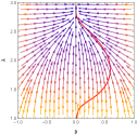
(a) Albreich-Skordis potential with free parametes set as $A=0$, $B=0$ and $\mu=3$.

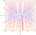
(b) Barreiro-Copeland-Nunes potential with free parameters set as $m=1/2$ and $l=6$.

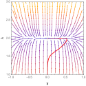
(c) Ureña-López-Matos potential with free parameters set as $n=-1$ and $\zeta=2$.

Figure 5: Phase-space trajectories on $y-\lambda$ plane for Albreicht-Skordis, Barreiro-Copeland-Nunes and Ureña-López-Matos potentials, where the red lines represent the solution of the dynamical systems. The initial conditions are set as $x_{\rm in}=0.03$, $y_{\rm in}=10^{-3}$ for all potentials, with $\lambda_{\rm in}=-7$ for the Barreiro-Copeland-Nunes potential and $\lambda_{\rm in}=1$ for the Albreicht-Skordis and Ureña-López-Matos potentials. From the numerical analysis, we observe that point $P_{2}$ is stable, i.e., an attractor, in all cases.

The dynamical system is then solved for each potential by setting $x_{\rm in}$, $y_{\rm in}$, and $\lambda_{\rm in}$ to ensure convergence to the critical point itself, and the results are displayed in Figs. 5(a), 5(b) and 5(c).

Thus, we can conclude that, for these potentials, the critical point, $P_{2}$, behaves as an attractor. This indicates a scenario where, within the critical point, dark energy may exhibit dark matter characteristics, i.e., dust-like properties, since the corresponding equation of state tends to vanish there.

At this stage, we subsequently analyze the critical point $P_{4}$. In the first instance, we observe that, if $\text{det}\mathcal{J}<0$ and $\frac{9}{16}-3f(0)<0$, the point is a stable spiral, yielding an attractor behavior. Conversely, if $f(0)=0$, the critical point is non-hyperbolic and, so, we require alternative techniques to study the stability. We first apply the center manifold theory, and the critical point point is an attractor if $\Gamma(0)>1$, as reported in Appendix A. However, if $\Gamma(0)$ diverges, we can not deduce anything about this point using the center manifold theory and we recur to numerical computation. This is the case of Inverse exponential and Chang-Scherrer potentials. Again, we use $v_{\rm in}^{2}=0.999$ at $z=10^{2}$ as realistic initial conditions to obtain the numerical solution, and the results are represented in Fig. 6. Then, we can conclude that, only for Barreiro-Copeland-Nunes, Ureña-López-Matos and Inverse hyperbolic cosine, the critical point $P_{4}$ is a saddle point, due to the fact that $f(0)<0$. For the other potentials, the critical point is an attractor in which dark energy behaves as a cosmological constant, dominating the universe.

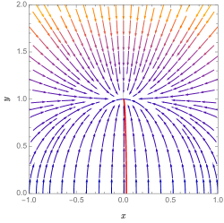
Figure 6: Phase-space trajectories on $x-y$ plane for Inverse exponential and Chang-Scherrer potentials, where the red line represents the solutions of the dynamical systems. The free parameter for the Chang-Scherrer potential is selected as $\tau=1$. The initial conditions are set as $x_{\rm in}=0.03$, $y_{\rm in}=10^{-3}$, and $\lambda_{\rm in}=10^{-10}$. Under these conditions, the solutions for the Inverse exponential and Chang-Scherrer potentials are identical, so they are represented on a single graph. Point $P_{4}$ is stable, i.e., an attractor, in both cases.

IV.2 Non-minimally coupled scenario

In this subsection, we analyze the stability of systems involving non-minimally coupled standard and alternative scalar field models, proposing a generalize approach to derive critical points without indicate the potential a priori. We obtain the same critical points for both the standard and alternative scalar field descriptions, indicating that the presence of coupling between dark energy and gravity unifies these two different types of scalar field. In particular, the dust-like behavior of the alternative scalar field disappears in favor of a typical dark energy description. To study the stability of these point, we study again the behavior of small perturbations. This time, the system has an additional variable due to the source term in the Klein-Gordon equation, so we consider the following linear evolution of perturbations

$$\left(\begin{array}[]{c}\delta x^{\prime}\\ \delta y^{\prime}\\ \delta u^{\prime}\\ \delta\lambda^{\prime}\\ \end{array}\right)={\mathcal{J}}\left(\begin{array}[]{c}\delta x\\ \delta y\\ \delta u\\ \delta\lambda\end{array}\right)\,,$$ (85)

with the Jacobian matrix determined as

$$\mathcal{J}=\left(\begin{array}[]{cccc}\frac{\partial x^{\prime}}{\partial x}&\frac{\partial x^{\prime}}{\partial y}&\frac{\partial x^{\prime}}{\partial u}&\frac{\partial x^{\prime}}{\partial\lambda}\\ \frac{\partial y^{\prime}}{\partial x}&\frac{\partial y^{\prime}}{\partial y}&\frac{\partial y^{\prime}}{\partial u}&\frac{\partial\lambda^{\prime}}{\partial\lambda}\\ \frac{\partial u^{\prime}}{\partial x}&\frac{\partial u^{\prime}}{\partial y}&\frac{\partial u^{\prime}}{\partial u}&\frac{\partial\lambda^{\prime}}{\partial\lambda}\\ \frac{\partial\lambda^{\prime}}{\partial x}&\frac{\partial\lambda^{\prime}}{\partial y}&\frac{\partial\lambda^{\prime}}{\partial u}&\frac{\partial\lambda^{\prime}}{\partial\lambda}\\ \end{array}\right)_{(x=x_{c},y=y_{c},u=u_{c},\lambda=\lambda_{c})}.$$ (90)

The critical points and corresponding eigenvalues for non-minimally coupled and teleparallel/symmetric-teleparallel dark energy are presented Tabs. 4-5 and 6-7, respectively. From these tables, we observe that the main difference between the gravity frameworks lies in the existence of a saddle critical point where dark energy behaves as radiation in non-minimally coupled dark energy, which is absent in both teleparallel and symmetric-teleparallel dark energy. This behavior is similar to the results found in Ref. Szydlowski:2013sma , albeit apparently it does not furnish new physics but just a convergence point.

Furthermore, as anticipated, the tables reveal no distinction between the standard and alternative descriptions of scalar field at critical points, since as stated above, the non-minimal coupling tends to hide the different characteristics of the potentials.

However, a subtle difference emerges when calculating the eigenvalues at the critical points, as shown in Tabs. 5 and 6. The linear stability analysis confirms that all the critical points are non-hyperbolic. The candidate attractor points are $P_{2}$, $P_{3}$, and $P_{4}$ for non-minimally coupled dark energy, and $P_{2}$ and $P_{3}$ for teleparallel and symmetric-teleparallel dark energy. Due to the large number of free parameters in this case, we perform a numerical analysis to determine the behavior of the dark energy systems.

In this respect, to numerically solve the systems, it is convenient to not consider the equation related to $\lambda^{\prime}$. In fact, by explicitly expressing the potential, we can rewrite $\lambda$ in terms of $u$, allowing us to solve each system with fewer variables. To evaluate the dynamics of dark energy, we assume that the universe is initially dominated by matter, setting $v^{2}_{\rm in}=0.999$ at $z=10^{2}$ Carloni:2023egi ; Xu:2012jf ; DAgostino:2018ngy . With this assumption, we let the system evolve by changing the potential and the initial conditions associated with it. In particular, the initial conditions are chosen in the range $y_{\rm in}\in[10^{-4},10^{-2}]$ and $u_{\rm in}\in[10^{-4},10^{-1}]$ to reach the convergence. Then, the value $x_{\rm in}$ is determined by solving the constraint equation. Among all the models, the only one that does not admit negative values of the field (i.e., negative values of $u$) is the fifth potential, as for such values, the potential becomes negative, leading to an imaginary dimensionless variable $y$.

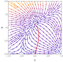
(a) Sugra with $\chi=1$, $\gamma=\frac{1}{2}$ and $\xi=-\frac{1}{2}$.

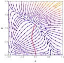
(b) Barreriro-Copeland-Nunes with $l=6$, $m=\frac{1}{2}$ ad $\xi=-1$.

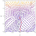
(c) Albrecht-Skordis with $A=B=\mu=\frac{1}{6}$ and $\xi=-\frac{1}{2}$.

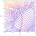
(d) Ureña-López-Matos with $n=-\frac{1}{2}$, $\zeta=\frac{1}{2}$ and $\xi=-\frac{1}{2}$.

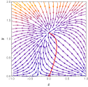
(e) Inverse exponential with $\xi=-\frac{1}{10}$.

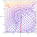
(f) Chang-Scherrer with $\tau=1$ and $\xi=-1$.

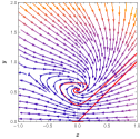
(g) Fifth power with $\xi=1$.

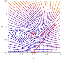
(h) Quadratic with $\xi=1$.

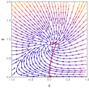
(i) Exponential with $\beta=1$ and $\xi=\frac{1}{2}$.

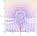
(j) Inverse hyperbolic cosine with $\alpha=1$ and $\xi=1$.

Figure 8: Phase-space trajectories on the $x-y$ plane for teleparallel and symmetric-teleparallel standard scalar field. The coupling constant and initial conditions are chosen to be valid for both the standard and alternative scalar field descriptions. Red lines indicate the solutions of the dynamical systems.

Finally, in Fig. 7 are prompted our findings for non-minimal coupled standard scalar field, while in Fig. 8 are displayed the results for teleparallel and symmetric-teleparallel standard scalar field in the coincident gauge. All these results are also valid for the alternative scalar field description, suggesting that the coupling between the scalar field and gravity masks the differences between the two types of scalar fields, as it dominates over the potentials themselves for given values of the field.

Critical point	x	y	u	$\lambda$	Existence	$\omega^{\rm eff}_{\phi}$	Accel.	$\Omega^{\rm eff}_{\phi}$
$P_{0}$	$0$	$0$	$\pm\sqrt{\frac{1}{\xi}}$	Any	$\xi>0$	$1/3$	No	$1$
$P_{1}$	$0$	$0$	$0$	Any	Always	$0/0$	Indeter.	$0$
$P_{2}$	$0$	$0<y^{2}<1$	$\pm\sqrt{\frac{1-y^{2}}{\xi+8\xi^{2}(\epsilon-1)}}$	$\pm\frac{4\xi}{y^{2}}\sqrt{\frac{1-y^{2}}{\xi+8\xi^{2}(\epsilon-1)}}$	for $\xi>0$ if $\epsilon=1$	$-1$	Yes	$\frac{8y^{2}\xi(\epsilon-1)+1}{8\xi(\epsilon-1)+1}$
					for $0<\xi<1/16$ if $\epsilon=-1$
$P_{3}$	$0$	$y^{2}>1$	$\pm\sqrt{\frac{1-y^{2}}{\xi+8\xi^{2}(\epsilon-1)}}$	$\pm\frac{4\xi}{y^{2}}\sqrt{\frac{1-y^{2}}{\xi+8\xi^{2}(\epsilon-1)}}$	for $\xi<0$ if $\epsilon=1$	$-1$	Yes	$\frac{8y^{2}\xi(\epsilon-1)+1}{8\xi(\epsilon-1)+1}$
					for $\xi<0$ or $\xi>1/16$ if $\epsilon=-1$
$P_{4}$	$0$	$1$	$0$	$0$	Always	$-1$	Yes	$1$

Table 4: Critical points of the system with existence condition and cosmological values for non-minimal coupling cosmology. These points are the same for the standard and alternative scalar field descriptions.

Point	Eigenvalues	Hyperbolicity	Stability
Standard scalar field
$P_{0}$	$\{0,\frac{3}{2},\frac{1}{4}(-3-\sqrt{9-48\epsilon\xi}),\frac{1}{4}(-3+\sqrt{9-48\epsilon\xi})\}$	No	Saddle
$P_{1}$	$\{-1,0,2,\epsilon\}$	No	Saddle
$P_{4}$	$\{-3,0,\frac{1}{2}(-3-\sqrt{9-48\epsilon\xi}),\frac{1}{2}(-3+\sqrt{9-48\epsilon\xi})\}$	No	Saddle if $\sqrt{9-48\epsilon\xi}>3$
			Indeterminate otherwise
Alternative scalar field
$P_{0}$	$\{0,\frac{3}{2},-i\sqrt{3\epsilon\xi},i\sqrt{3\epsilon\xi})\}$	No	Unstable
$P_{1}$	$\{0,2,\frac{1}{4}\left(-\sqrt{4\epsilon^{2}+20\epsilon+1}+2\epsilon+1\right),\frac{1}{4}\left(\sqrt{4\epsilon^{2}+20\epsilon+1}+2\epsilon+1\right)\}$	No	Saddle
$P_{4}$	$\{-3,0,\frac{1}{2}(-3-\sqrt{9-192\epsilon\xi}),\frac{1}{2}(-3+\sqrt{9-192\epsilon\xi})\}$	No	Saddle if $\sqrt{9-192\epsilon\xi}>3$
			Indeterminate otherwise

Table 5: Stability properties for the critical points of the non-minimal coupled standard scalar field system. The eigenvalues of $P_{2}$ and $P_{3}$ are of the same kind as $P_{4}$, but they depend on the explicit form of $y$ and $\Gamma$.

Critical point	x	y	u	$\lambda$	Existence	$\omega_{\phi}$	Accel.	$\Omega_{\phi}$
$P_{0}$	0	0	0	Any	Always	$0/0$	Indeterminate	0
$P_{1}$	0	$0<y^{2}\leq 1$	$\pm\sqrt{\frac{1-y^{2}}{\xi}}$	$\mp\frac{2\xi}{y^{2}}\sqrt{\frac{1-y^{2}}{\xi}}$	$\xi>0$	$-1$	Yes	$1$
$P_{2}$	0	$y^{2}>1$	$\pm\sqrt{\frac{1-y^{2}}{\xi}}$	$\mp\frac{2\xi}{y^{2}}\sqrt{\frac{1-y^{2}}{\xi}}$	$\xi<0$	$-1$	Yes	$1$
$P_{3}$	$0$	$1$	$0$	$0$	Always	$-1$	Yes	$1$

Table 6: Critical points of the teleparallel and symmetric-teleparallel dark energy systems with existence condition and cosmological values. These points are the same for the standard and alternative scalar field descriptions.

Point	Eigenvalues	Hyperbolicity	Stability
Standard scalar field
$P_{0}$	$\{0,\frac{3}{2},\frac{1}{4}\left(-3-\sqrt{9+96\xi\epsilon}\right),\frac{1}{4}\left(-3+\sqrt{9+96\xi\epsilon}\right)\}$	No	Saddle
$P_{3}$	$\{-3,0,\frac{1}{2}\left(-3-\sqrt{9+24\xi\epsilon}\right),\frac{1}{2}\left(-3+\sqrt{9+24\xi\epsilon}\right)\}$	No	Saddle if $\sqrt{9+24\xi\epsilon}>3$
			Indeterminate otherwise
Alternative scalar field
$P_{0}$	$\{0,\frac{3}{2},\sqrt{6\epsilon\xi},-\sqrt{6\epsilon\xi}\}$	No	Saddle
$P_{3}$	$\{-3,0,\frac{1}{4}\left(-3-\sqrt{3+96\xi\epsilon}\right),\frac{1}{4}\left(-3+\sqrt{3+96\xi\epsilon}\right)\}$	No	Saddle if $\sqrt{3+96\xi\epsilon}>3$
			Indeterminate otherwise

Table 7: Stability properties for the critical points of the teleparallel and symmetric-teleparallel dark energy systems. The eigenvalues of $P_{1}$ and $P_{2}$ are of the same kind as $P_{3}$, but they depend on the explicit form of $y$ and $\Gamma$.

V Outlooks and perspectives

Motivated by the revived interest in evolving dark energy models, as recently claimed by the DESI collaboration, we reconsidered whether minimal and non-minimal coupled scalar field dark energy models can suitably behave from a dynamical viewpoint. Particularly, the DESI collaboration has pointed out that an evolving dark energy contribution can be due to a unknown scalar field dynamics that, only in the simplest scenario, reduces to an effective $w_{0}w_{a}$CDM model DESI:2024mwx .

To this end, we computed the stability and the dynamical systems associated with the most popular forms of dark energy models, characterized by viable scalar field potentials.

Moreover, to extend the findings indicated by DESI, we did not limit our analysis to quintessence only, but considered phantom regimes, as well as alternative field representations, dubbed quasiquintessence and quasiphantom pictures, conceptually derived as possible generalizations of K-essence models, but with the great advantage to furnish an identically zero sound speed, namely behaving as dust-like fluids.

We provided, for the alternative scalar field representations, robust arguments in their favor, remarking their use to guarantee inflationary stability, or in erasing the excess of cosmological constant contribution throughout a metastable phase.

In addition, to check the goodness of each dark energy model, we ensured their suitability switching the theoretical background to alternatives to general relativity. To this end, we did not limit to Einstein’s theory, but explored the so-called geometrical trinity of gravity. Hence, we focused on general relativity first and then on its equivalent versions, offered by the teleparallel and symmetric-teleparallel formalism, by using as Lagrangian densities, $R,T$ and $Q$, respectively.

More in detail, for each gravitational background and for the set of dark energy potentials, we investigated minimal and non-minimal couplings between the scalar field and the gravity sector, adopting Yukawa-like interacting terms.

In so doing, we checked the main consequences of coupling dark energy with gravity, under the form of curvature, torsion or non-metricity and, moreover, in the case of non-minimal coupling, while the limiting case, $\xi\rightarrow 0$, leading to minimal coupling is also studied.

Nevertheless, even in the minimally coupled scenario, we developed a general approach to study the stability of the alternative scalar field. In particular, considering quasiquintessence, we discovered that there exists a critical point where dark energy exhibits dust-like characteristics. This is a non-hyperbolic point since one of the eigenvalues is zero, so we do not infer the stability limiting to the linear analysis. In this respect, we applied the center manifold theory and numerical methods, and, fixing free parameters, we conclude that it is an attractor for Albrecht-Skordis, Barreiro-Copeland-Nunes and Ureña-López-Matos potentials, suggesting that these potentials in the context of quasiquintessence determine a unified dark energy-dark matter fluid.

In addition, another critical point can be an attractor under specific conditions. This point is also given in the approach that generalizes stability for the standard scalar field, and it describes a scenario in which the universe is fully dominated by dark energy in the form of a bare cosmological constant, i.e., $w_{\phi}=-1$.

We extended the generalize method to study the stability in the context of non-minimal coupling scenarios, without expliciting the relation between $u$ and $\gamma$. Here, we analyzed the standard and alternative forms of the scalar field, both yielding the same critical points, contrary to the minimal coupled framework. This result indicates that the presence of coupling tends to hide the differences between these two scalar field descriptions, leading only a subtle differences in the form of eigenvalues. This finding confirms the results obtained for non-minimal couplings in inflationary regimes, suggesting that possible non-minimal couplings may be under different forms than Yukawa-like, but are in tension with the Higgs inflation and the Starobinky potential schemes, where, instead, the Yukawa-like term appears essential.

Moreover, with the given set of variables, all the critical points are non-hyperbolic, requiring a numerical approach to determine whether a critical point with three eigenvalues having negative real parts is an attractor. In any case, all points candidate as attractors lead to a universe dominated by dark energy under the form of a cosmological constant, and the unified dark energy-dark matter framework found in the minimimally coupled scenario is lost.

In the non-minimal usual general relativity framework, the phantom field power-law potentials are excluded from the analysis for both types of scalar fields, as they are ruled out by our computation.

Further, we analyzed teleparallel and symmetric-teleparallel dark energy within coincident gauge at the same time, by virtue of the mathematical degeneracy between the two frameworks.

Here, we derived again that the standard and alternative scalar field descriptions give the same results, leading to attractor points where dark energy dominates the universe with $w_{\phi}=-1$. Notably, in the case of teleparallel and symmetric-teleparallel dark energy, only for the inverse square power potential we did not find the correct conditions to determine the behaviour of critical point.

Thus, we can conclude that the quintessence and quasiquintessence models stand out as the most promising dark energy candidates, as they exhibit attractor points across all gravity scenarios considered.

In conclusion, we observe that:

• Quasiquintessence provides two interesting critical points in minimally coupled cosmology. One showing a unified dark energy-dark matter scenario, whereas the other leading to the standard framework, where dark energy dominates the universe under the form of a cosmological constant.

• The stability analysis in non-minimally coupled dark energy framework confirms that phantom fields are disfavored compared to quintessence, and this is confirmed for quasiphantom field too.

• For teleparallel and symmetric-teleparallel dark energy models, phantom fields are not fully-excluded, suggesting either the need for further investigation into the validity of Yukawa-like coupling in these gravity scenarios or possible differences among the background gravity theories.

Looking ahead, we will single out the best potentials exploring their consequences in various non-minimal coupling settings, utilizing the new releases from the DESI collaboration and investigating the growth of matter perturbations. Moreover, it would be interesting to study the same in the context where spatial curvature is not set to zero, to check if its influence is relevant. Last but not least, our approach would be useful to clarify whether these potentials can be even generalized for early dark energy contexts, in view of a possible resolution of the cosmological tensions Poulin:2018cxd ; Giare:2024akf .

Appendix A Center manifold theory

The non-hyperbolicity of a critical point arises when the Jacobian matrix, evaluated at that point, yields null eigenvalues. In such cases, the stability of the point cannot be determined using linear theory if all the non-zero eigenvalues have negative real parts. Thus, alternative techniques are needful, such as center manifold theory. This approach reduces the dimensionality of the system near the critical point, allowing the stability of the reduced system to be analyzed [116]. Below, we outline how the center manifold theory is applied throughout the text, following Ref. [122].

• We first rewrite the system in terms of new variables by shifting the critical point to the origin of phase-space.

• Second, the dynamical system is split into a linear and a nonlinear part, say

  $$q^{\prime}=Aq+f(q,p),$$ (91)

  $$p^{\prime}=Bp+g(q,p),$$ (92)

  where $(q,p)\in\mathbb{R}^{c}\times\mathbb{R}^{s}$, whereas the functions $f$ and $g$ satisfy the conditions

  $$f(0,0)=0,\quad Df(0,0)=0,$$ (93)

  $$g(0,0)=0,\quad Dg(0,0)=0.$$ (94)

  Here, the critical point is at the origin, with $Df$ denoting the matrix of first derivatives of $f$. The matrix $A$ is a $c\times c$ matrix whose eigenvalues have zero real parts, while $B$ is an $s\times s$ matrix with eigenvalues having negative real parts.

  If the system is not in this appropriate form, a further change of variables is performed, determing the eigenvectors and eigenvalues of the Jacobian matrix.

• Next, we introduce a function $h(q)$ and expand it in a Taylor series around the origin as $h(q)=aq^{2}+bq^{3}+\mathcal{O}(q^{4})$. The coefficients $a$ and $b$ are determined by solving the quasilinear partial differential equation

  $$Dh(q)(Aq+f(q,h(q)))-Bh(q)-g(q,h(q))=0,$$ (95)

  where $h(0)=Dh(0)=0$.

• Once the coefficients are determined, we can analyze the dynamics of the original system, restricted to the center manifold, by writing

  $$q^{\prime}=Aq+f(q,h(q)).$$ (96)

  If at least one of the coefficients is non-zero, this equation reduces to $q^{\prime}=\upsilon q^{n}$, where $\upsilon$ is a constant, and $n$ is a positive integer representing the lowest order in the expansion. If $\upsilon<0$ and $n$ is odd, the system is stable, and the critical point is an attractor. Otherwise, the critical point is unstable.

Now, we apply this technique to the critical point $P_{4}=(0,1,0)$, identified for the alternative scalar field model minimally coupled to gravity. We first shift the coordinates as $x=X$, $y-1=Y$, and $\lambda=\Lambda$, and rewrite the system in terms of these new variables. Thus, the dynamical system becomes

$$\begin{cases}&X^{\prime}=-\frac{3}{2}X(Y-1)^{2}+\epsilon\sqrt{\frac{3}{2}}\Lambda(Y-1)^{2},\\ &Y^{\prime}=-\sqrt{\frac{3}{2}}\lambda X(Y-1)+\frac{3}{2}(Y-1)\left(1-(Y-1)^{2}\right),\\ &\Lambda^{\prime}=-\sqrt{6}\Lambda^{2}\left(\Gamma(\Lambda)-1\right)X.\end{cases}$$ (97)

We compute the eigenvector matrix of the new system’s Jacobian and introduce a new set of coordinates as follows

$$\begin{pmatrix}v\\ w\\ z\end{pmatrix}=\begin{pmatrix}0&1&0\\ 1&0&-\sqrt{\frac{2}{3}}\\ 0&0&1\end{pmatrix}\begin{pmatrix}X\\ Y\\ \Lambda\end{pmatrix}.$$ (98)

Thus, with $v=Y$, $w=X-\sqrt{\frac{2}{3}}\Lambda$, and $z=\Lambda$, we rewrite the system in linear and nonlinear parts

$$\begin{pmatrix}v^{\prime}\\ w^{\prime}\\ z^{\prime}\end{pmatrix}=\begin{pmatrix}-3&0&0\\ 0&-\frac{3}{2}&0\\ 0&0&0\end{pmatrix}\begin{pmatrix}v\\ w\\ z\end{pmatrix}+\begin{pmatrix}\text{nonlinear part}\end{pmatrix},$$ (99)

where the matrix represents the eigenvalue matrix.

At this stage, we compare our system with the dynamical system defined by Eqs. (91) and (92). We generalize it by setting $q=z$ and $p=(v,w)$, and apply center manifold theory. This gives

$$A=0,\quad B=\begin{pmatrix}-3&0\\ 0&-\frac{3}{2}\end{pmatrix},$$ (100)

$$f=\sqrt{6}z^{2}\left(\Gamma(z)-1\right)(w+\sqrt{\frac{3}{2}}z),$$ (101)

$$g=\begin{pmatrix}\frac{1}{2}\left(-3(v-3)v^{2}-\sqrt{6}(v-1)wz-3(v-1)z^{2}\right)\\ \frac{1}{4}\left(-6w\left((v-2)v+2z^{3/2}\right)-\sqrt{6}z\left(5(v-1)^{2}+6z^{3/2}\right)\right)\end{pmatrix}.$$ (102)

To analyze the dynamics of the system, we replace $p$ with $h$, assumed under the form,

$$h\equiv\begin{pmatrix}a_{2}z^{2}+a_{3}z^{3}+\mathcal{O}(z^{4})\\ b_{2}z^{2}+b_{3}z^{3}+\mathcal{O}(z^{4})\end{pmatrix}.$$ (103)

Solving Eq. (95), we find

$$a_{3}=b_{2}=0,$$ (104)

$$a_{2}=\frac{1}{2},$$ (105)

$$b_{3}=\sqrt{\frac{3}{2}}-\sqrt{6}\epsilon.$$ (106)

The system restricted to the center manifold is then

$$z^{\prime}=-2z^{3}(\Gamma(0)-1)+\mathcal{O}(z^{4}),$$ (107)

indicating that the critical point $P_{4}$ is stable if $\Gamma(0)>1$, and unstable if $\Gamma(0)<1$.

Appendix B Phase-space numerical analysis for dark energy non-minimally coupled to gravity

In this appendix, we present the phase-space analysis for non-minimally coupled scalar fields. The figures 7 and 8 are obtained by fixing the free parameters of the potentials and the coupling constant.

All the critical points depicted in the figures 7 and 8 are attractor points, where the dynamics of the systems reaches a stable state.

In the context of non-minimally coupled dark energy in Einstein’s theory, phantom fields are mostly excluded from the analysis, allowing us to identify attractor points only for the exponential and inverse hyperbolic cosine potentials.

In contrast, for teleparallel and symmetric-teleparallel dark energy, phantom field scenario is almost reaffirmed, say it cannot be ruled out, with the only exception of the inverse power law potential.

Thus, using these variables, quintessence and quasiquintessence turn out to be favored at least from a numerical viewpoint, however still degenerating between them.

Specifically, setting an appropriate coupling constant, standard and alternative scalar field descriptions give the same outcomes.

Finally, it is remarkable to stress that the coupling hides the dust-like characteristics of the alternative scalar field, dominating over it through the squared term coupled to $U$.

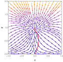
(a) Sugra with $\chi=\gamma=1$ and $\xi=\frac{1}{10}$.

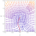
(b) Barreriro-Copeland-Nunes with $l=6$, $m=\frac{1}{2}$ and $\xi=\frac{1}{2}$.

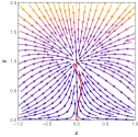
(c) Albrecht-Skordis with $A=B=\mu=\frac{1}{6}$ and $\xi=\frac{1}{10}$.

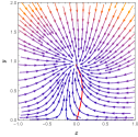
(d) Ureña-López-Matos with $n=-\frac{1}{2}$, $\zeta=\frac{1}{2}$ and $\xi=\frac{1}{2}$.

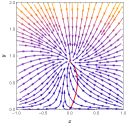
(e) Inverse exponential with $\xi=\frac{1}{6}$.

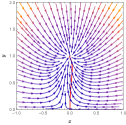
(f) Chang-Scherrer with $\tau=1$ and $\xi=1$.

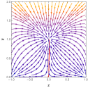
(g) Exponential with $\beta=10^{-1}$ and $\xi=\frac{1}{2}$.

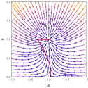
(h) Inverse hyperbolic cosine with $\alpha=2$ and $\xi=\frac{1}{6}$.

Figure 7: Phase-space trajectories on the $x-y$ plane for non-minimally coupled standard scalar field models. The coupling constant and initial conditions are also valid for the alternative scalar field description. Red lines indicate the solutions of the dynamical systems.

References

- [1] S. Perlmutter et al. Measurements of and from 42 High Redshift Supernovae. Astrophys. J., 517:565–586, 1999.
- [2] S. Perlmutter et al. Discovery of a supernova explosion at half the age of the Universe and its cosmological implications. Nature, 391:51–54, 1998.
- [3] Adam G. Riess et al. Observational evidence from supernovae for an accelerating universe and a cosmological constant. Astron. J., 116:1009–1038, 1998.
- [4] P. J. E. Peebles and Bharat Ratra. The Cosmological Constant and Dark Energy. Rev. Mod. Phys., 75:559–606, 2003.
- [5] N. Aghanim et al. Planck 2018 results. V. CMB power spectra and likelihoods. Astron. Astrophys., 641:A5, 2020.
- [6] Y. Akrami et al. Planck 2018 results. VII. Isotropy and Statistics of the CMB. Astron. Astrophys., 641:A7, 2020.
- [7] N. Aghanim et al. Planck 2018 results. I. Overview and the cosmological legacy of Planck. Astron. Astrophys., 641:A1, 2020.
- [8] N. Aghanim et al. Planck 2018 results. VI. Cosmological parameters. Astron. Astrophys., 641:A6, 2020. [Erratum: Astron.Astrophys. 652, C4 (2021)].
- [9] Youri Carloni, Orlando Luongo, and Marco Muccino. Does dark energy really revive using DESI 2024 data? 4 2024.
- [10] A. G. Adame et al. DESI 2024 VI: Cosmological Constraints from the Measurements of Baryon Acoustic Oscillations. 4 2024.
- [11] Gong-Bo Zhao et al. Dynamical dark energy in light of the latest observations. Nature Astron., 1(9):627–632, 2017.
- [12] Marco Muccino, Luca Izzo, Orlando Luongo, Kuantay Boshkayev, Lorenzo Amati, Massimo Della Valle, Giovanni Battista Pisani, and Elena Zaninoni. Tracing dark energy history with gamma ray bursts. Astrophys. J., 908(2):181, 2021.
- [13] Tengpeng Xu, Yun Chen, Lixin Xu, and Shuo Cao. Comparing the scalar-field dark energy models with recent observations. Phys. Dark Univ., 36:101023, 2022.
- [14] Edmund J. Copeland, M. Sami, and Shinji Tsujikawa. Dynamics of dark energy. Int. J. Mod. Phys. D, 15:1753–1936, 2006.
- [15] Olga Avsajanishvili, Gennady Y. Chitov, Tina Kahniashvili, Sayan Mandal, and Lado Samushia. Observational Constraints on Dynamical Dark Energy Models. Universe, 10(3):122, 2024.
- [16] Peter K. S. Dunsby, Orlando Luongo, and Lorenzo Reverberi. Dark Energy and Dark Matter from an additional adiabatic fluid. Phys. Rev. D, 94(8):083525, 2016.
- [17] Eleonora Di Valentino, Olga Mena, Supriya Pan, Luca Visinelli, Weiqiang Yang, Alessandro Melchiorri, David F. Mota, Adam G. Riess, and Joseph Silk. In the realm of the Hubble tension—a review of solutions. Class. Quant. Grav., 38(15):153001, 2021.
- [18] Jose Luis Bernal, Licia Verde, and Adam G. Riess. The trouble with . JCAP, 10:019, 2016.
- [19] Sunny Vagnozzi. New physics in light of the tension: An alternative view. Phys. Rev. D, 102(2):023518, 2020.
- [20] Catherine Heymans et al. KiDS-1000 Cosmology: Multi-probe weak gravitational lensing and spectroscopic galaxy clustering constraints. Astron. Astrophys., 646:A140, 2021.
- [21] Marika Asgari et al. KiDS-1000 Cosmology: Cosmic shear constraints and comparison between two point statistics. Astron. Astrophys., 645:A104, 2021.
- [22] H. Hildebrandt et al. KiDS+VIKING-450: Cosmic shear tomography with optical and infrared data. Astron. Astrophys., 633:A69, 2020.
- [23] Eleonora Di Valentino, Céline Bøehm, Eric Hivon, and François R. Bouchet. Reducing the and tensions with Dark Matter-neutrino interactions. Phys. Rev. D, 97(4):043513, 2018.
- [24] A. D. Sakharov. Vacuum quantum fluctuations in curved space and the theory of gravitation. Dokl. Akad. Nauk Ser. Fiz., 177:70–71, 1967.
- [25] Steven Weinberg. The Cosmological constant problems. In 4th International Symposium on Sources and Detection of Dark Matter in the Universe (DM 2000), pages 18–26, 2 2000.
- [26] Sean M. Carroll. The Cosmological constant. Living Rev. Rel., 4:1, 2001.
- [27] A. D. Dolgov. The Problem of vacuum energy and cosmology. In 4th Paris Cosmology Colloquium, pages 161–175, 6 1997.
- [28] Varun Sahni and Alexei A. Starobinsky. The Case for a positive cosmological Lambda term. Int. J. Mod. Phys. D, 9:373–444, 2000.
- [29] N. Straumann. The Mystery of the cosmic vacuum energy density and the accelerated expansion of the universe. Eur. J. Phys., 20:419–427, 1999.
- [30] S. E. Rugh and H. Zinkernagel. The Quantum vacuum and the cosmological constant problem. Stud. Hist. Phil. Sci. B, 33:663–705, 2002.
- [31] T. Padmanabhan. Cosmological constant: The Weight of the vacuum. Phys. Rept., 380:235–320, 2003.
- [32] Jun’ichi Yokoyama. Issues on the cosmological constant. In 12th Workshop on General Relativity and Gravitation, 5 2003.
- [33] Jerome Martin. Everything You Always Wanted To Know About The Cosmological Constant Problem (But Were Afraid To Ask). Comptes Rendus Physique, 13:566–665, 2012.
- [34] Vivian Poulin, Tristan L. Smith, Tanvi Karwal, and Marc Kamionkowski. Early Dark Energy Can Resolve The Hubble Tension. Phys. Rev. Lett., 122(22):221301, 2019.
- [35] Tanvi Karwal and Marc Kamionkowski. Dark energy at early times, the Hubble parameter, and the string axiverse. Phys. Rev. D, 94(10):103523, 2016.
- [36] Sk. Sohail, Sonej Alam, Shiriny Akthar, and Md. Wali Hossain. Quintessential early dark energy. 8 2024.
- [37] Dragan Huterer, Glenn D. Starkman, and Mark Trodden. Is the universe inflating? Dark energy and the future of the universe. Phys. Rev. D, 66:043511, 2002.
- [38] Jun’ichi Yokoyama. Vacuum selection by inflation as the origin of the dark energy. Int. J. Mod. Phys. D, 11:1603–1608, 2002.
- [39] William Giarè. Inflation, the Hubble tension, and early dark energy: An alternative overview. Phys. Rev. D, 109(12):123545, 2024.
- [40] P. Brax and P. Vanhove. effectively from Inflation to Dark Energy. 5 2024.
- [41] Leandros Perivolaropoulos and Foteini Skara. Challenges for CDM: An update. New Astron. Rev., 95:101659, 2022.
- [42] Philip Bull et al. Beyond CDM: Problems, solutions, and the road ahead. Phys. Dark Univ., 12:56–99, 2016.
- [43] Gabriel P. Lynch, Lloyd Knox, and Jens Chluba. DESI and the Hubble tension in light of modified recombination. 6 2024.
- [44] Sihem zabat, Youcef Kehal, and Khireddine Nouicer. Alleviating the and tensions in the interacting cubic covariant Galileon model. 5 2024.
- [45] Hao Wang and Yun-Song Piao. Dark energy in light of recent DESI BAO and Hubble tension. 4 2024.
- [46] Itamar J. Allali, Alessio Notari, and Fabrizio Rompineve. Dark Radiation with Baryon Acoustic Oscillations from DESI 2024 and the tension. 4 2024.
- [47] Timothy Clifton and Neil Hyatt. A Radical Solution to the Hubble Tension Problem. 4 2024.
- [48] Pedro Carrilho, Chiara Moretti, and Maria Tsedrik. Probing solutions to the tension with galaxy clustering. In Rencontres de Blois 2023, 10 2023.
- [49] Meng-Zhen Lyu, Balakrishna S. Haridasu, Matteo Viel, and Jun-Qing Xia. Reconstruction with Type Ia Supernovae, Baryon Acoustic Oscillation and Gravitational Lensing Time-Delay. Astrophys. J., 900(2):160, 2020.
- [50] William J. Wolf and Pedro G. Ferreira. Underdetermination of dark energy. Phys. Rev. D, 108(10):103519, 2023.
- [51] Marek Szydlowski and Orest Hrycyna. Scalar field cosmology in the energy phase-space – unified description of dynamics. JCAP, 01:039, 2009.
- [52] M. R. Setare and Elias C. Vagenas. Non-minimal coupling of the phantom field and cosmic acceleration. Astrophys. Space Sci., 330:145–150, 2010.
- [53] Orest Hrycyna. What ? Cosmological constraints on the non-minimal coupling constant. Phys. Lett. B, 768:218–227, 2017.
- [54] Orlando Luongo and Tommaso Mengoni. Generalized K-essence inflation in Jordan and Einstein frames. Class. Quant. Grav., 41(10):105006, 2024.
- [55] David I. Kaiser. Nonminimal Couplings in the Early Universe: Multifield Models of Inflation and the Latest Observations. Fundam. Theor. Phys., 183:41–57, 2016.
- [56] Yohei Ema, Mindaugas Karciauskas, Oleg Lebedev, and Marco Zatta. Early Universe Higgs dynamics in the presence of the Higgs-inflaton and non-minimal Higgs-gravity couplings. JCAP, 06:054, 2017.
- [57] Sebastian Bahamonde, Christian G. Böhmer, Sante Carloni, Edmund J. Copeland, Wei Fang, and Nicola Tamanini. Dynamical systems applied to cosmology: dark energy and modified gravity. Phys. Rept., 775-777:1–122, 2018.
- [58] Eleonora Di Valentino, Alessandro Melchiorri, Olga Mena, and Sunny Vagnozzi. Nonminimal dark sector physics and cosmological tensions. Phys. Rev. D, 101(6):063502, 2020.
- [59] Grigoris Panotopoulos. Nonminimal GUT inflation after Planck results. Phys. Rev. D, 89(4):047301, 2014.
- [60] Kourosh Nozariand and Narges Rashidi. Testing an Inflation Model with Nonminimal Derivative Coupling in the Light of PLANCK 2015 Data. Adv. High Energy Phys., 2016:1252689, 2016.
- [61] Mehdi Eshaghi, Moslem Zarei, Nematollah Riazi, and Ahmad Kiasatpour. A Non-minimally Coupled Potential for Inflation and Dark Energy after Planck 2015: A Comprehensive Study. JCAP, 11:037, 2015.
- [62] Sergio del Campo, Carlos Gonzalez, and Ramón Herrera. Power law inflation with a non-minimally coupled scalar field in light of Planck 2015 data: the exact versus slow roll results. Astrophys. Space Sci., 358(2):31, 2015.
- [63] Nilay Bostan and Shouvik Roy Choudhury. First constraints on non-minimally coupled Natural and Coleman-Weinberg inflation and massive neutrino self-interactions with Planck+BICEP/Keck. JCAP, 07:032, 2024.
- [64] Vahid Kamali. Non-minimal Higgs inflation in the context of warm scenario in the light of Planck data. Eur. Phys. J. C, 78(11):975, 2018.
- [65] Xavier Calmet and Iberê Kuntz. Higgs Starobinsky Inflation. Eur. Phys. J. C, 76(5):289, 2016.
- [66] Andreas Mantziris, Tommi Markkanen, and Arttu Rajantie. The effective Higgs potential and vacuum decay in Starobinsky inflation. JCAP, 10:073, 2022.
- [67] Swagat S. Mishra, Daniel Müller, and Aleksey V. Toporensky. Generality of Starobinsky and Higgs inflation in the Jordan frame. Phys. Rev. D, 102(6):063523, 2020.
- [68] Miguel Barroso Varela and Orfeu Bertolami. Hubble tension in a nonminimally coupled curvature-matter gravity model. JCAP, 06:025, 2024.
- [69] Salvatore Capozziello, Rocco D’Agostino, and Orlando Luongo. Thermodynamic parametrization of dark energy. Phys. Dark Univ., 36:101045, 2022.
- [70] Glennys R. Farrar and P. James E. Peebles. Interacting dark matter and dark energy. Astrophys. J., 604:1–11, 2004.
- [71] B. Wang, E. Abdalla, F. Atrio-Barandela, and D. Pavon. Dark Matter and Dark Energy Interactions: Theoretical Challenges, Cosmological Implications and Observational Signatures. Rept. Prog. Phys., 79(9):096901, 2016.
- [72] Jose Beltrán Jiménez, Lavinia Heisenberg, and Tomi S. Koivisto. The Geometrical Trinity of Gravity. Universe, 5(7):173, 2019.
- [73] Orlando Luongo. Revising the cosmological constant problem through a fluid different from the quintessence. Phys. Sci. Tech., 10(3-4):17–27, 2023.
- [74] Changjun Gao, Martin Kunz, Andrew R. Liddle, and David Parkinson. Unified dark energy and dark matter from a scalar field different from quintessence. Phys. Rev. D, 81:043520, 2010.
- [75] Orlando Luongo and Marco Muccino. Speeding up the universe using dust with pressure. Phys. Rev. D, 98(10):103520, 2018.
- [76] Rocco D’Agostino, Orlando Luongo, and Marco Muccino. Healing the cosmological constant problem during inflation through a unified quasi-quintessence matter field. Class. Quant. Grav., 39(19):195014, 2022.
- [77] Scott F. Daniel, Eric V. Linder, Tristan L. Smith, Robert R. Caldwell, Asantha Cooray, Alexie Leauthaud, and Lucas Lombriser. Testing General Relativity with Current Cosmological Data. Phys. Rev. D, 81:123508, 2010.
- [78] Paolo Creminelli, Guido D’Amico, Jorge Norena, Leonardo Senatore, and Filippo Vernizzi. Spherical collapse in quintessence models with zero speed of sound. JCAP, 03:027, 2010.
- [79] Stefano Camera, Carmelita Carbone, and Lauro Moscardini. Inclusive Constraints on Unified Dark Matter Models from Future Large-Scale Surveys. JCAP, 03:039, 2012.
- [80] Alessio Belfiglio, Roberto Giambò, and Orlando Luongo. Alleviating the cosmological constant problem from particle production. Class. Quant. Grav., 40(10):105004, 2023.
- [81] Alessio Belfiglio, Youri Carloni, and Orlando Luongo. Particle production from non-minimal coupling in a symmetry breaking potential transporting vacuum energy. Phys. Dark Univ., 44:101458, 2024.
- [82] Shin’ichi Nojiri and Sergei D. Odintsov. Introduction to modified gravity and gravitational alternative for dark energy. eConf, C0602061:06, 2006.
- [83] Thomas P. Sotiriou and Valerio Faraoni. f(R) Theories Of Gravity. Rev. Mod. Phys., 82:451–497, 2010.
- [84] Antonio De Felice and Shinji Tsujikawa. f(R) theories. Living Rev. Rel., 13:3, 2010.
- [85] Chao-Qiang Geng, Chung-Chi Lee, Emmanuel N. Saridakis, and Yi-Peng Wu. “Teleparallel” dark energy. Phys. Lett. B, 704:384–387, 2011.
- [86] Jose Beltrán Jiménez, Lavinia Heisenberg, and Tomi Koivisto. Coincident General Relativity. Phys. Rev. D, 98(4):044048, 2018.
- [87] Lavinia Heisenberg, Manuel Hohmann, and Simon Kuhn. Cosmological teleparallel perturbations. JCAP, 03:063, 2024.
- [88] Sebastian Bahamonde, Konstantinos F. Dialektopoulos, Celia Escamilla-Rivera, Gabriel Farrugia, Viktor Gakis, Martin Hendry, Manuel Hohmann, Jackson Levi Said, Jurgen Mifsud, and Eleonora Di Valentino. Teleparallel gravity: from theory to cosmology. Rept. Prog. Phys., 86(2):026901, 2023.
- [89] Timothy Clifton, Pedro G. Ferreira, Antonio Padilla, and Constantinos Skordis. Modified Gravity and Cosmology. Phys. Rept., 513:1–189, 2012.
- [90] Behrouz Mirza and Fatemeh Oboudiat. Mimetic f(T) Teleparallel gravity and cosmology. Gen. Rel. Grav., 51(7):96, 2019.
- [91] Je-An Gu, Chung-Chi Lee, and Chao-Qiang Geng. Teleparallel Dark Energy with Purely Non-minimal Coupling to Gravity. Phys. Lett. B, 718:722–726, 2013.
- [92] Youri Carloni and Orlando Luongo. Phase-space analysis in non-minimal symmetric-teleparallel dark energy. Eur. Phys. J. C, 84(5):519, 2024.
- [93] Sayantan Ghosh, Raja Solanki, and P. K. Sahoo. Dynamical system analysis of scalar field cosmology in coincident f(Q) gravity. Phys. Scripta, 99(5):055021, 2024.
- [94] Jianbo Lu, Xin Zhao, and Guoying Chee. Cosmology in symmetric teleparallel gravity and its dynamical system. Eur. Phys. J. C, 79(6):530, 2019.
- [95] M. Koussour, N. Myrzakulov, Alnadhief H. A. Alfedeel, E. I. Hassan, D. Sofuoğlu, and Safa M. Mirgani. Square-root parametrization of dark energy in f(Q) cosmology. Commun. Theor. Phys., 75(12):125403, 2023.
- [96] Rocco D’Agostino and Orlando Luongo. Growth of matter perturbations in nonminimal teleparallel dark energy. Phys. Rev. D, 98(12):124013, 2018.
- [97] Salvatore Capozziello, Alessio Lapponi, Orlando Luongo, and Stefano Mancini. Preserving quantum information in cosmology. 6 2024.
- [98] Philippe Brax and Jerome Martin. The Robustness of quintessence. Phys. Rev. D, 61:103502, 2000.
- [99] Philippe Brax and Jerome Martin. Quintessence and supergravity. Phys. Lett. B, 468:40–45, 1999.
- [100] R. R. Caldwell and Eric V. Linder. The Limits of quintessence. Phys. Rev. Lett., 95:141301, 2005.
- [101] T. Barreiro, Edmund J. Copeland, and N. J. Nunes. Quintessence arising from exponential potentials. Phys. Rev. D, 61:127301, 2000.
- [102] Andreas Albrecht and Constantinos Skordis. Phenomenology of a realistic accelerating universe using only Planck scale physics. Phys. Rev. Lett., 84:2076–2079, 2000.
- [103] S. C. C. Ng, N. J. Nunes, and Francesca Rosati. Applications of scalar attractor solutions to cosmology. Phys. Rev. D, 64:083510, 2001.
- [104] L. Arturo Urena-Lopez and Tonatiuh Matos. A New cosmological tracker solution for quintessence. Phys. Rev. D, 62:081302, 2000.
- [105] Hui-Yiing Chang and Robert J. Scherrer. Reviving Quintessence with an Exponential Potential. 8 2016.
- [106] Robert J. Scherrer and A. A. Sen. Phantom Dark Energy Models with a Nearly Flat Potential. Phys. Rev. D, 78:067303, 2008.
- [107] M. Sami and Alexey Toporensky. Phantom field and the fate of universe. Mod. Phys. Lett. A, 19:1509, 2004.
- [108] Parampreet Singh, M. Sami, and Naresh Dadhich. Cosmological dynamics of phantom field. Phys. Rev. D, 68:023522, 2003.
- [109] Abdulla Al Mamon and Sudipta Das. A parametric reconstruction of the deceleration parameter. Eur. Phys. J. C, 77(7):495, 2017.
- [110] Matt Visser. Cosmography: Cosmology without the Einstein equations. Gen. Rel. Grav., 37:1541–1548, 2005.
- [111] Salvatore Capozziello, Peter K. S. Dunsby, and Orlando Luongo. Model-independent reconstruction of cosmological accelerated–decelerated phase. Mon. Not. Roy. Astron. Soc., 509(4):5399–5415, 2021.
- [112] Orlando Luongo and Marco Muccino. Kinematic constraints beyond using calibrated GRB correlations. Astron. Astrophys., 641:A174, 2020.
- [113] Orlando Luongo and Marco Muccino. Model independent cosmographic constraints from DESI 2024. 4 2024.
- [114] Andrei D. Linde. Inflationary Cosmology. Lect. Notes Phys., 738:1–54, 2008.
- [115] Marek Szydlowski, Orest Hrycyna, and Aleksander Stachowski. Scalar field cosmology - geometry of dynamics. Int. J. Geom. Meth. Mod. Phys., 11:1460012, 2014.
- [116] Christian G. Boehmer, Nyein Chan, and Ruth Lazkoz. Dynamics of dark energy models and centre manifolds. Phys. Lett. B, 714:11–17, 2012.
- [117] Shuang-Yong Zhou. A New Approach to Quintessence and Solution of Multiple Attractors. Phys. Lett. B, 660:7–12, 2008.
- [118] J. S. Farnes. A unifying theory of dark energy and dark matter: Negative masses and matter creation within a modified CDM framework. Astron. Astrophys., 620:A92, 2018.
- [119] Luca Visinelli, Sunny Vagnozzi, and Ulf Danielsson. Revisiting a negative cosmological constant from low-redshift data. Symmetry, 11(8):1035, 2019.
- [120] Nicola Menci, Shahnawaz A. Adil, Upala Mukhopadhyay, Anjan A. Sen, and Sunny Vagnozzi. Negative cosmological constant in the dark energy sector: tests from JWST photometric and spectroscopic observations of high-redshift galaxies. JCAP, 07:072, 2024.
- [121] Chen Xu, Emmanuel N. Saridakis, and Genly Leon. Phase-Space analysis of Teleparallel Dark Energy. JCAP, 07:005, 2012.
- [122] Sudipta Das, Manisha Banerjee, and Nandan Roy. Dynamical System Analysis for Steep Potentials. JCAP, 08:024, 2019.