AlphaPruning: Using Heavy-Tailed Self Regularization Theory for Improved Layer-wise Pruning of Large Language Models

Abstract

Recent work on pruning large language models (LLMs) has shown that one can eliminate a large number of parameters without compromising performance, making pruning a promising strategy to reduce LLM model size. Existing LLM pruning strategies typically assign uniform pruning ratios across layers, limiting overall pruning ability; and recent work on layerwise pruning of LLMs is often based on heuristics that can easily lead to suboptimal performance. In this paper, we leverage Heavy-Tailed Self-Regularization (HT-SR) Theory, in particular the shape of empirical spectral densities (ESDs) of weight matrices, to design improved layerwise pruning ratios for LLMs. Our analysis reveals a wide variability in how well-trained, and thus relatedly how prunable, different layers of an LLM are. Based on this, we propose AlphaPruning, which uses shape metrics to allocate layerwise sparsity ratios in a more theoretically-principled manner. AlphaPruning can be used in conjunction with multiple existing LLM pruning methods. Our empirical results show that AlphaPruning prunes LLaMA-7B to 80% sparsity while maintaining reasonable perplexity, marking a first in the literature on LLMs. We have open-sourced our code.

1 Introduction

Recent work on pruning large language models (LLMs) Jaiswal et al. (2023); Frantar and Alistarh (2023a); Sun et al. (2023) has shown the ability to reduce the number of parameters significantly, without compromising performance, resulting in notable savings in memory footprint, computing time, and energy consumption. Unlike pre-LLM pruning methods Sanh et al. (2020); Kurtic et al. (2022), existing LLM pruning approaches typically allocate the “sparsity budget” (i.e., the number of pruned parameters or pruning ratios) uniformly across layers, making it difficult to increase sparsity to very high levels. Relatively little effort has been put into developing theoretically-principled ways to compute layerwise pruning ratios. For example, the Outlier Weighed Layerwise sparsity (OWL) method Yin et al. (2023) uses a nonuniform layerwise sparsity based on the distribution of outlier activations. However, OWL relies on heuristics related to the presence of outliers Kovaleva et al. (2021); Puccetti et al. (2022); Dettmers et al. (2022). This can lead to suboptimal performance in the absence of outliers, and this can make it difficult to achieve very aggressive levels of sparsity. For example, Yin et al. (2023) shows that pruning LLMs to 80% sparsity often significantly degrades the prediction performance of LLMs.

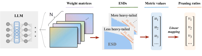
Figure 1: The pipeline diagram of AlphaPruning. Our post-training layer-wise pruning method involves the following steps: (i) Performing ESD analysis on all weight matrices of a base LLM and (ii) employing PL fitting to derive the layer-wise metric values (that measures the HT exponent). Then, (iii) using the layer-wise metric values, we assign layer-wise pruning ratios to each layer through a linear assignment function.

In developing a principled approach to allocate sparsity budgets across layers, we draw inspiration from Heavy-Tailed Self-Regularization (HT-SR) Theory Martin et al. (2021); Martin and Mahoney (2021a, b, 2019, 2017, 2020); Yang et al. (2023); Zhou et al. (2023). HT-SR theory analyzes the weight matrices of models to derive quantities (related to the shape of the weight matrix eigenspectrum), which help characterize model capacity and quality. Applications of HT-SR to model selection Martin and Mahoney (2019, 2020, 2021a); Martin et al. (2021); Yang et al. (2023) and layer-wise adaptive training Zhou et al. (2023) demonstrate the effectiveness of the theory in estimating model and layer quality. Furthermore, in the context of pruning memory/computation-efficient LLMs, using this kind of low-cost weight analysis is advantageous because it requires no data or gradient backpropagation.

Our study consists of two main parts. In the first part, we evaluate the effectiveness of various weight matrix-based metrics for allocating layer-wise sparsity. Our primary finding indicates that shape metrics generally outperform scale metrics in determining layer importance for pruning. Shape metrics capture the shape properties of the empirical spectral densities (ESDs) of layer weight matrices, whereas scale metrics, like matrix norms, reflect the size or scale of ESDs. This offers a novel perspective since shape metrics are less frequently used in the literature than scale metrics, which have been used to create regularizers Yoshida and Miyato (2017) and inform pruning Han et al. (2015).

In the second part of the paper, we introduce a theoretically principled layer-wise sparsity allocation method, AlphaPruning, based on metrics that quantify a unique heavy-tailed (HTed) shape of ESDs. According to HT-SR theory, well-trained models display strong correlations among the weight matrix elements, leading to HT structures in layer weight matrices’ ESDs Martin and Mahoney (2019, 2020, 2021a). Moreover, layers with more pronounced HT properties are typically better trained than others. We quantify the HT properties by fitting a power law (PL) distribution Alstott et al. (2014); Clauset et al. (2009) to ESD and using the PL exponent as the HT metric PL_Alpha_Hill. The principle of AlphaPruning is to allocate less sparsity to more well-trained (more HTed) layers, as indicated by lower PL_Alpha_Hill values, thereby preserving their quality during pruning. Figure 1 illustrates the pipeline of AlphaPruning.

We conducted a comprehensive empirical evaluation to assess the generalizability of AlphaPruning in LLM pruning. This evaluation involved comparisons with various baseline methods, integration with existing techniques, and testing across different architectures. We also conducted sanity checks to ensure that AlphaPruning indeed reduces the variation of PL_Alpha_Hill values across layers. Our key contributions are summarized below.

• This paper is the first to study principled layer-wise sparsity allocation from the HT-SR perspective. We systematically evaluate multiple weight matrix-based metrics to compute sparsity based on their effectiveness in estimating layer quality, discovering an interesting finding: shape metrics outperform scale metrics in allocating sparsity, despite the latter being more commonly used.

• We introduce a novel sparsity allocation method, AlphaPruning, inspired by HT-SR theory, which demonstrates superior performance in LLM pruning. This method assigns sparsities based on the heavy-tailed shape of ESDs in layer weight matrices, a previously unexplored concept. Our empirical evaluations span a range of LLM architectures, including the LLaMA V1-3 families Touvron et al. (2023a, b), OPT families Zhang et al. (2023), Vicuna-7B Zheng et al. (2024), and Mistral-7B Jiang et al. (2023). The results show that AlphaPruning outperforms OWL Yin et al. (2023), the current SOTA non-uniform sparsity allocation method for LLMs, reducing perplexity by 304.31 and achieving an average accuracy gain of 4.6% over 7 zero-shot tasks at 80% sparsity, while providing a 3.06$\times$ end-to-end speedup on CPUs for LLaMA-7B on the DeepSparse NeuralMagic (2021) inference engine. AlphaPruning also outperforms six layer-wise allocation methods, including global thresholding Frankle and Carbin (2018), ER Mocanu et al. (2018), ER-Plus Liu et al. (2022a), LAMP Lee et al. (2020), rank selection Kuzmin et al. (2019); El Halabi et al. (2022), and layer-wise error thresholding Ye et al. (2020); Zhuang et al. (2018).

• AlphaPruning provides layer-wise budget allocation (e.g., sparsity), demonstrating remarkable generalizability and can be integrated with multiple LLM compression techniques to enhance performance. This includes unstructured pruning (Wanda Sun et al. (2023), SparseGPT Frantar and Alistarh (2023b)), with or without fine-tuning Hu et al. (2021), semi-structured (DominoSearch Sun et al. (2021)), structured pruning (LLMPruner Ma et al. (2023), OSSCAR Meng et al. (2024)), mixed-precision quantization Tang et al. (2022). Additionally, we have extended this method to large Computer Vision (CV) architectures, such as Vision Transformers (ViT) Dosovitskiy et al. (2020), and ConvNext Liu et al. (2022b). In this case, OWL significantly underperforms AlphaPruning due to the lack of outlier features. This indicates HT metrics are more general than outlier metrics.

• AlphaPruning is theoretically driven, and its improvements can be interpreted by HT-SR metrics. We demonstrate that model performance correlates with model-wise and layer-wise changes in PL_Alpha_Hill before and after pruning. Furthermore, compared to baseline pruning methods, AlphaPruning not only improves model performance but also achieves a lower mean of layer-wise PL_Alpha_Hill. HT-SR theory suggests that AlphaPruning preserves the quality of model layers “on average”, minimizing the damage caused by pruning.

2 Related work

Pruning.

Removing weights or connections in a trained neural network (NN) to generate an efficient, compressed model has a long history LeCun et al. (1990); Mozer and Smolensky (1988); Janowsky (1989); Mocanu et al. (2018). Modern NNs are frequently over-parameterized Wang and Tu (2020); Bhojanapalli et al. (2021), and thus removing redundancies improves computation and memory efficiency. A common approach is weight-magnitude-based pruning Han et al. (2015), which zeros out connections with weights smaller than a specified threshold. However, when it comes to pruning LLMs Brown et al. (2020); Touvron et al. (2023a), progress has been limited. Conventional pruning typically requires a round of retraining to restore performance Blalock et al. (2020), which can be challenging for LLMs. To address the difficulty in retraining, researchers have developed specially tailored pruning algorithms for LLMs. For example,  Ma et al. (2023) explored sparse structured LLMs, using Taylor pruning to remove entire weight rows, followed by LoRA fine-tuning. More recent research has shifted towards unstructured pruning without the need for fine-tuning, showing substantial advancements. In particular, SparseGPT Frantar and Alistarh (2023b) uses the Hessian inverse for pruning and subsequent weight updates to reduce the reconstruction error of dense and sparse weights, while Wanda Sun et al. (2023) uses a criterion that incorporates weight magnitudes and input activations, in order to preserve outlier features Kovaleva et al. (2021); Puccetti et al. (2022); Dettmers et al. (2022). Our work allocates parameters in a more theoretically-principled manner, enabling pruning LLMs to higher sparsity levels.

Layerwise sparsity budgets.

Although layerwise sparsity has been widely studied in pre-LLM pruning (Mocanu et al., 2018; Evci et al., 2020; Liu et al., 2022a; Gale et al., 2019; Lee et al., 2020), relatively little attention has been devoted to determining the pruning ratios for each layer in LLMs. (Interestingly, this layer-wise approach has been applied to model quantization Kim et al. (2023); Shen et al. (2020); Dong et al. (2019).) Frantar and Alistarh (2023b) and Sun et al. (2023) apply a uniform pruning ratio across all layers, and Yin et al. (2023) computes the sparsity budgets using the outlier ratio observed within each layer’s token feature distribution. Existing work on sparsity budgets has generally used heuristics, such as different forms of size or scale metrics (such as norm-based metrics), to determine sparsity budgets per layer. For instance, ABCPruner Lin et al. (2020) reduces the number of combinations of layer sparsities to search over, but it still requires training to determine the empirical validity of its suggested layer sparsities. Lee et al. (2020) modifies Magnitude-based pruning by rescaling the importance scores in a layer by a factor dependent on the magnitude of surviving connections in that layer. However, these methods are suboptimal in allocating layerwise sparsities for pruning LLMs. Recently, Outlier Weighed Layerwise sparsity (OWL) Yin et al. (2023) designs a nonuniform layerwise sparsity based on the distribution of outlier activations in LLMs. However, OWL heuristically relies on the emergence of outliers, and this can lead to suboptimal performance when outliers are absent from models. Our work uses HT-SR shape metrics such as PL_Alpha_Hill to predict layer importance, and it allocates parameters in a more theoretically principled manner, allowing pruning LLMs to higher sparsity levels than has ever been achieved before.

3 Background and Setup

3.1 Notation

Consider a NN with $L$ layers, $\mathbf{W}_{i}$ is one of the weight matrices extracted from the $i$-th layer with shape $m\times n$ ($m\geq n$). We note that the “layer” used in this work refers to the transformer block (layer), and each block contains multiple weight matrices, such as the attention layer weight matrix, and projection layer weight matrix. The correlation matrix $\mathbf{X}_{i}=\mathbf{W}_{i}^{\top}\mathbf{W}_{i}$ is an $n\times n$ symmetric matrix, and the ESD of $\mathbf{X}_{i}$ is formulated as

$$\mu_{\mathbf{X}_{i}}:=\frac{1}{n}\sum_{j=1}^{n}\delta_{\lambda_{j}\left(\mathbf{X}_{i}\right)}$$ (1)

where $\lambda_{1}\left(\mathbf{X}_{i}\right)\leq\ldots\leq\lambda_{n}\left(\mathbf{X}_{i}\right)$ are the eigenvalues of $\mathbf{X}_{i}$ and $\delta$ is the Dirac delta function. The ESD is a probability measure, which can be viewed as a distribution of the eigenvalues of $\mathbf{X}_{i}$.

3.2 HT-SR theory and metrics

Here, we provide a brief overview of HT-SR theory. HR-SR theory originated as a semi-empirical theory, with early seminal work Martin and Mahoney (2019); Martin et al. (2021) examining the empirical spectral density (ESD) of weight matrices, specifically the eigenspectrum of the correlation matrix $\mathbf{X}_{i}=\mathbf{W}_{i}^{\top}\mathbf{W}_{i}$. This research found that the structures of the ESDs strongly correlate with training quality. These findings are rooted in statistical physics and Random Matrix Theory Couillet and Liao (2022), as detailed in Table 1 of Martin and Mahoney (2019). It is well-known Wang et al. (2024); Couillet and Liao (2022) that spikes in ESD represent “signals,” while the bulk represents noise, which follows the Marchenko-Pastur law. In the theoretical setting of Wang et al. (2024), the signal or the spike aligns with ground-truth features from the teacher model, and that corresponds to increased correlations in weight elements. Furthermore, Kothapalli et al. (2024) show that heavy tails in ESD originate from the interaction between spikes and bulk, which can be quantified precisely using recent advances in the free-probability theory Landau et al. (2023), and the interaction characterizes the “bulk-decay” phase in the five-plus-one phase model in Martin and Mahoney (2019), a critical phase between classical “bulk+spike” model and heavy-tail models.

To quantify the structure of ESDs, HT-SR theory provides several metrics, collectively known as HT-SR metrics. These metrics are typically categorized into two groups: scale metrics and shape metrics.

Scale metrics. Scale metrics refer to those obtained from measuring various norms of weight matrices. As demonstrated empirically in Yang et al. (2023), these metrics are often strongly correlated with the generalization gap (which is the gap between training and test performance), instead of the quality of the models. In this paper, we mainly study two scale metrics, Frobenius_Norm and Spectral_Norm. The Frobenius_Norm metric is calculated by the squared Frobenius norm of the weight matrix $\left\|\mathbf{W}\right\|^{2}_{F}$; and the Spectral_Norm metric can be calculated by the square of the spectral radius of the weight matrix $\left\|\mathbf{W}\right\|_{2}^{2}$.

Shape metrics. Drawing analytic methods from Random Matrix Theory, HT-SR work analyzes poorly trained and well-trained models and concludes that the performance of these models usually correlates with shapes emerging in their ESDs, such as “bulk+spike” shape or “heavy-tailed” shape. The metrics used to characterize these ESD shapes are called shape metrics, and we mainly studied four of them: PL_Alpha_Hill, Alpha_Hat, Stable_Rank, and Entropy. PL_Alpha_Hill is the main metric used in our method, and we define it in Section 4.2. The definitions of other shape metrics (including Alpha_Hat, Stable_Rank, Entropy) can be found in Appendix C.

4 Alpha-Pruning

In this section, we first outline the motivation behind AlphaPruning, followed by an introduction to the layer-wise importance metric, PL_Alpha_Hill, and the sparsity allocation function, as shown in Figure 1. Our empirical analysis reveals that shape metrics generally outperform scale metrics in guiding sparsity allocation with the same function. Notably, PL_Alpha_Hill, the shape metric used in AlphaPruning, achieves the best results in preliminary evaluations.

4.1 Rationale

HT-SR theory, introduced in Section 3.2, examines the ESD of weight matrices and finds a strong correlation between heavy-tailed structures in the ESD and training quality. It suggests that heavy-tailed structures emerge from feature learning, where useful correlations are extracted during optimization. Layers with more heavy-tailed ESDs tend to capture more signals, indicating better training quality. Inspired by these findings, we propose to assign sparsity based on the heavy-tailed properties of each layer’s ESD. Layers with more heavy-tailed ESDs, which contain more learned signals, are assigned lower sparsity, while layers with light-tailed ESDs are assigned higher sparsity. In practice, the heavy-tailed structure is measured by fitting a PL distribution to the ESD, and extracting the PL exponent $\alpha$ as the indicator. This is why our method is named AlphaPruning.

4.2 Estimating layer quality by HT metric

AlphaPruning relies on estimating the layer quality based on the HT characteristic of the layer ESDs, which is quantified by HT metric PL_Alpha_Hill. Given an ESD $\mu_{\mathbf{X}_{i}}$ of a weight matrix’s correlation matrix, we fit a PL density function $p(\lambda)$ on it, taking values within an interval ($\lambda_{\text{min}}$, $\lambda_{\text{max}}$), formally defined as:

$$p(\lambda)\propto\lambda^{-\alpha},\lambda_{\text{min}}<\lambda<\lambda_{\text{max}}.$$ (2)

The estimated exponent $\alpha$ is then used as a metric to characterize the HT extent of the ESD, with a lower value means more HTed. We estimate the PL coefficient using the Hill estimator Hill (1975); Xiao et al. (2023b); Zhou et al. (2023), and we refer to it as the PL_Alpha_Hill metric. The Hill estimator is defined as:

$$\texttt{PL\_Alpha\_Hill}=1+\frac{k}{(\sum_{i=1}^{k}\ln\frac{\lambda_{n-i+1}}{\lambda_{n-k}})},$$ (3)

where $\{\lambda_{i}\}_{i=1}^{n}$ is sorted in ascending order, and $k$ is a tunable parameter that adjusts the lower eigenvalue threshold $\lambda_{\text{min}}$ for (truncated) PL estimation. We adopt the Fix-finger method Yang et al. (2023) to select the $k$, which sets $k$ such that $\lambda_{\text{min}}$ aligns with the peak of the ESD. Note that PL_Alpha_Hill and other scale/shape metrics are calculated for each weight matrix individually.

4.3 Allocating sparsity based on the layer quality

AlphaPruning allocates sparsity for each layer (transformer block) by using a mapping function $\phi:\mathbb{R}^{L}\rightarrow\mathbb{R}^{L}$ to map a sequence of layer quality measures $\mathbf{q}=(q_{1},q_{2},..,q_{L})$ into corresponding sparsities $\phi(\mathbf{q})$.

$$\phi(\mathbf{q})_{i}=\eta\left[\frac{q_{i}-q_{\text{min}}}{q_{\text{max}}-q_{\text{min}}}(s_{2}-s_{1})+s_{1}\right].$$ (4)

Here, $\phi(\mathbf{q})_{i}$ represents the $i$-th element of the resulting vector $\phi(\mathbf{q})$, $q_{i}$ represents the $i$-th element of the input vector $\mathbf{q}$, and $q_{\text{min}}$, $q_{\text{max}}$ represent the minimum and maximum values of $\mathbf{q}$. The normalization factor $\eta$ adjusts the sparsity levels to achieve the target global sparsity $S$. Each layer’s sparsity is normalized within the interval $\left[\eta s_{1},\eta s_{2}\right]$. $\eta$ is calculated using the equation $\sum_{i=1}^{L}\phi(\mathbf{q})_{i}d_{i}=S\cdot\sum_{i=1}^{L}d_{i}$, in which $d_{i}$ is the number of parameters of $\mathbf{W}_{i}$. Both sides of the equation represent the total number of remaining parameters. The $(s_{1},s_{2})$ are tunable hyperparameters that adjust the non-uniformity of the sparsity distribution. We note that sparsity allocation is executed on a per-block basis, averaging the HT-SR metric across all matrices within a block to determine $q_{i}$. This design is supported by an ablation study, presented in Appendix E, which shows that it yields superior performance over a per-matrix allocation. Hyperparameter settings for all experiments are provided in Appendix F.

4.4 Shape vs. scale metrics for sparsity allocation

In this study, we evaluated various HT-SR metrics, as defined in Section 3.2, to assess their effectiveness in estimating layer quality $\mathbf{q}$ for computing layer-wise sparsity. Our preliminary experiments involved pruning the LLaMA-7B model to 70% sparsity and assessing its performance through WikiText perplexity and accuracy across seven zero-shot tasks, with results presented in Table 1. We applied each HT-SR metric in conjunction with three intra-layer pruning techniques (which only determine which matrix elements to prune), such as Magnitude, Wanda, and SparseGPT, to thoroughly evaluate their efficacy. Further experiments on Vision Transformers (ViT) are described in Appendix H.1. Across all tests, shape metrics consistently outperformed scale metrics in assigning layer-wise sparsities. This finding suggests that shape metrics are more robust and yield more reliable predictions of layer quality, which extends previous research Yang et al. (2023); Zhou et al. (2023); Martin et al. (2021) on estimating model quality. Notably, the shape metric PL_Alpha_Hill that focuses on estimating the HT shape, proved to be the most effective. Consequently, we have adopted PL_Alpha_Hill as the primary metric in our proposed method, AlphaPruning.

Metric used for	Perplexity on WikiText ($\downarrow$)			Average accuracy on 7 zero-shot tasks ($\uparrow$)
layerwise pruning ratios	Magnitude	Wanda	SparseGPT	Magnitude	Wanda	SparseGPT
Uniform	48419.13	85.77	26.30	32.30	36.73	41.52
Frobenius_Norm	30136.37	59.82	24.95	33.23	37.62	43.67
Spectral_Norm	48073.99	246.84	29.01	32.81	33.15	41.14
Entropy	3716.07	41.15	22.02	33.58	39.39	43.53
Stable_Rank	851.65	41.24	24.91	34.91	39.74	42.97
Alpha_Hat	1256.02	27.60	20.02	33.48	43.57	43.83
PL_Alpha_Hill	231.01	23.86	18.54	35.67	44.42	45.48

Table 1: Evaluating shape metrics versus scale metrics on allocating layerwise sparsities on LLMs. Shape metrics are obtained from the shapes of the ESDs. Scale metrics are norm-based metrics measuring the scale of weights matrices (which can also be obtained from the ESD). The results are conducted on LLaMA-7B at 70% sparsity. We show WikiText validation perplexity and average accuracy on seven different zero-shot tasks as evaluation metrics. We observe that shape metrics outperform scale metrics and PL_Alpha_Hill performs the best.

5 Empirical results

In this section, we evaluate the performance, generalizability, and interpretability of AlphaPruning. Section 5.1 outlines our experimental setup. In Section 5.2, we evaluate AlphaPruning’s performance by comparing it to the SOTA method OWL and five other baseline methods, and we analyze the efficiency of LLMs pruned by AlphaPruning using practical metrics such as FLOPs and latency. Section 5.3 evaluates the generalizability of AlphaPruning by integrating it with various LLM compression techniques including post-pruning fine-tuning, semi-structured pruning, structured pruning, and mixed-precision quantization. Additionally, we extend its application to CV tasks. Section 5.4 provides an analysis of the layer-wise sparsities and the PL_Alpha_Hill distribution to further elucidate the effectiveness and implications of AlphaPruning.

5.1 Experimental setup

Models and Evaluation. We evaluate AlphaPruning on the three most widely adopted LLM model families: LLaMA 7B/13B/30B/65B Touvron et al. (2023a), LLaMA-2 7B/13B/70B Touvron et al. (2023b), OPT 125M/350M/2.7B/6.7B, and other advanced LLMs: LLaMA-3-8B, Vicuna-7B, Mistral-7B. Our evaluation protocol aligns with established methodologies for LLM pruning Xiao et al. (2023a), including assessments of language modeling proficiency and zero-shot capabilities. Specifically, we evaluate the perplexity on the held-out WikiText Merity et al. (2016) validation set, and use seven tasks, including BoolQ Clark et al. (2019), RTE Wang et al. (2018), HellaSwag Zellers et al. (2019), WinoGrande Sakaguchi et al. (2021), ARC Easy and Challenge Clark et al. (2018) and OpenbookQA Mihaylov et al. (2018) for downstream zero-shot evaluation Gao et al. (2023).

Baselines.

We apply the layer-wise sparsities determined by AlphaPruning to three LLM pruning methods, including Magnitude Han et al. (2015), SparseGPT Frantar and Alistarh (2023b) and Wanda Sun et al. (2023). Magnitude-based pruning is a simple and strong baseline in which weights are discarded based on their magnitudes. Wanda and SparseGPT are two strong LLM pruning baselines due to their capability to sustain reasonable performance even at relatively high sparsity levels (around 50%). All these methods originally use uniform layerwise sparsity. We incorporate AlphaPruning directly into these baselines, and we demonstrate that this results in improved performance. Besides, we also compare AlphaPruning with OWL Yin et al. (2023), a recently proposed non-uniform LLM pruning method and six layer-wise pruning methods, including global thresholding Frankle and Carbin (2018), ER Mocanu et al. (2018), ER-Plus Liu et al. (2022a), LAMP Lee et al. (2020), rank selection Kuzmin et al. (2019); El Halabi et al. (2022), and layer-wise error thresholding Ye et al. (2020); Zhuang et al. (2018).

5.2 Main results

Language Modeling. In Table 2, we report the perplexity of the pruned LLaMA and LLaMA-2 models at 70% sparsity. We provide results for more sparsity levels in Figure 5.2 and Appendix G. AlphaPruning, as a general layerwise sparsity method, consistently demonstrates performance improvements when used in conjunction with various pruning methods. For example, in the case of LLaMA-7B with a sparsity of 70%, AlphaPruning produces sparse networks with a perplexity of 231.01, significantly outperforming the Magnitude-based pruning baseline of 48419.13. Notably, when applied to Wanda and SparseGPT, two robust LLM pruning methods, AlphaPruning still achieves substantial perplexity reductions, evidenced by a decrease of 61.91 for Wanda and 7.76 for SparseGPT, in the case of LLaMA-7B with a sparsity of 70%.

		LLaMA				LLaMA-2
Method	Layerwise sparsity	7B	13B	30B	65B	7B	13B	70B
Dense model	-	5.68	5.09	4.77	3.56	5.12	4.57	3.12
	Uniform	48419.13	84527.45	977.76	46.91	49911.45	214.04	1481.95
	OWL	19527.58	11464.69	242.57	15.16	59176.42	57.55	17.18
Magnitude	Ours	231.01	2029.20	62.39	16.01	8900.32	31.89	15.27
	Uniform	85.77	54.03	17.35	15.17	74.26	45.36	10.56
	OWL	24.57	17.17	10.75	8.61	30.38	20.70	8.52
Wanda	Ours	23.86	14.21	9.68	7.86	28.87	14.16	7.83
	Uniform	26.30	18.85	12.95	10.14	27.65	19.77	9.28
	OWL	19.49	14.55	10.28	8.28	20.40	15.27	7.65
SparseGPT	Ours	18.54	12.81	9.77	7.83	19.34	12.20	7.57

Table 2: WikiText validation perplexity for pruned LLaMA and LLaMA-2 models at 70% sparsity. Our method (AlphaPruning) is compared to uniform layerwise sparsity and OWL, each paired with magnitude-based pruning, Wanda, and SparseGPT. Lower perplexity indicates improved model performance.

Zero-shot tasks.

We conducted empirical evaluations to determine the zero-shot ability of pruned LLMs on diverse zero-shot downstream tasks with prompting. The results are shown in Table 3, where we show the mean zero-shot accuracy on 7 zero-shot tasks of pruned LLaMA and LLaMA-2 models at sparsity of 70%. AlphaPruning consistently improves accuracy across all settings. For example, AlphaPruning achieves an average accuracy gain of 8.79, 6.05, and 2.61 over 7 tasks and 7 models compared to Magnitude, Wanda and SparseGPT alone, respectively. These results highlight the promise of AlphaPruning for more challenging zero-shot downstream tasks.

		LLaMA				LLaMA-2
Method	Layerwise sparsity	7B	13B	30B	65B	7B	13B	70B
Dense model	-	60.08	62.59	65.47	67.05	59.71	63.05	67.06
	Uniform	32.30	34.95	32.39	45.04	33.38	33.56	43.65
	OWL	33.57	36.86	33.88	53.42	34.17	36.98	50.49
Magnitude	Ours	35.67	38.23	42.56	55.22	37.86	44.53	50.72
	Uniform	36.73	38.90	51.07	54.90	34.66	37.16	56.72
	OWL	43.41	45.91	52.38	57.34	40.46	45.04	57.19
Wanda	Ours	44.42	47.48	54.48	58.93	41.98	47.21	57.63
	Uniform	41.52	45.67	52.75	57.81	41.84	45.17	59.68
	OWL	44.65	47.61	53.16	58.25	44.96	47.94	59.20
SparseGPT	Ours	45.48	48.41	54.07	59.72	44.68	49.26	60.23

Table 3: Comparison of mean zero-shot accuracies (%) for pruned LLaMA and LLaMA-2 models at 70% sparsity. We evaluate our method (AlphaPruning) against uniform layerwise sparsity and OWL, each integrated with magnitude-based pruning, Wanda, and SparseGPT. Higher accuracy values indicate better zero-shot ability.

More baseline comparison.

For allocating layerwise sparsity ratios, we compare AlphaPruning with other allocation methods. The experiments involve pruning the LLaMA-7B model and LLaMA-13B to various sparsities. We use Wanda as the basic pruning method, with results presented in Figure 5.2 and Figure 5.2. Results indicate that AlphaPruning significantly outperforms all baseline methods in relatively high-sparsity regimes. For LLaMA-7B and LLaMA-13B pruned to 80% sparsity, AlphaPruning reduces perplexity by 304.31 and 200.54 compared to OWL, respectively. Achieving high levels of sparsity is crucial for unstructured sparsity to yield significant speedups on GPUs by leveraging existing sparse kernels. Sparse kernels such as Flash-LLM Xia et al. (2023) and Sputnik Gale et al. (2020) have shown that unstructured sparsity outperforms dense computation in terms of performance, but only when sparsity levels reach 60% and 71%, respectively. The importance of achieving high sparsity is further substantiated in the following section, which demonstrates that high sparsity levels facilitate significant end-to-end inference speedup. Additional comparisons with rank selection and layer-wise error thresholding, as well as results using SparseGPT as the pruning method and low sparsity results, can be found in Appendices G.

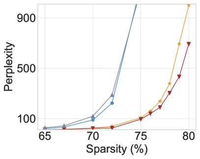
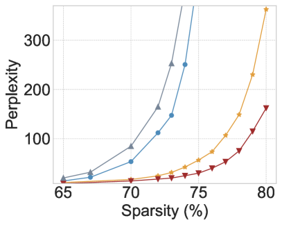
Figure 2: The WikiText validation perplexity for LLaMA-7B (left) and LLaMA-13B (right) pruned with different sparsities using Wanda.

Figure 3: Mean accuracy of 7 zero-shot tasks for LLaMA-7B pruned with different sparsities using Wanda.

Efficiency measure.

To verify the sparse LLM pruned by our method can indeed achieve speedups when deployed on the CPU, we provide new results in Table 4. We apply our method to Llama2-7B-Chat-hf, prune it to different sparsities, and then test its end-to-end decode latency using DeepSparse Kurtic et al. (2023) inference engine on an Intel Xeon Gold 6126 CPU with 24 cores. The results indicate that when the global sparsity reaches 80%, the speedup reaches 3.06$\times$.

Sparsity	Dense	10%	20%	30%	40%	50%	60%	70%	80%	90%
Latency (ms)	307.46	306.27	304.87	293.26	264.41	177.55	148.16	133.76	100.35	81.40
Throughput (tokens/sec)	3.25	3.26	3.28	3.41	3.78	5.63	6.74	7.47	9.96	12.28
Speedup	1.00x	1.00x	1.01x	1.05x	1.16x	1.73x	2.07x	2.30x	3.06x	3.78x

Table 4: End-to-end decode latency and speedup of AlphaPruning measured on the DeepSparse inference engine.

In Appendix H.2, we evaluate the pruned LLM by efficiency metrics other than sparsity, such as FLOPs, Compared with uniform sparsity ratios, our approach is able to achieve better performance-FLOPs trade-off. In Appendix H.3, we show that AlphaPruning can control the minimum layer sparsity without losing the performance advantage to meet the hardware requirements of a memory-limited device. In Appendix H.4, we report the runtime of AlphaPruning to show that the computational overhead is reasonable. The computational complexity is not large because the most computation-intensive aspect of our method involves performing SVD decomposition on weight matrices.

5.3 Corroborating results

To demonstrate the generalizability of AlphaPruning, we first evaluate if the performance of the model pruned by AlphaPruning can be well recovered by fine-tuning. Then we apply AlphaPruning to other LLM compression techniques (semi-structured, structured pruning, and quantization), and CV models.

Fine-tuning.

We show the performance of LLMs pruned by AlphaPruning can be well recovered by fine-tuning. We investigate the parameter-efficient strategies for fine-tuning LLMs: LoRA fine-tuning Hu et al. (2021). Fine-tuning is conducted on the C4 training set Raffel et al. (2020) with the pre-training auto-regressive loss. The pruned mask is fixed during fine-tuning. The low-rank ($r$ = 8) adapter is applied to the query and value projection matrices in the attention layers. We fine-tune LLaMA-7B pruned by SparseGPT at various sparsities. Table 5.3 summarizes the results for perplexity and mean zero-shot accuracy after fine-tuning pruned LLaMA-7B models. We can see the performance of pruned LLMs can be notably improved with very light LoRA fine-tuning. In Appendix H.8, we further compare AlphaPruning with baselines. The results show that the advantages of AlphaPruning don’t diminish after fine-tuning.

Method	Model	60%	70%	80%
Uniform	LLaMA-V3-7B	23.35	126.57	880.57
Ours	LLaMA-V3-7B	18.91	101.73	560.22
Uniform	Vicuna-7B	12.64	110.05	6667.68
Ours	Vicuna-7B	11.14	35.87	1081.76
Uniform	Mistral-7B	11.47	60.08	353.62
Ours	Mistral-7B	10.49	39.39	201.62

Table 5: WikiText validation perplexity ($\downarrow$) of more LLMs pruned by uniform sparsity and our method combined with Wanda.

Method	Sparsity	Samples	Perplexity ($\downarrow$)	Accuracy ($\uparrow$)
–	Dense	–	5.68	60.08
Uniform	50%	20K	6.86	54.85
Ours	50%	20K	6.79	55.58
Uniform	60%	20K	8.32	51.81
Ours	60%	20K	8.23	53.39
Uniform	70%	30K	11.21	49.00
Ours	70%	30K	10.95	49.51
Uniform	80%	100K	20.11	39.32
Ours	80%	100K	18.53	40.02

Table 6: WikiText validation perplexity and zero-shot tasks accuracy of SparseGPT pruned LLaMA-7B at various sparsities after LoRA fine-tuning on C4 dataset samples.

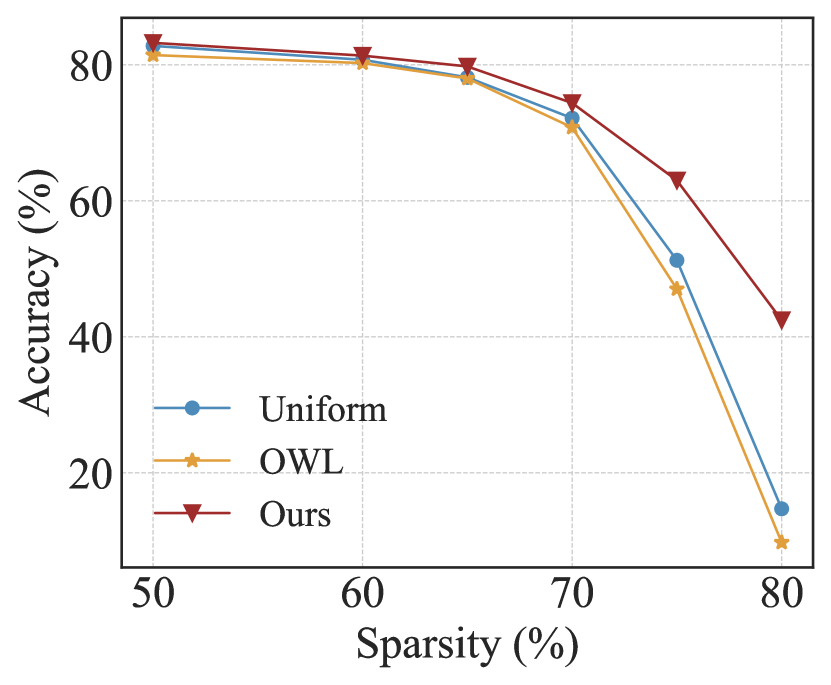
Figure 4: ImageNet-1K accuracy ($\uparrow$) of the sparse ConvNext model pruned to various sparsity levels by AlphaPruning and other baseline methods, without fine-tuning.

More LLM architectures.

To demonstrate that the effectiveness of AlphaPruning is robust across various more advanced LLMs, we also apply AlphaPruning to LLaMA-3-7B, Vicuna-7B Zheng et al. (2024), and Mistral-7B Jiang et al. (2023). The results in Table 5.3 show that, as a general method, AlphaPruning can consistently achieve performance improvement across different architectures. Results for OPT families can be found in Appendix H.5.

Integration with other compression techniques.

To demonstrate the generalizability of our non-uniform layerwise sparsity, we integrated AlphaPruning with three prominent LLM compression methods: N:M sparsity, structured pruning, and quantization. In Appendix H.6, we examine a mixed N:8 sparsity setup using DominoSearch Sun et al. (2021) as well as combine AlphaPruning with structured pruning methods LLM-Pruner Ma et al. (2023) and OSSCAR Meng et al. (2024). In Appendix H.7, we merge our method with mixed-precision quantization as  Tang et al. (2022). Across these configurations, AlphaPruning consistently enhances the performance of baseline methods.

Vision models.

To illustrate AlphaPruning in a broader context, we study how it performs against other methods for determining layerwise sparsity on CV tasks, where non-uniform layerwise sparsity has been widely used. We consider two modern CV architectures: ViT Dosovitskiy et al. (2020) and ConvNext Liu et al. (2022b). We adopt Wanda as the pruning approach and compare AlphaPruning with uniform layerwise sparsity and OWL. We present the results on ConvNext in Figure 4 and provide more results on DeiT and ViT models in Appendix H.9. These results affirm that AlphaPruning effectively allocates layerwise sparsities in CV tasks as well, where OWL significantly underperforms AlphaPruning due to the lack of outlier features. This indicates HT metrics are more general than outlier metrics.

5.4 Analyzing LLM pruning via HT-SR perspective

First, we investigate the distribution of layerwise sparsities allocated by the heavy-tailed metric PL_Alpha_Hill. Then, we study how the PL_Alpha_Hill metric as a measure of model quality (based on HT-SR theory) changes before and after pruning. In particular, we show that the proposed method, AlphaPruning, effectively controls the damage of pruning to model quality, resulting in a more favorable distribution (lower mean) of PL_Alpha_Hill among the model layers compared to the baseline pruning method. Our primary focus is on LLaMA, with additional analyses on other LLMs provided in Appendix D.1.

Analyzing the layerwise sparsity distribution.

We elaborate on the layerwise sparsities assigned by AlphaPruning and heavy-tailed metric PL_Alpha_Hill. The metric and sparsities results of LLaMA-7B are presented in Figure 5. We can observe that, the blue bar histograms demonstrate that different layers of one model show diverse PL_Alpha_Hill values, this indicates that these layers are not equally well-trained. This conclusion is based on prior research on heavy-tails in weight matrices Martin et al. (2021); Martin and Mahoney (2019), this metric measures the heavy-tailed structure within the correlation matrix. This measurement indicates the amount of correlation among the weight matrix elements, with strong correlations leading to a more heavy-tailed empirical spectral density. Such a structure is often seen as a result Wang et al. (2024) of extracting various useful correlations (or features) from data during optimization.

Consequently, smaller PL_Alpha_Hill layers (more heavy-tailed) contain a greater number of learned correlations. The larger PL_Alpha_Hill layers (less heavy-tailed) tend to retain fewer learned correlations, remaining closer to the random initialization state. Figure 5 shows that AlphaPruning suggests that large PL_Alpha_Hill layers with fewer learned correlations should be allocated with larger sparsity, or being pruned more, while those small PL_Alpha_Hill layers should be allocated with lower sparsity.

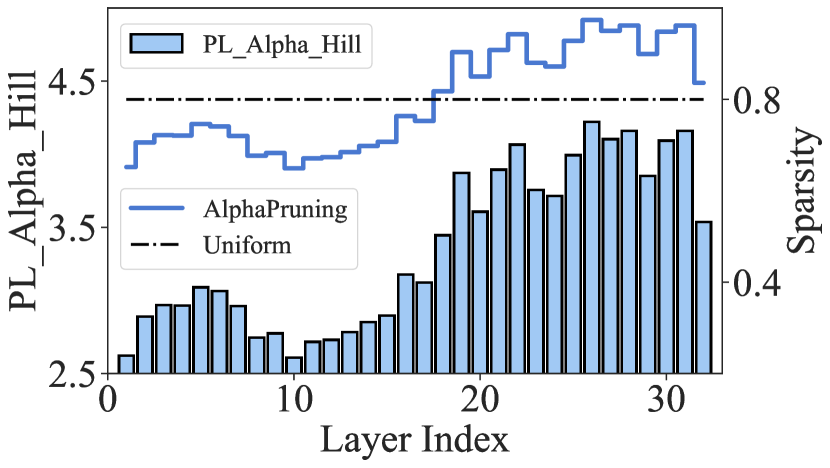
Figure 5: Comparing layerwise sparsities of AlphaPruning and uniform sparsities, at 80% global sparsity on LLaMA-7B. The curves represent the layerwise sparsities, which are determined by PL_Alpha_Hill values shown by the histograms.

Analyzing PL_Alpha_Hill affected by pruning.

We investigate how PL_Alpha_Hill values change before and after pruning. According to HT-SR Theory Yang et al. (2023); Martin et al. (2021), models or layers of higher quality typically exhibit lower PL_Alpha_Hill values. As observed in Figure 6(a), dense LLaMA models (depicted in gray) consistently show a lower mean PL_Alpha_Hill, with larger models demonstrating an even lower mean. Furthermore, we can see both pruning methods lead to increments of the metric value, as pruning is often seen as damaging the quality of the model, the changes are well correlated with the perplexity. More interestingly, AlphaPruning not only outperforms the Uniform pruning in perplexity, but it also leads to a smaller mean of PL_Alpha_Hill. Figure 6(b) delves deeper into this phenomenon by visualizing the metric value in a layer-wise manner. It is noticeable that AlphaPruning leads to lower PL_Alpha_Hill than the uniform pruning among the first several blocks. This is due to the mechanism (Figure 5) by which our method prunes the model based on the layer-wise PL_Alpha_Hill, and prunes less on these more heavy-tailed layers.

Based on these results, we can conclude that: (1) pruning a model to a larger sparsity generally hurts the model’s task performance (e.g., perplexity), and this coincides with decreased model quality, as measured by PL_Alpha_Hill; and (2) a better pruning method such as AlphaPruning can obtain a sparse model with a smaller mean of layer-wise PL_Alpha_Hill, and this is achieved by pruning less aggressively in the dense layers with lower PL_Alpha_Hill layers.

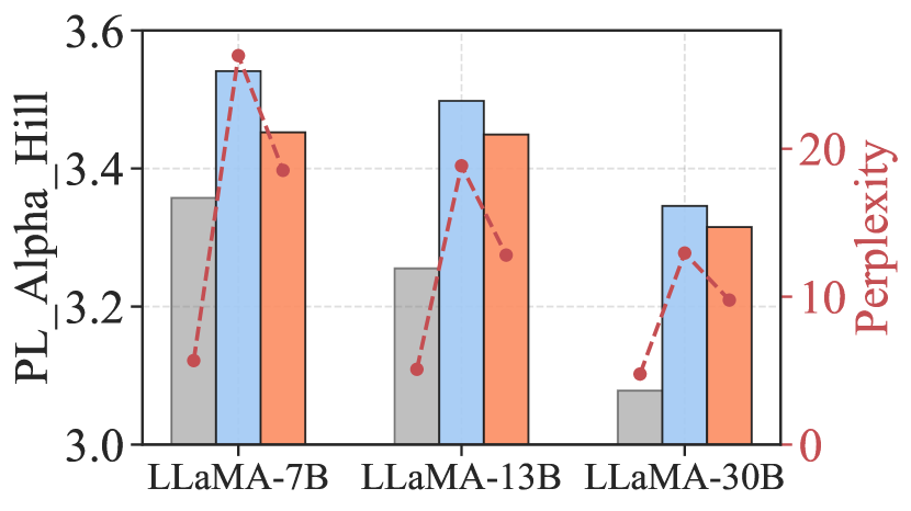
(a) Model-wise heavy-tail analysis

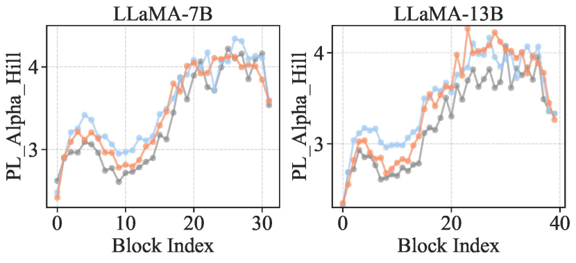
(b) Layer-wise heavy-tail analysis

Figure 6: Analyzing the heavy-tail metric PL_Alpha_Hill (lower the better by HT-SR theory) and performance metric WikiText validation perplexity (lower the better) before and after pruning by baseline uniform pruning and AlphaPruning. (a) The metric value is reported by averaging over all layers within each model. The dashed lines represent the perplexity and the histograms represent the PL_Alpha_Hill value. (b) The metric is reported by averaging all the matrices within each LLM layer.

Connections with Low-rank Approximation.

A commonly used compression technique that also involves analyzing the eigenspectrum of the weights is Low-Rank Approximation (LRA) Zhang et al. (2015); Wen et al. (2017); Xu et al. (2019); Barsbey et al. (2021). We examine the apparent connection between our method, AlphaPruning, and LRA from two perspectives. First, we study the relationship between the ESD used in our method and the low-rank properties often used in LRA, where we use PL_Alpha_Hill to measure HT and Stable_Rank to measure low-rank properties. Second, we study the differing layer-wise assignment strategies adopted by the two methods. Finally, we discuss how our findings relate to those of Barsbey et al. (2021), a paper closely related to ours, showing that the results from both studies complement each other, offering different yet compatible insights.

For the first point, we find a strong positive correlation between the HTed properties and the low-rank properties used in LRA: as the ESD becomes more HTed, it also becomes more low-ranked. To demonstrate this, we sampled eigenvalues from an IID Pareto distribution with varying tail indices to form ESDs and then measured Stable_Rank on these ESDs. A lower PL_Alpha_Hill indicates a more HTed distribution, while a lower Stable_Rank indicates a more low-ranked structure. Figure 7(a) shows that Stable_Rank and PL_Alpha_Hill are positively correlated across different matrix sizes, suggesting a relationship between HTed and low-ranked properties. In Figure 7(b), we further verify this by measuring PL_Alpha_Hill and Stable_Rank across different layers of the pre-trained LLaMA-7B model. The results reveal that both metrics follow a similar trend: shallow layers show lower values, while deeper layers exhibit higher values, indicating consistent behavior across layers. Therefore, we can see that the key metrics used in AlphaPruning and LRA are highly correlated.

For the second point, we clarify that the strategies for assigning higher or lower compression to HTed or low-ranked layers differ between AlphaPruning and LRA. AlphaPruning assigns lower compression ratios (less sparsity) to HTed layers. In contrast, LRA assigns higher compression to low-ranked layers Zhang et al. (2015); Wen et al. (2017); Xu et al. (2019), which, as established earlier, tend to be HTed. Therefore, the two methods seemingly use different procedures in assigning layerwise compression ratios. In Figure 7(c), we empirically verify that, for LRA, assigning higher compression to HTed layers is indeed more beneficial than its opposite for LLMs, as shown by the results of applying both to LLaMA-7B models. This finding is opposite to the assignment method used in AlphaPruning. We hypothesize that these differences arise from the distinct mechanisms and principles of each method. In more detail, AlphaPruning, which is pruning-based, removes elements from the weight matrices, affecting the entire eigenspectrum. LRA, however, removes only the smallest eigenvalues, leaving the larger eigenvalues intact. The guiding principle of AlphaPruning is also different from LRA. It aims to make the model more deterministic and less random by preserving weights corresponding to well-trained layers. It does this by preserving HTed layers that contain more signals and removing light-tailed layers that, according to HT-SR theory, resemble randomly initialized weight matrices. In some sense, it is similar to how decision trees choose branches to reduce entropy. LRA, on the other hand, focuses on applying more compression on low-rank matrices where the largest eigenvalues dominate. This allows for minimal impact on reconstruction loss when removing small eigenvalues.

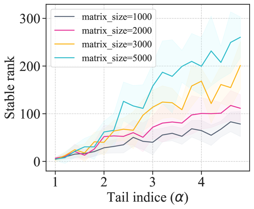
(a) Stable_Rank of ESD sampled from Pareto distribution

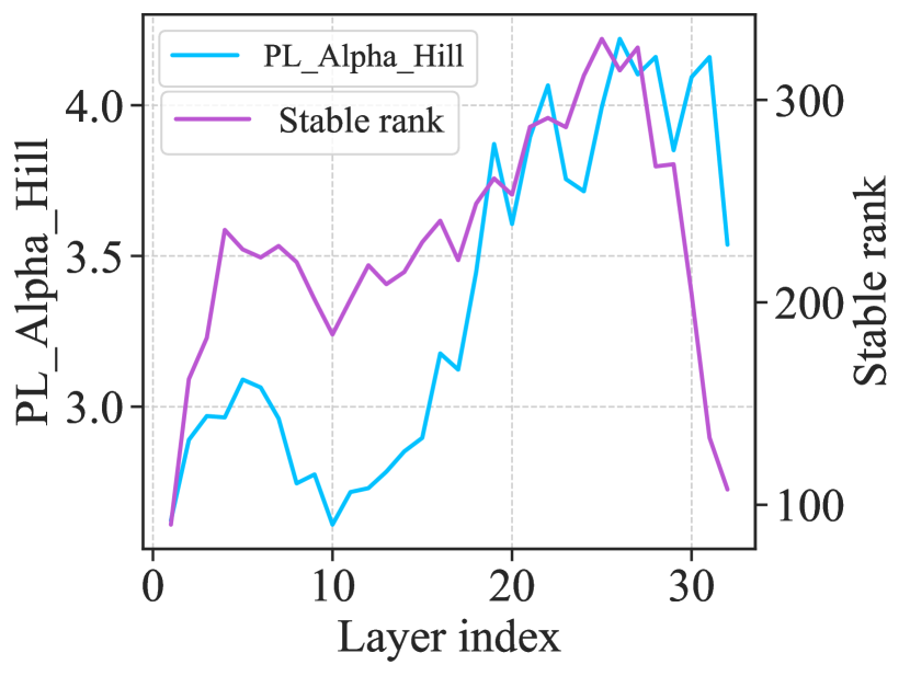
(b) Layerwise metric values of LLaMA-7B

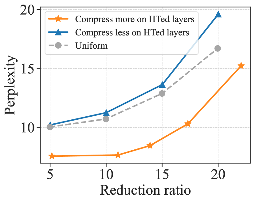
(c) Comparing layer-wise assignment strategies for LRA

Figure 7: Analyzing ESD properties and assignment strategies for LRA. (a) Stable_Rank and PL_Alpha_Hill show a similar pattern (the more heavy-tailed, the more low-ranked) across different ESDs sampled from Pareto distribution. (b) The layer-wise PL_Alpha_Hill and Stable_Rank of the LLaMA-7B model exhibit a similar trend. (c) Comparing two assignment strategies for LRA, and “Compress more on HTed layers” is better. This finding is opposite to pruning-based methods, which find that “Compress less on HTed layers” is better.

Lastly, Barsbey et al. (2021) concluded that models with lower HT measures are generally more compressible than other models, focusing on cross-model comparisons. In contrast, our work examines compressibility within a single model and suggests that, within a model, layers with lower HT values are less compressible than other layers. Our insight supports layer-wise pruning strategies, such as AlphaPruning, which applies less compression to more HTed layers. We empirically confirm that both conclusions are complementary. Following the setup of Barsbey et al. (2021), detailed in Appendix D.3, we reproduced their findings in Figure 10 and demonstrated compatibility with AlphaPruning’s assignment strategies. We generated four trained models with varying model-wise HT measures and pruned them using different layer-wise strategies. The results verified that models with lower HT metrics are more compressible. In Figure 11, we further validated our findings using the same models. Among four models with varying model-wise HT values, we confirmed that HTed layers are less compressible and that pruning HTed layers less (which AlphaPruning does) is more effective.

6 Conclusion

We have used methods from HT-SR Theory to develop improved methods for pruning LLMs. The basic idea is to analyze the ESDs of trained weight matrices and to use shape metrics from these ESDs to measure how much to prune a given layer, with less well-trained layers, as measured by these shape metrics from HT-SR Theory, being pruned more aggressively. Our extensive empirical evaluation demonstrates that AlphaPruning offers a straightforward yet effective way of determining the layer-wise sparsity ratios. Our analysis reveals that different layers of an LLM are not equally trained (typically, the ESDs of early layers are more HT and thus are more well-trained, compared to later layers), and that shape-based ESD metrics work better for layer quality prediction in pruning pipelines than scale-based ESD metrics. AlphaPruning achieves higher sparsity, without severely hurting performance, and also smaller values of PL_Alpha_Hill after pruning. AlphaPruning is also compatible with multiple existing LLM pruning methods and is expected to be integrated with future ones, as long as the methods allow specifying layerwise ratios.

Appendix

Appendix A Impact Statements

This paper leverages HT-SR Theory to design improved layerwise pruning ratios for LLMs. Although the proposed method could be applied to compress models with adverse applications, we do not see any immediate negative societal impacts stemming from the algorithm itself. Indeed, we see a lot of societal value in proposing our method to the community. Through the implementation of effective layerwise sparsity, we can achieve substantial reductions in the parameters of LLMs while retaining their functionality. Consequently, this advancement facilitates the deployment of LLMs in resource-constrained devices, accelerates the predictions for resource-limited LLM services, and contributes to the sustainability of LLM technologies.

Appendix B Limitation

This paper’s empirical evaluation focuses on post-training pruning methods without fine-tuning, in alignment with recent research in LLM pruning, such as OWL, Wanda, and SparseGPT. This is due to the substantial computational resources required to restore heavily pruned LLMs to their original performance. Nonetheless, our experiments with limited fine-tuning have demonstrated that the proposed pruning method can achieve only a mild performance drop while yielding significant efficiency improvements.

Appendix C Definitions of HT-SR metrics

Here, we define the shape metrics, beyond PL_Alpha_Hill, that we use in our analysis.

• (Alpha_Hat) The Alpha_Hat metric Martin et al. (2021) has been shown to be effective at predicting generalization. It is the variant of PL exponent $\alpha$ (PL_Alpha) weighted by the log maximum eigenvalue $\log\lambda^{\text{max}}$(log_spectral_norm):

  $$\texttt{Alpha\_Hat}=\alpha\log\lambda^{\text{max}}.$$ (5)

• (Stable_Rank) The Stable_Rank metric is a norm-adjusted measure of the scale of the ESD, and previous work Yang et al. (2023) has shown its strong correlation with PL_Alpha. For a weight matrix $\mathbf{W}$, it can be calculated as:

  $$\texttt{Stable\_Rank}=\left\|\mathbf{W}\right\|^{2}_{F}/\left\|\mathbf{W}\right\|_{2}^{2}.$$ (6)

• (Entropy) For a weight matrix $\mathbf{W}$, the Entropy metric is defined as

  $$\texttt{Entropy}=\frac{-1}{\log{R(\mathbf{W})}}\sum_{i}p_{i}\log{p_{i}}.$$ (7)

  where $p_{i}=v_{i}^{2}/\sum_{i}v_{i}^{2}$, $v_{i}$ is the $i$-th singular value of $\mathbf{W}$, and $R(\mathbf{W})$ refers to the rank of $\mathbf{W}$.

Appendix D Further analysis of results

D.1 Post-pruning layer-wise heavy-tail analysis

We investigate layer-wise PL_Alpha_Hill values after pruning by Uniform pruning and AlphaPruning on more advanced LLMs (LLaMA-V3-8B, Vicuna-7B, Mistral-7B). According to HT-SR Theory, models or layers of higher quality typically exhibit lower PL_Alpha_Hill values. As observed in Figure 8, AlphaPruning leads to a smaller layer-wise PL_Alpha_Hill. This is due to the mechanism (1) by which our method prunes the model based on the layer-wise PL_Alpha_Hill, and prunes less on these more heavy-tailed layers.

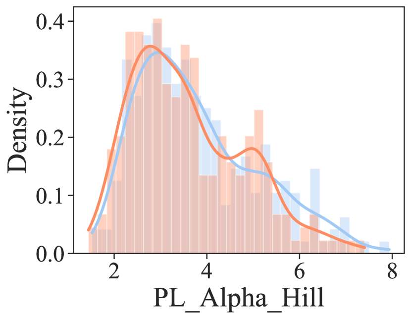
(a) LLaMA-V3-8B

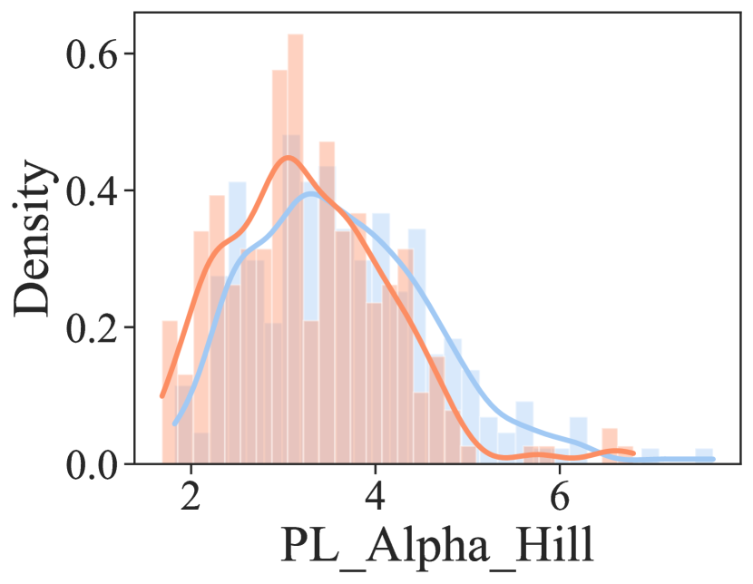
(b) Vicuna-7B

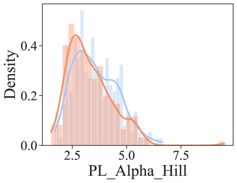
(c) Mistral-7B

Figure 8: Analyzing the layer-wise heavy-tail metric PL_Alpha_Hill (lower the better by HT-SR theory) after pruning by baseline uniform pruning and AlphaPruning.

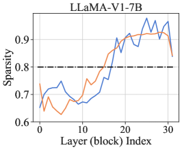
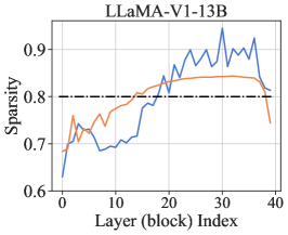
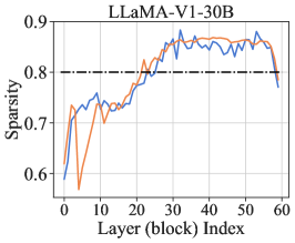
Figure 9: Comparing layer-wise sparsity distributions allocated by AlphaPruning (blue, ours) and OWL (orange). While both methods show similar overall trends, AlphaPruning generates a more granular distribution with distinct differences between consecutive layers.

D.2 Comparison with other LLM layer quality metrics

In addition to AlphaPruning proposed in our work, Gromov et al. (2024); Men et al. (2024) are other studies that investigated methods that measure whether a layer is well-trained or not, demonstrating LLMs layers are not equally well-trained. Gromov et al. (2024) developed a method that assesses the similarity between the representations at different layers, defined as the angular distance between feature vectors. They found that deeper layers are more similar to their neighboring layers than shallow layers, suggesting that LLMs may not fully use the parameters in these deeper layers, indicating these layers are not well-trained. Similarly, Men et al. (2024) introduced a metric called Block Influence, which measures the impact of each transformer block on hidden states to gauge layer significance. Their findings showed varying degrees of ineffectiveness/redundancy across layers, suggesting that these layers are not well-trained.

Besides, in Figure 9, we compare the sparsity allocation of AlphaPruning with OWL. We show that the general trends of sparsity distribution generated by the two methods are similar, with lower sparsities allocated to earlier layers and higher sparsities allocated to deeper layers. However, our method produces a more granular distribution with clearer distinctions between consecutive deep layers, resulting in improved pruning performance.

D.3 Comparison with conclusions of Barsbey et al. (2021)

Barsbey et al. (2021) studied a problem related to ours, and they showed that models with more HTed weights had improved compressibility. We adopt the experimental setup of Barsbey et al. (2021), training fully connected networks (FCNs) with six hidden layers on the CIFAR-10 dataset. The HT measure used in their study referred to as Alpha, quantifies the HTed structure of the weight parameters. The model-wise HT measure is influenced by the “temperature”, defined as the ratio of learning rate to batch size. Higher temperatures yield models with lower HT measures. Our first experiment reproduces the finding of Barsbey et al. (2021), comparing the compressibility of models with varying model-wise HT measures. It also tries to verify if the conclusions hold when using our proposed layer-wise strategies. The results shown in Figure 10 support our hypotheses. The second experiment compares the effectiveness of these layer-wise strategies and also checks if the findings are consistent across models with different model-wise HT measures. The results shown in Figure 11 again confirm the hypothesis.

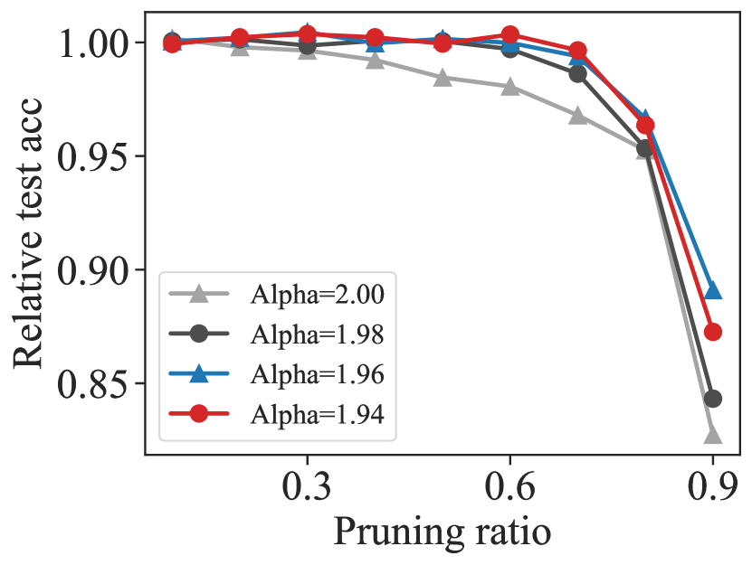
(a) Uniform Pruning

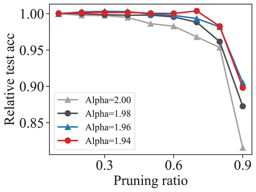
(b) AlphaPruning

Figure 10: Comparison of pruning models with varying model-wise HT measures (Alpha). Models with higher HT measures are more prunable using both Uniform pruning and AlphaPruning. Relative accuracy is calculated as the post-pruning accuracy divided by the pre-pruning accuracy. The experiments used FCNs trained on CIFAR-10.

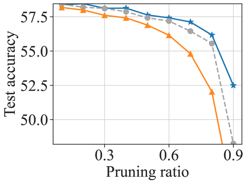
(a) Alpha=2.00

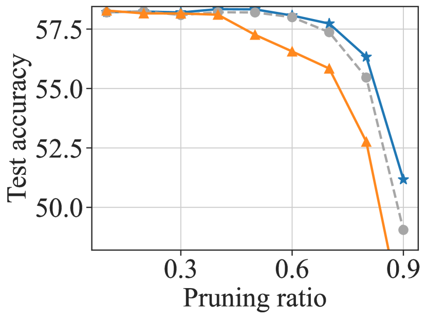
(b) Alpha=1.98

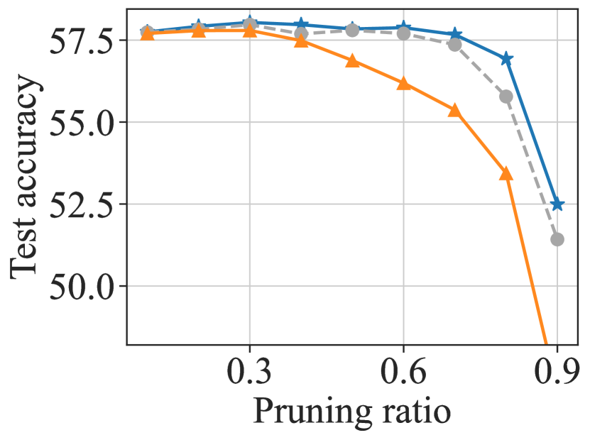
(c) Alpha=1.96

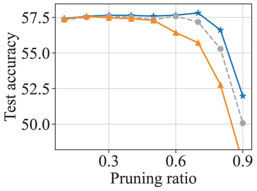
(d) Alpha=1.94

Figure 11: Comparison of our proposed layer-wise assignment strategy with other strategies on models with varying model-wise HT measures. “Compress less on HTed layer” (AlphaPruning) consistently outperforms Uniform pruning across different models, while “Compress more on HTed layer” leads to worse performance compared to Uniform pruning. The experiments used FCNs trained on CIFAR-10.

Appendix E Ablation study of sparsity allocation

In Section 4.3, we introduced the range hyperparameters $s_{1}$ and $s_{2}$ to control the non-uniformity of layer-wise sparsities. To simplify, we define $\tau$ such that $s_{1}=1-\tau,s_{2}=1+\tau$. AlphaPruning allocates sparsity on a “per-block” basis, where all matrices within a block receive the same sparsity, determined by averaging the PL_Alpha_Hill values across matrices within that block. Alternatively, sparsity can be allocated on a “per-matrix” basis, allowing different sparsities for individual matrices based on their PL_Alpha_Hill values. The ablation study on comparing per-matrix and per-block choices is presented in E.1. The ablation study on comparing different mapping functions is shown in E.2.

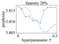
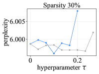
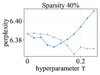
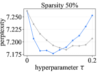
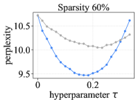
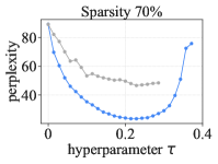
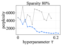
Figure 12: Ablation study on sparsity allocation function hyperparameter $\tau$. We use Wanda to prune LLaMA model using AlphaPruning with both per-matrix and per-block allocation methods.

E.1 Per-matrix vs. per-block

In Figure 12, we compared per-matrix and per-block sparsity allocation across different values of the hyperparameter $\tau$, using Wanda. The results show a regime transition in pruning effectiveness between the two methods. For sparsity levels below 50%, the per-matrix approach (gray lines) achieves lower perplexity, indicating better performance. However, for sparsity values of 50% and above, the per-block method (blue line) performs better. We further focused on high sparsity 70%, as higher sparsity is more important to provide efficiency improvements. Specifically, we evaluated both per-matrix and per-block methods in combination with various intra-layer pruning techniques. Table E.1 shows that the per-block method consistently outperforms the per-matrix method when used in conjunction with three intra-layer pruning techniques.

Additionally, we analyzed the differences between MLP and Attention matrices by visualizing average PL_Alpha_Hill values for seven types of weight matrices in LLaMA-7B, as shown in Figure E.1. The results indicate that query and key matrices have lower PL_Alpha_Hill values, suggesting they are less prunable. Based on this insight, we developed a new allocation strategy called “Mixed”, which combines per-block and per-matrix approaches. As defined, Mixed first assigns a block-wise pruning ratio using the per-block method, then refines it within each block using per-matrix allocation. Table E.1 demonstrates that this Mixed approach provides further marginal improvements over both per-matrix and per-block methods.

Method	Uniform	Per-matrix	Per-block	Mixed
Magnitude	48419.13	7384.13	231.01	177.86
Wanda	85.77	58.71	23.86	22.46
SparseGPT	26.30	25.10	18.54	18.32

Table 7: Comparing perplexity of sparse LLaMA-7B (sparsity=70%) pruned by four types of sparsity allocation method.

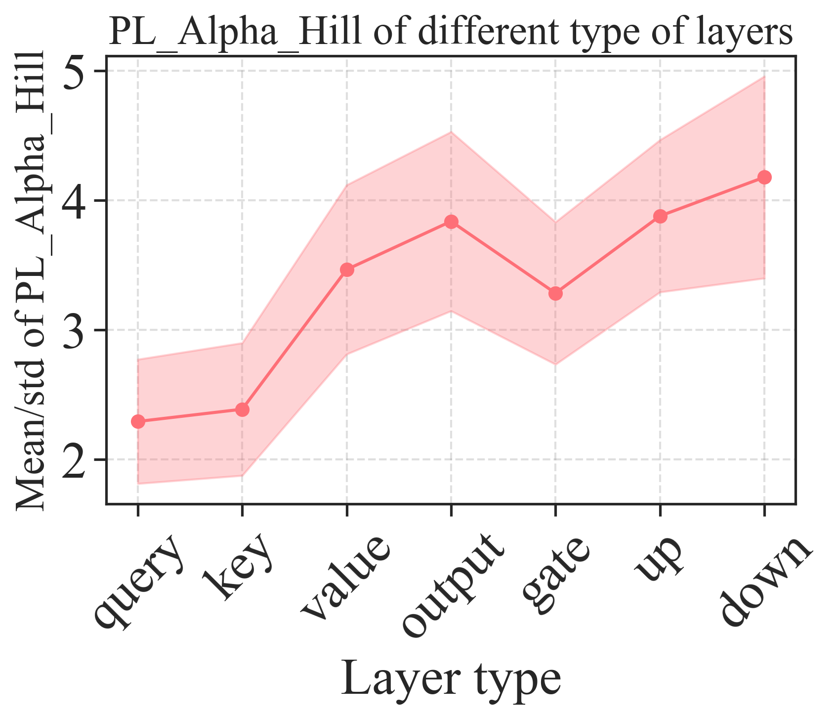
Figure 13: Averaged PL_Alpha_Hill metric values for seven types of weight matrices in LLaMA-7B.

E.2 Different mapping functions

We provide ablation studies on the choices of sparsity assignment function. We implemented the logarithmic method and compared it with the linear mapping function used in our current approach, as shown in Figure 14. The results show that both methods perform similarly when combined with Wanda, but linear mapping slightly outperforms the proposed logarithmic method when combined with SparseGPT.

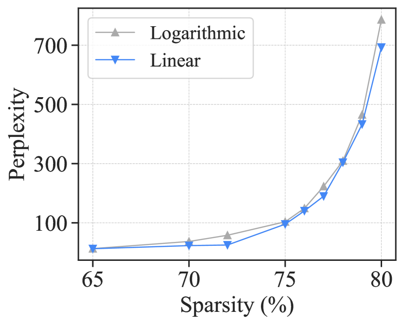
(a) Wanda

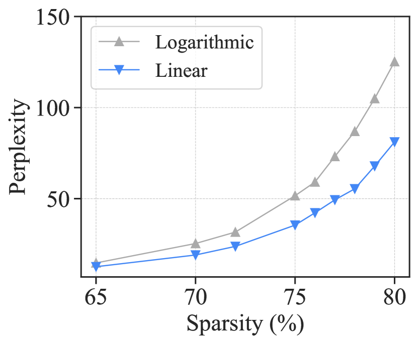
(b) SparseGPT

Figure 14: Comparing different mapping functions. Linear (ours) refers to the linear mapping function that is used in our current method. Logarithmic refers to computing the logarithmic of metrics before linear mapping. The model is LLaMA-V1-7B. (a-b) refers to combining different intra-layer pruning methods.

Appendix F Hypterparamter setting

Here, we provide the values of $\tau$ used in the experiments, as shown in Table 8.

	Method
Model	Magnitude	Wanda	SparseGPT
LLaMA-7B	0.3	0.2	0.2
LLaMA-13B	0.5	0.3	0.3
LLaMA-30B	0.4	0.3	0.3
LLaMA-65B	0.4	0.3	0.3
LLaMA2-7B	0.5	0.3	0.2
LLaMA2-13B	0.4	0.3	0.3
LLaMA2-70B	0.4	0.3	0.3

	Sparsity
Model	40%	50%	60%	70%	80%
ViT-B	0.3	0.3	0.3	–	–
ViT-L	0.3	0.3	0.3	–	–
DeiT-S	0.4	0.4	0.4	–	–
DeiT-L	0.3	0.3	0.3	–	–
ConvNext	0.1	0.1	0.2	0.2	0.2

Table 8: Left: Hyperparameters setting for results in Section 5.2. We report the optimal $\lambda$ after a small hyperparameter sweep within the range of $\tau\in$ [0.2, 0.3, 0.4, 0.5]. Right: Hyperparameters setting for results in Section 5.3 for Vision Transformers at 40%, 50%, 60% sparsity. We report the optimal $\lambda$ after a small hyperparameter sweep within the range of $\tau\in$ [0.1, 0.2, 0.3, 0.4, 0.5].

Appendix G More baseline comparison

For assigning layerwise sparsity ratios, we compare AlphaPruning with other methods. In this section, we provide definitions and details of these methods:

• Uniform. Zhu and Gupta (2017) Every layer pruned with the same target sparsity.

• Global Frankle and Carbin (2018). A global threshold uniformly applied to all layers to satisfy the overall sparsity requirement. The specific layerwise sparsity is automatically adjusted based on this threshold.

• ER Mocanu et al. (2018). The sparsity of the convolutional layer is scaled proportionally to $1-\frac{h^{l-1}+h^{l}}{h^{l-1}\times h^{l}}$ where $h^{l}$ refers to the number of neurons/channels in layer $l$.

• ER-Plus Liu et al. (2022a). ER-Plus modifies ER by forcing the last layer as dense if it is not, while keeping the overall parameter count the same.

• LAMP Lee et al. (2020). This method modifies Magnitude-based pruning by rescaling the importance scores in a layer by a factor dependent on the magnitude of surviving connections in that layer.

• OWL Yin et al. (2023). A non-uniform layerwise sparsity based on the distribution of outlier activations in LLMs, probing the possibility of pruning LLMs to high sparsity levels.

We adopt Wanda and SparseGPT as the pruning approach. The results are presented in Table 9 and Table 10, which indicate that AlphaPruning significantly outperforms all baseline methods in relatively high-sparsity regimes. Besides, we have conducted additional experiments using the “layerwise error thresholding” method, where each layer is pruned sequentially as specified in  Zhuang et al. (2018); Ye et al. (2020). We have also implemented the rank selection method as specified in Section 5.2 of  El Halabi et al. (2022). We present the updated experimental results in Table 11. We observe that our method outperforms all the other baselines.

Method/Perplexity ($\downarrow$)	10%	20%	30%	40%	50%	60%	70%	80%
Global	14.11	3134	10293	10762	14848	17765	5147	39918.56
LAMP	5.69	5.78	5.98	6.3912	7.57	12.86	185.52	15647.87
LAMP (per-block)	5.70	5.82	6.00	6.40	7.25	10.95	98.77	7318.08
ER	5.70	5.81	6.03	6.57	7.80	12.41	119.66	6263.79
ER-Plus	5.70	5.82	6.05	6.62	8.00	14.04	229.17	6013.91
Uniform	5.70	5.82	6.00	6.39	7.26	10.63	84.52	5889.13
OWL	5.70	5.80	6.01	6.39	7.22	9.35	24.56	1002.87
Ours	5.69	5.81	6.00	6.37	7.18	9.47	23.86	698.56

Table 9: WikiText validation perplexity ($\downarrow$) of LLaMA-7B pruned by different allocation methods at various global sparsities using Wanda. AlphaPruning outperforms other layerwise sparsity at high sparsity range.

Method/Perplexity ($\downarrow$)	10%	20%	30%	40%	50%	60%	70%	80%
LAMP	5.69	5.78	5.96	6.34	7.37	11.27	31.96	274.73
LAMP (per-block)	5.70	5.80	5.96	6.33	7.22	10.45	27.05	224.32
ER	5.70	5.81	6.02	6.49	7.54	11.29	30.20	258.63
Uniform	5.69	5.89	5.96	6.32	7.22	10.56	26.30	188.11
OWL	5.71	5.81	5.97	6.35	7.22	9.51	19.49	84.94
Ours	5.69	5.81	5.99	6.36	7.30	9.73	18.44	81.98

Table 10: Perplexity ($\downarrow$) of pruning LLaMA-7B into various global sparsities using SparseGPT. We compare our method with three other baseline sparsity allocation methods.

Method	Global sparsity	Perplexity ($\downarrow$)	Zero-shot Accuracy ($\uparrow$)
Uniform	70%	26.30	41.52
Layerwise error thresholding	70%	32.54	41.24
Rank selection	70%	21.34	42.90
Ours	70%	18.54	45.48

Table 11: Comparing our method to other layerwise sparsity baseline methods in pruning LLaMA-7B into 70% sparsity. The perplexity is evaluated on the WikiText validation set. The zero-shot accuracy is averaged over 7 downstream tasks. Each method is combined with SparseGPT.

Appendix H Complementary Experimental Results

H.1 Shape metrics versus scale metrics on Vision Transformers

We further evaluate different metrics for computing layerwise sparsity on Vision Transformers. Shape metrics, including Alpha_Hat, Entropy, PL_Alpha_Hill, and Stable_Rank, are obtained from the shapes of the ESDs. Scale metrics, including Frobenius_Norm and Spectral_Norm, are norm-based metrics measuring the scale of weights matrices (which can also be obtained from the ESD). The results shown in Table 12 align with the results in LLMs that shape metrics outperform scale metrics on allocating layerwise sparsity and PL_Alpha_Hill performs the best.

Metric used for	ViT-L 16/224 accuracy ($\uparrow$)			DeiT-S 16/224 accuracy ($\uparrow$)
layerwise pruning ratios	40%	50%	60%	40%	50%	60%
Uniform	76.05	68.73	39.45	75.62	68.98	50.49
Frobenius_Norm	76.15	68.93	37.46	76.62	72.21	58.93
Spectral_Norm	75.99	67.72	32.98	75.97	70.13	53.76
Entropy	76.37	71.17	49.09	76.77	71.63	58.23
Stable_Rank	75.91	68.93	41.26	75.63	68.64	46.86
Alpha_Hat	77.11	72.01	52.56	76.94	72.10	59.78
PL_Alpha_Hill	76.86	72.12	55.62	77.07	72.38	60.92

Table 12: Evaluating shape metrics versus scale metrics on allocating layerwise sparsities on Vision Transformers. Shape metrics are obtained from the shapes of the ESDs. Scale metrics are norm-based metrics measuring the scale of weights matrices (which can also be obtained from the ESD). We choose two models, ViT-L and DeiT-S, and the results are shown on ImageNet-1K accuracy without fine-tuning. We observe that shape metrics outperform scale metrics and PL_Alpha_Hill performs the best.

H.2 More results on other efficiency metrics

To further demonstrate the benefits of our approach, we provide results in other practical efficiency metrics such as FLOPs. Compared with uniform sparsity ratios, our approach is able to achieve a better performance-FLOPs trade-off. We have provided new results of FLOPs in Figure 15.

Table 13 summarizes the results from Figure 15. We show that, compared to uniform pruning, our method can achieve significant FLOPs reduction when pruned LLMs are compared at similar perplexity.

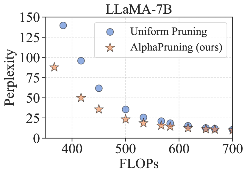
(a) Broader perplexity range

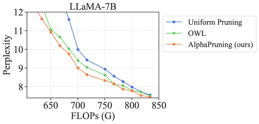
(b) Lower perplexity range

Figure 15: Additional results of FLOPs measurement on the LLaMA-7B pruned by Uniform and our method with SparseGPT.

Uniform	Perplexity ($\downarrow$)	9.80	18.58	21.06	25.70	35.57	61.76	95.82
	FLOPs ($\downarrow$)	716.80	583.49	566.82	533.49	500.16	450.17	416.84
Ours	Perplexity ($\downarrow$)	9.78	15.67	18.63	23.39	35.74	49.94	87.81
	FLOPs ($\downarrow$)	700.14	566.82	533.49	500.16	450.17	416.84	366.85

Table 13: Additional results of FLOPs measurement on the LLaMA-7B pruned by Uniform and our method with SparseGPT.

H.3 Controlling the minimum layer sparsity for memory-limited hardware

To enhance the adaptability of our method to hardware, we demonstrate that our method allows for controlling the minimum sparsity, by adjusting the values of $s_{1}$ and $s_{2}$. Additionally, Table 14 demonstrates that increasing the minimum sparsity by changing $s_{1}$ and $s_{2}$ doesn’t diminish the advantages of our method, compared to the uniform pruning baseline.

Recall that the sparsity of the layer of the model can be determined by Eqn. 4. Increasing $s_{1}$ leads to a higher minimum sparsity $\eta s_{1}$, while maintaining the same global sparsity $S$. Table 14 displays the results of adjusting $s_{1}$ and $s_{2}$ to increase the minimum sparsity while maintaining the global sparsity at 70%. At a minimum sparsity of 57%, our method achieves the lowest perplexity. Even when the minimum sparsity is raised to 67%, nearing the uniform pruning baseline, our method still attains a perplexity of 49.6, which is 36.17 points lower than that of uniform pruning (85.77).

Method	Global sparsity $S$	Minimum sparsity $\eta s_{1}$	Perplexity
Uniform	70%	70%	85.77
Ours	70%	50%	33.46
Ours	70%	55%	26.19
Ours	70%	57%	23.79
Ours	70%	60%	27.18
Ours	70%	65%	40.22
Ours	70%	67%	49.60

Table 14: Increasing the minimum sparsity of our method, while maintaining a global sparsity of 70%, still yields performance improvements compared to a uniform sparsity ratio. We present the WikiText validation perplexity for LLaMA-7B pruned by both the Uniform method and our method, in conjunction with Wanda.

H.4 Computational complexity of AlphaPruning

The computational complexity of AlphaPruning is not large because the most computation-intensive aspect of our method involves performing SVD decomposition on weight matrices, which can be further optimized through parallel processing. Table 15 presents the runtime of our AlphaPruning and an optimized version that uses parallel processing. The increase in runtime is reasonable, at 32.44% with Wanda and 8.2% with SparseGPT. These experiments were conducted on pruning LLaMA-7B to 70% sparsity. The testing platform used A40 GPUs and an AMD EPYC 7713 64-Core CPU.

Method	Ours	Original method (second)	Percentage of runtime increase (%)
Wanda	–	176	0%
Wanda $w.$ Ours (1 GPU)	462	178	259.55%
Wanda $w.$ Ours (8 GPUs)	57	178	32.44%
SparseGPT	–	699	0%
SparseGPT $w.$ Ours (1 GPU)	462	695	66.47%
SparseGPT $w.$ Ours (8 GPUs)	57	695	8.2%

Table 15: Runtimes of our method combined with Wanda and SparseGPT on LLaMA-7B.

H.5 OPT family

In addition to LLaMA and LLaMA-2, we conduct experiments with OPT Zhang et al. (2023). Table 16 shows the results of comparing our method to uniform sparsity when both are combined with magnitude pruning. Table 17 shows the same comparison when both combined with Wanda Sun et al. (2023) /SparseGPT Frantar and Alistarh (2023b). In most of the cases, our method outperforms the baseline method and achieves lower perplexity.

Method	Sparsity	OPT-125M	OPT-350M	OPT-2.7B	OPT-6.7B
magnitude	40%	54.60	40.19	30.31	31.89
magnitude $w.$ Ours	40%	52.29	38.20	22.31	19.53
magnitude	50%	193.35	97.79	265.20	968.72
magnitude $w.$ Ours	50%	173.01	95.61	159.44	224.91

Table 16: The perplexity of OPT models pruned by uniform sparsity and our method combined with magnitude pruning. The perplexity is evaluated on WikiText validation set.

Method	Sparsity	OPT-125M	OPT-350M	OPT-2.7B	OPT-6.7B
Wanda	70%	334.58	758.81	265.20	158.38
Wanda $w.$ Ours	70%	269.80	654.17	159.44	40.81
SparseGPT	70%	226.30	146.45	26.95	20.38
SparseGPT $w.$ Ours	70%	207.83	136.90	27.40	20.31

Table 17: The perplexity of OPT models pruned by uniform sparsity and our method combined with Wanda and SparseGPT. The perplexity is evaluated on WikiText validation set.

H.6 More results on semi-structured and structured pruning

To assess the potential of our non-uniform layerwise sparsity for hardware-friendly applications, we investigate AlphaPruning across two distinct hardware-friendly pruning regimes: N:M sparsity and structured pruning. Following DominoSearch Sun et al. (2021), we study the mixed N:8 sparsity configuration. Instead of using a uniform N value across all layers, we allow individual layers to possess distinct N values while maintaining the same parameter count. We adopt AlphaPruning to determine the optimal value of N for individual layers. The results shown in Table 18 demonstrate that AlphaPruning consistently outperforms the baselines.

Method	Model	Layerwise Sparsity	4:8	3:8	2:8
Wanda	LLaMA-7B	Uniform	8.57	42.56	2962.00
Ours	LLaMA-7B	Mixed	8.55	22.77	585.81

Table 18: WikiText validation perplexity of pruned LLaMA-7B in Mixed N:8 sparsity configuration. The results are shown with Wanda and our non-uniform layerwise sparsity. Ours can lead to performance improvement at various sparsity levels.

Furthermore, instead of pruning weights, we follow the recent methodology introduced in LLM Pruner Ma et al. (2023), wherein entire neurons and attention heads are removed. This action facilitates the direct acceleration of pruned LLMs on GPUs or TPUs. We replace the uniform layerwise sparsity used by the LLM pruner with a non-uniform layerwise sparsity using AlphaPruning. The results, shown in Table 19, demonstrate that AlphaPruning can improve model performance at various sparsity levels.

Dataset	Pruning Method	Layerwise Sparsity	20%	40%	60%	80%
WikiText	LLM Pruner	Uniform	16.95	30.38	90.02	1228.17
WikiText	LLM Pruner	Ours	16.78	29.11	71.21	952.77
PTB	LLM Pruner	Uniform	29.51	66.90	192.06	1691.87
PTB	LLM Pruner	Ours	29.11	56.99	144.97	1002.40

Table 19: Applying AlphaPruning to structured pruning method LLM-Pruner. The results are shown in WikiText validation perplexity of pruned LLaMA-7B at various sparsity levels.

Another structured pruning method in LLM is OSSCAR Meng et al. (2024), which formulates the structured pruning problem as a quadratic program with combinatorial constraints. We integrated AlphaPruning with OSSCAR, and we provide the results in Figure 16. OSSCAR prunes only the linear sublayer of multi-head attention and the second sublayer of the feed-forward network, applying uniform pruning across each transformer block. By incorporating AlphaPruning’s layer-wise sparsity allocation, we achieved non-uniform block-wise pruning ratios while keeping the global pruning ratio the same. The results show that integrating AlphaPruning with OSSCAR can reduce perplexity at different sparsities.

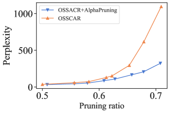
Figure 16: Using AlphaPruning to determine layerwise sparsity for OSSCAR. The $x$-axis pruning ratio represents the fraction of pruned parameters relative to the total parameters in the linear sublayer of multi-head attention and the second sublayer of the feed-forward network, any other type of sublayers are not included. The model used is OPT-6.7B, and perplexity ($\downarrow$) is evaluated on WikiText.

H.7 Mixed-Precision Quantization

We provide additional results to show that our method can enhance mixed-precision quantization by allocating precision to layers. We still use the PL_Alpha_Hill metric to estimate the heavy-tail extent of each layer, and more heavy-tailed layers are then allocated with higher precision.

Table 20 shows that, compared to three baselines (random assignment, assigned by the norm of weights, and OWL), our AlphaPruning method can always achieve the lowest perplexity under three types of mixed-precision quantization. Our experimental setup follows Tang et al. (2022).

Method	Mixed 3/4 Bit	Mixed 2/3/4 Bit	Mixed 2/4 Bit
Random	12.04	11455.54	14817.12
$L1$ norm	14.61	13959.42	33679.21
OWL	9.54	311.95	8429.39
Ours	9.01	261.39	7630.14

Table 20: Perplexity ($\downarrow$) of different methods on allocating precision to different layers for mixed-precision quantization with LLaMA-7B on WikiText.

H.8 More fine-tuning results

Here, we provide results for LoRA fine-tuning pruned LLaMA-7B with a sparsity of 70% using SparseGPT. We compare AlphaPruning with Uniform and OWL. The experiment settings align with Section 5.3. Table 21 summarizes the results for perplexity and mean zero-shot accuracies after fine-tuning pruned LLaMA-7B models, which show that the performance improvement achieved by our method doesn’t diminish after fine-tuning.

Method	Sparsity	Fine-tuning	Perplexity ($\downarrow$)	Zero-shot accuracy ($\uparrow$)
Dense model	–	2717	5.68	60.08
Uniform	70%	2717	26.30	41.52
Uniform	70%	LoRA	11.21	49.00
OWL	70%	2717	19.49	44.65
OWL	70%	LoRA	11.13	49.33
Ours	70%	2717	18.54	45.48
Ours	70%	LoRA	10.95	49.51

Table 21: WikiText validation perplexity and mean zero-shot tasks accuracy of SparseGPT pruned LLaMA-7B at 70% sparsity after LoRA fine-tuning on 30,000 C4 dataset samples.

H.9 More results on vision models

Here, we present more CV task results. We choose three widely used non-uniform layer-wise sparsity methods in the CV context including Global Frankle and Carbin (2018), ERK Mocanu et al. (2018), LAMP Lee et al. (2020). Here, we use four ImageNet-1K pre-trained models (ViT-L, ViT-B, DeiT-B, DeiT-S), and we prune them to different sparsities.

	ViT-B 16/224			ViT-L 16/224			DeiT-S 16/224			DeiT-B 16/224
Method	40%	50%	60%	40%	50%	60%	40%	50%	60%	40%	50%	60%
Uniform	70.87	59.46	29.97	76.05	68.73	39.45	75.62	68.98	50.49	80.08	76.37	61.72
Global Frankle and Carbin (2018)	66.81	45.75	8.09	75.42	65.12	29.14	74.17	65.77	38.87	79.94	75.09	57.01
ERK Mocanu et al. (2018)	70.89	60.49	33.15	76.26	69.51	40.57	75.65	69.80	52.95	80.05	76.22	63.49
LAMP Lee et al. (2020)	69.45	57.51	26.99	75.71	67.29	30.80	75.51	69.46	50.79	80.19	76.35	63.32
Ours	71.58	64.29	44.21	76.86	72.12	55.62	77.07	72.38	60.92	80.21	77.11	64.56

Table 22: ImageNet-1K Accuracy ($\uparrow$) with various layerwise sparsity using Magnitude-based pruning, without finetuning. The results are shown at 40%, 50%, and 60% sparsity on ViT-B, ViT-L, DeiT-S, and DeiT-B models. Higher accuracy is better.

H.10 Zero-shot tasks performance

For zero-shot results in Section 5.2, the 7 evaluated zero-shot tasks are: BoolQ Clark et al. (2019), RTE Wang et al. (2018), HellaSwag Zellers et al. (2019), WinoGrande Sakaguchi et al. (2021), ARC Easy and Challenge Clark et al. (2018) and OpenbookQA Mihaylov et al. (2018). We show the task-wise performance in Table 23 and Table 24.

Appendix I Experiments Compute Resources

We conducted all our experiments using NVIDIA L40 (40GB) GPUs. Specifically, we used a single NVIDIA L40 GPU for pruning the 7B and 13B models, 4 GPUs for the 30B models, and 8 GPUs for the 65B models. For the LoRA fine-tuning, we operated under a constrained computational budget, employing 2x 40GB GPUs for the 7B models. Detailed information on the computational complexity of AlphaPruning is provided in Appendix H.4.

Model	Method	BoolQ	RTE	HellaSwag	WinoGrande	ARC-e	ARC-c	OBQA	Mean
	Dense	75.02	66.79	56.94	70.00	75.29	41.89	34.60	60.08
	Magnitude	38.29	52.71	26.65	51.38	26.68	19.80	11.60	32.30
	OWL $w$. Magnitude	37.86	52.71	27.32	52.57	28.96	22.01	13.60	33.57
Llama-V1	Ours $w$. Magnitude	40.31	53.69	30.87	51.22	36.24	21.76	16.20	35.67
7B	Wanda	56.45	55.96	28.94	51.38	33.32	18.26	13.80	36.73
	OWL $w$. Wanda	62.63	58.84	34.89	58.64	46.97	24.32	17.60	43.41
	Ours $w$. Wanda	66.12	59.93	36.26	62.35	43.90	25.17	17.20	44.42
	SparseGPT	64.65	53.69	33.73	56.59	42.93	22.10	17.60	41.52
	OWL $w$. SparseGPT	66.15	52.71	37.08	62.35	48.40	26.02	19.80	44.65
	Ours $w.$ SparseGPT	68.26	55.96	37.81	64.01	46.17	27.39	18.80	45.48
	Dense	77.86	70.75	59.91	72.61	77.40	46.42	33.20	62.59
	Magnitude	52.97	50.54	26.58	50.75	28.45	20.56	14.80	34.95
	OWL $w$. Magnitude	55.75	49.10	27.80	50.28	31.23	23.89	20.00	36.86
Llama-V1	Ours $w$. Magnitude	61.28	46.93	30.24	50.43	31.23	26.28	21.20	38.23
13B	Wanda	61.90	52.71	30.50	53.12	40.91	17.58	15.60	38.90
	OWL $w$. Wanda	62.81	52.71	38.57	63.46	57.07	26.37	20.40	45.91
	Ours $w$. Wanda	64.83	52.71	41.04	64.96	59.39	28.24	21.20	47.48
	SparseGPT	66.76	52.70	37.08	63.06	53.07	26.02	21.00	45.67
	OWL $w.$ Sparsegpt	66.82	53.07	40.36	66.22	57.37	28.67	20.80	47.61
	Ours $w.$ Sparsegpt	67.58	54.51	42.43	67.80	55.47	29.10	22.00	48.41
	Dense	82.69	67.15	63.35	75.77	80.43	52.90	36.00	65.47
	Magnitude	39.30	46.21	25.77	52.49	25.29	21.50	16.20	32.39
	OWL $w$. Magnitude	39.93	58.48	25.94	52.88	27.31	18.60	14.00	33.88
Llama-V1	Ours $w$. Magnitude	62.02	47.29	32.61	57.14	47.18	27.47	24.20	42.56
30B	Wanda	66.09	56.68	43.96	67.09	65.28	31.83	26.60	51.07
	OWL $w$. Wanda	65.02	49.46	47.69	69.77	68.98	36.62	29.20	52.38
	Ours $w$. Wanda	63.82	58.12	49.40	71.27	69.40	38.31	31.00	54.48
	SparseGPT	68.13	61.01	44.50	68.75	65.70	33.53	27.60	52.75
	OWL $w.$ SparseGPT	67.95	55.60	46.96	72.22	67.13	35.49	26.80	53.16
	Ours $w.$ SparseGPT	68.96	57.04	47.49	72.30	67.97	34.73	30.00	54.07
	Dense	84.60	69.68	65.40	77.51	80.95	52.82	38.40	67.05
	Magnitude	51.85	54.51	38.55	56.67	57.35	29.95	26.40	45.04
	OWL $w$. Magnitude	70.30	52.71	50.01	67.88	65.40	35.75	31.80	53.42
Llama-V1	Ours $w$. Magnitude	70.65	62.45	51.35	66.61	66.50	37.54	31.40	55.22
65B	Wanda	76.45	56.68	47.50	69.61	70.55	35.92	27.60	54.90
	OWL $w$. Wanda	78.50	58.48	50.90	74.11	70.70	38.05	30.60	57.34
	Ours $w$. Wanda	81.85	61.01	52.55	75.06	71.60	40.02	30.40	58.93
	SparseGPT	81.00	58.84	50.70	74.66	70.90	40.19	28.40	57.81
	OWL $w.$ SparseGPT	81.30	67.15	51.25	74.98	68.35	37.71	27.00	58.25
	Ours $w.$ SparseGPT	83.80	71.48	52.40	74.59	69.30	38.05	38.05	59.72

Table 23: Accuracies (%) of LLaMA for 7 zero-shot tasks with unstructured 70% sparsity. We compare AlphaPruning with uniform pruning ratios and OWL using Magnitude-based pruning, Wanda and SparseGPT.

Model	Method	BoolQ	RTE	HellaSwag	WinoGrande	ARC-e	ARC-c	OBQA	Mean
	Dense	62.81	59.71	77.73	69.14	76.30	43.43	31.40	59.71
	Magnitude	37.95	53.07	25.96	49.25	27.74	22.70	17.00	33.38
	OWL $w$. Magnitude	38.75	52.35	27.38	48.38	32.28	22.27	17.80	34.17
Llama-V2	Ours $w$. Magnitude	57.43	51.99	28.03	51.14	31.99	23.81	20.60	37.86
7B	Wanda	50.64	52.71	27.80	50.04	30.64	18.60	12.20	34.66
	OWL $w$. Wanda	62.11	52.71	31.83	55.96	43.52	20.31	16.80	40.46
	Ours $w$. Wanda	62.23	52.71	34.56	60.85	43.27	22.27	18.00	41.98
	SparseGPT	65.38	53.43	33.55	57.62	44.52	22.91	16.40	41.84
	OWL $w.$ SparseGPT	66.94	52.71	36.57	63.06	49.33	24.49	21.60	44.96
	Ours $w.$ SparseGPT	65.93	54.15	36.83	62.19	49.62	24.23	19.80	44.68
	Dense	80.61	65.34	60.04	72.22	79.46	48.46	35.20	63.05
	Magnitude	38.72	52.70	27.56	49.33	31.27	20.73	14.60	33.56
	OWL $w$. Magnitude	38.69	52.71	34.59	54.30	38.97	23.81	15.80	36.98
Llama-V2	Ours $w$. Magnitude	70.55	52.71	37.13	62.98	42.51	27.22	18.60	44.53
13B	Wanda	62.39	52.71	28.98	51.14	35.10	18.00	11.80	37.16
	OWL $w$. Wanda	63.46	52.71	36.31	60.46	55.64	24.91	21.80	45.04
	Ours $w$. Wanda	62.57	54.87	40.28	67.32	54.46	29.35	21.60	47.21
	SparseGPT	66.64	52.71	36.26	59.91	54.00	25.85	20.80	45.17
	OWL $w.$ SparseGPT	68.04	54.15	39.31	65.75	57.70	27.82	22.80	47.94
	Ours $w.$ SparseGPT	68.13	57.04	41.26	68.03	57.15	29.18	24.00	49.26
	Dense	83.50	67.87	66.00	77.98	82.60	54.27	37.20	67.06
	Magnitude	39.15	54.51	42.55	57.22	56.35	31.57	24.20	43.65
	OWL $w$. Magnitude	64.45	53.51	45.45	68.06	61.00	33.98	27.00	50.49
Llama-V2	Ours $w$. Magnitude	63.10	53.07	45.65	67.09	62.55	33.96	29.60	50.72
70B	Wanda	74.30	60.65	49.10	74.43	71.85	38.74	28.00	56.72
	Ours $w$. Wanda	73.65	63.18	51.40	74.74	72.70	38.13	29.60	57.63
	SparseGPT	80.75	63.90	52.30	75.77	73.60	41.64	29.80	59.68
	OWL $w.$ SparseGPT	79.25	64.26	51.95	74.98	73.00	40.53	30.40	59.20
	Ours $w.$ SparseGPT	80.40	70.04	51.90	75.06	74.10	40.87	29.20	60.23

Table 24: Accuracies (%) of LLaMA-2 for 7 zero-shot tasks with unstructured 70% sparsity. We compare AlphaPruning with uniform pruning ratios and OWL using Magnitude-based pruning, Wanda, and SparseGPT.

References

- Alstott et al. (2014) Jeff Alstott, Ed Bullmore, and Dietmar Plenz. powerlaw: a python package for analysis of heavy-tailed distributions. PloS one, 9(1):e85777, 2014.
- Barsbey et al. (2021) Melih Barsbey, Milad Sefidgaran, Murat A Erdogdu, Gael Richard, and Umut Simsekli. Heavy tails in sgd and compressibility of overparametrized neural networks. Advances in neural information processing systems, 34:29364–29378, 2021.
- Bhojanapalli et al. (2021) Srinadh Bhojanapalli, Ayan Chakrabarti, Andreas Veit, Michal Lukasik, Himanshu Jain, Frederick Liu, Yin-Wen Chang, and Sanjiv Kumar. Leveraging redundancy in attention with reuse transformers. Technical Report Preprint: arXiv:2110.06821, 2021.
- Blalock et al. (2020) Davis Blalock, Jose Javier Gonzalez Ortiz, Jonathan Frankle, and John Guttag. What is the state of neural network pruning? Proceedings of Machine Learning and Systems, 2:129–146, 2020.
- Brown et al. (2020) Tom Brown, Benjamin Mann, Nick Ryder, Melanie Subbiah, Jared D Kaplan, Prafulla Dhariwal, Arvind Neelakantan, Pranav Shyam, Girish Sastry, Amanda Askell, et al. Language models are few-shot learners. Advances in Neural Information Processing Systems, 33:1877–1901, 2020.
- Clark et al. (2019) Christopher Clark, Kenton Lee, Ming-Wei Chang, Tom Kwiatkowski, Michael Collins, and Kristina Toutanova. Boolq: Exploring the surprising difficulty of natural yes/no questions. Technical Report Preprint: arXiv:1905.10044, 2019.
- Clark et al. (2018) Peter Clark, Isaac Cowhey, Oren Etzioni, Tushar Khot, Ashish Sabharwal, Carissa Schoenick, and Oyvind Tafjord. Think you have solved question answering? try arc, the ai2 reasoning challenge. Technical Report Preprint: arXiv:1803.05457, 2018.
- Clauset et al. (2009) Aaron Clauset, Cosma Rohilla Shalizi, and Mark EJ Newman. Power-law distributions in empirical data. SIAM review, 51(4):661–703, 2009.
- Couillet and Liao (2022) Romain Couillet and Zhenyu Liao. Random Matrix Methods for Machine Learning. Cambridge University Press, 2022.
- Dettmers et al. (2022) Tim Dettmers, Mike Lewis, Younes Belkada, and Luke Zettlemoyer. Llm. int8 (): 8-bit matrix multiplication for transformers at scale. Technical Report Preprint: arXiv:2208.07339, 2022.
- Dong et al. (2019) Zhen Dong, Zhewei Yao, Amir Gholami, Michael W Mahoney, and Kurt Keutzer. Hawq: Hessian aware quantization of neural networks with mixed-precision. In Proceedings of the IEEE/CVF International Conference on Computer Vision, pages 293–302, 2019.
- Dosovitskiy et al. (2020) Alexey Dosovitskiy, Lucas Beyer, Alexander Kolesnikov, Dirk Weissenborn, Xiaohua Zhai, Thomas Unterthiner, Mostafa Dehghani, Matthias Minderer, Georg Heigold, Sylvain Gelly, et al. An image is worth 16x16 words: Transformers for image recognition at scale. Technical Report Preprint: arXiv:2010.11929, 2020.
- El Halabi et al. (2022) Marwa El Halabi, Suraj Srinivas, and Simon Lacoste-Julien. Data-efficient structured pruning via submodular optimization. Advances in Neural Information Processing Systems, 35:36613–36626, 2022.
- Evci et al. (2020) Utku Evci, Trevor Gale, Jacob Menick, Pablo Samuel Castro, and Erich Elsen. Rigging the lottery: Making all tickets winners. In International Conference on Machine Learning (ICML), pages 2943–2952, 2020.
- Frankle and Carbin (2018) Jonathan Frankle and Michael Carbin. The lottery ticket hypothesis: Finding sparse, trainable neural networks. Technical Report Preprint: arXiv:1803.03635, 2018.
- Frantar and Alistarh (2023a) Elias Frantar and Dan Alistarh. Massive language models can be accurately pruned in one-shot. Technical Report Preprint: arXiv:2301.00774, 2023a.
- Frantar and Alistarh (2023b) Elias Frantar and Dan Alistarh. Sparsegpt: Massive language models can be accurately pruned in one-shot. In International Conference on Machine Learning, pages 10323–10337, 2023b.
- Gale et al. (2019) Trevor Gale, Erich Elsen, and Sara Hooker. The state of sparsity in deep neural networks. Technical Report Preprint: arXiv:1902.09574, 2019.
- Gale et al. (2020) Trevor Gale, Matei Zaharia, Cliff Young, and Erich Elsen. Sparse gpu kernels for deep learning. In SC20: International Conference for High Performance Computing, Networking, Storage and Analysis, pages 1–14. IEEE, 2020.
- Gao et al. (2023) Leo Gao, Jonathan Tow, Baber Abbasi, Stella Biderman, Sid Black, Anthony DiPofi, Charles Foster, Laurence Golding, Jeffrey Hsu, Alain Le Noac’h, Haonan Li, Kyle McDonell, Niklas Muennighoff, Chris Ociepa, Jason Phang, Laria Reynolds, Hailey Schoelkopf, Aviya Skowron, Lintang Sutawika, Eric Tang, Anish Thite, Ben Wang, Kevin Wang, and Andy Zou. A framework for few-shot language model evaluation, 12 2023.
- Gromov et al. (2024) Andrey Gromov, Kushal Tirumala, Hassan Shapourian, Paolo Glorioso, and Daniel A Roberts. The unreasonable ineffectiveness of the deeper layers. arXiv preprint arXiv:2403.17887, 2024.
- Han et al. (2015) Song Han, Jeff Pool, John Tran, and William Dally. Learning both weights and connections for efficient neural network. In Advances in Neural Information Processing Systems, pages 1135–1143, 2015.
- Hill (1975) Bruce M Hill. A simple general approach to inference about the tail of a distribution. The annals of statistics, pages 1163–1174, 1975.
- Hu et al. (2021) Edward J Hu, Yelong Shen, Phillip Wallis, Zeyuan Allen-Zhu, Yuanzhi Li, Shean Wang, Lu Wang, and Weizhu Chen. Lora: Low-rank adaptation of large language models. Technical Report Preprint: arXiv:2106.09685, 2021.
- Jaiswal et al. (2023) Ajay Jaiswal, Shiwei Liu, Tianlong Chen, and Zhangyang Wang. The emergence of essential sparsity in large pre-trained models: The weights that matter. Technical Report Preprint: arXiv:2306.03805, 2023.
- Janowsky (1989) Steven A Janowsky. Pruning versus clipping in neural networks. Physical Review A, 39(12):6600, 1989.
- Jiang et al. (2023) Albert Q Jiang, Alexandre Sablayrolles, Arthur Mensch, Chris Bamford, Devendra Singh Chaplot, Diego de las Casas, Florian Bressand, Gianna Lengyel, Guillaume Lample, Lucile Saulnier, et al. Mistral 7b. (Preprint: arXiv:2310.06825), 2023.
- Kim et al. (2023) Sehoon Kim, Coleman Hooper, Amir Gholami, Zhen Dong, Xiuyu Li, Sheng Shen, Michael W Mahoney, and Kurt Keutzer. Squeezellm: Dense-and-sparse quantization. Technical Report Preprint: arXiv:2306.07629, 2023.
- Kothapalli et al. (2024) Vignesh Kothapalli, Tianyu Pang, Shenyang Deng, Zongmin Liu, and Yaoqing Yang. Crafting heavy-tails in weight matrix spectrum without gradient noise. arXiv preprint arXiv:2406.04657, 2024.
- Kovaleva et al. (2021) Olga Kovaleva, Saurabh Kulshreshtha, Anna Rogers, and Anna Rumshisky. Bert busters: Outlier dimensions that disrupt transformers. Technical Report Preprint: arXiv:2105.06990, 2021.
- Kurtic et al. (2022) Eldar Kurtic, Daniel Campos, Tuan Nguyen, Elias Frantar, Mark Kurtz, Benjamin Fineran, Michael Goin, and Dan Alistarh. The optimal bert surgeon: Scalable and accurate second-order pruning for large language models. Technical Report Preprint: arXiv:2203.07259, 2022.
- Kurtic et al. (2023) Eldar Kurtic, Denis Kuznedelev, Elias Frantar, Michael Goin, and Dan Alistarh. Sparse fine-tuning for inference acceleration of large language models, 2023. URL https://arxiv.org/abs/2310.06927.
- Kuzmin et al. (2019) Andrey Kuzmin, Markus Nagel, Saurabh Pitre, Sandeep Pendyam, Tijmen Blankevoort, and Max Welling. Taxonomy and evaluation of structured compression of convolutional neural networks. arXiv preprint arXiv:1912.09802, 2019.
- Landau et al. (2023) Itamar D Landau, Gabriel C Mel, and Surya Ganguli. Singular vectors of sums of rectangular random matrices and optimal estimation of high-rank signals: The extensive spike model. Physical Review E, 108(5):054129, 2023.
- LeCun et al. (1990) Yann LeCun, John S Denker, and Sara A Solla. Optimal brain damage. In Advances in Neural Information Processing Systems, pages 598–605, 1990.
- Lee et al. (2020) Jaeho Lee, Sejun Park, Sangwoo Mo, Sungsoo Ahn, and Jinwoo Shin. Layer-adaptive sparsity for the magnitude-based pruning. Technical Report Preprint arXiv:2010.07611, 2020.
- Lin et al. (2020) Mingbao Lin, Rongrong Ji, Yuxin Zhang, Baochang Zhang, Yongjian Wu, and Yonghong Tian. Channel pruning via automatic structure search. Technical Report Preprint: arXiv:2001.08565, 2020.
- Liu et al. (2022a) Shiwei Liu, Tianlong Chen, Xiaohan Chen, Li Shen, Decebal Constantin Mocanu, Zhangyang Wang, and Mykola Pechenizkiy. The unreasonable effectiveness of random pruning: Return of the most naive baseline for sparse training. Technical Report Preprint: arXiv:2202.02643, 2022a.
- Liu et al. (2022b) Zhuang Liu, Hanzi Mao, Chao-Yuan Wu, Christoph Feichtenhofer, Trevor Darrell, and Saining Xie. A convnet for the 2020s. In Proceedings of the IEEE/CVF conference on computer vision and pattern recognition, pages 11976–11986, 2022b.
- Ma et al. (2023) Xinyin Ma, Gongfan Fang, and Xinchao Wang. Llm-pruner: On the structural pruning of large language models. Technical Report Preprint: arXiv:2305.11627, 2023.
- Martin and Mahoney (2017) Charles H Martin and Michael W Mahoney. Rethinking generalization requires revisiting old ideas: statistical mechanics approaches and complex learning behavior. Technical Report Preprint: arXiv:1710.09553, 2017.
- Martin and Mahoney (2019) Charles H Martin and Michael W Mahoney. Traditional and heavy tailed self regularization in neural network models. In International Conference on Machine Learning, 2019.
- Martin and Mahoney (2020) Charles H Martin and Michael W Mahoney. Heavy-tailed universality predicts trends in test accuracies for very large pre-trained deep neural networks. In SIAM International Conference on Data Mining, 2020.
- Martin and Mahoney (2021a) Charles H Martin and Michael W Mahoney. Post-mortem on a deep learning contest: a Simpson’s paradox and the complementary roles of scale metrics versus shape metrics. (Preprint: arXiv:2106.00734), 2021a.
- Martin and Mahoney (2021b) Charles H Martin and Michael W Mahoney. Implicit self-regularization in deep neural networks: Evidence from random matrix theory and implications for learning. Journal of Machine Learning Research, 22(165):1–73, 2021b.
- Martin et al. (2021) Charles H Martin, Tongsu Serena Peng, and Michael W Mahoney. Predicting trends in the quality of state-of-the-art neural networks without access to training or testing data. Nature Communications, 12(1):1–13, 2021.
- Men et al. (2024) Xin Men, Mingyu Xu, Qingyu Zhang, Bingning Wang, Hongyu Lin, Yaojie Lu, Xianpei Han, and Weipeng Chen. Shortgpt: Layers in large language models are more redundant than you expect. arXiv preprint arXiv:2403.03853, 2024.
- Meng et al. (2024) Xiang Meng, Shibal Ibrahim, Kayhan Behdin, Hussein Hazimeh, Natalia Ponomareva, and Rahul Mazumder. Osscar: One-shot structured pruning in vision and language models with combinatorial optimization. arXiv preprint arXiv:2403.12983, 2024.
- Merity et al. (2016) Stephen Merity, Caiming Xiong, James Bradbury, and Richard Socher. Pointer sentinel mixture models. Technical Report Preprint: arXiv:1609.07843, 2016.
- Mihaylov et al. (2018) Todor Mihaylov, Peter Clark, Tushar Khot, and Ashish Sabharwal. Can a suit of armor conduct electricity? a new dataset for open book question answering. Technical Report Preprint: arXiv:1809.02789, 2018.
- Mocanu et al. (2018) Decebal Constantin Mocanu, Elena Mocanu, Peter Stone, Phuong H Nguyen, Madeleine Gibescu, and Antonio Liotta. Scalable training of artificial neural networks with adaptive sparse connectivity inspired by network science. Nature communications, 9(1):2383, 2018.
- Mozer and Smolensky (1988) Michael C Mozer and Paul Smolensky. Skeletonization: A technique for trimming the fat from a network via relevance assessment. Advances in Neural Information Processing Systems, 1, 1988.
- NeuralMagic (2021) NeuralMagic. Neuralmagic deepsparse inference engine. 2021. URL https://github.com/neuralmagic/deepsparse.
- Puccetti et al. (2022) Giovanni Puccetti, Anna Rogers, Aleksandr Drozd, and Felice Dell’Orletta. Outliers dimensions that disrupt transformers are driven by frequency. Technical Report Preprint: arXiv:2205.11380, 2022.
- Raffel et al. (2020) Colin Raffel, Noam Shazeer, Adam Roberts, Katherine Lee, Sharan Narang, Michael Matena, Yanqi Zhou, Wei Li, and Peter J Liu. Exploring the limits of transfer learning with a unified text-to-text transformer. The Journal of Machine Learning Research, 21(1):5485–5551, 2020.
- Sakaguchi et al. (2021) Keisuke Sakaguchi, Ronan Le Bras, Chandra Bhagavatula, and Yejin Choi. Winogrande: An adversarial winograd schema challenge at scale. Communications of the ACM, 64(9):99–106, 2021.
- Sanh et al. (2020) Victor Sanh, Thomas Wolf, and Alexander M Rush. Movement pruning: Adaptive sparsity by fine-tuning. Technical Report Preprint: arXiv:2005.07683, 2020.
- Shen et al. (2020) Sheng Shen, Zhen Dong, Jiayu Ye, Linjian Ma, Zhewei Yao, Amir Gholami, Michael W Mahoney, and Kurt Keutzer. Q-bert: Hessian based ultra low precision quantization of bert. In Proceedings of the AAAI Conference on Artificial Intelligence, volume 34, pages 8815–8821, 2020.
- Sun et al. (2023) Mingjie Sun, Zhuang Liu, Anna Bair, and J Zico Kolter. A simple and effective pruning approach for large language models. Technical Report Preprint: arXiv:2306.11695, 2023.
- Sun et al. (2021) Wei Sun, Aojun Zhou, Sander Stuijk, Rob Wijnhoven, Andrew O Nelson, Henk Corporaal, et al. Dominosearch: Find layer-wise fine-grained n: M sparse schemes from dense neural networks. Advances in Neural Information Processing Systems, 34:20721–20732, 2021.
- Tang et al. (2022) Chen Tang, Kai Ouyang, Zhi Wang, Yifei Zhu, Wen Ji, Yaowei Wang, and Wenwu Zhu. Mixed-precision neural network quantization via learned layer-wise importance. In European Conference on Computer Vision, pages 259–275. Springer, 2022.
- Touvron et al. (2023a) Hugo Touvron, Thibaut Lavril, Gautier Izacard, Xavier Martinet, Marie-Anne Lachaux, Timothée Lacroix, Baptiste Rozière, Naman Goyal, Eric Hambro, Faisal Azhar, et al. Llama: Open and efficient foundation language models. Technical Report Preprint: arXiv:2302.13971, 2023a.
- Touvron et al. (2023b) Hugo Touvron, Louis Martin, Kevin Stone, Peter Albert, Amjad Almahairi, Yasmine Babaei, Nikolay Bashlykov, Soumya Batra, Prajjwal Bhargava, Shruti Bhosale, et al. Llama 2: Open foundation and fine-tuned chat models. Technical Report Preprint: arXiv:2307.09288, 2023b.
- Wang et al. (2018) Alex Wang, Amanpreet Singh, Julian Michael, Felix Hill, Omer Levy, and Samuel R Bowman. Glue: A multi-task benchmark and analysis platform for natural language understanding. Technical Report Preprint: arXiv:1804.07461, 2018.
- Wang and Tu (2020) Wenxuan Wang and Zhaopeng Tu. Rethinking the value of transformer components. Technical Report Preprint: arXiv:2011.03803, 2020.
- Wang et al. (2024) Zhichao Wang, Andrew Engel, Anand D Sarwate, Ioana Dumitriu, and Tony Chiang. Spectral evolution and invariance in linear-width neural networks. Advances in Neural Information Processing Systems, 36, 2024.
- Wen et al. (2017) Wei Wen, Cong Xu, Chunpeng Wu, Yandan Wang, Yiran Chen, and Hai Li. Coordinating filters for faster deep neural networks. In Proceedings of the IEEE international conference on computer vision, pages 658–666, 2017.
- Xia et al. (2023) Haojun Xia, Zhen Zheng, Yuchao Li, Donglin Zhuang, Zhongzhu Zhou, Xiafei Qiu, Yong Li, Wei Lin, and Shuaiwen Leon Song. Flash-llm: Enabling cost-effective and highly-efficient large generative model inference with unstructured sparsity. arXiv preprint arXiv:2309.10285, 2023.
- Xiao et al. (2023a) Guangxuan Xiao, Ji Lin, Mickael Seznec, Hao Wu, Julien Demouth, and Song Han. Smoothquant: Accurate and efficient post-training quantization for large language models. In International Conference on Machine Learning, pages 38087–38099, 2023a.
- Xiao et al. (2023b) Xuanzhe Xiao, Zeng Li, Chuanlong Xie, and Fengwei Zhou. Heavy-tailed regularization of weight matrices in deep neural networks. Technical Report Preprint: arXiv:2304.02911, 2023b.
- Xu et al. (2019) Yuhui Xu, Yuxi Li, Shuai Zhang, Wei Wen, Botao Wang, Wenrui Dai, Yingyong Qi, Yiran Chen, Weiyao Lin, and Hongkai Xiong. Trained rank pruning for efficient deep neural networks. In 2019 Fifth Workshop on Energy Efficient Machine Learning and Cognitive Computing-NeurIPS Edition (EMC2-NIPS), pages 14–17. IEEE, 2019.
- Yang et al. (2023) Yaoqing Yang, Ryan Theisen, Liam Hodgkinson, Joseph E Gonzalez, Kannan Ramchandran, Charles H Martin, and Michael W Mahoney. Test accuracy vs. generalization gap: Model selection in nlp without accessing training or testing data. In Proceedings of the ACM SIGKDD Conference on Knowledge Discovery and Data Mining, pages 3011–3021, 2023.
- Ye et al. (2020) Mao Ye, Chengyue Gong, Lizhen Nie, Denny Zhou, Adam Klivans, and Qiang Liu. Good subnetworks provably exist: Pruning via greedy forward selection. In International Conference on Machine Learning, pages 10820–10830. PMLR, 2020.
- Yin et al. (2023) Lu Yin, You Wu, Zhenyu Zhang, Cheng-Yu Hsieh, Yaqing Wang, Yiling Jia, Mykola Pechenizkiy, Yi Liang, Zhangyang Wang, and Shiwei Liu. Outlier weighed layerwise sparsity (owl): A missing secret sauce for pruning llms to high sparsity. Technical Report Preprint: arXiv:2310.05175, 2023.
- Yoshida and Miyato (2017) Yuichi Yoshida and Takeru Miyato. Spectral norm regularization for improving the generalizability of deep learning. arXiv preprint arXiv:1705.10941, 2017.
- Zellers et al. (2019) Rowan Zellers, Ari Holtzman, Yonatan Bisk, Ali Farhadi, and Yejin Choi. Hellaswag: Can a machine really finish your sentence? Technical Report Preprint: arXiv:1905.07830, 2019.
- Zhang et al. (2023) Susan Zhang, Stephen Roller, Naman Goyal, Mikel Artetxe, Moya Chen, Shuohui Chen, Christopher Dewan, Mona Diab, Xian Li, Xi Victoria Lin, et al. Opt: Open pre-trained transformer language models, 2022. (Preprint: arXiv:2205.01068), 2023.
- Zhang et al. (2015) Xiangyu Zhang, Jianhua Zou, Kaiming He, and Jian Sun. Accelerating very deep convolutional networks for classification and detection. IEEE transactions on pattern analysis and machine intelligence, 38(10):1943–1955, 2015.
- Zheng et al. (2024) Lianmin Zheng, Wei-Lin Chiang, Ying Sheng, Siyuan Zhuang, Zhanghao Wu, Yonghao Zhuang, Zi Lin, Zhuohan Li, Dacheng Li, Eric Xing, et al. Judging llm-as-a-judge with mt-bench and chatbot arena. Advances in Neural Information Processing Systems, 36, 2024.
- Zhou et al. (2023) Yefan Zhou, Tianyu Pang, Keqin Liu, Charles H. Martin, Michael W. Mahoney, and Yaoqing Yang. Temperature balancing, layer-wise weight analysis, and neural network training. In Advances in Neural Information Processing Systems, 2023.
- Zhu and Gupta (2017) Michael Zhu and Suyog Gupta. To prune, or not to prune: exploring the efficacy of pruning for model compression. Technical Report Preprint: arXiv:1710.01878, 2017.
- Zhuang et al. (2018) Zhuangwei Zhuang, Mingkui Tan, Bohan Zhuang, Jing Liu, Yong Guo, Qingyao Wu, Junzhou Huang, and Jinhui Zhu. Discrimination-aware channel pruning for deep neural networks. Advances in neural information processing systems, 31, 2018.