Online Client Scheduling and Resource Allocation for Efficient Federated Edge Learning

Zhidong Gao,  Zhenxiao Zhang,  Yu Zhang,  Tongnian Wang,  Yanmin Gong,  and Yuanxiong Guo Z. Zhang, Z. Gao, Y. Zhang, and Y. Gong are with the Department of Electrical and Computer Engineering, The University of Texas at San Antonio, San Antonio, TX, 78249. T. Wang and Y. Guo are with the Department of Information Systems and Cyber Security, The University of Texas at San Antonio, San Antonio, TX, 78249. E-mail: {zhidong.gao@my., zhenxiao.zhang@my., yu.zhang@my., tongnian.wang@my., yanmin.gong@, yuanxiong.guo@}utsa.edu
Abstract

Federated learning (FL) enables edge devices to collaboratively train a machine learning model without sharing their raw data. Due to its privacy-protecting benefits, FL has been deployed in many real-world applications. However, deploying FL over mobile edge networks with constrained resources such as power, bandwidth, and computation suffers from high training latency and low model accuracy, particularly under data and system heterogeneity. In this paper, we investigate the optimal client scheduling and resource allocation for FL over mobile edge networks under resource constraints and uncertainty to minimize the training latency while maintaining the model accuracy. Specifically, we first analyze the impact of client sampling on model convergence in FL and formulate a stochastic optimization problem that captures the trade-off between the running time and model performance under heterogeneous and uncertain system resources. To solve the formulated problem, we further develop an online control scheme based on Lyapunov-based optimization for client sampling and resource allocation without requiring the knowledge of future dynamics in the FL system. Extensive experimental results demonstrate that the proposed scheme can improve both the training latency and resource efficiency compared with the existing schemes.

Index Terms:
Federated learning, energy efficiency, latency, Lyapunov optimization, resource allocation, client sampling.

I Introduction

Edge devices, such as mobile phones, smartwatches, and drones, are being increasingly adopted in our daily life and across a wide range of industries. They generate huge amounts of data at the network edge, which need to be processed in a timely fashion to enable real-time decision-making. The traditional machine learning paradigm involves transmitting data over a network to a central cloud server for processing, resulting in significant latency, communication overhead, and privacy issues. Federated learning (FL) is an emerging learning paradigm that enables multiple agents to collaboratively learn from their respective data under the orchestration of a server without sharing their raw data [1].

Deploying FL at the mobile edge is particularly challenging due to system heterogeneity. Note that edge devices usually have different hardware resources (e.g., CPU frequency, memory, storage capacity, and battery level) and operate under different communication environments. This results in different processing delays for edge devices in the local updating stage. Since the server has to wait for all participating devices to finish the local updating before proceeding to the next round, the total training speed is constrained by the slowest device.

Meanwhile, FL faces challenges in data heterogeneity where non-IID data distribution across devices hinders the convergence behavior and can even lead to divergence under the highly heterogeneous case [2]. The challenges become more significant when data heterogeneity and system heterogeneity co-exist. For instance, when a device has little battery energy or a bad network connection, it cannot participate in the training even if its data is vital to training a satisfactory model. In this case, it is helpful for these devices to strategically plan their engagement in the learning process to conserve energy and improve the total learning efficiency.

Some prior studies have investigated the impact of system heterogeneity aiming to improve communication, computation, and energy efficiency in FL [3, 4, 5, 6]. However, these research works did not consider the potential variability of resources (e.g., battery level and data rate) at edge devices and mainly follow a uniform random sampling process to select edge devices as described in the classic FedAvg algorithm [1]. Hence, the stragglers who possess fewer resources or have a bad communication environment are chosen with the same likelihood as other devices, leading to slow training speed. Another line of research in FL aims to mitigate the impact of data heterogeneity. They either design updating rules based on sample quantities to address the data imbalance issue [7, 8] or develop adaptive FL updating algorithms  [9, 10] to address the diverging model update directions caused by different data distributions. However, fewer works have jointly considered the negative impacts of data and system heterogeneity.

In this paper, we propose a novel Lyapunov-based Resource-efficient Online Algorithm (LROA) for FL over the mobile edges. It strategically selects the participating edge devices at the beginning of each communication round based on their available hardware resources, training data sizes, and communication environments. Meanwhile, computation and communication resources are jointly optimized in each communication round. These enable FL to operate under high degrees of data and system heterogeneity, achieving higher model accuracy, lower training latency, and better resource efficiency.

Specifically, we analyze the convergence bound of the FL algorithm with arbitrary client sampling under data and system heterogeneity. Based on the convergence bound, we formulate a stochastic optimization problem that captures the trade-off between running time and model convergence under the energy constraint and uncertainty rooting from the random communication environment. The form of the optimization problem is compatible with the Lyapunov drift-plus-penalty framework. It enables us to solve the problem online without prior knowledge of system statistics. To demonstrate the effectiveness of our proposed method, we conduct experiments on two benchmark datasets, CIFAR10 and FEMNIST, under various data and system heterogeneity settings. The experimental results illustrate that our method significantly outperforms baselines in terms of the total training latency and convergence speed.

In summary, our main contributions are stated as follows:

  • We formulate a stochastic optimization problem that captures the trade-off between the running time and model convergence. Then, we design an efficient algorithm based on the Lyapunov optimization and successive upper-bound minimization (SUM) techniques to solve the problem online.

  • We conduct the convergence analysis for the FL under arbitrary client sampling and derive an error bound that reveals the impact of client sampling under assumptions of non-convex loss function and non-IID data distribution.

  • We propose LROA, a novel online resource allocation and client sampling strategy for FL with heterogeneous resources, achieving high accuracy, low latency, and high resource efficiency over mobile edge networks under uncertain environments.

  • We conduct extensive experiments on several datasets and heterogeneous settings to evaluate the effectiveness of the proposed method. The simulation result shows our method saves up to $50.1\%$ total training latency compared with baselines.

II Related works

Efficient FL implementation faces two substantial challenges: system and data heterogeneity, both capable of degrading model accuracy and increasing energy consumption and training latency [6, 11]. To overcome these challenges, most of the existing works focus on the resource aspect while ignoring client sampling in FL [12, 13, 14]. Recently, a few studies have tried to investigate the impact of client sampling with resource allocation [15, 16, 17]. However, the sampling probability of each client is assumed to be fixed across the rounds in these works, which cannot capture the dynamic changes in communication and computation resources. On the other hand, there is substantial literature to study the client sampling policy of FL solely from the learning perspective  [18, 19, 20, 21]. The key idea of these studies is to select “important” clients with higher probabilities, and the importance is determined either by their local gradient [18, 19, 20] or their local training loss [21]. These approaches work well under mild system heterogeneity. However, they may diverge or suffer from high training latency and resource cost under the high degree of system heterogeneity. As shown later in Section III-B, it is important to take both system heterogeneity and potential dynamics into account when designing the client sampling policy.

A few recent works mostly related to ours are [22][23] and [24], which also consider client sampling from both system and data heterogeneity perspectives. Specifically, Luo et al. [22] proposed an adaptive client sampling algorithm to minimize the convergence time under system and data heterogeneity. However, their analysis is restricted to the convex model and ignores the influence of communication and computation on training latency. Perazzone et al. [23] proposed a joint client sampling and power allocation scheme that minimizes the convergence bound and the average communication time under a transmit power constraint. However, they have not considered the resources consumed for local computation. Wang et al. [24] proposed an optimization problem to minimize the convergence bound under the resource constraints by adaptively determining the compressed model update and the probability of local updating. However, their resource model relies on several simplified assumptions (e.g., linear computation cost), which lack a detailed analysis for practical FL systems. Deng, et al. [25] utilizes a Lyapunov-based approach to maximize the Long-Term Average (LTA) training data size under LTA energy consumption constraint by solving a mix-integer problem. While they consider a blockchain-assisted FL system, the block mining time and energy consumption are the cores of their formulated optimization problem. Different from these studies, our goal in this paper is to minimize the total learning latency while maintaining the model accuracy by jointly optimizing the client sampling policy, communication, and computation resource allocations under both system and data heterogeneity.

III System Modeling

TABLE I: Summary of main notations.
Notation Definition
$n$ Index for device
$t$ Index for global round
$N$ Total number of devices
$M$ Model size in storage
$\bm{\theta}_{n}^{t}$ Local model of device $n$
$E$ Local epoch number
$[N]$ {1, 2, …, $N$}
$K$ Sampling frequency
$\mathcal{K}^{t}$ Set of selected devices in round $t$
$q_{n}^{t}$ Probability of client $n$ to be selected
${D}_{n}$ Local dataset size of device $n$
$w_{n}$ Local dataset fraction of device $n$
$F_{n}(\cdot)$ Local objective function of device $n$
$N_{0}$ Background noise power
$r_{n,d}$ Download rate of device $n$
$B_{n}$ Communication bandwidth of device $n$
$\bm{h}_{n}^{t}$ Channel gain between device $n$ and the server
$c_{n}$ CPU cycles per sample
$p_{n}^{t}$ Transmission power of device $n$
$\alpha_{n}$ Computing capacitance coefficient
$f_{n}^{t}$ Computing frequency of device $n$
$f_{n}^{\text{min}},f_{n}^{\text{max}}$ Minimum and maximum CPU frequency
$p_{n}^{\text{min}},p_{n}^{\text{max}}$ Minimum and maximum communication power
$\mathcal{T}_{n,u}^{t,\text{com}},\mathcal{T}_{n,d}^{t,\text{com}}$ Uploading and Downloading time
$\mathcal{E}_{n}^{t,\text{cmp}},\mathcal{E}_{n}^{t,\text{cmp}}$ Computing and communication energy
$\mathcal{T}_{n}^{t,\text{cmp}}$ Local computing time
$\mathcal{\bar{E}}_{n}$ Energy budget of device $n$
$L(t)$ Quadratic Lyapunov function
$Q_{n}^{t}$ Virtual energy consumption queue
$\Delta(t)$ One-slot conditional Lyapunov drift

III-A FL System

We consider an FL system involving $N$ edge devices (or clients) and one server. Each edge device $n\in[N]$ holds a local training dataset $\mathcal{D}_{n}=\{\xi_{n}^{i}\}_{i=1}^{D_{n}}$ where $\xi_{n}^{i}$ is a training example and $D_{n}$ is the size of the local training dataset. The total number of training examples across $N$ edge devices is $D=\sum_{n=1}^{N}D_{n}$. Additionally, we define $\ell(\bm{\theta};\xi_{n}^{i})$ as the per-sample loss function, e.g., cross-entropy or mean square error, where $\bm{\theta}\in\mathbb{R}^{d}$ denotes the model parameters. Then, the local objective of client $n$ can be expressed as

$$F_{n}(\bm{\theta})\coloneqq\frac{1}{D_{n}}\sum_{i\in\mathcal{D}_{n}}\ell(\bm{\theta};\xi_{n}^{i}).$$ (1)

Let $w_{n}=D_{n}/D$ be the data weight of $n$-th edge device such that $\sum_{n=1}^{N}w_{n}=1,0<w_{n}\leq 1$. The goal of the FL is to minimize the following global objective:

$$\min_{\bm{\theta}}F(\bm{\theta})\coloneqq\sum_{n=1}^{N}w_{n}F_{n}(\bm{\theta}).$$ (2)

III-B FL with Adaptive Resource Control and Client Sampling

The most popular algorithm to solve (2) is FedAvg [1]. Specifically, at the beginning of $t$-th FL round, the server uniformly samples a subset of edge devices $\mathcal{K}^{t}$ and broadcasts the global model $\bm{\theta}^{t}$ to the devices. Then, each edge device $n\in\mathcal{K}^{t}$ initializes the local model $\bm{\theta}_{n}^{t,0}$ by the received global model and runs $E$ epochs SGD based on its local dataset to update the local model. Next, each edge device uploads the local model $\bm{\theta}_{n}^{t,E}$ to the server, which aggregates the received local models to compute the latest global model $\bm{\theta}^{t+1}$. This process repeats multiple rounds until satisfying the convergence criteria.

One common assumption among FedAvg and its variants [2, 9] is that clients are uniformly sampled at each round. However, this assumption does not align with the practical FL systems, as the client may drop out of the training due to various reasons, e.g., network failure or congestion. Moreover, the stragglers are sampled with the same probability, which significantly prolongs the training latency. To improve the efficiency of the FL system, we propose to adopt adaptive sampling so that the stragglers are less likely to be selected during the training.

Building upon recent research [26], we assume that, in round $t$, the server forms a sampled edge device set $\mathcal{K}^{t}$ by sampling $K$ times with replacement from $N$ edge devices. Here, the sampling probability $q_{n}^{t}$ of edge device $n$ in round $t$ should satisfy the following constraints:

$$\sum_{n=1}^{N}q_{n}^{t}=1,\quad\quad q_{n}^{t}\in(0,1],~{}~{}\forall n\in[N].$$ (3)

We summarize the FL algorithm with adaptive client sampling in Algorithm 1. Specifically, we assume the server to be the coordinator for the FL system. It collects the device-specific parameters from devices, including the CPU cycle per sample $c_{n}$, the size of the training data $D_{n}$, energy budget $\mathcal{\bar{E}}_{n}$, the capacitance coefficient $\alpha_{n}$, and decision boundaries $f_{n}^{\text{min}},f_{n}^{\text{max}},p_{n}^{\text{min}},p_{n}^{\text{max}}$, before the training starts. Other input parameters are determined based on performance criteria, e.g., sampling frequency $K$ and the local epoch $E$, or observable by the server, e.g., background noise power $N_{0}$ and bandwidth $B$. At the beginning of $t$-th round, each edge device $n$ records its channel gain $h_{n}^{t}$ and transmits it to the server (line 3). Server determines the transmission power $p_{n}^{t}$, CPU frequency $f_{n}^{t}$, and sampling probability $q_{n}^{t}$ for each client by Algorithm 2 (line 4), which will be elaborated in Section VI. Then, the server chooses the set of training devices $\mathcal{K}^{t}$ by sampling $K$ times according to the probability $\{q_{n}^{t},\forall n\}$ (line 5), and broadcasts the latest global model $\bm{\theta}^{t}$ to all edge devices in $\mathcal{K}^{t}$ (line 6). Each selected edge devices $n\in\mathcal{K}^{t}$ initializes its local model $\bm{\theta}_{n}^{t,0}$ to the received global model $\bm{\theta}^{t}$ and downloads the control parameters $f_{n}^{t}$ and $p_{n}^{t}$ (line 8). Next, the selected edge devices perform $E$ epochs of SGD to update their local model $\bm{\theta}_{n}^{t,0}$ (lines 9). After that, all selected edge devices upload their local model updates $(\bm{\theta}_{n}^{t,E}-\bm{\theta}^{t})$ to the server (line 10). Finally, the server aggregates the local model updates from $\mathcal{K}^{t}$ to compute the global model $\bm{\theta}^{t+1}$ for the next round (line 12). Since the edge devices are sampled with different probabilities, we re-weight each model update using the corresponding probability and sampling times as follows:

$$\bm{\theta}^{t+1}\xleftarrow[]{}\bm{\theta}^{t}+\sum_{n\in\mathcal{K}^{t}}\frac{w_{n}}{Kq_{n}^{t}}(\bm{\theta}_{n}^{t,E}-\bm{\theta}^{t}).$$ (4)

Here (4) ensures the aggregated model is unbiased towards that with full client participation. We provide the proof in Appendix A. Note it aligns with the aggregation method employed in [22], which shares a similar client sampling scheme to ours.

Input: Sampling frequency $K$, local epoch $E$, background noise power $N_{0}$, bandwidth $B$, model size $M$, download rate $r_{n,d}$, CPU cycle per sample $c_{n},\forall n$, training data size $D_{n},\forall n$, capacitance coefficient $\alpha_{n},\forall n$, energy budget $\bar{\mathcal{E}}_{n}$, decision boundaries $f_{n}^{\text{min}},f_{n}^{\text{max}},p_{n}^{\text{min}},p_{n}^{\text{max}}$.
Output: Final learned model $\bm{\theta}^{T}$

Algorithm 1 FL with LROA
1:  Initial global model $\bm{\theta}^{0}$;
2:  for round $t=0,\ldots,T-1$ do
3:     Each edge device online observes $h_{n}^{t}$ and uploads it to the server;
4:     Server determines $\{p_{n}^{t},\forall n\},\{f_{n}^{t},\forall n\},\{{q}_{n}^{t},\forall n\}$ by Algorithm 2;
5:     Server samples $K$ times by $\{q_{n}^{t},\forall n\}$ to build $\mathcal{K}^{t}$;
6:     Server broadcasts $\bm{\theta}^{t}$ to edge devices in $\mathcal{K}^{t}$;
7:     for  edge device $n\in\mathcal{K}^{t}$ in parallel do
8:        Edge device downloads the control parameters $f_{n}^{t},p_{n}^{t}$ from the server and initializes its local model $\bm{\theta}_{n}^{t,0}\xleftarrow[]{}\bm{\theta}^{t}$;
9:        Edge device updates $\bm{\theta}_{n}^{t,0}$ with $E$ epochs to compute $\bm{\theta}_{n}^{t,E}$ under computation frequency $f_{n}^{t}$;
10:        Edge device uploads $\bm{\theta}_{n}^{t,E}-\bm{\theta}_{n}^{t,0}$ to the server with communication power $p_{n}^{t}$;
11:     end for
12:     $\bm{\theta}^{t+1}\xleftarrow[]{}\bm{\theta}^{t}+\sum_{n\in\mathcal{K}^{t}}\frac{w_{n}}{Kq_{n}^{t}}(\bm{\theta}_{n}^{t,E}-\bm{\theta}^{t})$;
13:  end for

III-C Communication Time

Without loss of generality, we assume the frequency-division multiple access (FDMA) protocol is adopted, and the server evenly allocates its communication bandwidth among all selected edge devices. Let $B$ be the total communication bandwidth of the server. Then, the allocated bandwidth for a selected edge device is $B_{n}={B}/{K},\forall n\in\mathcal{K}^{t}$, where $K$ is the number of selected edge devices at each communication round. Furthermore, we model the channel gain from edge device $n$ to the server as a discrete-time random process $h_{n}^{t}$. According to Shannon’s capacity theorem, the achievable uploading transmission rate $r_{n,u}^{t}$ of edge device $n$ at round $t$ is given by

$$\begin{split}r_{n,u}^{t}=B_{n}\log_{2}(1+\frac{h_{n}^{t}p_{n}^{t}}{N_{0}}),\quad\forall n\in\mathcal{K}^{t},\end{split}$$ (5)

where $p_{n}^{t}$ is the edge device’s transmission power, $N_{0}$ is the additive Gaussian white noise.

Consequently, the communication time for uploading $\mathcal{T}_{n,u}^{t,\text{com}}$ and downloading $\mathcal{T}_{n,d}^{t,\text{com}}$ are

$\displaystyle\mathcal{T}_{n,u}^{t,\text{com}}$ $\displaystyle=\frac{M}{r_{n,u}^{t}}=\frac{MK}{B\log_{2}(1+\frac{h_{n}^{t}p_{n}^{t}}{N_{0}})},\quad\forall n\in\mathcal{K}^{t},$ (6)
$\displaystyle\mathcal{T}_{n,d}^{t,\text{com}}$ $\displaystyle=\frac{M}{r_{n,d}},\quad\forall n\in\mathcal{K}^{t},$ (7)

where $M$ denotes the size of the model update, and $r_{n,d}$ is downloading transmission rate.

III-D Computation Time

Let $c_{n}$ denote the number of CPU cycles required to process a single data sample for edge device $n$. Then, the total number of CPU cycles required to train the local model at each round is $Ec_{n}D_{n}$. Thus, the per-round local computation time for edge device $n$ can be estimated as

$$\mathcal{T}_{n}^{t,\text{cmp}}=\frac{Ec_{n}D_{n}}{f_{n}^{t}},\quad\forall n\in\mathcal{K}^{t},$$ (8)

where $f_{n}^{t}$ is the CPU frequency that edge device $n$ used for local model updating at round $t$.

III-E Per-round Training Time

The per-round training time for a client is composed of the model downloading time, local training time, and model update uploading time. Let $\mathcal{T}_{n}^{t}$ denote the per-round time consumption of edge device $n$, then we have

$$\mathcal{T}_{n}^{t}=\mathcal{T}_{n}^{t,\text{cmp}}+\mathcal{T}_{n,u}^{t,\text{com}}+\mathcal{T}_{n,d}^{t,\text{com}},\quad\forall n\in\mathcal{K}^{t}.$$ (9)

In synchronous FL, the server computes the global model after all clients have uploaded their local model. Therefore, the slowest edge device determines the training latency of one global round

$$\mathcal{T}^{t}=\underset{n\in\mathcal{K}^{t}}{\max}\{\mathcal{T}_{n}^{t}\},$$ (10)

where $\mathcal{T}^{t}$ is the wall-clock training time of FL at round $t$.Note that directly optimizing the selected client set $\mathcal{K}^{t}$ is not feasible since the relationship between sample probabilities $q_{n}^{t}$ and the selected client set $\mathcal{K}^{t}$ is complex and hard to handle. Therefore, we adopt a similar strategy as in [22] and approximate the per-round completion time as

$$\underset{n\in\mathcal{K}^{t}}{\max}\{\mathcal{T}_{n}^{t}\}\approx\sum_{n=1}^{N}q_{n}^{t}\mathcal{T}_{n}^{t}.$$ (11)

III-F Energy Consumption

In each communication round, the selected edge devices perform $E$ epochs of local training. Following [12], the computation energy of device $n$ at round $t$ is

$$\mathcal{E}_{n}^{t,\text{cmp}}=\frac{E\alpha_{n}c_{n}D_{n}(f_{n}^{t})^{2}}{2},\quad\forall n\in\mathcal{K}^{t},$$ (12)

where $\alpha_{n}/2$ is the effective capacitance coefficient of device $n$ (determined by chip architecture).

In practice, the available CPU frequency $f_{n}^{t}$ of an edge device has an upper bound due to hardware limitations. Therefore, we have the following constraint on the CPU frequency:

$$f_{n}^{\text{min}}\leq f_{n}^{t}\leq f_{n}^{\text{max}},\quad\forall n\in\mathcal{K}^{t},$$ (13)

where $f_{n}^{\text{max}}$ and $f_{n}^{\text{min}}$ denote the maximum and minimum available CPU frequency of edge device $n$, respectively.

The communication energy of uploading for edge device $n$ at round $t$ can be estimated as

$$\mathcal{E}_{n}^{t,\text{com}}=p_{n}^{t}\mathcal{T}_{n,u}^{t,\text{com}}=\frac{p_{n}^{t}MK}{B\log_{2}(1+\frac{h_{n}^{t}p_{n}^{t}}{N_{0}})},\quad\forall n\in\mathcal{K}^{t}.$$ (14)

The energy of global model downloading is assumed to be neglectable since the receiving power of edge device is very small compared with its transmission power. Consequently, the total energy consumption of edge device $n$ at round $t$ is

$$\mathcal{E}_{n}^{t}=\mathcal{E}_{n}^{t,\text{cmp}}+\mathcal{E}_{n}^{t,\text{com}},\quad\forall n\in\mathcal{K}^{t}.$$ (15)

Since edge devices, such as mobile phones and smartwatches, are usually power-limited, and the energy consumption of edge device $n$ depends on the random channel gain $h_{n}^{t}$, we consider the following energy constraint on the time-average expected energy consumption of each edge device $n$:

$$\lim_{T\to\infty}\frac{1}{T}\sum_{t=0}^{T-1}\mathbb{E}_{h_{n}^{t}}\left[(1-(1-q_{n}^{t})^{K})\mathcal{E}_{n}^{t}\right]\leq\bar{\mathcal{E}}_{n},\quad\forall n\in[N],$$ (16)

Here $(1-(1-q_{n}^{t})^{K})$ is the likelihood of device $n$ being chosen at round $t$. Specifically, for each sampling event, the probability of a client not being selected is $1-q_{n}^{t}$. After $K$ sampling events, the compounded probability of client $n$ not being selected in any of these events is $(1-q_{n}^{t})^{K}$. Then, the probability of a client being selected at least once during $K$ times sampling is $1-(1-q_{n}^{t})^{K}$.

In practice, due to the edge device antenna limitation, we have the following constraint on the transmission power:

$$\begin{split}p_{n}^{\min}\leq p_{n}^{t}\leq p_{n}^{\max},\quad\forall n\in\mathcal{K}^{t}.\end{split}$$ (17)

where $p_{n}^{\min},p_{n}^{\max}$ denote the minimum and maximum transmission power of edge device $n$.

IV Convergence Analysis

In this section, we derive the convergence properties of Algorithm 1 under non-convex and non-IID settings. Before stating our convergence results, we make the following assumptions:

Assumption 1 (Smoothness).

Each local objective function $F_{n}:\mathbb{R}^{d}\rightarrow\mathbb{R}$ is $\beta$-smooth for all $n\in[N]$, i.e.,

$$\|\nabla F_{n}(\bm{\theta})-\nabla F_{n}(\bm{\theta}^{\prime})\|\leq\beta\|\bm{\theta}-\bm{\theta}^{\prime}\|,\;\forall\bm{\theta},\bm{\theta}^{\prime}\in\mathbb{R}^{d}.$$
Assumption 2 (Bounded gradients).

There exists a constant $G\geq 0$ such that

$$\|\nabla F_{n}(\bm{\theta})\|_{2}^{2}\leq G^{2},\forall\bm{\theta}\in\mathbb{R}^{d},n\in[N].$$
Assumption 3 (Bounded Dissimilarity).

There exist constants $\gamma^{2}\geq 1,\kappa^{2}\geq 0$ such that $\sum_{n=1}^{N}w_{n}\|\nabla F_{n}(\bm{\theta})\|^{2}\leq\gamma^{2}\|\sum_{n=1}^{N}w_{n}\nabla F_{n}(\bm{\theta})\|^{2}+\kappa^{2}$. If the data distributions across all devices are IID, then $\gamma^{2}=1$ and $\kappa^{2}=0$.

Assumptions 1 and 2 are commonly used in the FL literature, e.g., [27][28] and [18]. Assumption 3 captures the dissimilarities of local objective functions under non-IID data distribution, such as [29] and [30]. Note that some recent works [22][23] also consider arbitrary device probabilities for FL and provide convergence analyses, but they only consider convex local objectives and IID data distribution. However, deep neural networks are usually non-convex, and the data are generally non-IID over devices in FL. Thus, our analysis is more general than prior works.

We now state the convergence analysis result in the following theorem.

Theorem 1 (Convergence Result with Adaptive Sampling Probabilities).

Under Assumptions 1, 2 and 3, if the local learning rate $\eta\leq\min\{{1}/({32E^{2}\beta^{2}\gamma^{2}}),{1}/({2\sqrt{2}E\beta})\}$, then Algorithm 1 satisfies

$$\begin{split}\frac{1}{T}\sum_{t=0}^{T-1}\mathbb{E}\|\nabla F(\bm{\theta}^{t})\|^{2}\leq&\frac{4(F(\bm{\theta}^{0})-F^{*})}{\eta TE}+8\eta^{2}\beta^{2}E^{2}\kappa^{2}\\ &+\frac{2\beta\eta EG^{2}}{KT}\sum_{t=0}^{T-1}\sum_{n=1}^{N}\frac{w_{n}^{2}}{q_{n}^{t}}.\end{split}$$ (18)
Proof:

The detailed proof is given in Appendix B. ∎

We can see that the convergence bound (18) contains three terms. The first two terms match the optimization error bound in standard FedAvg [31]. The third term represents the additional sampling error due to the device sampling. As $K$ increases, the sampling error becomes smaller but at the cost of a potentially large energy consumption and training latency.

V Problem Formulation

In this paper, we are interested in minimizing the time-average expected training latency while maintaining the model accuracy over a large time horizon. Therefore, the control problem can be stated as follows: for the dynamic FL system, design a control strategy which, given the past and the present random channel gain, chooses the CPU frequency $\{f_{n}^{t}\}$, transmission power $\{p_{n}^{t}\}$ and sampling probability $\{q_{n}^{t}\}$ of edge devices such that the time-average expected training latency is minimized while keeping the high accuracy. It can be formulated as the following stochastic optimization problem:

$\displaystyle\textbf{P1:}\quad\min_{\{f_{n}^{t}\},\{p_{n}^{t}\},\{q_{n}^{t}\}}$ $\displaystyle\quad\underset{T\xrightarrow{}\infty}{\text{lim}}\frac{1}{T}\sum_{t=0}^{T-1}\sum_{n=1}^{N}\mathbb{E}_{h_{n}^{t}}\left[q_{n}^{t}\mathcal{T}_{n}^{t}+\lambda\cdot\frac{w_{n}^{2}}{q_{n}^{t}}\right]$
s.t. (3),(7),(6),(8),(12),(13),(14),3768121314\displaystyle\quad(\ref{equ:cons1}),(\ref{equ:com_time_d}),(\ref{equ:com_time}),(\ref{equ:cmp_time}),(\ref{eq_cmp_energy}),(\ref{equ:cons3}),(\ref{eq_com_energy}),
(15),(16),(17).151617\displaystyle\quad(\ref{eq_energy}),(\ref{equ:cons4}),(\ref{equ:cons2}).

One challenge of solving this optimization problem lies in the uncertainty of channel state information, which makes Problem P1 stochastic. Another challenge is the energy constraint (16) brings the “time-coupling property” to Problem P1. In other words, the current control action may impact future control actions, making the Problem P1 more challenging to solve. Moreover, the optimization problem is highly non-convex, which is hard to solve.

VI Resource-Efficient online control policy

In this section, we develop an online control algorithm to solve the stochastic optimization problem P1. Our approach utilizes the Lyapunov optimization framework [32], which eliminates the need for prior knowledge of the FL system and can be easily implemented in real-time.

VI-A The Lyapunov-Based Approach

The basic idea of the Lyapunov optimization technique is to utilize the stability of the queue to ensure that the time-average constraint is satisfied [32]. Following this idea, we first construct a virtual energy consumption queue $Q_{n}^{t}$ for each edge device $n\in[N]$, which represents its backlog of energy consumption at the current round $t$. The updating equation of queue $Q_{n}^{t}$ is given by

$$Q_{n}^{t+1}\coloneqq\max\{Q_{n}^{t}+a_{n}^{t},0\},$$ (19)

where

$$a_{n}^{t}\coloneqq(1-(1-q_{n}^{t})^{K})\mathcal{E}_{n}^{t}-\bar{\mathcal{E}}_{n}.$$ (20)

We can easily show that the stability of the virtual queues (19) implies the satisfaction of the energy constraint (16). Moreover, we define the quadratic Lyapunov function as follows:

$$L(t)\coloneqq\frac{1}{2}\sum_{n=1}^{N}(Q_{n}^{t})^{2}.$$ (21)

For ease of presentation, we use $\bm{Q}^{t}$ to denote the queue status $\{Q_{n}^{t},\forall n\}$ at round $t$. The one-slot conditional Lyapunov drift can be formulated as

$$\Delta(t)\coloneqq\mathbb{E}\{L(t+1)-L(t)|\bm{Q}^{t}\},$$ (22)

where the expectation is taken w.r.t. the randomness of channel gains $h_{n}^{t}$. Following the Lyapunov optimization framework, we have the Lyapunov drift-plus-penalty term

$$\Delta_{V}(t)\coloneqq\Delta(t)+V\mathbb{E}\left\{\sum_{n=1}^{N}\left(q_{n}^{t}\mathcal{T}_{n}^{t}+\lambda\cdot\frac{w_{n}^{2}}{q_{n}^{t}}\right)|\bm{Q}^{t}\right\},$$ (23)

where $V>0$ is a parameter that controls the trade-off between queue stability and optimality of the objective function.

We assume the random channel gain $h_{n}^{t}$ is IID distributed across different time slots $t$. Then, we have the following lemma for the upper bound of Lyapunov drift-plus-penalty term:

Lemma 1.

For any feasible action under constraints (13), (17), (3), (16), we have

$$\Delta_{V}(t)\leq C+V\mathbb{E}[\sum_{n=1}^{N}\left(q_{n}^{t}\mathcal{T}_{n}^{t}+\lambda\cdot\frac{w_{n}^{2}}{q_{n}^{t}}\right)|\bm{Q}^{t}]\\ +\sum_{n=1}^{N}Q_{n}^{t}\mathbb{E}[a_{n}^{t}|\bm{Q}^{t}],$$ (24)

where $C$ is a constant given by

$\displaystyle C\coloneqq\sum_{n=1}^{N}\left\{\left(\bar{\mathcal{T}}_{n}^{t,\textup{com}}p_{n}^{\max}+\frac{E\alpha_{n}c_{n}D_{n}(f_{n}^{\max})^{2}}{2}\right)^{2}+(\bar{\mathcal{E}}_{n})^{2}\right\},$

where $\bar{\mathcal{T}}_{n}^{t,\textup{com}}$ is the upper bound of $\mathcal{T}_{n,u}^{t,\textup{com}}$.

Proof:

The proof is provided in Appendix C. ∎

Now, we present the proposed algorithm. Our goal is to minimize the R.H.S of (24) at time slot $t$ by employing a greedy algorithm.

Lyapunov-Based Resource-Efficient Online Algorithm: Initialize $\bm{Q}^{0}=\bm{0}$. At each time slot $t$, observe $h_{n}^{t}$, and do:

  1. 1.

    Choose control decisions $\bm{f}^{t}=\{f_{n}^{t},\forall n\}$, $\bm{p}^{t}=\{p_{n}^{t},\forall n\}$, and $\bm{q}^{t}=\{q_{n}^{t},\forall n\}$ for device $n$ as the optimal solution to the following optimization problem:

    $\displaystyle\textbf{P2:}\quad\min_{\bm{f}^{t},\bm{p}^{t},\bm{q}^{t}}\quad$ $\displaystyle V\sum_{n=1}^{N}\left(q_{n}^{t}\mathcal{T}_{n}^{t}+\lambda\frac{w_{n}^{2}}{q_{n}^{t}}\right)+\sum_{n=1}^{N}Q_{n}^{t}a_{n}(t)$
    s.t. (3),(6),(8),(9),(12),(13),(14),3689121314\displaystyle(\ref{equ:cons1}),(\ref{equ:com_time}),(\ref{equ:cmp_time}),(\ref{equ:time_sum}),(\ref{eq_cmp_energy}),(\ref{equ:cons3}),(\ref{eq_com_energy}),
    (15),(16),(17).151617\displaystyle(\ref{eq_energy}),(\ref{equ:cons4}),(\ref{equ:cons2}).
  2. 2.

    Update $\bm{Q}^{t}$ regarding to the dynamics (19) and (20).

Note that Problem P2 is non-convex, which is hard to solve. In the following subsection, we develop an efficient algorithm to solve Problem P2.

VI-B Efficient Solution Algorithm to P2

By decoupling the optimization of decision variables, we design an alternating minimization-based algorithm to obtain an effective solution to Problem P2. Specifically, we first optimize $\bm{f}^{t}$ and $\bm{p}^{t}$ while keeping $\bm{q}^{t}$ fixed. Then, we update $\bm{q}^{t}$ utilizing the optimal values of $\bm{f}^{t}$ and $\bm{p}^{t}$ obtained in the preceding step. This iterative procedure continues until convergence is achieved.

VI-B1 Optimization w.r.t. $\bm{f}^{t}$ and $\bm{p}^{t}$

Under a fixed $\bm{q}^{t}$, we can rewrite the Problem P2 as

$\displaystyle\textbf{P2.1:}\quad\min_{\bm{f}^{t},\bm{p}^{t}}\quad$ $\displaystyle\sum_{n=1}^{N}Q_{n}^{t}\big{(}1-(1-q_{n}^{t})^{K})\frac{E\alpha_{n}c_{n}D_{n}(f_{n}^{t})^{2}}{2}$
$\displaystyle+\sum\limits_{n=1}^{N}\frac{MK\big{(}Q_{n}^{t}(1-(1-q_{n}^{t})^{K})p_{n}^{t}+Vq_{n}^{t}\big{)}}{B\log(1+\frac{h_{n}^{t}p_{n}^{t}}{N_{0}})}$
$\displaystyle+V\sum_{n=1}^{N}q_{n}^{t}\frac{Ec_{n}D_{n}}{f_{n}^{t}}$
s.t. $\displaystyle f_{n}^{\min}\leq f_{n}^{t}\leq f_{n}^{\max},\quad\forall n\in[N]$
$\displaystyle p_{n}^{\min}\leq p_{n}^{t}\leq p_{n}^{\max},\quad\forall n\in[N].$

In Problem P2.1, the decision variables $\bm{f}^{t}$ and $\bm{p}^{t}$ are decoupled in both the objective function and constraints. This allows us to solve them separately. Specifically, we have the following two sub-problems:

$\displaystyle\textbf{P2.1.1:}\quad\min_{\bm{f}^{t}}\quad$ $\displaystyle\sum_{n=1}^{N}Q_{n}^{t}\big{(}1-(1-q_{n}^{t})^{K})\frac{E\alpha_{n}c_{n}D_{n}(f_{n}^{t})^{2}}{2}$
$\displaystyle+V\sum_{n=1}^{N}q_{n}^{t}\frac{Ec_{n}D_{n}}{f_{n}^{t}}$
s.t. $\displaystyle f_{n}^{\min}\leq f_{n}^{t}\leq f_{n}^{\max},\quad\forall n\in[N].$
$\displaystyle\textbf{P2.1.2:}\quad\min_{\bm{p}^{t}}\quad$ $\displaystyle\sum_{n=1}^{N}\frac{MK(Vq_{n}^{t}+Q_{n}^{t}(1-(1-q_{n}^{t})^{K})p_{n}^{t})}{B\log(1+\frac{h_{n}^{t}p_{n}^{t}}{N_{0}})}$
s.t. $\displaystyle p_{n}^{\min}\leq p_{n}^{t}\leq p_{n}^{\max},\quad\forall n\in[N].$

The optimal solutions to the Problem P2.1.1 and P2.1.2 can be obtained through the following theorems:

Theorem 2 (Solution to P2.1.1).

The optimal solution $(f_{n}^{t})^{*},\forall n\in[N]$ of P2.1.1 can be obtained by

$$(f_{n}^{t})^{*}=\min\{\max\{\sqrt[3]{(f_{n}^{t})^{\prime}},f_{n}^{\min}\},f_{n}^{\max}\},$$ (25)

where $(f_{n}^{t})^{\prime}=\frac{Vq_{n}^{t}}{Q_{n}^{t}(1-(1-q_{n}^{t})^{K})\alpha_{n}}$.

Proof:

The main idea is to use the second-order derivation to prove convexity and use the first-order derivation to obtain the root. The proof details are provided in Appendix D. ∎

Theorem 3 (Solution to P2.1.2).

The optimal solution $(p_{n}^{t})^{*},\forall n\in[N]$ of P2.1.2 can be determined by:

$$(p_{n}^{t})^{*}=\min\{\max\{(p_{n}^{t})^{\prime},p_{n}^{\min}\},p_{n}^{\max}\},$$ (26)

where $(p_{n}^{t})^{\prime}$ is the root of following equation:

$$\ln{(1+\frac{h_{n}^{t}p_{n}^{t}}{N_{0}})}=\frac{h_{n}^{t}p_{n}^{t}+A_{1,n}N_{0}}{h_{n}^{t}p_{n}^{t}+N_{0}},$$

and $A_{1,n}=\frac{Vq_{n}^{t}h_{n}^{t}}{Q_{n}^{t}(1-(1-q_{n}^{t})^{K})N_{0}}$.

Proof:

The main principle follows the same idea as Theorem 2. The details are summarized in Appendix E. ∎

VI-B2 Optimization w.r.t. $\bm{q}^{t}$

Under fixed $\bm{f}^{t}$ and $\bm{p}^{t}$, we can reformulate the optimization problem P2 as

$\displaystyle\textbf{P2.2:}\quad\min_{\bm{q}^{t}}\quad$ $\displaystyle f(\bm{q}^{t})=V\sum_{n=1}^{N}(\mathcal{T}_{n}^{t}q_{n}^{t}+\lambda\frac{w_{n}^{2}}{q_{n}^{t}})$
$\displaystyle\quad\quad\quad~{}~{}-\sum_{n=1}^{N}\mathcal{E}_{n}^{t}(1-q_{n}^{t})^{K}$
s.t. $\displaystyle\sum_{n=1}^{N}q_{n}^{t}=1,q_{n}^{t}\in(0,1],\forall n\in[N].$

Note $f(\bm{q}^{t})$ is the summation of one convex function and one concave function, which can be solved by successive upper-bound minimization (SUM) algorithm [33]. For the simplicity, we define the convex function $f_{\text{cvx}}(\bm{q}^{t})$ and concave function $f_{\text{cve}}(\bm{q}^{t})$ as

$\displaystyle f_{\text{cvx}}(\bm{q}^{t})$ $\displaystyle\coloneqq\sum_{n=1}^{N}A_{2,n}q_{n}^{t}+\sum_{n=1}^{N}\frac{A_{3,n}}{q_{n}^{t}},$ (27)
$\displaystyle f_{\text{cve}}(\bm{q}^{t})$ $\displaystyle\coloneqq-\sum_{n=1}^{N}\mathcal{E}_{n}^{t}(1-q_{n}^{t})^{K},$ (28)

where $A_{2,n}=V\mathcal{T}_{n}^{t}$ and $A_{3,n}=V\lambda w_{n}^{2}$.

Then, P2.2 can be rewritten as

$\displaystyle\textbf{P2.2.1:}\quad\min_{\bm{q}^{t}}\quad$ $\displaystyle f(\bm{q}^{t})=f_{\text{cvx}}(\bm{q}^{t})+f_{\text{cve}}(\bm{q}^{t})$
s.t. $\displaystyle\sum_{n=1}^{N}q_{n}^{t}=1,q_{n}^{t}\in(0,1],\quad\forall n\in[N].$

Following Example 3 in [34], we have the following convex upper approximation of $f(\bm{q}^{t})$:

$$g(\bm{q}^{t},\bm{q}^{t,\tau})\coloneqq f_{\text{cvx}}(\bm{q}^{t})+(\bm{q}^{t}-\bm{q}^{t,\tau})^{T}\nabla f_{\text{cve}}(\bm{q}^{t,\tau})+f_{\text{cve}}(\bm{q}^{t,\tau}).$$

Then, we use the SUM algorithm, which is guaranteed to converge as shown in Theorem 1 of [33]. Specifically, the SUM algorithm first randomly initializes a feasible point $\bm{q}^{t,0}$. Then, it repeatedly solves $\bm{q}^{t,\tau+1}=\mathop{\mathrm{argmin}}_{\bm{q}^{t}}g(\bm{q}^{t},\bm{q}^{t,\tau})$ by convex optimization tool, e.g., CVX [35], until the convergence criterion $\|\bm{q}^{t,\tau+1}-\bm{q}^{t,\tau}\|_{2}\leq\epsilon$ is met, where $\epsilon$ is a given very small positive value. Finally, we have the solution $\bm{q}^{*}$, which satisfies that $\|\bm{q}^{*}-\bm{q}^{t,\tau}\|_{2}\leq\epsilon$.

Algorithm 2 Algorithm to Solve P1

Input: $\{h_{n}^{t},\forall n\}$, stopping condition $\epsilon_{0},\epsilon_{1}$

Ouput: $\bm{f}^{t}=\{f_{n}^{t},\forall n\},\bm{p}^{t}=\{{q}_{n}^{t},\forall n\},\bm{q}^{t}=\{q_{n}^{t},\forall n\}$

1:  Empirically initialize $\bm{f}_{0}^{t},\bm{p}_{0}^{t},\bm{q}_{0}^{t}$;
2:  Set $\bm{z}_{0}\leftarrow(\bm{f}_{0}^{t},\bm{p}_{0}^{t},\bm{q}_{0}^{t})$ and $e\leftarrow 0$;
3:  while $\|\bm{z}_{e}-\bm{z}_{e-1}\|_{2}>\epsilon_{0}$ do
4:     $\bm{f}_{e+1}^{t}\leftarrow$ solve equation (25);
5:     $\bm{p}_{e+1}^{t}\leftarrow$ solve equation (26);
6:     $\bm{q}_{e}^{t,0}\leftarrow\bm{q}_{e}^{t}$ and set $\tau\leftarrow 0$;
7:     while $\|\bm{q}_{e}^{t,\tau}-\bm{q}_{e}^{t,\tau-1}\|_{2}>\epsilon_{1}$ do
8:        $\bm{q}_{e}^{t,\tau+1}\leftarrow\mathop{\mathrm{argmin}}_{\bm{q}_{e}^{t}}g(\bm{q}_{e}^{t},\bm{q}_{e}^{t,\tau})$;
9:        $\tau\leftarrow\tau+1$;
10:     end while
11:     $\bm{q}_{e+1}^{t}\leftarrow\bm{q}_{e}^{t,\tau+1}$;
12:     $\bm{z}_{e+1}\leftarrow(\bm{f}_{e+1}^{t},\bm{p}_{e+1}^{t},\bm{q}_{e+1}^{t})$ and $e\leftarrow e+1$;
13:  end while
14:  $\bm{f}^{t},\bm{p}^{t},\bm{q}^{t}\leftarrow\bm{f}_{e+1}^{t},\bm{p}_{e+1}^{t},\bm{q}_{e+1}^{t}$;
15:  Update $\bm{Q}^{t}$ by equations (19) and (20);

We summarize the overall procedure in Algorithm 2, which consists of two loops. The outer loop optimizes $\bm{f}^{t},\bm{p}^{t}$, while the inner loop optimizes $\bm{q}^{t}$. In particular, we set the iteration index of the outer loop as $e$. At time slot $t$, the server collects the online observed channel statistic $h_{n}^{t}$ from all edge devices and uses them as algorithm input. Then we empirically make an initial guess on decision variables, e.g., $\{\bm{f}_{0}^{t}\}_{n}=(f_{n}^{\max}+f_{n}^{\min})/2,\{\bm{p}_{0}^{t}\}_{n}=(p_{n}^{\max}+p_{n}^{\min})/2,\{\bm{q}_{0}^{t}\}_{n}=1/N$ (line 1). Next, we start the greedy algorithm to find the optimal decisions. Specifically, we first solve the equations (25) and (26) under fixed $\bm{q}_{e}^{t}$ to obtain $\bm{f}_{e+1}^{t}$ and $\bm{p}_{e+1}^{t}$ (lines 4-5).

After obtaining $\bm{f}^{t},\bm{p}^{t}$ through the outer loop, we start the inner loop optimization. We set the iteration index of the inner loop as $\tau$ and employ the SUM algorithm to solve the $\bm{q}_{e+1}^{t}$ under fixed $\bm{f}_{e+1}^{t}$ and $\bm{p}_{e+1}^{t}$ (lines 6-11). We iteratively solve $g(\bm{q}_{e}^{t},\bm{q}_{e}^{t,\tau})$ (line 8) until $\bm{q}_{e}^{t,\tau}$ meets the criteria $\epsilon_{1}$. The overall search process terminates if solutions meet the criteria $\epsilon_{0}$. Finally, we update the value of the virtual queue $\bm{Q}^{t}$ (line 15).

VI-C Performance Analysis

In this subsection, we analyze the performance of LROA when the channel gains $h_{n}^{t},\forall n$ are IID stochastic processes. Note that our results can be extended to the more general setting where $h_{n}^{t},\forall n$ evolves according to some finite state irreducible and aperiodic Markov chains according to the Lyapunov optimization framework [32].

Theorem 4.

If $h_{n}^{t},\forall n$ are IID over time slot $t$, then the time-average expected objective value under our algorithm is within bound $C/V$ of the optimal value, i.e.,

$$\mathop{\textup{lim sup}}_{T\rightarrow\infty}\frac{1}{T}\sum_{t=0}^{T-1}\mathbb{E}\left\{\sum_{n=1}^{N}\left(q_{n}^{t}\mathcal{T}_{n}^{t}+\lambda\cdot\frac{w_{n}^{2}}{q_{n}^{t}}\right)\right\}\\ \leq\textbf{{P2}}^{*}+C/V$$ (29)

where C is the constant given in Lemma 1.

Proof:

As we mentioned before, our algorithm is always trying to greedily minimize the R.H.S of the upper bound (24) of the drift-plus-penalty term in each time slot $t$ over all possible feasible control decisions. Therefore, by plugging this policy into the R.H.S of the inequality (24), we have

$\displaystyle\Delta_{V}(t)$ $\displaystyle\leq C+V\mathbb{E}[\sum_{n=1}^{N}\left(q_{n}^{t}\mathcal{T}_{n}^{t}+\lambda\frac{w_{n}^{2}}{q_{n}^{t}}\right)|\bm{Q}^{t}]$
$\displaystyle\leq C+V\textbf{{P2}}^{*}.$

Summing over $t=0,\dots,T-1$, we have

$$V\mathbb{E}\sum_{t=0}^{T-1}[\sum_{n=1}^{N}\left(q_{n}^{t}\mathcal{T}_{n}^{t}+\lambda\cdot\frac{w_{n}^{2}}{q_{n}^{t}}\right)|\bm{Q}^{t}]\\ \leq CT+VT\textbf{{P2}}^{*}-\mathbb{E}[L(T)]+\mathbb{E}[L(0)].$$

Diving both sides by $T$, let $T\rightarrow\infty$ and using the facts that $\mathbb{E}[L(0)]$ are finite and $\mathbb{E}[L(T)]$ are nonnegative, we arrive at the following performance guarantee:

$\displaystyle\mathop{\textup{lim sup}}_{T\rightarrow\infty}\ \frac{1}{T}\sum_{t=0}^{T-1}\mathbb{E}\left\{\sum_{n=1}^{N}\left(q_{n}^{t}\mathcal{T}_{n}^{t}+\lambda\cdot\frac{w_{n}^{2}}{q_{n}^{t}}\right)\right\}\leq\textbf{{P2}}^{*}+C/V,$ (30)

where $\textbf{{P2}}^{*}$ is the optimal objective value, $C$ is a constant, and $V$ is a control parameter. ∎

VII Experiments

VII-A Experiment Setup

We emulate a large number of devices in a GPU server and use real-world measures to set the configurations. Specifically, we consider a FL system with 120 edge devices and one server. Referring to the setting in [15, 12, 36], unless explicitly specified, the default configurations of the FL system are as follows. Each edge device has the maximum transmission power pnmax=0.1 Wsuperscriptsubscript𝑝𝑛maxtimes0.1Wp_{n}^{\text{max}}=$0.1\text{\,}\mathrm{W}$ and minimum transmission power pnmin=0.001 Wsuperscriptsubscript𝑝𝑛mintimes0.001Wp_{n}^{\text{min}}=$0.001\text{\,}\mathrm{W}$. The white noise power spectral density is N0=0.01 Wsubscript𝑁0times0.01WN_{0}=$0.01\text{\,}\mathrm{W}$. The maximum available CPU frequency fnmaxsuperscriptsubscript𝑓𝑛maxf_{n}^{\text{max}} is 2.0 GHztimes2.0GHz2.0\text{\,}\mathrm{G}\mathrm{H}\mathrm{z} and the minimum CPU frequency fnminsuperscriptsubscript𝑓𝑛minf_{n}^{\text{min}} is 1.0 GHztimes1.0GHz1.0\text{\,}\mathrm{G}\mathrm{H}\mathrm{z}. The efficient capacity coefficient of CPU is αn=2×1028subscript𝛼𝑛2superscript1028\alpha_{n}=2\times 10^{-28}. For simplicity, we ignore download cost and only consider upload time in the experiment. The total uplink communication bandwidth B=1 MHz𝐵times1MHzB=$1\text{\,}\mathrm{M}\mathrm{H}\mathrm{z}$. To simulate the practical communication environment, we generate the random channel gain following the exponential distribution with a mean value of h¯nt=0.1superscriptsubscript¯𝑛𝑡0.1\bar{h}_{n}^{t}=0.1. Note we fix the random seed of random channel gain across different runnings. Moreover, we filter out the outlier greater than 0.5 or smaller than 0.01 to ensure the generated random channel gain is within a reasonable range.

We use two image classification datasets: FEMNIST [37] and CIFAR-10 [38] for experiment. Due to the inherent diversity in writing styles among the writers, the FEMNIST is a naturally non-IID distributed dataset. Following [39], we first filter out the writers who contribute less than 50 samples. Subsequently, we randomly pick 120 writers from the remaining pool to simulate the devices in the FL system. For CIFAR-10 dataset, the 50,000 training images are divied into 120 devices following Dirichlet distribution [40] with concentration parameter 0.5. We train a ResNet-18 [41] ($d=11,172,342$ total parameters) for CIFAR-10, and a CNN model with $d=6,603,710$ total parameters for FEMNIST.

We calculate the model update size as M=32×d𝑀32𝑑M=32\times d since the model parameter is represented by a 32-bit floating point number. Server samples K=2𝐾2K=2 times to create the selected devices set at the beginning of each communication round. The number of CPU cycles required to process a data sample is cn=2.0×10⁹ cycles/samplesubscript𝑐𝑛2.0superscript109 cycles/samplec_{n}=2.0\times 10^{9}\text{ cycles/sample} for FEMNIST and cn=3.0×10⁹ cycles/samplesubscript𝑐𝑛3.0superscript109 cycles/samplec_{n}=3.0\times 10^{9}\text{ cycles/sample} for CIFAR-10. The available energy supply is ¯n=5 Jsubscript¯𝑛times5J\bar{\mathcal{E}}_{n}=$5\text{\,}\mathrm{J}$ for FEMNIST, and ¯n=15 Jsubscript¯𝑛times15J\bar{\mathcal{E}}_{n}=$15\text{\,}\mathrm{J}$ for CIFAR-10. The total training rounds are 2000 and 1000 for CIFAR-10 and FEMNIST, respectively. Each device performs E=2𝐸2E=2 local epochs at each round. We adopt the SGD optimizer with the momentum of 0.9 to update the local model, where the initial learning rate is 0.05 for CIFAR-10 and 0.1 for FEMNIST. The learning rate is decayed by half at 50%percent5050\% and 75%percent7575\% of the total training rounds. We run each experiment 30 times using different random seeds and present the average testing accuracy for comparison.

To show the effectiveness of LROA, we compared it with FedAvg under uniform sampling and vanilla resource allocation. Specifically, we consider the following two baselines:

  • Uniform Sampling with Dynamic Resource Allocation (Uni-D): At the beginning of each communication round, the server samples $K$ times using $q_{n}^{t}=1/N$ to build the selected edge device set $\mathcal{K}^{t}$. Besides, we still use LROA to find the optimal $p_{n}^{t}$ and $f_{n}^{t}$ for edge devices.

  • Uniform Sampling with Static Resource Allocation (Uni-S): At the beginning of each communication round, the server samples $K$ times using $q_{n}^{t}=1/N$ to construct the selected set of edge device set $\mathcal{K}^{t}$. For edge device’s communication power and computation frequency, we assume the communication power operates at the mid-level and computation consumes the remaining energy. Specifically, we set the transmission power $p_{n}^{t}=(p_{n}^{\text{min}}+p_{n}^{\text{max}})/2$ and the computation frequency of each device satisfying $[E\alpha_{n}c_{n}D_{n}(f_{n}^{t})^{2}/2+p_{n}^{t}MK/{(B\log_{2}(1+h_{n}^{t}p_{n}^{t}/N_{0}))}](1-(1-{1}/{N})^{K})=\bar{\mathcal{E}}_{n}$. If the solution of $f_{n}^{t}$ falls outside the feasible region, we project it to the nearest boundary value.

  • Diverse Client Selection via Submodular Maximization (DivFL): DivFL [42] is prior state-of-art method in optimizing the client selection for FL. Specifically, it optimally selects a small diverse subset of clients who carry the representative gradient information. By updating the subset to approximate full updates through the aggregation of all client information, it achieves a better convergence rate compared to random selection. As DivFL focuses on client selection solely, we adapt it to our problem setting by computing the transmission power and the computation frequency using the same strategy with Uni-S.

The baselines are chosen to mimic the solutions proposed in the recent references when adapted to our unique problem setting. Specifically, (Uni-D) is adopted from [12, 13], which focuses on optimizing resources under the uniform sampling. It serves to demonstrate the effectiveness of the obtained probability vector $q_{n}^{t}$. The comparison between Uni-D and LROA highlights the effectiveness of adaptive client sampling. (Uni-S) represents a more standard or ’vanilla’ solution. It assumes static resource allocation and uniform client sampling. The comparison between Uni-D and Uni-S proves the benefits of resource optimization.

VII-B Experiment Results

VII-B1 Comparing to Baselines

Refer to caption
(a)
Refer to caption
(b)
Figure 1: Convergence rate and runtime comparisons of LROA and baselines on CIFAR-10. (a) Testing accuracy with runtime; (b) Testing accuracy with communication rounds.
Refer to caption
(a)
Refer to caption
(b)
Figure 2: Convergence rate and runtime comparisons of LROA and baselines on FEMNIST. (a) Testing accuracy with runtime; (b) Testing accuracy with communication rounds.

We begin by comparing LROA with the baselines regarding the convergence speed and total running time. $\lambda$ and $V$ are two hyper-parameters that need careful choosing. To ensure a reasonable starting point for $\lambda$ and $V$, we estimate $\lambda_{0}$ as $\mathcal{T}_{0}/{F_{0}}$, where $\mathcal{T}_{0}$ represents the estimated per-round time consumption when $p_{n}^{t}=(p_{n}^{\text{min}}+p_{n}^{\text{max}})/2$ and $f_{n}^{t}=(f_{n}^{\text{min}}+f_{n}^{\text{max}})/2$, and $F_{0}$ is estimated loss by fixing $q_{n}^{t}=w_{n}^{t}$. During experiments, we set $\lambda=\mu\lambda_{0}$, where $\mu$ serves as a scaling factor of $\lambda$. Once we have a specific value for $\lambda$, we estimate $V_{0}$ as ${Q_{0}a_{0}}/{(\mathcal{T}_{0}+\lambda F_{0})}={a_{0}^{2}}/{(\mathcal{T}_{0}+\lambda F_{0})}$ where $a_{0}$ denotes the estimated of energy reminds by computing equation (20) (We also estimate virtual query as $Q_{0}=a_{0}$). Finally, we set $V=\nu V_{0}$, where $\nu$ acting as the scaling factor for $V_{0}$.

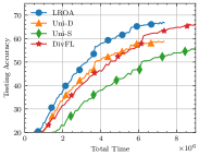
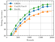
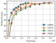
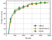
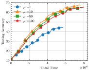
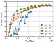
The testing accuracy w.r.t. running time and communication round for CIFAR-10 and FEMNIST are shown in Fig. 1 and Fig. 2, respectively. Here we fix $\mu=1.0$ and $\nu=10^{5}$ for CIFAR-10 and FEMNIST. Note we set the same $\mu,\nu$ for Uni-D for easy comparison. In order to provide a clearer representation of the ending points of each curve, we have included a solid circle at the termination of each curve. From the figures, we can observe LROA can achieve better testing accuracy in terms of total training latency. Specifically, LROA saves $20.8\%$ and $50.1\%$ total training time compared with Uni-D and Uni-S for CIFAR-10, and $15.3\%$ and $49.9\%$ for FEMNIST.

Note Uni-D adopts the same strategy to assign the communication power and CPU frequency as LROA, except for client sampling. Therefore, the enhancement observed from Uni-D to LROA demonstrates the effectiveness of adaptive client sampling. On the other hand, Uni-S employs fixed communication power and CPU frequency. Consequently, the improvement from Uni-S to Uni-D confirms the benefit of control in communication power and CPU frequency.

VII-B2 Comparing Different Configurations of $\lambda$ and $V$

We proceed by examining the impact of the parameter $\lambda$. The value of $\mu$ is varied across $\{1.0,10.0,50.0,100.0\}$ for CIFAR-10 dataset, and $\{0.3,0.5,5.0,10.0\}$ for FEMNIST dataset. The value of $\nu$ fixed at $10^{5}$ for both datasets. In Fig. 3, we compare the performance of LROA with baseline methods. The results illustrate that as $\lambda$ increases, the total time cost required to complete $T$ rounds also increases. Furthermore, higher values of $\lambda$ lead to improved testing accuracy. It is important to note that when $\lambda$ approaches zero, the contribution of the loss function in the objective of Problem P2 tends to diminish, which means resource allocation solely. Observing the figure, we can deduce that a smaller $\mu$ yields a highly volatile curve, particularly noticeable when $\mu=0.3$, which exhibits significant instability. This observation emphasizes the necessity of jointly considering model training and resource control.
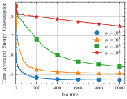
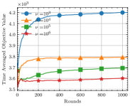
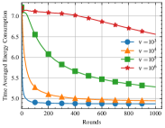
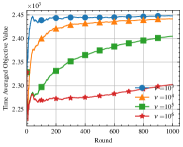
Next, we study the impact of V𝑉V. In Fig. 4, we plot the time-averaged energy consumption t=0T1(1(1qnt)K)(nt,com+nt,cmp)/Tsuperscriptsubscript𝑡0𝑇11superscript1superscriptsubscript𝑞𝑛𝑡𝐾superscriptsubscript𝑛𝑡comsuperscriptsubscript𝑛𝑡cmp𝑇\sum_{t=0}^{T-1}(1-(1-q_{n}^{t})^{K})(\mathcal{E}_{n}^{t,\text{com}}+\mathcal{E}_{n}^{t,\text{cmp}})/T and the time-averaged objective value (qnt𝒯nt+λwn2/qnt)/Tsuperscriptsubscript𝑞𝑛𝑡superscriptsubscript𝒯𝑛𝑡𝜆superscriptsubscript𝑤𝑛2superscriptsubscript𝑞𝑛𝑡𝑇(q_{n}^{t}\mathcal{T}_{n}^{t}+\lambda{w_{n}^{2}}/{q_{n}^{t}})/T. Note the curves are averaged across all devices here. We vary ν{103,104,105,106}𝜈superscript103superscript104superscript105superscript106\nu\in\{10^{3},10^{4},10^{5},10^{6}\}. As shown in Fig. 4(a), larger ν𝜈\nu results in a slower convergence rate target to energy budget, which means bad satisfaction with energy constraints. Note the energy budget is ¯n=15 Jsubscript¯𝑛times15J\bar{\mathcal{E}}_{n}=$15\text{\,}\mathrm{J}$ for CIFAR-10, ¯n=5 Jsubscript¯𝑛times5J\bar{\mathcal{E}}_{n}=$5\text{\,}\mathrm{J}$ for FEMNIST. From Fig. 4(b), we can find that large V𝑉V results in a small time-averaged objective value, which means good optimization results in terms of running time. Clearly, V𝑉V controls the trade-off between objective minimization and constraint satisfaction as stated in Section VI-A.

Refer to caption
(a) CIFAR-10
Refer to caption
(b) FEMNIST
Figure 3: Testing accuracy vs. total time of LROA under different $\lambda$ on CIFAR-10 (a) and FEMNIST (b).
Refer to caption
(a) CIFAR-10
Refer to caption
(b) CIFAR-10
Refer to caption
(c) FEMNIST
Refer to caption
(d) FEMNIST
Figure 4: Convergence of energy and objective value for CIFAR-10 (a,b) and FEMNIST (c,d). (a,c) Expected time-averaged energy consumption. (b,d) Expected time averaged objective value. $\mu=1.0$ and $\nu\in\{10^{3},10^{4},10^{5},10^{6}\}$.
Refer to caption
(a) CIFAR-10
Refer to caption
(b) FEMNIST
Figure 5: Testing accuracy vs. total time of LROA under different sampling numbers $K$ on CIFAR-10 (a) and FEMNIST (b). The marker shows the ending point of each curve. (Circle: LROA, Square: Uni-D)
Refer to caption
(a) CIFAR-10
Refer to caption
(b) FEMNIST
Figure 6: Testing accuracy vs. communication round of LROA under different sampling numbers $K$ on CIFAR-10 (a) and FEMNIST (b).

VII-B3 Impact of $K$

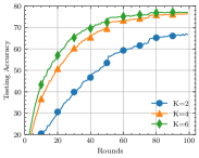
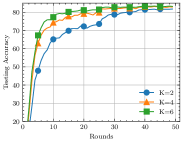
We evaluate the performance of LROA across different server sampling frequencies $K$. The range of $K$ is varied to $\{2,4,6\}$. As demonstrated in the previous experiment, the hyperparameters $\lambda$ and $V$ play a crucial role in surpassing the performance of baselines. For each $K$, we conduct a grid search to identify the optimal values within range $\mu\in\{0.1,1.0,10.0\}$ and $\nu\in\{10^{4},10^{5},10^{6}\}$. It should be noted that the corresponding values of $\lambda_{0}$ and $V_{0}$ are recalculated accordingly. We select the hyperparameter combination that hits the best time-accuracy trade-off to represent the true performance of LROA.

Specifically, since both the total running time and the final testing accuracy are critical in evaluating our algorithm, we aim to strike a balance between them. We first filter out the curves that do not meet the testing accuracy criteria. Then, we sort the remaining curves based on their total running time and select the one with the minimum value as the optimal choice. In our experiments, we define the filter-out criteria for $K\in\{2,4,6\}$ as $\{64,76,77\}$ for CIAFR-10 and $\{80,81,82\}$ for FEMNIST.

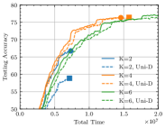
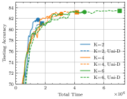
The previous experiment results have already demonstrated that the Uni-D model consistently outperforms the Uni-S and DivFL. Therefore, for the sake of simplicity, we only display the results for the Uni-D. To ensure a fair comparison, we also search for the optimal values of $\mu$ and $\nu$ for the Uni-D model within the same range, following the same principles. The results are depicted in Fig. 5 and 6.

From the figures, we can observe that our algorithm consistently outperforms the baseline algorithm across various sampling numbers $K$. This further validates the superiority of our proposed algorithm. Additionally, we notice that as $K$ increases, more communication time is required. The reason is that with more devices joining the learning, less communication bandwidth is available to a single device. Another possible reason is that, under the default setting, all devices are assumed to have the same communication and communication resources, except for different communication channels. Our problem becomes a channel selection problem. As more devices are selected, there is a higher likelihood of selecting a device with a poor channel. Furthermore, we observe that the final testing accuracy improves with increasing $K$, which aligns with our theoretical analysis presented in Theorem 1.

References

  • [1] B. McMahan, E. Moore, D. Ramage, S. Hampson, and B. A. y Arcas, “Communication-efficient learning of deep networks from decentralized data,” in Artificial intelligence and statistics.   PMLR, 2017, pp. 1273–1282.
  • [2] T. Li, A. K. Sahu, M. Zaheer, M. Sanjabi, A. Talwalkar, and V. Smith, “Federated optimization in heterogeneous networks,” Proceedings of Machine Learning and Systems, vol. 2, pp. 429–450, 2020.
  • [3] Y. G. Rui Hu, Yanmin Gong, “Federated learning with sparsification-amplified privacy and adaptive optimization.” in IJCAI, 2021.
  • [4] Z. Zhang, Y. Guo, Y. Fang, and Y. Gong, “Communication and energy efficient wireless federated learning with intrinsic privacy,” IEEE Transactions on Dependable and Secure Computing, 2023.
  • [5] S. Chen, C. Shen, L. Zhang, and Y. Tang, “Dynamic aggregation for heterogeneous quantization in federated learning,” IEEE Transactions on Wireless Communications, vol. 20, no. 10, pp. 6804–6819, 2021.
  • [6] Z. Zhang, Z. Gao, Y. Guo, and Y. Gong, “Scalable and low-latency federated learning with cooperative mobile edge networking,” IEEE Transactions on Mobile Computing, 2022.
  • [7] L. Wang, S. Xu, X. Wang, and Q. Zhu, “Addressing class imbalance in federated learning,” in 35th AAAI Conference on Artificial Intelligence (AAAI’21), 2021.
  • [8] M. Yang, X. Wang, H. Zhu, H. Wang, and H. Qian, “Federated learning with class imbalance reduction,” in 2021 29th European Signal Processing Conference (EUSIPCO).   IEEE, 2021, pp. 2174–2178.
  • [9] S. P. Karimireddy, S. Kale, M. Mohri, S. Reddi, S. Stich, and A. T. Suresh, “Scaffold: Stochastic controlled averaging for federated learning,” in International Conference on Machine Learning.   PMLR, 2020, pp. 5132–5143.
  • [10] T. Li, S. Hu, A. Beirami, and V. Smith, “Ditto: Fair and robust federated learning through personalization,” in International Conference on Machine Learning.   PMLR, 2021, pp. 6357–6368.
  • [11] Y. Guo, Y. Sun, R. Hu, and Y. Gong, “Hybrid local sgd for federated learning with heterogeneous communications,” in International Conference on Learning Representations, 2022.
  • [12] Z. Yang, M. Chen, W. Saad, C. S. Hong, and M. Shikh-Bahaei, “Energy efficient federated learning over wireless communication networks,” IEEE Transactions on Wireless Communications, vol. 20, no. 3, pp. 1935–1949, 2020.
  • [13] N. H. Tran, W. Bao, A. Zomaya, M. N. Nguyen, and C. S. Hong, “Federated learning over wireless networks: Optimization model design and analysis,” in IEEE INFOCOM 2019-IEEE conference on computer communications.   IEEE, 2019, pp. 1387–1395.
  • [14] C. T. Dinh, N. H. Tran, M. N. Nguyen, C. S. Hong, W. Bao, A. Y. Zomaya, and V. Gramoli, “Federated learning over wireless networks: Convergence analysis and resource allocation,” IEEE/ACM Transactions on Networking, vol. 29, no. 1, pp. 398–409, 2020.
  • [15] V.-D. Nguyen, S. K. Sharma, T. X. Vu, S. Chatzinotas, and B. Ottersten, “Efficient federated learning algorithm for resource allocation in wireless iot networks,” IEEE Internet of Things Journal, vol. 8, no. 5, pp. 3394–3409, 2020.
  • [16] B. Luo, X. Li, S. Wang, J. Huang, and L. Tassiulas, “Cost-effective federated learning in mobile edge networks,” IEEE Journal on Selected Areas in Communications, vol. 39, no. 12, pp. 3606–3621, 2021.
  • [17] ——, “Cost-effective federated learning design,” in IEEE INFOCOM 2021-IEEE Conference on Computer Communications.   IEEE, 2021, pp. 1–10.
  • [18] W. Chen, S. Horváth, and P. Richtárik, “Optimal client sampling for federated learning,” Transactions on Machine Learning Research, 2022. [Online]. Available: https://openreview.net/forum?id=8GvRCWKHIL
  • [19] E. Rizk, S. Vlaski, and A. H. Sayed, “Federated learning under importance sampling,” IEEE Transactions on Signal Processing, vol. 70, pp. 5381–5396, 2022.
  • [20] H. T. Nguyen, V. Sehwag, S. Hosseinalipour, C. G. Brinton, M. Chiang, and H. V. Poor, “Fast-convergent federated learning,” IEEE Journal on Selected Areas in Communications, vol. 39, no. 1, pp. 201–218, 2020.
  • [21] Y. J. Cho, J. Wang, and G. Joshi, “Client selection in federated learning: Convergence analysis and power-of-choice selection strategies,” 2021. [Online]. Available: https://openreview.net/forum?id=PYAFKBc8GL4
  • [22] B. Luo, W. Xiao, S. Wang, J. Huang, and L. Tassiulas, “Tackling system and statistical heterogeneity for federated learning with adaptive client sampling,” in IEEE INFOCOM 2022-IEEE Conference on Computer Communications.   IEEE, 2022, pp. 1739–1748.
  • [23] J. Perazzone, S. Wang, M. Ji, and K. S. Chan, “Communication-efficient device scheduling for federated learning using stochastic optimization,” in IEEE INFOCOM 2022 - IEEE Conference on Computer Communications, 2022, pp. 1449–1458.
  • [24] S. Wang, J. Perazzone, M. Ji, and K. Chan, “Federated learning with flexible control,” in IEEE Conference on Computer Communications, 2023.
  • [25] X. Deng, J. Li, C. Ma, K. Wei, L. Shi, M. Ding, W. Chen, and H. V. Poor, “Blockchain assisted federated learning over wireless channels: Dynamic resource allocation and client scheduling,” IEEE Transactions on Wireless Communications, 2022.
  • [26] X. Li, K. Huang, W. Yang, S. Wang, and Z. Zhang, “On the convergence of fedavg on non-iid data,” arXiv preprint arXiv:1907.02189, 2019.
  • [27] H. Yu, S. Yang, and S. Zhu, “Parallel restarted sgd with faster convergence and less communication: Demystifying why model averaging works for deep learning,” in Proceedings of the AAAI Conference on Artificial Intelligence, vol. 33, no. 01, 2019, pp. 5693–5700.
  • [28] S. U. Stich, “Local sgd converges fast and communicates little,” in ICLR 2019-International Conference on Learning Representations, no. CONF, 2019.
  • [29] X. Li, K. Huang, W. Yang, S. Wang, and Z. Zhang, “On the convergence of fedavg on non-iid data,” in International Conference on Learning Representations, 2020.
  • [30] R. Ward, X. Wu, and L. Bottou, “Adagrad stepsizes: Sharp convergence over nonconvex landscapes,” The Journal of Machine Learning Research, vol. 21, no. 1, pp. 9047–9076, 2020.
  • [31] L. Bottou, F. E. Curtis, and J. Nocedal, “Optimization methods for large-scale machine learning,” Siam Review, vol. 60, no. 2, pp. 223–311, 2018.
  • [32] M. J. Neely, “Stochastic network optimization with application to communication and queueing systems,” Synthesis Lectures on Communication Networks, vol. 3, no. 1, pp. 1–211, 2010.
  • [33] M. Razaviyayn, M. Hong, and Z.-Q. Luo, “A unified convergence analysis of block successive minimization methods for nonsmooth optimization,” SIAM Journal on Optimization, vol. 23, no. 2, pp. 1126–1153, 2013.
  • [34] G. Scutari, F. Facchinei, and L. Lampariello, “Parallel and distributed methods for constrained nonconvex optimization—part i: Theory,” IEEE Transactions on Signal Processing, vol. 65, no. 8, pp. 1929–1944, 2016.
  • [35] S. Boyd, S. P. Boyd, and L. Vandenberghe, Convex optimization.   Cambridge university press, 2004.
  • [36] T. T. Vu, D. T. Ngo, N. H. Tran, H. Q. Ngo, M. N. Dao, and R. H. Middleton, “Cell-free massive mimo for wireless federated learning,” IEEE Transactions on Wireless Communications, vol. 19, no. 10, pp. 6377–6392, 2020.
  • [37] S. Caldas, P. Wu, T. Li, J. Konečnỳ, H. B. McMahan, V. Smith, and A. Talwalkar, “LEAF: A benchmark for federated settings,” in Workshop on Federated Learning for Data Privacy and Confidentiality, 2019.
  • [38] A. Krizhevsky and G. Hinton, “Learning multiple layers of features from tiny images,” Master’s thesis, Department of Computer Science, University of Toronto, 2009.
  • [39] S. Caldas, S. M. K. Duddu, P. Wu, T. Li, J. Konečnỳ, H. B. McMahan, V. Smith, and A. Talwalkar, “Leaf: A benchmark for federated settings,” arXiv preprint arXiv:1812.01097, 2018.
  • [40] T.-M. H. Hsu, H. Qi, and M. Brown, “Measuring the effects of non-identical data distribution for federated visual classification,” arXiv preprint arXiv:1909.06335, 2019.
  • [41] K. He, X. Zhang, S. Ren, and J. Sun, “Deep residual learning for image recognition,” in Proceedings of the IEEE conference on computer vision and pattern recognition, 2016, pp. 770–778.
  • [42] R. Balakrishnan, T. Li, T. Zhou, N. Himayat, V. Smith, and J. Bilmes, “Diverse client selection for federated learning via submodular maximization,” in International Conference on Learning Representations, 2022.

Appendix A Proof of Equation( 4)

We take the expectation for the aggregated model $\bm{\theta}^{t+1}$ over the randomness of client sampling, we have

$\displaystyle\mathbb{E}_{\mathcal{K}^{t}}[\bm{\theta}^{t+1}]=\mathbb{E}_{\mathcal{K}^{t}}[\bm{\theta}^{t}+\sum_{n\in\mathcal{K}^{t}}\frac{w_{n}}{Kq_{n}^{t}}(\bm{\theta}_{n}^{t,E}-\bm{\theta}^{t})]$
$\displaystyle\stackrel{{\scriptstyle\textnormal{(a)}}}{{\mathstrut{=}}}\bm{\theta}^{t}+K\sum_{n=1}^{N}q_{n}^{t}\frac{w_{n}}{Kq_{n}^{t}}(\bm{\theta}_{n}^{t,E}-\bm{\theta}^{t})=\sum_{n=1}^{N}w_{n}\bm{\theta}_{n}^{t,E}=\bm{\bar{\theta}}^{t+1}.$

Here $\bm{\bar{\theta}}^{t+1}$ denotes the weighted aggregation model under full client participation. (A) is derived by examining the contribution of individual clients. As every client can be selected by the same probability $q_{n}^{t}$ and sampling $K$ times, the expectation is $K\sum_{n=1}^{N}q_{n}^{t}\frac{w_{n}}{Kq_{n}^{t}}(\bm{\theta}_{n}^{t,E}-\bm{\theta}^{t})$.

Appendix B Proof of Theorem 1

B-A Useful Lemmas

Lemma 2.

For given two vectors $\bm{a},\bm{b}\in\mathbb{R}^{d}$,

$$\|\bm{a}+\bm{b}\|^{2}\leq(1+\alpha)\|\bm{a}\|^{2}+(1+\alpha^{-1})\|\bm{b}\|^{2},\forall\alpha\geq 0.$$
Lemma 3 (Unbiased sampling and Bounded expectation).

Suppose the devices set $\mathcal{K}^{t}$ are sampled with probability $\bm{q}^{t}=[q_{1}^{t},\dots,q_{n}^{t}]$ and their local models are $\bm{\theta}_{n}^{t}$, we have

$\displaystyle\mathbb{E}_{\mathcal{K}^{t}}\sum_{n\in{\mathcal{K}^{t}}}\frac{w_{n}}{Kq_{n}}\bm{\theta}_{n}^{t}$ $\displaystyle=\sum_{n=1}^{N}w_{n}\bm{\theta}_{n}^{t}$
$\displaystyle\mathbb{E}_{\mathcal{K}^{t}}\|\sum_{n\in{\mathcal{K}^{t}}}\frac{w_{n}}{Kq_{n}}\bm{\theta}_{n}^{t}\|^{2}$ $\displaystyle\leq\sum_{n=1}^{N}\frac{w_{n}^{2}}{Kq_{n}}\|\bm{\theta}_{n}^{t}\|^{2}$
Proof:

Let $\mathcal{K}^{t}=\{n_{1},n_{2},\dots,n_{K}\}\subset[N]$. We have

$\displaystyle\mathbb{E}_{{\mathcal{K}^{t}}}\sum_{n\in{\mathcal{K}^{t}}}\frac{w_{n}}{Kq_{n}}\bm{\theta}_{n}^{t}=\mathbb{E}_{{\mathcal{K}^{t}}}\sum_{n=1}^{K}\frac{w_{n_{i}}}{Kq_{n_{i}}}\bm{\theta}_{n_{i}}^{t}=K\mathbb{E}_{{\mathcal{K}^{t}}}[\frac{w_{n_{1}}}{Kq_{n_{1}}}\bm{\theta}_{n_{1}}^{t}]$
$\displaystyle=K\sum_{n=1}^{N}\frac{w_{n}}{Kq_{n}}q_{n}\bm{\theta}_{n}^{t}=\sum_{n=1}^{N}w_{n}\bm{\theta}_{n}^{t}.$

For the expectation of square variables, we get

$\displaystyle\mathbb{E}_{\mathcal{K}^{t}}\|\sum_{n\in{\mathcal{K}^{t}}}\frac{w_{n}}{Kq_{n}}\bm{\theta}_{n}^{t}\|^{2}=\frac{1}{K^{2}}\mathbb{E}_{\mathcal{K}^{t}}\|\sum_{i=1}^{K}\frac{w_{n_{i}}}{q_{n_{i}}}\bm{\theta}_{n_{i}}^{t}\|^{2}$
$\displaystyle\stackrel{{\scriptstyle\textnormal{(b)}}}{{\mathstrut{\leq}}}\frac{1}{K}\mathbb{E}_{\mathcal{K}^{t}}\|\frac{w_{n_{1}}}{q_{n_{1}}}\bm{\theta}_{n_{1}}^{t}\|^{2}=\frac{1}{K}\sum_{n=1}^{N}\frac{w_{n}^{2}}{q_{n}^{2}}q_{n}\|\bm{\theta}_{n}^{t}\|^{2}$
$\displaystyle=\sum_{n=1}^{N}\frac{w_{n}^{2}}{Kq_{n}}\|\bm{\theta}_{n}^{t}\|^{2},$

where (B-A) follows from Cauchy-Schwarz inequality. ∎

Lemma 4 (Bounded Local Divergence).

Under Assumptions 1 and 3, if the local learning rate $\eta\leq{1}/({2\sqrt{2}E\beta})$, then the local model difference at round $t$ is bounded as follows:

$\displaystyle\sum_{n=1}^{N}\mathbb{E}[w_{n}\|\bm{\theta}^{t}-\bm{\theta}_{n}^{t,s}\|^{2}]\leq 16\eta^{2}E^{2}\gamma^{2}\|\nabla F(\bm{\theta}^{t})\|^{2}+16\eta^{2}E^{2}\kappa^{2}.$
Proof:

According to the local update rule, we have

$\displaystyle\mathbb{E}$ $\displaystyle\|\bm{\theta}^{t}-\bm{\theta}_{n}^{t,s}\|^{2}=\mathbb{E}\|\bm{\theta}_{n}^{t,s-1}-\bm{\theta}^{t}-\eta\nabla F_{n}(\bm{\theta}_{n}^{t,s-1})$
$\displaystyle+\eta\nabla F_{n}(\bm{\theta}^{t})-\eta\nabla F_{n}(\bm{\theta}^{t})\|^{2}$
$\displaystyle\stackrel{{\scriptstyle\textnormal{(c)}}}{{\mathstrut{\leq}}}$ $\displaystyle(1+\frac{1}{2E-1})\mathbb{E}\|\bm{\theta}_{n}^{t,s-1}-\bm{\theta}^{t}\|^{2}$
$\displaystyle+2\eta^{2}E\mathbb{E}\|\nabla F_{n}(\bm{\theta}_{n}^{t,s-1})+\nabla F_{n}(\bm{\theta}^{t})-\nabla F_{n}(\bm{\theta}^{t})\|^{2}$
$\displaystyle\stackrel{{\scriptstyle\textnormal{(d)}}}{{\mathstrut{\leq}}}$ $\displaystyle(1+\frac{1}{2E-1})\mathbb{E}\|\bm{\theta}_{n}^{t,s-1}-\bm{\theta}^{t}\|^{2}$
$\displaystyle+4\eta^{2}E\mathbb{E}\|\nabla F_{n}(\bm{\theta}_{n}^{t,s-1})-\nabla F_{n}(\bm{\theta}^{t})\|^{2}+4\eta^{2}E\mathbb{E}\|\nabla F_{n}(\bm{\theta}^{t})\|^{2}$
$\displaystyle\stackrel{{\scriptstyle\textnormal{(e)}}}{{\mathstrut{\leq}}}$ $\displaystyle(1+\frac{1}{2E-1})\mathbb{E}\|\bm{\theta}_{n}^{t,s-1}-\bm{\theta}^{t}\|^{2}$
$\displaystyle+4\eta^{2}\beta^{2}E\mathbb{E}\|\bm{\theta}_{n}^{t,s-1}-\bm{\theta}^{t}\|^{2}+4\eta^{2}E\mathbb{E}\|\nabla F_{n}(\bm{\theta}^{t})\|^{2}$

where (B-A) follows from Lemma 2 with $\alpha={1}/({2E-1})$, (B-A) follows from Cauchy-Schwarz inequality, and (B-A) follows from Assumption 1. Next, we get

$\displaystyle\sum_{n=1}^{N}\mathbb{E}w_{n}\|\bm{\theta}^{t}-\bm{\theta}_{n}^{t,s}\|^{2}\stackrel{{\scriptstyle\textnormal{(f)}}}{{\mathstrut{\leq}}}4\eta^{2}E\gamma^{2}\mathbb{E}\|\nabla F(\bm{\theta}^{t})\|^{2}+4\eta^{2}E\kappa^{2}$
$\displaystyle+(1+\frac{1}{2E-1}+4\eta^{2}\beta^{2}E)\sum_{n=1}^{N}\mathbb{E}w_{n}\|\bm{\theta}_{n}^{t,s-1}-\bm{\theta}^{t}\|^{2}$

where (B-A) holds due to Assumption 3. When $\eta\leq{1}/({2\sqrt{2}E\beta})$, then $4\eta^{2}\beta^{2}E\leq{1}/({2E})$, we have

$\displaystyle\sum_{n=1}^{N}\mathbb{E}w_{n}\|\bm{\theta}^{t}-\bm{\theta}_{n}^{t,s}\|^{2}\leq$ $\displaystyle(1+\frac{1}{E-1})\sum_{n=1}^{N}\mathbb{E}w_{n}\|\bm{\theta}_{n}^{t,s-1}-\bm{\theta}^{t}\|^{2}$
$\displaystyle+4\eta^{2}E\gamma^{2}\mathbb{E}\|\nabla F(\bm{\theta}^{t})\|^{2}+4\eta^{2}E\kappa^{2}.$

Unrolling the recursion, we get

$\displaystyle\sum_{n=1}^{N}\mathbb{E}w_{n}\|\bm{\theta}^{t}-\bm{\theta}_{n}^{t,s}\|^{2}$
$\displaystyle\leq\sum_{h=1}^{s-1}(1+\frac{1}{E-1})^{h}\left[4\eta^{2}E\gamma^{2}\mathbb{E}\|\nabla F(\bm{\theta}^{t})\|^{2}+4\eta^{2}E\kappa^{2}\right]$
$\displaystyle\leq(E-1)\left[(1+\frac{1}{E-1})^{E}-1\right]\cdot[4\eta^{2}E\gamma^{2}\mathbb{E}\|\nabla F(\bm{\theta}^{t})\|^{2}$
$\displaystyle\quad+4\eta^{2}E\kappa^{2}]$
$\displaystyle\stackrel{{\scriptstyle\textnormal{(g)}}}{{\mathstrut{\leq}}}16\eta^{2}E^{2}\gamma^{2}\|\nabla F(\bm{\theta}^{t})\|^{2}+16\eta^{2}E^{2}\kappa^{2},$

where (B-A) follows from $(1+\frac{1}{E-1})^{E}\leq 5$ when $E\geq 1$. ∎

B-B Proof of Theorem 1

Proof:

According to Assumption 1, we have

$\displaystyle\mathbb{E}[F(\bm{\theta}^{t+1}-F(\bm{\theta}^{t})]$
$\displaystyle\leq\mathbb{E}\langle\nabla F(\bm{\theta}^{t}),\bm{\theta}^{t+1}-\bm{\theta}^{t}\rangle+\frac{\beta}{2}\mathbb{E}\|\bm{\theta}^{t+1}-\bm{\theta}^{t}\|^{2}$
$\displaystyle=\mathbb{E}\langle\nabla F(\bm{\theta}^{t}),\mathbb{E}_{\mathcal{K}^{t}}\sum_{n\in\mathcal{K}^{t}}\frac{w_{n}}{Kq_{n}}(\bm{\theta}_{n}^{t+1}-\bm{\theta}^{t})\rangle$
$\displaystyle\quad+\frac{\beta}{2}\mathbb{E}\|\sum_{n\in\mathcal{K}^{t}}\frac{w_{n}}{Kq_{n}}(\bm{\theta}_{n}^{t+1}-\bm{\theta}^{t})\|^{2}$
$\displaystyle\stackrel{{\scriptstyle\textnormal{(h)}}}{{\mathstrut{=}}}\underbrace{-\mathbb{E}\langle\nabla F(\bm{\theta}^{t}),\sum_{n=1}^{N}w_{n}(\eta\sum_{s=0}^{E-1}\nabla F_{n}(\bm{\theta}_{n}^{t,s}))\rangle}_{T_{1}}$
$\displaystyle\quad+\underbrace{\frac{\beta}{2}\mathbb{E}\|\sum_{n\in\mathcal{K}^{t}}\frac{w_{n}}{Kq_{n}}\eta\sum_{s=0}^{E-1}\nabla F_{n}(\bm{\theta}_{n}^{t,s})\|^{2}}_{T_{2}},$ (31)

where (B-B) holds due to Lemma 3. For $T_{1}$, we have

$\displaystyle T_{1}\stackrel{{\scriptstyle\textnormal{(i)}}}{{\mathstrut{=}}}$ $\displaystyle-\frac{\eta E}{2}\|\nabla F(\bm{\theta}^{t})\|^{2}-\frac{\eta E}{2}\|\frac{1}{E}\sum_{n=1}^{N}\sum_{s=0}^{E-1}w_{n}\nabla F_{n}(\bm{\theta}_{n}^{t,s})\|^{2}$
$\displaystyle+\frac{\eta E}{2}\|\frac{1}{E}\sum_{n=1}^{N}\sum_{s=0}^{E-1}w_{n}(\nabla F_{n}(\bm{\theta}^{t})-\nabla F_{n}(\bm{\theta}_{n}^{t,s}))\|^{2}$
$\displaystyle\stackrel{{\scriptstyle\textnormal{(j)}}}{{\mathstrut{\leq}}}$ $\displaystyle-\frac{\eta E}{2}\|\nabla F(\bm{\theta}^{t})\|^{2}$
$\displaystyle+\frac{\eta}{2}\sum_{n=1}^{N}\sum_{s=0}^{E-1}w_{n}\|\nabla F_{n}(\bm{\theta}^{t})-\nabla F_{n}(\bm{\theta}_{n}^{t,s})\|^{2}$
$\displaystyle\stackrel{{\scriptstyle\textnormal{(k)}}}{{\mathstrut{\leq}}}$ $\displaystyle-\frac{\eta E}{2}\|\nabla F(\bm{\theta}^{t})\|^{2}+\frac{\eta\beta^{2}}{2}\sum_{n=1}^{N}\sum_{s=0}^{E-1}w_{n}\|\bm{\theta}^{t}-\bm{\theta}_{n}^{t,s}\|^{2},$ (32)

where (B-B) follows from $2\langle\bm{a},\bm{b}\rangle=\|\bm{a}\|^{2}+\|\bm{b}\|^{2}-\|\bm{a}-\bm{b}\|^{2}$, (B-B) holds due to Jensen’s inequality, and (32) comes from Assumption 1. For $T_{2}$, using Lemma 3, we obtain:

$\displaystyle T_{2}=\frac{\beta}{2}\sum_{n=1}^{N}\frac{w_{n}^{2}\eta^{2}}{Kq_{n}}\|\sum_{s=0}^{E-1}\nabla F_{n}(\bm{\theta}_{n}^{t,s})\|^{2}\leq\frac{\beta\eta^{2}E^{2}G^{2}}{2K}\sum_{n=1}^{N}\frac{w_{n}^{2}}{q_{n}}.$ (33)

Combining (31), (32) and (33), we get:

$\displaystyle\mathbb{E}$ $\displaystyle[F(\bm{\theta}^{t+1}-F(\bm{\theta}^{t})]\leq-\frac{\eta E}{2}\|\nabla F(\bm{\theta}^{t})\|^{2}$
$\displaystyle+\frac{\eta\beta^{2}}{2}\sum_{n=1}^{N}\sum_{s=0}^{E-1}w_{n}\|\bm{\theta}^{t}-\bm{\theta}_{n}^{t,s}\|^{2}+\frac{\beta\eta^{2}E^{2}G^{2}}{2K}\sum_{n=1}^{N}\frac{w_{n}^{2}}{q_{n}}$
$\displaystyle\leq$ $\displaystyle-\frac{\eta E}{2}\|\nabla F(\bm{\theta}^{t})\|^{2}+\frac{\beta\eta^{2}E^{2}G^{2}}{2K}\sum_{n=1}^{N}\frac{w_{n}^{2}}{q_{n}}$
$\displaystyle+\frac{\eta\beta^{2}E}{2}(16\eta^{2}E^{2}\gamma^{2}\|\nabla F(\bm{\theta}^{t})\|^{2}+16\eta^{2}E^{2}\kappa^{2})$
$\displaystyle=$ $\displaystyle(-\frac{\eta E}{2}+8\eta^{3}\beta^{2}\gamma^{2}E^{3})\|\nabla F(\bm{\theta}^{t})\|^{2}+8\eta^{3}\beta^{2}E^{3}\kappa^{2}$
$\displaystyle+\frac{\beta\eta^{2}E^{2}G^{2}}{2K}\sum_{n=1}^{N}\frac{w_{n}^{2}}{q_{n}}.$

If taking $\eta\leq{1}/({32E^{2}\beta^{2}\gamma^{2}})$, then we have:

$\displaystyle\mathbb{E}[F(\bm{\theta}^{t+1}-F(\bm{\theta}^{t})]\leq$ $\displaystyle-\frac{\eta E}{4}\|\nabla F(\bm{\theta}^{t})\|^{2}+8\eta^{3}\beta^{2}E^{3}\kappa^{2}$
$\displaystyle+\frac{\beta\eta^{2}E^{2}G^{2}}{2K}\sum_{n=1}^{N}\frac{w_{n}^{2}}{q_{n}}.$

Summing the above inequality from $t=0,\dots,T-1$ and rearranging it, we obtain:

$\displaystyle\sum_{t=0}^{T-1}\|\nabla F(\bm{\theta}^{t})\|^{2}\leq$ $\displaystyle\frac{4(F(\bm{\theta}^{0})-F^{*})}{\eta E}+8T\eta^{2}\beta^{2}E^{2}\kappa^{2}$ (34)
$\displaystyle+\frac{2\beta\eta EG^{2}}{K}\sum_{t=0}^{T-1}\sum_{n=1}^{N}\frac{w_{n}^{2}}{q_{n}^{t}}.$

Dividing both sides by $T$, we get the final result. ∎

Appendix C Proof of Lemma 1

Proof:

By squaring the virtual queue $Q_{n}^{t+1}=\max\{Q_{n}^{t}+a_{n}^{t},0\}$, we have:

$\displaystyle(\max\{Q_{n}^{t}+a_{n}^{t},0\})^{2}\leq(Q_{n}^{t})^{2}+(a_{n}^{t})^{2}+2Q_{n}^{t}a_{n}^{t}.$

Then, we obtain:

$\displaystyle\frac{(Q_{n}^{t+1})^{2}-(Q_{n}^{t})^{2}}{2}\leq\frac{(a_{n}^{t})^{2}}{2}+Q_{n}^{t}a_{n}^{t}.$ (35)

For $a_{n}^{t}$, we have:

$\displaystyle a_{n}^{t}$ $\displaystyle=(1-(1-q_{n}^{t})^{K})(\mathcal{E}_{n}^{t,\text{cmp}}+\mathcal{E}_{n}^{t,\text{com}})-\bar{\mathcal{E}}_{n}$
$\displaystyle=(1-(1-q_{n}^{t})^{K})(\frac{E\alpha_{n}c_{n}D_{n}(f_{n}^{t})^{2}}{2}+p_{n}^{t}\mathcal{T}_{n,u}^{t,\text{com}})-\bar{\mathcal{E}}_{n}.$

According to the formula $(x-y)^{2}\leq x^{2}+y^{2}(x,y\geq 0)$ and $(1-(1-q_{n}^{t})^{K})\leq 1$, we have:

$\displaystyle(a_{n}^{t})^{2}$ $\displaystyle\leq\left[\frac{E\alpha_{n}c_{n}D_{n}(f_{n}^{t})^{2}}{2}+p_{n}^{t}\mathcal{T}_{n,u}^{t,\text{com}}\right]^{2}+(\bar{\mathcal{E}}_{n})^{2}$
$\displaystyle\leq\left[\bar{\mathcal{T}}_{n}^{t,\text{com}}p_{n}^{\max}+\frac{E\alpha_{n}c_{n}D_{n}(f_{n}^{\max})^{2}}{2}\right]^{2}+(\bar{\mathcal{E}}_{n})^{2}$

where $\bar{\mathcal{T}}_{n}^{t,\text{com}}$ is the upper bound of $\mathcal{T}_{n,u}^{t,\text{com}}$. Summing over all devices, taking the expectation w.r.t $\bm{Q}^{t}$ on both sides, and adding penalty term $V\mathbb{E}\left\{\sum_{n=1}^{N}\left(q_{n}^{t}\mathcal{T}_{n}^{t}+\lambda\cdot\frac{w_{n}^{2}}{q_{n}^{t}}\right)|\bm{Q}^{t}\right\}$ to both sides of the inequality (35), we get the final result. ∎

Appendix D Proof of Theorem 2

Proof:

Problem 3.1.1 can be rewritten as

$\displaystyle\min_{\{f_{n}^{t}\}}\quad\sum_{n=1}^{N}\frac{\Omega_{1,n}}{f_{n}^{t}}+\sum_{n=1}^{N}\Omega_{2,n}(f_{n}^{t})^{2}$
$\displaystyle\text{s.t.}\qquad f_{n}^{\min}\leq f_{n}^{t}\leq f_{n}^{\max},\quad\forall n\in[N],$

where $\Omega_{1,n}$ and $\Omega_{2,n}$ are positive constants denoted by $\Omega_{1,n}=VEq_{n}^{t}c_{n}D_{n},\Omega_{2,n}=\frac{1}{2}Q_{n}^{t}(1-(1-q_{n}^{t})^{K})E\alpha_{n}c_{n}D_{n}$. Taking the first-order derivation of the objective function, we obtain

$\displaystyle-\frac{\Omega_{1,n}}{(f_{n}^{t})^{2}}+2\Omega_{2,n}f_{n}^{t}=0,\quad f_{n}^{t}=\left(\frac{\Omega_{1,n}}{2\Omega_{2,n}}\right)^{\frac{1}{3}}$ (36)

Then, for the second-order derivation, we have

$\displaystyle 2\frac{\Omega_{1,n}}{(f_{n}^{t})^{3}}+2\Omega_{2,n}>0.$

So the root in (36) is the global minimum. In final, we obtain

$\displaystyle(f_{n}^{t})^{*}=\min\{\max\{\left(\frac{Vq_{n}^{t}}{Q_{n}^{t}\big{[}(1-(1-q_{n}^{t})^{K}]\alpha_{n}}\right)^{\frac{1}{3}},f_{n}^{\min}\},f_{n}^{\max}\}.$

Appendix E Proof of Theorem 3

Proof:

Problem P3.1.2 can be rewritten as

$\displaystyle\min_{\{x_{n}^{t}\}}\quad$ $\displaystyle\sum_{n=1}^{N}\Omega_{3,n}\frac{x_{n}^{t}+A_{1,n}}{\log_{2}{(1+x_{n}^{t}})}$ (37)
s.t. $\displaystyle\frac{h_{n}^{t}p_{n}^{\min}}{N_{0}}\leq x_{n}^{t}\leq\frac{h_{n}^{t}p_{n}^{\max}}{N_{0}},\quad\forall n\in[N],$

where $x_{n}^{t}=\frac{h_{n}^{t}p_{n}^{t}}{N_{0}}$, $\Omega_{3,n}=\frac{MKN_{0}}{Bh_{n}^{t}}Q_{n}^{t}(1-(1-q_{n}^{t})^{K})$ and $A_{1,n}=\frac{Vq_{n}^{t}h_{n}^{t}}{Q_{n}^{t}(1-(1-q_{n}^{t})^{K})N_{0}}$ are always positive. Problem (37) can be solved by individually optimizing $x_{n}^{t}$. So taking the second-order derivation of the objective (37), we obtain

$\displaystyle\Omega_{3,n}\frac{(A_{1,n}-x_{n}^{t}-2)\ln(1+x_{n}^{t})+2(A_{1,n}+x_{n}^{t})}{(1+x_{n}^{t})^{2}\ln^{2}{(2)}\log_{2}^{3}{(1+x_{n}^{t})}}$ (38)

From the inequality $\ln(1+x)\geq\frac{x}{1+x}$, ($x>=0$) we have:

$\displaystyle(A_{1,n}-x_{n}^{t}-2)\ln(1+x_{n}^{t})+2(A_{1,n}+x_{n}^{t})$
$\displaystyle\geq\frac{(A_{1,n}-x_{n}^{t}-2)x_{n}^{t}+2(A_{1,n}+x_{n}^{t})(1+x_{n}^{t})}{1+x_{n}^{t}}$ (39)

Simplify the numerator of (39). We obtain

$\displaystyle(x_{n}^{t})^{2}+3A_{1,n}x_{n}^{t}+2A_{1,n}\geq 0,$ (40)

where the inequality holds because $x_{n}^{t},A_{1,n}$ are positive. Thus, Problem (37) is convex. To solve the problem, we take the first order derivation of the objective function (37), we have

$\displaystyle\Omega_{3,n}\frac{\log_{2}(1+x_{n}^{t})-\frac{(x_{n}^{t}+A_{1,n})}{\ln{2}(1+x_{n}^{t})}}{\log_{2}^{2}{(1+x_{n}^{t})^{2}}}=0$ (41)
$\displaystyle\ln{(1+\frac{h_{n}^{t}p_{n}^{t}}{N_{0}})}=\frac{(\frac{h_{n}^{t}p_{n}^{t}}{N_{0}}+A_{1,n})}{(1+\frac{h_{n}^{t}p_{n}^{t}}{N_{0}})}$

By solving (41) and definition of $x_{n}^{t}$, we get

$\displaystyle\ln{(1+\frac{h_{n}^{t}p_{n}^{t}}{N_{0}})}=\frac{h_{n}^{t}p_{n}^{t}+A_{1,n}N_{0}}{h_{n}^{t}p_{n}^{t}+N_{0}}$ (42)

So the root in (42) is global minimum in the first quadrant. In final, we obtain

$\displaystyle(p_{n}^{t})^{*}=\min\{\max\{(p_{n}^{t})^{\prime},p_{n}^{\min}\},p_{n}^{\max}\},$

where $(p_{n}^{t})^{\prime}$ is the root of (42). ∎