Uncertainty quantification on the prediction of
creep remaining useful life

Abstract

Accurate prediction of remaining useful life (RUL) under creep conditions is crucial for the design and maintenance of industrial equipment operating at high temperatures. Traditional deterministic methods often overlook significant variability in experimental data, leading to unreliable predictions. This study introduces a probabilistic framework to address uncertainties in predicting creep rupture time. We utilize robust regression methods to minimize the influence of outliers and enhance model estimates. Sobol indices-based global sensitivity analysis identifies the most influential parameters, followed by Monte Carlo simulations to determine the probability distribution of the material’s RUL. Model selection techniques, including the Akaike and Bayesian information criteria, ensure the optimal predictive model. This probabilistic approach allows for the delineation of safe operational limits with quantifiable confidence levels, thereby improving the reliability and safety of high-temperature applications. The framework’s versatility also allows integration with various mathematical models, offering a comprehensive understanding of creep behavior.

1 Introduction

The accurate prediction of creep remaining useful life (RUL) is critical for ensuring the reliability and safety of components operating under high temperatures in various industrial applications, such as power plants and aerospace systems [1, 2]. Traditional deterministic approaches to predicting creep rupture strength and deformation, such as time-temperature-parameter (TTP) methods, have been widely adopted and are recommended by design codes, including the ASME Boiler and Pressure Vessel Code [3, 4]. However, these methods often fail to account for significant uncertainties arising from experimental data variability and model inaccuracies, which can impact the reliability of the predictions.

Recent advancements in the field have highlighted the necessity of probabilistic methods for a more robust assessment of creep RUL. For instance, Gao et al. [5] and Wang et al. [6] have introduced surrogate modeling approaches for creep-fatigue reliability assessment, incorporating multi-source uncertainty to enhance prediction accuracy. These works underscore the importance of addressing both aleatory and epistemic uncertainties in predictive models. The presence of significant dispersion in creep data and the complexity of underlying failure mechanisms, as discussed by Roya et al. [7], further emphasizes the need for a probabilistic approach.

Traditional deterministic models often overlook the substantial variability in material properties and operational conditions, leading to potential inaccuracies in long-term predictions. Phan et al. [8] highlighted the limitations of deterministic models in capturing the stochastic nature of microscale creep deformation and rupture mechanisms. Similarly, Harlow and Delph [9] demonstrated the necessity of considering stochastic variations in constitutive modeling for more reliable creep life predictions.

The shift from deterministic to probabilistic methodologies is driven by the need for a formal consideration of uncertainties, enabling more accurate reliability and risk assessments. This transition is critical in the context of life extension for high-temperature components, where reducing conservatism without compromising safety is essential. Probabilistic methods allow for the quantification of uncertainties and the calculation of failure probabilities, providing a more comprehensive understanding of material behavior under high-temperature conditions. This approach aligns with recent studies such as those by Beck and Fadel Miguel [10], Gomes and Beck [11], and Gomes et al. [12], which emphasize the importance of reliability-based design optimization and model error considerations in structural reliability.

Previous research has explored various probabilistic methods for creep RUL prediction. Notable contributions include the probabilistic Larson-Miller creep model by Lou et al. [13] and the service condition-creep rupture property interference (SCRI) model by Zhao et al. [14]. Despite these advances, there remains a gap in the systematic treatment of outliers, global sensitivity analysis, and comprehensive uncertainty quantification in creep life predictions.

Our research aims to address these gaps by proposing a probabilistic uncertainty quantification framework for predicting high-temperature creep in metallic components. This framework employs robust regression methods to mitigate the influence of outliers and uses Sobol indices for global sensitivity analysis to identify the most influential parameters. Monte Carlo simulations are then used to establish the probability distribution of the material’s remaining useful life. The framework is versatile and can be integrated into various mathematical models, including continuum damage mechanics-based models [9, 15].

By adopting a probabilistic approach, our methodology provides a rigorous and comprehensive assessment of creep RUL, offering significant improvements over traditional deterministic methods. This approach aligns with recent studies such as those by Beck et al. [16] and Wang et al. [2], which emphasize the importance of reliability-based design optimization and data-driven reliability assessments, respectively. In this sense, this research advocates for a paradigm shift towards probabilistic methodologies in creep RUL prediction, emphasizing the identification and quantification of uncertainties to enhance the reliability and safety of high-temperature components.

The rest of this paper is organized as follows. Section 2 outlines the parametric models for creep prediction, including the Larson-Miller, Orr-Sherby-Dorn, and Manson-Succop models. Section 3 describes the proposed uncertainty quantification framework, detailing the statistical inference, sensitivity analysis, uncertainty modeling, uncertainty propagation, and model selection processes. Section 4 presents the results and discussion, including the polynomial representation of creep model parameters, key parameters, probabilistic modeling, statistical examination of material rupture time, and the identification of the optimal creep model. Finally, Section 5 concludes the paper with a summary of key findings and their implications for the field, along with suggestions for future research.

2 Parametric models for creep prediction

In this section, we outline the mathematical foundations and key assumptions of three widely-used parametric models for creep prediction: the Larson-Miller (LM), Orr-Sherby-Dorn (OSD), and Manson-Succop (MS) models. This overview, which presents a summary of these models rather than a comprehensive discussion, is intended for clarity and completeness.

2.1 The Larson-Miller Model

The Larson-Miller (LM) model [13, 17, 18, 19] is a common parametric method used to predict the rupture time of metals under creep. Deriving from the Arrhenius relation at a constant stress, the LM model considers a variable temperature $T$ and creep activation energy $Q_{c}$, resulting in the following mathematical relation

$$P_{LM}(\sigma)=T\,\left(C_{LM}+\log{t_{r}}\right)\,,$$ (1)

where $C_{LM}$ and $P_{LM}$ are the Larson-Miller constant and parameter, respectively. The $P_{LM}$ parameter allows for the superposition of rupture curves into a single master curve, a graphical representation of the logarithm of rupture time ($\log{t_{r}}$) plotted against $1/T$ at a constant stress $\sigma$ [3, 20].

While the LM model offers an effective means of predicting creep behavior, it suffers from limitations in terms of physical realism, particularly due to variations in the $C_{LM}$ constant across different alloys and processing conditions [21]. To improve reliability and account for these uncertainties, it is suggested to apply this model within a probabilistic framework as argued by Mohammad Lou et al. [13].

2.2 The Orr-Sherby-Dorn Model

The Orr-Sherby-Dorn (OSD) model [13, 19, 22] presents a unique approach where the constant in the LM equation becomes a function of stress, and the LM parameter becomes a constant. This rearrangement of the LM relation leads to the OSD equation

$$P_{OSD}(\sigma)=\log{t_{r}}-\frac{C_{OSD}}{T}\,,$$ (2)

where $P_{OSD}$ and $C_{OSD}$ are the Orr-Sherby-Dorn parameter and constant, respectively. A key assumption of the OSD model is that the creep activation energy, $Q_{c}$, remains constant over the creep curve, an assumption with limited empirical support [3, 22, 23]. The OSD model’s limitations become evident when structural instabilities and multiple rate processes are involved [3, 24, 25]. As with the LM model, these limitations suggest the need for a probabilistic approach that can accommodate uncertainties and provide more reliable predictions.

2.3 The Manson-Succop Model

The Manson-Succop (MS) model [26], based on an analysis of the iso-stress lines in a log-time versus temperature plot, defines its parameter $P_{MS}$ through the parallelism of these lines. The MS equation is given by

$$P_{MS}(\sigma)=\log(t_{r})+C_{MS}\,T\,,$$ (3)

where $P_{MS}$ and $C_{MS}$ are the Manson-Succop parameter and constant, respectively. While the MS model, similar to the LM and OSD models, provides a useful tool for predicting creep life, its deterministic nature often leads to overestimations and errors, particularly for long-term creep life predictions [3, 27]. Hence, a probabilistic approach is suggested for more accurate and safer creep life predictions.

2.4 Limitations of parametric models

The effectiveness of parametric models for creep life prediction, including the LM, OSD, and MS models, is well-documented and acknowledged [28]. Their wide application stems from their ability to reduce the costs and timelines associated with collecting long-term creep data. By extrapolating short-term creep data using a time-temperature parameter, these deterministic models form a procedure that allows for the generation of a single “master curve”. This curve, where stress is plotted against an empirical parameter that merges time and temperature, is constructed using available short-term creep data, and from this, predictions for longer durations can be extrapolated [28]. Although more mathematically simple than their continuum damage mechanics-based counterparts, these parametric methods have a great advantage, at least in theory, of requiring only a relatively small amount of data to establish the required master curve [28].

Despite their recognized utility and proved validity for long-term creep predictions, these models are not without limitations. There are several areas where these parametric models may not fully capture the complexities and uncertainties inherent in real-world scenarios, making their outputs less reliable under certain circumstances, as acknowledged by Refs. [28, 29].

The first major limitation lies in the deterministic nature of these models. They inherently assume constant material properties and unvarying loading conditions. In reality, however, both operational environments and material properties fluctuate significantly due to numerous factors. For example, manufacturing processes can introduce variations in the properties of a material. Additionally, the material inhomogeneities present in real-world scenarios can contribute to variances that these models are unable to account for. Operational uncertainties, such as temperature fluctuations or irregular loading conditions, can also significantly impact the creep behavior of materials, introducing additional sources of discrepancies between model predictions and actual outcomes.

Secondly, these models have been observed to struggle when tasked with the prediction of long-term creep life. These models are based on extrapolation of short-term creep test data obtained for larger stress levels. While useful for reducing testing time, they do not take into account that microstructural damage mechanisms induced by larger stress levels may be quite different from those verified in an actual component subjected to much lower stress levels. Hence, larger discrepancies are commonly verified when extrapolating creep life using these deterministic models, as both model-parameter uncertainties and model uncertainties induced by different microstructural damages evolving at unknown time rates are not taken into account. This dispersion means that different predictions frequently arise, even when using experimental data acquired under apparently identical macroscopic conditions. The introduction of these uncertainties in long-term forecasts can cause the models to become less accurate. The inaccuracy is often compounded in high-stress, high-temperature applications, where the creep behavior becomes notably nonlinear.

Moreover, it is worth noting that these parametric models often ignore changes in creep fracture mechanisms across different temperature ranges and fracture durations. This can lead to inaccuracies and overestimations in the projected long-term creep life. This is particularly evident in the MS model which assumes fixed values of constants over a wide range of temperatures and fracture durations.

Lastly, these models tend to oversimplify the processes they are trying to predict. Complex interactions between multiple factors affecting the creep strength of alloys, particularly at high temperatures, are often not adequately accounted for. This simplification becomes especially problematic in scenarios involving structural instabilities or where multiple rate processes are at play, such as in complex alloys.

Considering these limitations, it is necessary to adopt a probabilistic approach in order to account for the inherent uncertainties in creep life prediction. The probabilistic approach not only provides a risk-based perspective, but also optimizes design, maintenance, and operation strategies. Adopting such an approach is crucial during the initial design phase of high-temperature equipment to ensure a specific service life as determined by code. This strengthens the argument for the application of parametric models from a probabilistic perspective, leading to a more reliable and accurate prediction of creep life.

3 Uncertainty quantification framework

The uncertainty quantification (UQ) framework proposed here, inspired by the works [30], [31], and [32], encompasses a five-step process. This process, schematically illustrated in Figure 1, includes stages of statistical inference, sensitivity analysis, uncertainty modeling, uncertainty propagation, and model selection. Each of these steps is explored in greater detail below.

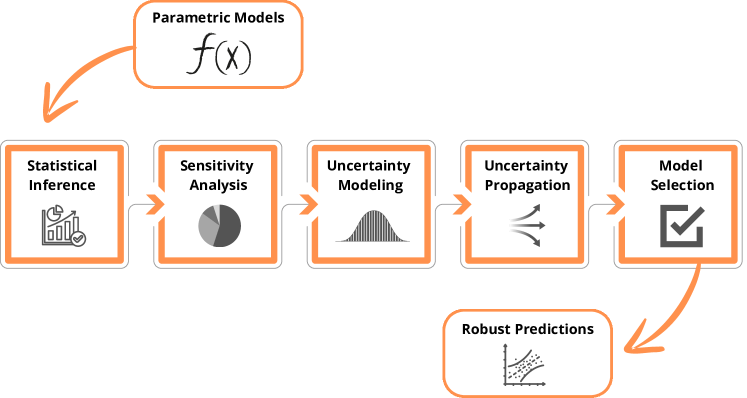
Figure 1: Schematic illustration of the probabilistic uncertainty quantification framework for creep remaining useful life prediction.

3.1 Statistical inference

The first phase in our uncertainty quantification framework involves defining the mathematical relationship between empirical parameters of deterministic creep models ($P_{LM}$, $P_{OSD}$, $P_{MS}$) and the mechanical stress, $\sigma$. The initial process involves data pre-processing to minimize the influence of potential outliers that could potentially distort the analysis. To this end, we apply the winsorization method, which has proven to be effective in controlling extreme values [33]. This technique operates by assigning all outliers to a specific percentile of the data. For instance, a 95% winsorization would set all data points below the 5th percentile to the value at the 5th percentile, and all data above the 95th percentile to the value at the 95th percentile.

After the data has been winsorized, we proceed with identifying the relationship between the creep model parameter $P_{\square}$ and the stress $\sigma$, i.e.,

$$P_{\square}=a_{0}+a_{1}\,\sigma+\cdots+a_{n-1}\,\sigma^{n-1}\,.$$ (4)

We approach this problem from a data-driven perspective, employing a specialized form of sparse regression, the sequential threshold least-square (STLS), along with cross-validation [34, 35]. The use of STLS allows for the identification of polynomial relationships between variables, free from assumptions regarding the polynomial degree. In mathematical terms, given a design matrix $[\bm{A}]\in\mathbb{R}^{m\times n}$, the observations $\bm{y}\in\mathbb{R}^{m}$, and the unknown vector $\bm{x}\in\mathbb{R}^{n}$,

$$[\bm{A}]=\begin{bmatrix}1&\sigma_{1}&\sigma_{1}^{2}&\cdots&\sigma_{1}^{n-1}\\ 1&\sigma_{2}&\sigma_{2}^{2}&\cdots&\sigma_{2}^{n-1}\\ \vdots&\vdots&\vdots&\ddots&\vdots\\ 1&\sigma_{m}&\sigma_{m}^{2}&\cdots&\sigma_{m}^{n-1}\end{bmatrix}\,,\leavevmode\nobreak\ \leavevmode\nobreak\ \bm{y}=\begin{bmatrix}P_{\square\leavevmode\nobreak\ 1}\\ P_{\square\leavevmode\nobreak\ 2}\\ \vdots\\ P_{\square\leavevmode\nobreak\ m}\end{bmatrix}\,,\leavevmode\nobreak\ \leavevmode\nobreak\ \bm{x}=\begin{bmatrix}a_{0}\\ \vdots\\ a_{n-1}\end{bmatrix}\,,$$ (5)

the STLS solves the optimization problem

$$\bm{x}^{\ast}=\arg\min_{\bm{x}\leavevmode\nobreak\ \in\leavevmode\nobreak\ \mathbb{R}^{m}}\leavevmode\nobreak\ ||\,\bm{y}-[\bm{A}]\,\bm{x}\,||_{2}^{2}+\lambda\,||\,\bm{x}\,||_{0}\,,$$ (6)

where $||.||_{2}$ denotes the $l_{2}$-norm, $||.||_{0}$ is the “$l_{0}$-norm” denoting the number of nonzero entries in a vector, and $\lambda$ is a sparsity-inducing regularization parameter. A parsimonious polynomial model emerges as a result of enforcing sparsity on the regression coefficients, eliminating redundant powers, and determining the optimal fit function based on a rational criterion.

Cross-validation is utilized to evaluate each polynomial’s predictive ability and to select the optimal model using the root mean squared error (RMSE) criterion. The cross-validation process splits the experimental data into complementary subsets, performs the analysis on one subset (the training set), and validates the analysis on the other subset (the validation or testing set). This procedure is formally described as follows: given a dataset of size $m$, it is divided into $k$ equally sized folds. For each fold $i=1,...,k$, a model is trained on all data excluding fold $i$ and is then tested on fold $i$, yielding a prediction error $e_{i}$. The RMSE is then computed as

$$RMSE=\sqrt{\frac{1}{k}\sum_{i=1}^{k}e_{i}^{2}}.$$ (7)

The data is then shuffled, the partitioning process is repeated, and the polynomial yielding the lowest RMSE value is chosen as the optimal model.

3.2 Sensitivity analysis

The second stage of our uncertainty quantification framework conducts a rigorous global sensitivity analysis, aiming to discern the primary sources of output variability introduced by the input parameters. In the presence of a substantial number of potential input parameters, sensitivity analysis acts as a crucial tool in pinpointing which parameters require a more careful consideration and which ones can be reasonably neglected in the subsequent probabilistic process [36].

This is accomplished by calculating sensitivity indices, quantities that capture the contribution of each input parameter’s variability towards the overall output variability. The choice of sensitivity indices for this work lies in Sobol indices, well-regarded for their effectiveness in such tasks [37].

Sobol’ sensitivity indices can be expressed as

$$S_{i}=\frac{\mathbb{V}\left(\mathbb{E}\left(Y\mid X_{i}\right)\right)}{\mathbb{V}(Y)}\,,$$ (8)

where $\mathbb{V}(\cdot)$ and $\mathbb{E}(\cdot)$ are the variance and expectation operations, respectively, $Y$ is the model output, and $X_{i}$ is the $i$-th input parameter.

Several strategies exist for evaluating sensitivity indices. In this work, we employ both the Monte Carlo (MC) method and Polynomial Chaos Expansion (PCE) [38, 39, 40, 41]. The Monte Carlo method serves as a reference for the process, while the use of PCE aids in circumventing cancellation errors that might occur during the computation of higher-order indices, leveraging the method’s relatively low computational cost [37, 42].

For the MC method, we generate 10,000 samples, ensuring statistical convergence for the rupture time prediction. On the other hand, for the PCE approach, the expansion coefficients are determined using the ordinary least squares method over 1,000 samples and with a maximum degree of 10 for the polynomial expansion.

The model’s output $Y$ is expanded over a set of multivariate orthogonal polynomials $\Psi_{i}(\mathbf{X})$ to compute PCE

$$Y(\mathbf{X})=\sum_{i=0}^{+\infty}y_{i}\,\Psi_{i}(\mathbf{X})\,,$$ (9)

where $y_{i}$ are the unknown coefficients to be determined. These coefficients are determined by projecting $Y$ onto each basis function, i.e.,

$$y_{i}=\frac{\mathbb{E}(Y\,\Psi_{i})}{\mathbb{E}(\Psi_{i}^{2})}\,,$$ (10)

where the expectation operator plays the role of an inner product.

The total variance $D$ and the conditional variances $D_{i}$ can be expressed in terms of the PCE coefficients

$$D=\sum_{i=1}^{+\infty}y_{i}^{2},\quad D_{i}=\sum_{j\in\mathcal{I}_{i}}y_{j}^{2}\,,$$ (11)

where $\mathcal{I}_{i}$ is the set of multi-indices corresponding to all polynomials that only depend on $X_{i}$. The first-order and total-order Sobol indices are then computed by the ratios of partial variances to the total variance

$$S_{i}=\frac{D_{i}}{D},\quad S_{T_{i}}=1-\frac{D_{-i}}{D}\,,$$ (12)

where

$$D_{-i}=\sum_{j\notin\mathcal{I}_{i}}y_{j}^{2}\,.$$ (13)

Lastly, we assume the model input parameters to be independent, uniformly distributed random variables with physically justifiable lower and upper bounds. The uniform distribution for each parameter $X_{i}\sim\mathcal{U}(a_{i},b_{i})$, where $a_{i}$ and $b_{i}$ are the lower and upper bounds for the i-th parameter. This assumption simplifies the computational process while providing robustness in the sensitivity analysis.

3.3 Uncertainty modeling

The third stage of the uncertainty quantification (UQ) framework involves modeling uncertainties, which are fundamental to understanding the statistical variability of input parameters. This involves determining the probability density function (PDF) for each input parameter, which must be chosen using rational criteria to prevent assumptions from violating the underlying physics of the creep phenomena [43, 44].

Note that the input parameters’ stochastic nature depends on their inherent characteristics and the way the creep tests are conducted. In all the creep models treated in this work, the temperature and mechanical stress are treated as deterministic variables, given that these quantities are kept fixed at specified values throughout the creep tests.

On the contrary, the polynomial coefficients, which define the relationship between the empirical parameters ($P_{LM},P_{OSD},P_{MS}$) and the mechanical stress $\sigma$, as well as the empirical constant for each model ($C_{LM}$, $C_{OSD}$, and $C_{MS}$), are treated as random variables. By invoking the Central Limit Theorem, we can presume that these estimators follow an asymptotic Gaussian distribution. Consequently, a multivariate Gaussian distribution is selected to describe their joint statistics.

Consider a random vector ${\bf X}$, where each component represents a polynomial coefficient or an empirical constant. The joint PDF for these components, following a multivariate Gaussian distribution, can be represented as

$$p_{\bf X}(\bm{x};\bm{\mu},[\bm{\Sigma}])=\frac{1}{(2\pi)^{\frac{d}{2}}\,\sqrt{\det{[\bm{\Sigma}]}}}\exp\left\{-\frac{1}{2}(\bm{x}-\bm{\mu})^{T}\,[\bm{\Sigma}]^{-1}\,(\bm{x}-\bm{\mu})\right\}\,,$$ (14)

where $d$ is the dimensionality of the random vector ${\bf X}$ (obtained after global sensitivity analysis); $\bm{\mu}$ and $[\bm{\Sigma}]$ denote the mean and covariance matrix of the random vector ${\bf X}$, respectively. The mean vector $\bm{\mu}$ is the least-squares estimator of the input parameters, and the covariance matrix $[\bm{\Sigma}]$ is derived from

$$[\bm{\Sigma}]=\sigma^{2}_{e}\,([{\bf A]}^{T}[{\bf A}])^{-1}\,,$$ (15)

where $\sigma^{2}_{e}$ is the variance of the prediction error vector, defined as the discrepancy between estimated and the observed creep rupture times for available observations data [45]. Here, $[{\bf A}]$ refers to the well-known design matrix appearing in the least-squares mathematical formulation [33].

The predictor map relies on both the independent variable $\sigma$ and the model parameters $\bm{x}$, i.e., $y(\sigma^{(k)},\bm{x})$, and the component $A_{kj}$ of the design matrix is given by the following partial derivative

$$A_{kj}=\frac{\partial{y}}{\partial x_{j}}(\sigma^{(k)},\bm{x})\,,$$ (16)

evaluated at a given set of model parameters, say at $\bm{x}=\bm{\mu}$.

The model-parameter uncertainty is fully characterized by the multivariate Gaussian PDF given by Eq. (14), the mean vector $\bm{\mu}$ and covariance matrix $[\bm{\Sigma}]$. The final stage in the UQ framework involves quantifying the impact of model-parameter uncertainty on the uncertainty of output quantities of interest (QoIs) computed from each parametric creep model. In this context, the creep rupture time serves as the output QoI.

3.4 Uncertainty propagation

The stage of uncertainty propagation entails the generation of independent samples of the input parameter vector ${\bf X}$ from the multivariate Gaussian probability density function specified earlier. These samples are then used to calculate instances of the creep rupture time $t_{r}$. To execute this stage, we employ the Monte Carlo method, a widely used statistical sampling technique for uncertainty propagation [39, 38]. For this work, we generate 10,000 samples, a number determined through a convergence analysis of the mean value and variance of the creep rupture time.

The Monte Carlo uncertainty propagation process can be compartmentalized into three general steps: pre-processing, processing, and post-processing.

In the pre-processing step, we generate model input samples using the Cholesky decomposition of the correlation matrix, effectively transforming the covariance matrix into a lower-triangular matrix. This allows us to generate a sample vector with the covariance properties of the system being modeled by applying this matrix to a sample vector of uncorrelated Gaussian samples and adding the mean vector of the input parameters.

The processing step involves solving each creep model using the input samples generated in the pre-processing step. This results in the generation of 10,000 samples of the rupture time, $t_{r}$.

Finally, the post-processing step involves performing several analyses to ensure the derived probability distributions accurately represent the physics of the investigated phenomenon. Here, we generate histograms of the rupture time for each of the four investigated operating conditions for each creep model. We also compute statistical metrics such as the mean, standard deviation, coefficient of variation, skewness, and kurtosis. These metrics serve as descriptive statistics, providing insight into the shape and spread of the distributions generated from the Monte Carlo simulations.

3.5 Model selection

The final phase in the uncertainty quantification framework is model selection, where we endeavor to choose the best probabilistic model that accurately reproduces the experimental data obtained for the four experimental conditions. Our strategy for model selection hinges on statistical measures capable of quantifying both model performance on the training dataset (represented as model fitting error) and model complexity (expressed as the number of uncertain parameters).

To select the optimal model, we employ the Akaike information criterion (AIC) and the Bayesian information criterion (BIC) [46, 47, 35]. AIC is computed as follows

$${\rm AIC}(\bm{x})=2\,n-2\,\ln{L(\bm{x})}\,,$$ (17)

where $L(\bm{x})$ signifies the likelihood function, defined as the conditional probability of the observed data (denoted by the vector ${\bf y}\in\mathbb{R}^{m}$) given $\bm{X}=\bm{x}$, with $\bm{x}$ being a specific value of the model parameter vector. That is,

$$L(\bm{x})\equiv p_{\bm{Y}|\bm{X}}(\bm{y}\leavevmode\nobreak\ |\leavevmode\nobreak\ \bm{x})\,.$$ (18)

Given that ${\bf y}$ is measured data and therefore fixed, both the likelihood and AIC depend on $\bm{x}$, hence the notation $L(\bm{x})$ and ${\rm AIC}(\bm{x})$.

Assuming an observation model with additive error $\bm{\epsilon}\in\mathbb{R}^{m}$, such that $\bm{y}=\hat{\bm{y}}(\bm{x})+\bm{\epsilon}$, and also assuming that the error follows a Gaussian distribution with zero mean and constant variance $\sigma^{2}_{e}$, the likelihood becomes

$$L(\bm{x})=\frac{1}{(2\pi)^{m/2}\,\sigma_{e}}\,{\rm exp}\left\{-\frac{1}{2\,\sigma^{2}_{e}}\left(\bm{y}-\hat{\bm{y}}(\bm{x})\right)^{T}\,\left(\bm{y}-\hat{\bm{y}}(\bm{x})\right)\right\}\,,$$ (19)

where $m$ denotes the dimension of the observed data vector $\bm{y}$ and $\hat{\bm{y}}(\bm{x})\in\mathbb{R}^{m}$ represents the predicted creep rupture time for a given set of model parameters, $\bm{x}$.

Conversely, BIC is defined as

$${\rm BIC}(\bm{x})=n\,\ln{m}-2\,\ln{L(\bm{x})}.$$ (20)

Model selection is carried out by calculating AIC and BIC for $\bm{x}=\bm{\mu}$. The probabilistic parametric creep model with the lowest AIC and BIC is chosen as the best model [47]. Note that AIC provides less penalization for complex models compared to BIC, thereby giving more emphasis to model performance and tending to select more complex models [48].

4 Results and discussion

4.1 Polynomial representation of creep model parameters

Data for 1CrMoV steel, drawn from the National Institute for Material Science (NIMS) database, underwent a winsorizing procedure to establish a reliable link between the empirical parameters $(P_{LM},P_{OSD},P_{MS})$ and the mechanical stress $(\sigma)$ for each respective creep model. The winsorizing method sets data below the 5 percentile to the 5 percentile, and data above the 95 percentile to the 95 percentile.

The Sequential Threshold Least Square (STLS) regression, paired with cross-validation, was applied to the treated data. This approach omits polynomial powers (up to the 8th degree) having an absolute value lower than a set threshold, $\lambda$. Four different $\lambda$ values were tested: two for the Larson-Miller parametric model ($\lambda=0.1$, $\lambda=0.01$) and two for both Orr-Sherby-Dorn and Manson-Succop parametric creep models ($\lambda=$5\text{\times}{10}^{-5}$$ and $\lambda=$5\text{\times}{10}^{-6}$$).

To evaluate the predictive power of each polynomial derived from the STLS method, we utilized cross-validation. Data was shuffled and divided into a training set (80%) and a validation set (20%). For every cross-validation iteration, the STLS method utilized the training set to estimate coefficients of fitting polynomials up to the eighth degree. The validation set then determined the quality of each polynomial’s prediction based on the Root Mean Square Error (RMSE). After 100 cross-validation iterations, 800 polynomials per each creep model were generated and ranked. The polynomial with the lowest RMSE was selected as the best representative for the relationship between the empirical parameter and the mechanical stress. Tables 1, 2, and 3 exhibit the mean value of each polynomial coefficient per regression degree over the 100 cross-validation iterations for the Larson-Miller, Orr-Sherby-Dorn, and Manson-Succop parametric models, respectively.

Table 1: Mean values of polynomial coefficients at each regression degree, derived from all cross-validation iterations for the Larson-Miller model.

Max.	Threshold Value
Degree	$\lambda=0.1$	$\lambda=0.01$
1	$22202.0-\leavevmode\nobreak\ 12.0\sigma$	$22205.0-\leavevmode\nobreak\ 12.0\sigma$
2	$22190.0-\leavevmode\nobreak\ 11.9\sigma$	$21580.0-\leavevmode\nobreak\ 11.7\sigma$
3	$21863.0-\leavevmode\nobreak\ \leavevmode\nobreak\ 4.8\sigma$	$21876.0-\leavevmode\nobreak\ \leavevmode\nobreak\ 4.9\sigma-0.04\sigma^{2}$
4	$22502.0-\leavevmode\nobreak\ 23.9\sigma+0.13\sigma^{2}$	$22484.0-\leavevmode\nobreak\ 23.2\sigma+0.13\sigma^{2}$
5	$22112.0-\leavevmode\nobreak\ \leavevmode\nobreak\ 9.3\sigma$	$22127.0+\leavevmode\nobreak\ 35.1\sigma-0.80\sigma^{2}$
6	$21160.3+\leavevmode\nobreak\ 34.5\sigma-0.78\sigma^{2}$	$21158.0-\leavevmode\nobreak\ \leavevmode\nobreak\ 9.8\sigma-0.04\sigma^{2}$
7	$21152.0+\leavevmode\nobreak\ 35.0\sigma-0.79\sigma^{2}$	$20873.0+\leavevmode\nobreak\ 50.9\sigma-1.12\sigma^{2}$
8	$19117.0+167.9\sigma-4.17\sigma^{2}$	$18747.0+190.3\sigma-4.70\sigma^{2}+0.06\sigma^{3}$

Table 2: Mean values of polynomial coefficients at each regression degree, derived from all cross-validation iterations for the Orr-Sherby-Dorn model.

Max.	Threshold Value
Degree	$\lambda=$5\text{\times}{10}^{-5}$$	$\lambda=$5\text{\times}{10}^{-6}$$
1	$-27.5-0.020\sigma$	$-27.3-0.020\sigma$
2	$-28.7-0.002\sigma$	$-26.3-0.002\sigma-0.00003\sigma^{2}$
3	$-29.7-0.020\sigma-0.0002\sigma^{2}$	$-29.9-0.020\sigma-0.00018\sigma^{2}$
4	$-28.6-0.010\sigma-0.0001\sigma^{2}$	$-29.9-0.002\sigma-0.00054\sigma^{2}$
5	$-30.2-0.050\sigma-0.0006\sigma^{2}$	$-29.6-0.020\sigma-0.00002\sigma^{2}$
6	$-31.0-0.080\sigma-0.0012\sigma^{2}$	$-28.7-0.020\sigma-0.00043\sigma^{2}$
7	$-28.3-0.070\sigma-0.0019\sigma^{2}$	$-26.6-0.130\sigma+0.00280\sigma^{2}-0.00003\sigma^{3}$
8	$-29.4-0.005\sigma-0.0001\sigma^{2}$	$-26.0-0.170\sigma+0.00380\sigma^{2}-0.00004\sigma^{3}$

Table 3: Mean values of polynomial coefficients at each regression degree, derived from all cross-validation iterations for the Manson-Succop model.

Max.	Threshold Value
Degree	$\lambda=$5\text{\times}{10}^{-5}$$	$\lambda=$5\text{\times}{10}^{-6}$$
1	$27.8-0.020\sigma$	$27.9-0.020\sigma$
2	$27.5-0.016\sigma-0.00002\sigma^{2}$	$24.8-0.011\sigma-0.00002\sigma^{2}$
3	$26.6+0.001\sigma-0.00010\sigma^{2}$	$26.6+0.001\sigma-0.00011\sigma^{2}$
4	$27.9-0.040\sigma+0.00027\sigma^{2}$	$27.8-0.030\sigma+0.00018\sigma^{2}$
5	$27.2-0.010\sigma-0.00007\sigma^{2}$	$26.4+0.018\sigma-0.00044\sigma^{2}$
6	$26.6-0.010\sigma-0.00052\sigma^{2}$	$25.5-0.060\sigma-0.00110\sigma^{2}+0.000008\sigma^{3}$
7	$27.6-0.040\sigma-0.00065\sigma^{2}$	$28.9-0.100\sigma+0.00280\sigma^{2}-0.000033\sigma^{3}$
8	$23.5+0.200\sigma-0.00620\sigma^{2}+0.00008\sigma^{3}$	$24.5+0.200\sigma-0.00460\sigma^{2}+0.000065\sigma^{3}$

Two key observations stand out from this process. Firstly, polynomials up to the third degree are selected by applying threshold values $\lambda=0.01$ and $\lambda=$5\text{\times}{10}^{-6}$$. This result aligns with the behavior noticed in the experimental data when plotting creep parameters against mechanical stress. Secondly, the lowest RMSE values for the Larson-Miller, Orr-Sherby-Dorn, and Manson-Succop parametric models are 45.9, 15.7, and 15.9 respectively. The resulting best-fit polynomials (equations 21, 22, 23) from the selection of 800 (for each parametric creep model) are:

$$P_{LM}(\sigma)=22205-12\sigma$$ (21)

$$P_{OSD}(\sigma)=-26.3-0.002\sigma-0.00003\sigma^{2}$$ (22)

$$P_{MS}(\sigma)=24.8-0.011\sigma-0.00002\sigma^{2}$$ (23)

These relationships closely resemble affine functions. Any quadratic terms have coefficients that are very small, implying a limited influence on the overall models.

4.2 Key parameters of each creep parametric model

The global sensitivity analysis results for each creep parametric model are presented in Figs. 2, 3, and 4. These figures depict the first-order and total Sobol’s indices derived from both MC and PCE methods.

Several insights are noteworthy. First, the MC and PCE results are in strong alignment, validating the reliability of the Sobol’s indices. Notably, the creep rupture time is predominantly influenced by parameters $a_{0}$, $\sigma$, $T$, and $C$ across the Larson-Miller, Orr-Sherby-Dorn, and Manson-Succop models, with $a_{1}$ emerging as another significant factor.

Contrastingly, incremental shifts in the input parameters do not substantially alter the creep rupture time, as reflected by the minor values of the first-order Sobol’s indices, all below 0.1. Nevertheless, the interplay of these parameters can drastically sway the creep rupture time.

Total Sobol’s indices for parameters $a_{1}$ and $a_{2}$, in the Larson-Miller model (Fig. 2), and in both Orr-Sherby-Dorn and Manson-Succop models (Figs. 3 and 4), are relatively insignificant. This infers a marginal contribution of these parameters to the variance of creep rupture time. Thus, these parameters can be approximated as deterministic values, effectively reducing the complexity of the subsequent probabilistic models.

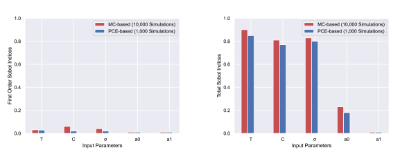
Figure 2: Larson-Miller model’s first-order (left) and total (right) Sobol indices.

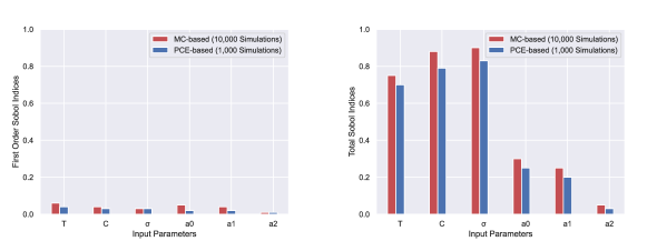
Figure 3: First-order (left) and total (right) Sobol indices for the Orr-Sherby-Dorn model.

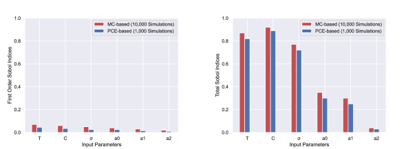
Figure 4: Manson-Succop model’s first-order (top) and total (bottm) Sobol indices.

4.3 Creep parameters’ probabilistic modeling

Following the global sensitivity analysis, the Central Limit Theorem was utilized to develop a probabilistic model for each parametric creep model’s most impactful parameters. These parameters were consequently modeled as jointly Gaussian. Their comprehensive probabilistic description is hence provided by the mean vector $\bm{\mu}$ and the covariance matrix $[\bm{\Sigma}]$.

The estimates for $\bm{\mu}$ and $[\bm{\Sigma}]$ were derived using the STLS method post the cross-validation process. For the Larson-Miller model, denoted as $\bm{X}=[a_{0},a_{1},C]^{T}$, the values were calculated as follows

$$\bm{\mu}^{\rm LM} = [26000,,-9.3,,23]^{T}\,,$$ (24)

$$\bm{\Sigma}^{\rm LM} = \begin{bmatrix}0.005&1.700&4.100\\ 1.700&0.070&1.400\\ 4.100&1.400&3.300\end{bmatrix}\times${10}^{-3}$\,.$$ (25)

For the Orr-Sherby-Dorn model ($\bm{X}=[a_{0},a_{1},a_{2},C]^{T}$), the results were

$$\bm{\mu}^{\rm OSD} = [-26.3,,-0.0016,,-0.000034,,21000]^{T}\,,$$ (26)

$$\bm{\Sigma}^{\rm OSD} = \begin{bmatrix}3.100&2.500&5.300&3.600\\ 2.500&170.000&48.000&820.000\\ 5.300&48.000&0.140&21.000\\ 3.600&820.000&21.000&0.004\end{bmatrix}\times${10}^{-3}$\,.$$ (27)

Lastly, for the Manson-Succop model ($\bm{X}=[a_{0},a_{1},a_{2},C]^{T}$), the outcomes were

$$\bm{\mu}^{\rm MS} = [24.8,-0.011,-0.000019,0.0289]^{T}\,,$$ (28)

$$\bm{\Sigma}^{\rm MS} = \begin{bmatrix}4.600&3.200&6.700&-3.600\\ 3.200&26.000&160.000&-35.000\\ 6.700&160.000&6.900&1.700\\ -3.600&-35.000&1.700&0.070\end{bmatrix}\times${10}^{-3}$\,.$$ (29)

4.4 Material rupture time: A statistical examination

Figures 5, 6, and 7 display the histograms derived from 10,000 sample points for the creep rupture time ($t_{r}$). The data was derived from a propagation of uncertainties in the input parameters for the Larson-Miller, Orr-Sherby-Dorn, and Manson-Succop creep parametric models. This was done under the four experimental conditions outlined in Table 4.

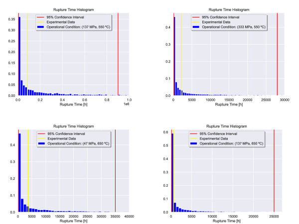
Figure 5: Rupture time histogram for Larson-Miller model for the four operational conditions.

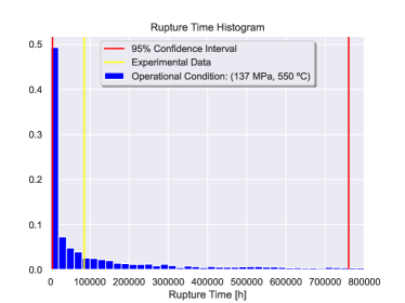
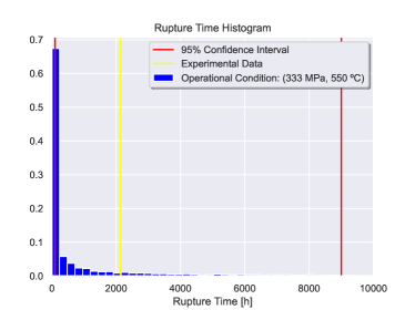
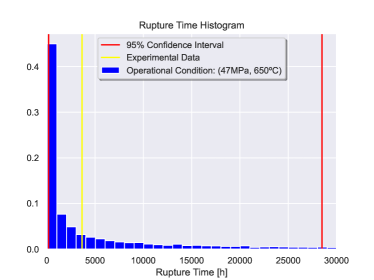
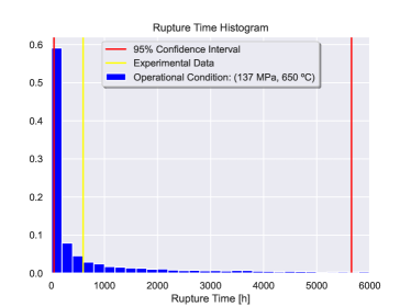
Figure 6: Rupture time histogram for Orr-Sherby-Dorn model for the four operational conditions.

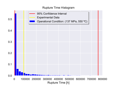
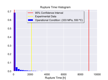
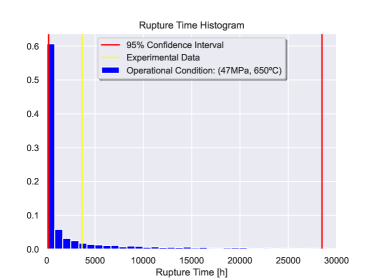
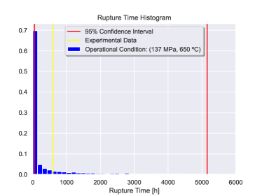
Figure 7: Rupture time histogram for Manson-Succop model for the four operational conditions.

Table 4: Experimental conditions applied in the study.

Condition	Stress [MPa]	Temperature [°C]
1	137	550
2	333	550
3	47	650
4	137	650

To grasp the inherent behavior of uncertainties surrounding the rupture time, we computed key statistical metrics: mean, standard deviation, skewness, kurtosis, and coefficient of variation. These metrics were calculated for each creep model under the four conditions detailed in Table 4. The results are compiled in Tables 5, 6, and 7.

Table 5: Calculated statistics for creep rupture time under the Larson-Miller parametric model for four experimental conditions as detailed in Table 4.

Condition	1	2	3	4
Mean	134,810h	1,774h	10,574h	106h
Standard deviation	337,025h	3,140h	21,888h	240h
Skewness	3.0	2.2	2.2	2.9
Kurtosis	9.2	4.2	4.2	8.7
Coefficient of variation	225%	177%	207%	219%

Table 6: Calculated statistics for creep rupture time under the Orr-Sherby-Dorn parametric model for four experimental conditions as detailed in Table 4.

Condition	1	2	3	4
Mean	103,986h	520h	9,915h	704h
Standard deviation	200,718h	1,585h	19,677h	1,650h
Skewness	2.4	4.3	2.6	3.2
Kurtosis	5.6	19.8	6.2	10.4
Coefficient of variation	190%	304%	198%	234%

Table 7: Calculated statistics for creep rupture time under the Manson-Succop parametric model for four experimental conditions as detailed in Table 4.

Condition	1	2	3	4
Mean	202,235h	2,694h	8,098h	691h
Standard deviation	410,148h	7,583h	18,079h	1,726h
Skewness	2.6	3.7	2.8	3.2
Kurtosis	6.0	14.5	7.9	10.2
Coefficient of variation	202%	280%	223%	249%

The histograms clearly demonstrate that the developed probabilistic models for creep rupture time cover the corresponding experimental measurements, as the measured creep rupture time (highlighted by yellow vertical lines in Figures 5, 6, and 7) resides within the 95% confidence interval computed with the probabilistic models (indicated by red vertical lines in Figures 5, 6, and 7).

The probabilistic models thus enhance the predictive accuracy of existing parametric models for creep life estimation, enriching the information extractable from these models. Notably, all creep parametric models show significant statistical dispersion for predicted creep rupture time. This outcome is affirmed by the nearly exponential probability distribution for creep rupture time, alongside the high values for the coefficient of variation (all exceeding 100%). This distribution aligns with the physics of creep phenomena, where thermal activation processes generally follow an Arrhenius exponential law. The mean creep rupture time varies significantly with operational condition, as anticipated, but intriguingly, its probability distribution seems unaffected by temperature and mechanical stress.

4.5 Identifying the optimal creep model

The appropriateness of the probabilistic model, where the mean value of creep rupture time closely mirrors the respective experimental value, varies depending on the specific experimental condition. For example, the Orr-Sherby-Dorn parametric model yielded the minimum relative error (1.5%) for experimental condition 2. Conversely, the Larson-Miller parametric model provided the smallest relative error (11%) for experimental condition 4. In general, the Orr-Sherby-Dorn parametric model proved to be more efficient at lower temperatures, as indicated by experimental conditions 1 and 2, despite displaying the most considerable dispersion (highest coefficient of variation) for experimental condition 2. Conversely, the Larson-Miller parametric model performed least effectively for operational conditions 3 and 4 (at higher temperatures), with experimental values of creep rupture time for these two conditions aligning closer to the lower limit of the 95% confidence interval calculated with the probabilistic Larson-Miller creep model. Hence, the probabilistic creep models exhibited superior performance under lower temperature conditions, a conclusion supported by a comparison of the relative errors between mean values and measured data.

The model selection outcomes are collated in Table 8, where the Akaike Information Criterion (AIC) and the Bayesian Information Criterion (BIC) are computed for the three probabilistic creep models studied in this research. It’s pertinent to note that the AIC and BIC values shown in Table 8 were computed by evaluating the likelihood function at the mean value $\bm{\mu}$.

Table 8: Calculated Akaike and Bayesian Information Criteria for the three probabilistic creep models.

Probabilistic Model	AIC	BIC
Larson-Miller	298.25	298.35
Orr-Sherby-Dorn	367.46	370.53
Manson-Succop	384.87	391.34

Both AIC and BIC scores were marginally lower for the three parametric creep models, which was expected as the Akaike criterion is less stringent in penalizing model complexity compared to the Bayesian criterion. The probabilistic Larson-Miller parametric model obtained the lowest values of both AIC and BIC. Its governing parameter (the Larson-Miller parameter) and mechanical stress maintain the simplest relationship (via an affine function). Conversely, the Orr-Sherby-Dorn and Manson-Succop parameters are quadratic functions of mechanical stress, adding complexity due to the increase in model parameters. Although the probabilistic Larson-Miller model is the least complex and exhibits superior predictive performance, it does not outperform the other two models significantly, as evidenced by the comparable AIC and BIC values obtained across all three probabilistic creep models.

5 Conclusion

This study introduces a probabilistic framework applied to the structural integrity of high-temperature metals subjected to the phenomenon of creep. It utilizes three well-established parametric models to predict creep rupture time, thereby demonstrating the utility of the framework.

An additional crucial contribution of this work is the enhancement of connections between probabilistic and statistical methods within the structural integrity community. This calls for a committed effort towards mastering probabilistic and statistical concepts and establishing a uniform understanding of these techniques within the community. The authors are optimistic that the broader dissemination of these methodologies will encourage their widespread adoption. This increased acceptance will foster more contributors, facilitating the maturity of this fresh perspective, thereby paving the way for the development of unified probabilistic frameworks to confront any structural integrity challenges.

Probabilistic methods should not be viewed as replacements for traditional deterministic methods. They should be considered a more comprehensive approach, introducing a fresh perspective on tackling structural integrity issues. Probabilistic methods can incorporate all model uncertainties without resorting to excessive conservatism due to gaps in knowledge. Hence, they can be seen as an extension beyond the conventional deterministic methods, which are commonly disseminated through statistical techniques and physical models for failure prevention, all the while being bolstered by advancements in scientific computation. A crucial aspect of applying a probabilistic framework to any structural integrity problem involves a deep understanding of the physics underlying the phenomena leading to structural deterioration, along with the information provided by observed data. Together, these two sources of information facilitate the creation of physically meaningful statistical models for both input parameters and output quantities associated with the structure’s reliability and integrity.

CRediT authorship contribution statement

VM: Conceptualization, Methodology, Software implementation, Data post-processing, Formal analysis, Investigation, Writing – original draft, Writing – review & editing. CFTM: Conceptualization, Methodology, Formal analysis, Fund acquisition, Supervision, Writing – review & editing. AC: Conceptualization, Methodology, Formal analysis, Fund acquisition, Supervision, Writing – review & editing.

Declaration of competing interest

The authors declare that they have no known competing financial interests or personal relationships that could have appeared to influence the work reported in this paper.

Disclaimer

This manuscript has undergone comprehensive grammatical review and enhancement using artificial intelligence-powered tools, including Grammarly and ChatGPT. However, the authors maintain full responsibility for the original language and wording.

References

- [1] M.-Y. Kim, D.-J. Chu, Y.-K. Lee, J.-H. Shim, W.-S. Jung, Residual lifetime assessment of cold-reheater pipe in coal-fired power plant through accelerated degradation test, Reliability Engineering & System Safety 188 (2019) 330–335. doi:10.1016/j.ress.2019.03.043.
- [2] R.-Z. Wang, H.-H. Gu, S.-P. Zhu, K.-S. Li, J. Wang, X.-W. Wang, M. Hideo, X.-C. Zhang, S.-T. Tu, A data-driven roadmap for creep-fatigue reliability assessment and its implementation in low-pressure turbine disk at elevated temperatures, Reliability Engineering & System Safety 225 (2022) 108523. doi:10.1016/j.ress.2022.108523.
- [3] N. E. Dowling, Mechanical Behavior of Materials, 4th Edition, Prentice Hall, 2012.
- [4] F. Dias, L. F. Paullo Muñoz, D. Roehl, A numerical model for basic creep of concrete with aging and damage on beams, Applied Mathematical Modelling 121 (2023) 185–203. doi:10.1016/j.apm.2023.04.018.
- [5] H.-F. Gao, Y.-H. Wang, Y. Li, E. Zio, Distributed-collaborative surrogate modeling approach for creep-fatigue reliability assessment of turbine blades considering multi-source uncertainty, Reliability Engineering & System Safety 250 (2024) 110316. doi:10.1016/j.ress.2024.110316.
- [6] R.-Z. Wang, H.-H. Gu, Y. Liu, H. Miura, X.-C. Zhang, S.-T. Tu, Surrogate-modeling-assisted creep-fatigue reliability assessment in a low-pressure turbine disc considering multi-source uncertainty, Reliability Engineering & System Safety 240 (2023) 109550. doi:10.1016/j.ress.2023.109550.
- [7] S. B. N. Roya, R. Ghoshc, Stochastic aspects of evolution of creep damage in austenitic stainless steel, Materials Science and Engineering A 527 (2010) 4810–4817. doi:10.1016/j.msea.2010.04.013.
- [8] V. T. Phan, X. Zhang, Y. Li, C. Oskay, Microscale modeling of creep deformation and rupture in nickel-based superalloy in 617 at high temperature, Mechanics of Materials 114 (2017) 215–227. doi:10.1016/j.mechmat.2017.08.008.
- [9] D. G. Harlow, T. J. Delph, A computational probabilistic model for creep-damaging solids, Computers & Structures 54 (1995) 161–166. doi:10.1016/0045-7949(94)E0253-X.
- [10] L. F. Fadel Miguel, A. T. Beck, Optimal path shape of friction-based Track-Nonlinear Energy Sinks to minimize lifecycle costs of buildings subjected to ground accelerations, Reliability Engineering & System Safety 248 (2024) 110172. doi:10.1016/j.ress.2024.110172.
- [11] W. J. S. Gomes, A. T. Beck, A conservatism index based on structural reliability and model errors, Reliability Engineering & System Safety 209 (2021) 107456. doi:10.1016/j.ress.2021.107456.
- [12] W. J. S. Gomes, A. T. Beck, T. Haukaas, Optimal inspection planning for onshore pipelines subject to external corrosion, Reliability Engineering & System Safety 118 (2013) 18–27. doi:10.1016/j.ress.2013.04.011.
- [13] B. S. Mohammad Lou, M. Pourgol-Mohamma, M. Yazdani, Probabilistic life assessment of gas turbine blade alloys under creep, International Journal of Reliability, Risk Safety: Theory and Application 3 (2020) 9–17. doi:10.30699/ijrrs.3.2.2.
- [14] J. Zhao, D. M. Li, J. S. Zhang, W. Feng, Y. Fang, Introduction of scri model for creep rupture life assessment, International Journal of Pressure Vessels and Piping 86 (2009) 599–603. doi:10.1016/j.ijpvp.2009.04.004.
- [15] M. A. Hossain, C. M. Stewart, A probabilistic creep model incorporating test condition, initial damage, and material property uncertainty, International Journal of Pressure Vessels and Piping 193 (2021) 104446. doi:10.1016/j.ijpvp.2021.104446.
- [16] A. T. Beck, L. A. Rodrigues da Silva, L. F. Fadel Miguel, The latent failure probability: A conceptual basis for robust, reliability-based and risk-based design optimization, Reliability Engineering & System Safety 233 (2023) 109127. doi:10.1016/j.ress.2023.109127.
- [17] F. Larson, J. Miller, A time-temperature relationship for rupture and creep stresses, Transactions of the American Society of Mechanical Engineers 74 (1952) 765–775.
- [18] B. K. Choudhary, W. G. Kim, M. D. Mathew, J. Jang, T. Jayakumar, Y. H. Jeong, On the reliability assessment of creep life for grade 91 steel, Procedia Engineering 86 (2014) 335–341. doi:10.1016/j.proeng.2014.11.046.
- [19] A. A. Ayubali, A. Singh, B. P. Shanmugavel, K. A. Padmanabhan, A phenomenological model for predicting long-term high temperature creep life of materials from short-term high temperature creep test data, International Journal of Mechanical Sciences 202-203 (2021) 106505. doi:10.1016/j.ijmecsci.2021.106505.
- [20] F. Monkman, N. Grant, An empirical relationship between rupture life and minimum creep rate in creep rupture tests, ASTM Proceedings 56 (1956) 593–620.
- [21] J. Gilbert, Z. Long, S. Ningileri, Application of Time-Temperature-Stress Parameters to High Temperature Performance of Aluminium Alloys, The Minerals, Metals & Materials Society, 2007.
- [22] R. Orr, O. Sherby, J. Dorn, Correlation of rupture data for metals at elevatnology, Institute of Engineering Research, Univ. of Calif., Berkeley (1954). doi:10.2172/4425999.
- [23] R. Carreker, Plastic flow of platinum wires., Journal of Applied Physics 21 (1950) 1289–1296. doi:10.1063/1.1699593.
- [24] A. Mullendore, J. Dhosi, N. Grant, Study of parameter techniques for the extrapolation of creep rupture properties, in conference proceedings 1963, Proceedings of the Institution of Mechanical Engineers (1963).
- [25] N. Allen, The extrapolation of creep tests, a review of recent opinion, Institute of Metals, London, UK (1960).
- [26] S. Manson, G. Succop, Stress-rupture properties of inconel 700 and correlation on the basis of several time-temperature parameters, ASTM STP (1956) 40–46.
- [27] N. Zharkova, L. Botvina, Estimate of the life of a material under creep conditions in the phase transition theory, ASTM 391 (2003) 334–336.
- [28] Z. Abdallah, K. Perkins, C. Arnold, Creep lifing models and techniques, in: T. A. Tański, M. Sroka, A. Zieliński (Eds.), Creep, IntechOpen, Chapter 7, 2018, pp. 115–149. doi:10.5772/intechopen.71826.
- [29] Z. Zhang, X. Wang, Z. Li, X. Xia, Y. Chen, T. Zhang, H. Zhang, Z. Yang, X. Zhang, J. Gong, Machine learning-assisted probabilistic creep life assessment for high-temperature superheater outlet header considering material uncertainty, International Journal of Pressure Vessels and Piping 209 (2024) 1–12. doi:10.1016/j.ijpvp.2024.105211.
- [30] A. Nispel, J. P. Dias, S. Ekwaro-Osire, A. Cunha Jr, Uncertainty quantification for fatigue life of offshore wind turbine structure, ASCE-ASME Journal of Risk and Uncertainty in Engineering Systems Part B: Mechanical Engineering 7 (2021) 040901. doi:10.1115/1.4051162.
- [31] J. P. Dias, S. Ekwaro-Osire, A. Cunha Jr, S. Dabetwar, A. Nispel, F. M. Alemayehu, H. B. Endeshaw, Parametric probabilistic approach for cumulative fatigue damage using double linear damage rule considering limited data, International Journal of Fatigue 127 (2019) 246–258. doi:10.1016/j.ijfatigue.2019.06.011.
- [32] J. P. Dias, S. Ekwaro-Osire, A. Cunha Jr, F. M. Alemayehu, S. Dabetwar, A. Nispel, A parametric probabilistic approach to quantify uncertainties in a non-linear cumulative fatigue damage model considering limited data, in: Twelfth International Conference on Fatigue Damage of Structural Materials (ICFDSM 2018), Hyannis, United States, 2018.
- [33] S. Boyd, L. Vandenberghe, Introduction to Applied Linear Algebra – Vectors, Matrices, and Least Squares, Cambridge University Press, 2018.
- [34] S. L. Brunton, J. L. Proctor, J. N. Kutz, Discovering governing equations from data by sparse identification of nonlinear dynamical systems, Proceedings of the National Academy of Sciences 113 (2016) 3932–3937. doi:10.1073/pnas.1517384113.
- [35] S. L. Brunton, J. N. Kutz, Data-Driven Science and Engineering: Machine Learning, Dynamical Systems, and Control, 2nd Edition, Cambridge University Press, 2022.
- [36] N. A. Zentuti, J. D. Booker, R. A. W. Bradford, A review of probabilistic techniques: towards developing a probabilistic lifetime methodology in the creep regime, Materials at High Temperatures 34 (2017) 333–341. doi:10.1080/09603409.2017.1371933.
- [37] B. Sudret, Global sensitivity analysis using polynomial chaos expansions, Reliability Engineering & System Safety 93 (7) (2008) 964–979. doi:10.1016/j.ress.2007.04.002.
- [38] D. P. Kroese, T. Taimre, Z. I. Botev, Handbook of Monte Carlo Methods, Wiley, 2011.
- [39] A. Cunha Jr, R. Nasser, R. Sampaio, H. Lopes, K. Breitman, Uncertainty quantification through Monte Carlo method in a cloud computing setting, Computer Physics Communications 185 (2014) 1355–1363. doi:10.1016/j.cpc.2014.01.006.
- [40] R. G. Ghanem, P. D. Spanos, Stochastic Finite Elements: A Spectral Approach, 2nd Edition, Dover Publications, 2003.
- [41] D. Xiu, Numerical Methods for Stochastic Computations: A Spectral Method Approach, Princeton University Press, 2010.
- [42] S. Marelli, B. Sudret, UQLab: a framework for uncertainty quantification in MATLAB, in: Proc. 2nd Int. Conf. on Vulnerability, Risk Analysis and Management (ICVRAM2014), Liverpool, United Kingdom, 2014, p. 2554–2563. doi:10.1061/9780784413609.257.
- [43] C. Soize, Uncertainty Quantification: An Accelerated Course with Advanced Applications in Computational Engineering, Springer, 2017.
- [44] A. C. Jr, Modeling and quantification of physical systems uncertainties in a probabilistic framework, in: S. Ekwaro-Osire, A. C. Gonçalves, F. M. Alemayehu (Eds.), Probabilistic Prognostics and Health Management of Energy Systems, Springer, Cham, 2017, pp. 127–156. doi:10.1007/978-3-319-55852-3_8.
- [45] R. C. Smith, Uncertainty Quantification: Theory, Implementation and Applications, SIAM, 2013.
- [46] L. Wasserman, All of Statistics: A Concise Course in Statistical Inference, Springer, 2004.
- [47] T. Hastie, R. Tibshirani, J. Friedman, The Elements of Statistical Learning, Springer, 2016.
- [48] K. P. Murphy, Machine Learning: A Probabilistic Perspective, The MIT Press, 2012.