Semantic Image Inversion and Editing using Rectified Stochastic Differential Equations

Abstract

Generative models transform random noise into images; their inversion aims to transform images back to structured noise for recovery and editing. This paper addresses two key tasks: (i) inversion and (ii) editing of a real image using stochastic equivalents of rectified flow models (such as Flux). Although Diffusion Models (DMs) have recently dominated the field of generative modeling for images, their inversion presents faithfulness and editability challenges due to nonlinearities in drift and diffusion. Existing state-of-the-art DM inversion approaches rely on training of additional parameters or test-time optimization of latent variables; both are expensive in practice. Rectified Flows (RFs) offer a promising alternative to diffusion models, yet their inversion has been underexplored. We propose RF inversion using dynamic optimal control derived via a linear quadratic regulator. We prove that the resulting vector field is equivalent to a rectified stochastic differential equation. Additionally, we extend our framework to design a stochastic sampler for Flux. Our inversion method allows for state-of-the-art performance in zero-shot inversion and editing, outperforming prior works in stroke-to-image synthesis and semantic image editing, with large-scale human evaluations confirming user preference.

Figure 1: Rectified flows for image inversion and editing. Our approach efficiently inverts reference style images in (a) and (b) without requiring text descriptions of the images and applies desired edits based on new prompts (e.g. “a girl” or “a dwarf”). For a reference content image (e.g. a cat in (c) or a face in (d)), it performs semantic image editing (e.g. “sleeping cat”) and stylization (e.g. “a photo of a cat in origmai style”) based on prompts, without leaking unwanted content from the reference image. Input images have orange borders.

1 Introduction

Vision generative models typically transform noise into images. Inverting such models, given a reference image, involves finding the structured noise that can regenerate the original image. Efficient inversion must satisfy two crucial properties. First, the structured noise should produce an image that is faithful to the reference image. Second, the resulting image should be easily editable using new prompts, allowing fine modifications over the image.

Diffusion Models (DMs) have become the mainstream approach for generative modeling of images (Sohl-Dickstein et al., 2015; Song & Ermon, 2019; Ho et al., 2020), excelling at sampling from high-dimensional distributions (Ramesh et al., 2021; Saharia et al., 2022; Ramesh et al., 2022; Rombach et al., 2022; Podell et al., 2023; Pernias et al., 2024). The sampling process follows a Stochastic Differential Equation known as reverse SDE (Anderson, 1982; Efron, 2011; Song et al., 2021b). Notably, these models can invert a given image. Recent advances in DM inversion have shown a significant impact on conditional sampling, such as stroke-to-image synthesis (Meng et al., 2022), image editing (Hertz et al., 2022; Mokady et al., 2023; Couairon et al., 2023; Rout et al., 2023a; b; 2024a; Delbracio & Milanfar, 2023) and stylization (Hertz et al., 2023; Rout et al., 2024b).

Despite its widespread usage, DM inversion faces critical challenges in faithfulness and editability. First, the stochastic nature of the process requires fine discretization of the reverse SDE (Ho et al., 2020; Song et al., 2021b), which increases expensive Neural Function Evaluations (NFEs). Coarse discretization, on the other hand, leads to less faithful outputs (Meng et al., 2022), even with deterministic methods like DDIM (Song et al., 2021a; b). Second, nonlinearities in the reverse trajectory introduce unwanted drift, reducing the accuracy of reconstruction (Karras et al., 2024). While existing methods enhance faithfulness by optimizing latent variables (Rout et al., 2024a) or prompt embeddings (Mokady et al., 2023; Miyake et al., 2023), they tend to be less efficient, harder to edit, and rely on complex attention processors to align with a given prompt (Hertz et al., 2022; Rout et al., 2024a). These added complexities make such methods less suitable for real-world deployment.

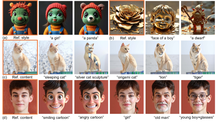
For inversion and editing, we introduce a zero-shot conditional sampling algorithm using Rectified Flows (RFs) (Liu et al., 2022; Albergo & Vanden-Eijnden, 2023; Lipman et al., 2022; Esser et al., 2024), a powerful alternative to DMs. Unlike DMs, where sampling is governed by a reverse SDE, RFs use an Ordinary Differential Equation known as reverse ODE, offering advantages in both efficient training and fast sampling. We construct a controlled forward ODE, initialized from a given image, to generate the initial conditions for the reverse ODE. The reverse ODE is then guided by an optimal controller, obtained through solving a Linear Quadratic Regulator (LQR) problem. We prove that the resulting new vector fields have a stochastic interpretation with an appropriate drift and diffusion. We evaluate RF inversion on stroke-to-image generation and image editing tasks, and show extensive qualitative results on other applications like cartoonization. Our method significantly improves photo realism in stroke-to-image generation, surpassing a state-of-the-art (SoTA) method (Mokady et al., 2023) by 89%, while maintaining faithfulness to the input stroke. In addition, we show that RF inversion outperforms DM inversion (Meng et al., 2022) in faithfulness by 4.7% and in realism by 13.8% on LSUN-bedroom dataset (Wang et al., 2017). Figure 1 and Figure 2 show the qualitative results of our approach and a graphical illustration, respectively.

Our theoretical and practical contributions can be summarized as:

• We present an efficient inversion method for RF models, including Flux, that requires no additional training, latent optimization, prompt tuning, or complex attention processors.

• We develop a new vector field for RF inversion, interpolating between two competing objectives: consistency with a possibly corrupted input image, and consistency with the “true” distribution of clean images (§3.3). We prove that this vector field is equivalent to a rectified SDE that interpolates between the stochastic equivalents of these competing objectives (§3.4). We extend the theoretical results to design a stochastic sampler for Flux.

• We demonstrate the faithfulness and editability of RF inversion across three benchmarks: (i) LSUN-Bedroom, (ii) LSUN-Church, and (iii) SFHQ, on two tasks: stroke-to-image synthesis and image editing. In addition, we provide extensive qualitative results and conduct large-scale human evaluations to assess user preference metrics (§5).

[capbesideposition=left,top,capbesidewidth=0.6]figure[]

Figure 2: Graphical model illustrating (a) DDIM inversion and (b) RF inversion. Due to nonlinearities in DM trajectory, the DDIM inverted latent ${\mathbf{x}}_{1}$ significantly deviates from the original image ${\mathbf{y}}_{0}$. RF inversion without controller reduces this deviation, resulting in ${\mathbf{x}}_{1}$. With controller, RF inversion further eliminates the reconstruction error, making ${\mathbf{x}}_{1}$ nearly identical to ${\mathbf{y}}_{0}$, which enhances the faithfulness.

2 Related Works

DM Inversion. Diffusion models have become the mainstream approach for generative modeling, making DM inversion an exciting area of research (Meng et al., 2022; Couairon et al., 2023; Song et al., 2021b; Hertz et al., 2023; Mokady et al., 2023; Rout et al., 2024a). Among training-free methods, SDEdit (Meng et al., 2022) adds noise to an image and uses the noisy latent as structured noise. For semantic image editing based on a given prompt, it simulates the standard reverse SDE starting from this structured noise. SDEdit requires no additional parameter training, latent variable optimization, or complex attention mechanisms. However, it is less faithful to the original image because adding noise in one step is equivalent to linear interpolation between the image and noise, while the standard reverse SDE follows a nonlinear path (Liu et al., 2022; Karras et al., 2022).

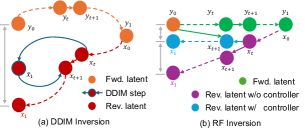
An alternate method, DDIM inversion (Song et al., 2021a; b), recursively adds predicted noise at each forward step and returns the final state as the structured noise (illustrated by $Y_{t}$ process in Figure 2(a)). However, DDIM inversion often deviates significantly from the original image due to nonlinearities in the drift and diffusion coefficients, as well as inexact score estimates (Mokady et al., 2023). To reduce this deviation, recent approaches optimize prompt embeddings (Mokady et al., 2023) or latent variables (Rout et al., 2024a), but they have high time complexity. Negative prompt inversion (Miyake et al., 2023) speeds up the inversion process but sacrifices faithfulness. Methods like CycleDiffusion (Wu & De la Torre, 2023) and Direction Inversion (Ju et al., 2023) use inverted latents as references during editing, but they are either computationally expensive or not applicable to rectified flow models like Flux or SD3 (Esser et al., 2024).

DM Editing. Efficient inversion is crucial for real image editing. Once a structured noise is obtained by inverting the image, a new prompt is fed into the T2I generative model. Inefficient inversion often fails to preserve the original content and therefore requires complex editing algorithms. These editing algorithms can be broadly classified into (i) attention control, such as prompt-to-prompt (Hertz et al., 2022), plug-and-play (PnP) (Tumanyan et al., 2023), (ii) optimization-based methods like DiffusionCLIP (Kim et al., 2022), DiffuseIT (Kwon & Ye, 2023), STSL (Rout et al., 2024a), and (iii) latent masking to edit specific regions of an image using masks provided by the user (Nichol et al., 2022) or automatically extracted from the generative model (Couairon et al., 2023). We focus on efficient inversion, avoiding the need for complex editing algorithms.

Challenges in RF Inversion. Previous inversion or editing approaches have been tailored towards diffusion models and do not directly apply to SoTA rectified flow models like Flux. This limitation arises because the network architecture of Flux is MM-DiT (Peebles & Xie, 2023), which is fundamentally different from the traditional UNet used in DMs (Ho et al., 2020; Song et al., 2021a; b). In MM-DiT, text and image information are entangled within the architecture itself, whereas in UNet, text conditioning is handled via cross-attention layers. Additionally, Flux primarily uses T5 text encoder, which lacks an aligned latent space for images, unlike CLIP encoders. Therefore, extending these prior methods to modern T2I generative models requires a thorough investigation. We take the first step by inverting and editing a given image using Flux.

RF Inversion and Editing. DMs (Ho et al., 2020; Song et al., 2021a; Rombach et al., 2022) traditionally outperform RFs (Lipman et al., 2022; Liu et al., 2022; Albergo & Vanden-Eijnden, 2023) in high-resolution image generation. However, recent advances have shown that RF models like Flux can surpass SoTA DMs in text-to-image (T2I) generation tasks (Esser et al., 2024). Despite this, their inversion and editing capabilities remain underexplored. In this paper, we introduce an efficient RF inversion method that avoids the need for training additional parameters (Hu et al., 2021; Ruiz et al., 2023), optimizing latent variables (Rout et al., 2024a), prompt tuning (Mokady et al., 2023), or using complex attention processors (Hertz et al., 2022). While our focus is on inversion and editing, we also show that our framework can be easily extended to generative modeling.

Filtering, Control and SDEs. There is a rich literature on the connections between nonlinear filtering, optimal control and SDEs (Fleming & Rishel, 1975; Øksendal, 2003; Tzen & Raginsky, 2019; Zhang & Chen, 2022). These connections are grounded in the Fokker-Planck equation (Øksendal, 2003), which RF methods (Lipman et al., 2022; Liu et al., 2022; Albergo & Vanden-Eijnden, 2023; Albergo et al., 2023) heavily exploit in sampling. Our study focuses on rectified flows for conditional sampling, and shows that the resulting drift field also has an optimal control interpretation.

3 Method

3.1 Preliminaries

In generative modeling, the goal is to sample from a target distribution $p_{0}$ given a finite number of samples from that distribution. Rectified flows (Lipman et al., 2022; Liu et al., 2022) represent a class of generative models that construct a source distribution $q_{0}$ and a time varying vector field $v_{t}({\mathbf{x}}_{t})$ to sample $p_{0}$ using an ODE:

$$\mathrm{d}X_{t}=v_{t}(X_{t})\mathrm{d}t,\quad X_{0}\sim q_{0},\quad t\in[0,1].$$ (1)

Starting from $X_{0}={\mathbf{x}}_{0}$, the ODE (1) is integrated from $t:0\rightarrow 1$ to yield a sample ${\mathbf{x}}_{1}$ distributed according to $p_{0}$ (e.g., the distribution over images). A common choice of $q_{0}$ is standard Gaussian ${\mathcal{N}}\left(0,I\right)$ and $v_{t}\left(X_{t}\right)=-u(X_{t},1-t;\varphi)$, where $u$ is a neural network parameterized by $\varphi$. The neural network is trained using the conditional flow matching objective as discussed below.

Training Rectified Flows. To train a neural network to serve as the vector field for the ODE (1), we couple samples from $p_{0}$ with samples from $q_{0}$ – which we call $p_{1}$ to simplify the notation – via a linear path: $Y_{t}=tY_{1}+(1-t)Y_{0}$. The resulting marginal distribution of $Y_{t}$ becomes:

$$p_{t}({\mathbf{y}}_{t})=\mathbb{E}_{Y_{1}\sim p_{1}}\left[p_{t}({\mathbf{y}}_{t}|Y_{1})\right]=\int p_{t}({\mathbf{y}}_{t}|{\mathbf{y}}_{1})p_{1}({\mathbf{y}}_{1})\mathrm{d}{\mathbf{y}}_{1}.$$ (2)

Given an initial state $Y_{0}={\mathbf{y}}_{0}$ and a terminal state $Y_{1}={\mathbf{y}}_{1}$, the linear path induces an ODE: $\mathrm{d}Y_{t}=u_{t}\left(Y_{t}|{\mathbf{y}}_{1}\right)\mathrm{d}t$ with the conditional vector field $u_{t}\left(Y_{t}|{\mathbf{y}}_{1}\right)={\mathbf{y}}_{1}-{\mathbf{y}}_{0}$. The marginal vector field is derived from the conditional vector field using the following relation (Lipman et al., 2022):

$$u_{t}({\mathbf{y}}_{t})=\mathbb{E}_{Y_{1}\sim p_{1}}\left[u_{t}\left({\mathbf{y}}_{t}|Y_{1}\right)\frac{p_{t}({\mathbf{y}}_{t}|Y_{1})}{p_{t}({\mathbf{y}}_{t})}\right]=\int u_{t}\left({\mathbf{y}}_{t}|{\mathbf{y}}_{1}\right)\frac{p_{t}({\mathbf{y}}_{t}|{\mathbf{y}}_{1})}{p_{t}({\mathbf{y}}_{t})}p_{1}({\mathbf{y}}_{1})\mathrm{d}{\mathbf{y}}_{1}.$$ (3)

We can then use a neural network $u({\mathbf{y}}_{t},t;\varphi)$, parameterized by $\varphi$, to approximate the marginal vector field $u_{t}({\mathbf{y}}_{t})$ through the flow matching objective defined as:

$${\mathcal{L}}_{FM}(\varphi)\coloneqq\mathbb{E}_{t\sim{\mathcal{U}}[0,1],Y_{t}\sim p_{t}}\left[\left\|u_{t}(Y_{t})-u(Y_{t},t;\varphi)\right\|_{2}^{2}\right].$$ (4)

For tractability, we can instead consider a different objective, called conditional flow matching:

$${\mathcal{L}}_{CFM}(\varphi)\coloneqq\mathbb{E}_{t\sim{\mathcal{U}}[0,1],Y_{t}\sim p_{t}(\cdot|Y_{1}),Y_{1}\sim p_{1}}\left[\left\|u_{t}(Y_{t}|Y_{1})-u(Y_{t},t;\varphi)\right\|_{2}^{2}\right].$$ (5)

${\mathcal{L}}_{CFM}$ and ${\mathcal{L}}_{FM}$ have the identical gradients (Lipman et al., 2022, Theorem 2), and are hence equivalent. However, ${\mathcal{L}}_{CFM}(\varphi)$ is computationally tractable, unlike ${\mathcal{L}}_{FM}(\varphi)$, and therefore preferred during training. Finally, the required vector field in (1) is computed as $v_{t}\left(X_{t}\right)=-u(X_{t},1-t;\varphi)$. In this way, rectified flows sample a data distribution by an ODE with a learned vector field.

3.2 Connection between Rectified Flows and Linear Quadratic Regulator

The unconditional rectified flows (RFs) (e.g., Flux) from Section §3.1 above, enable image generation by simulating the vector field $v_{t}(\cdot)$ initialized with a sample of random noise. Subsequently, by simulating the reversed vector field $-v_{1-t}(\cdot)$ starting from the image, we get back the sample of noise that we started with. We formalize this statement below.

Proposition 3.1.

Given an image ${\mathbf{y}}_{0}$ and the vector field $v_{t}(\cdot)$ of the generative ODE (1), suppose the structured noise ${\mathbf{y}}_{1}$ is obtained by simulating an ODE:

$$\mathrm{d}Y_{t}=u_{t}(Y_{t})\mathrm{d}t,\quad Y_{0}={\mathbf{y}}_{0},\quad t\in[0,1].$$ (6)

If $u_{t}(\cdot)=-v_{1-t}(\cdot)$ and $X_{0}={\mathbf{y}}_{1}$, then the ODE (1) recovers the original image, i.e., $X_{1}={\mathbf{y}}_{0}$.

Implication. Rectified flows enable exact inversion of a given image when the vector field of the generative ODE (1) is precisely known. Employing ODE (6) for the structured noise and ODE (1) to transform that noise back into an image, RF inversion accurately recovers the given image.

Suppose instead that we start with a corrupted image and simulate the reversed vector field $-v_{1-t}(\cdot)$. Then we obtain a noise sample. There are two salient aspects of this noise sample. First, it is consistent with the original image: when processed through $v_{t}(\cdot)$ it results in the same corrupted image. Second, if the image sample is “atypical” (e.g., corrupted, or, say, a stroke painting as in §5), then the sample of noise is also likely to be atypical. In other words, the noise sample is only consistent to the (possibly corrupted) image sample.

Our goal is to modify the pipeline above so that even when we start with a corrupted image, we can get back a clean image (see stroke-to-image synthesis in  Figure 5), but for this, we need to processs by $v_{t}(\cdot)$ a noise sample that is closer to being “typical”. More generally, the goal is to create a pipeline that supports semantic editing of real images (§5), e.g., changing age, or gender without relying on additional training, optimization, or complex attention processors.

Thus, as a first step, we derive an optimal controller that takes a minimum energy path to convert any image $Y_{0}$ (whether corrupted or not) to a given sample of random noise $Y_{1}\sim p_{1}$ – i.e., noise that is typical for $p_{1}$. Specifically, we consider optimal control in a $d$-dimensional vector space $\mathbb{R}^{d}$:

$$V(c)\coloneqq\int_{0}^{1}\frac{1}{2}\left\|c\left(Z_{t},t\right)\right\|_{2}^{2}\mathrm{d}t+\frac{\lambda}{2}\left\|Z_{1}-Y_{1}\right\|_{2}^{2},~{}\mathrm{d}Z_{t}=c\left(Z_{t},t\right)\mathrm{d}t,~{}Z_{0}={\mathbf{y}}_{0},~{}Y_{1}\sim p_{1},$$ (7)

where $\lambda$ is the weight assigned to the terminal cost and $V(c)$ denotes the total cost of the control $c:\mathbb{R}^{d}\times[0,1]\rightarrow\mathbb{R}^{d}$. The minimization of $V(c)$ over the admissible set of controls, denoted by ${\mathcal{C}}$, is known as the Linear Quadratic Regulator (LQR) problem. The solution of the LQR problem (7) is given in Proposition 3.2, which minimizes the quadratic transport cost of the dynamical system.

Proposition 3.2.

For $Z_{0}={\mathbf{y}}_{0}$ and $Y_{1}={\mathbf{y}}_{1}$, the optimal controller of the LQR problem (7), denoted by $c^{*}\left(\cdot,t\right)$ is equal to the conditional vector field $u_{t}\left(\cdot|{\mathbf{y}}_{1}\right)$ of the rectified linear path $Y_{t}=tY_{1}+(1-t)Y_{0}$ when $Y_{0}={\mathbf{y}}_{0}$, i.e., $c^{*}\left({\mathbf{z}}_{t},t\right)=u_{t}\left({\mathbf{z}}_{t}|{\mathbf{y}}_{1}\right)=({\mathbf{y}}_{1}-{\mathbf{z}}_{t})/(1-t)$.

3.3 Inverting Rectified Flows With Dynamic Control

So far, we have two vector fields. The first, from the RFs, transforms an image $Y_{0}$ typical for distribution $p_{0}$ to a typical sample of random Gaussian noise $Y_{1}\sim p_{1}.$ As discussed above, if the image sample is atypical, then the sample of noise is also likely to be atypical.

We also have a second vector field resulting from the optimal control formulation that transforms any image (whether corrupted or not) to a noise sample that is typical-by-design from the distribution $p_{1}$. Therefore, this sample, when passed through the rectified flow ODE (1) results in a “typical” image from the “true” distribution $p_{0}$. This image is clean, i.e., typical for $p_{0}$, but it is not related to the image $Y_{0}$. Our controlled ODE, defined below, interpolates between these two differing objectives – consistency with the given (possibly corrupted) image, and consistency with the distribution of images $p_{0}$ – with a tunable parameter $\gamma$:

$$\mathrm{d}Y_{t}=\Big{[}u_{t}(Y_{t})+\gamma\left(u_{t}(Y_{t}|{\mathbf{y}}_{1})-u_{t}(Y_{t})\right)\Big{]}\mathrm{d}t,\quad Y_{0}={\mathbf{y}}_{0},$$ (8)

where $u_{t}(Y_{t}|{\mathbf{y}}_{1})=c^{*}(Y_{t},t)$ is computed based on the insights from Proposition 3.2, and $u_{t}(Y_{t})=-v_{1-t}(Y_{t})$ as established in Proposition 3.1. Here, we call $\gamma\in[0,1]$ the controller guidance. Thus, ODE (8) generalizes (6) to editing applications, while keeping its inversion accuracy comparable.

When $\gamma=1$, the drift field of the ODE (8) becomes optimal controller of LQR problem (7), ensuring that the structured noise $Y_{1}={\mathbf{y}}_{1}$ adheres to the distribution $p_{1}$. Consequently, initializing the generative ODE (1) with ${\mathbf{y}}_{1}$ results in samples with high likelihood under the data distribution $p_{0}$.

Conversely, when $\gamma=0$, the system follows the ODE (6) described in Proposition 3.1, resulting a structured noise $Y_{1}$ that is not guaranteed to follow the noise distribution $p_{1}$. However, initializing the generative ODE (1) with this noise precisely recovers the reference image ${\mathbf{y}}_{0}$.

Beyond this vector field interpolation intuition, we show in the next section §3.4 that the controlled ODE (8) has an SDE interpretation. As is well known (Ho et al., 2020; Song et al., 2021a; Meng et al., 2022; Song et al., 2021b), SDEs are robust to initial conditions, in proportion to the variance of the additive noise. Specifically, errors propagate over time in an ODE initialized with an incorrect or corrupted sample. However, SDEs (Markov processes) under appropriate conditions converge to samples from a carefully constructed invariant distribution with reduced sensitivity to the initial condition, resulting in a form of robustness to initialization. As we see, the parameter $\gamma$ (the controller guidance) appears in the noise term to the SDE, thus the SDE analysis in the next section again provides intuition on the trade-off between consistency to the (corrupted) image and consistency to the terminal invariant distribution.

Remark 3.3.

We note that our analysis extends to the case where $\gamma$ is time-varying, though we omit these results for simplicity of notation. This is useful in practice, especially when ${\mathbf{y}}_{0}$ is a corrupted image, because for large $\gamma$ the stochastic evolution (22) moves toward a sample from the invariant measure ${\mathcal{N}}\left(0,I\right)$. This noise encodes clean images. Starting from this noise, the corresponding reverse process operates in pure diffusion mode, resulting in a clean image. As the process approaches the terminal state, $\gamma$ is gradually reduced to ensure that ${\mathbf{y}}_{0}$ is encoded through $u_{t}(\cdot)$ into the final structured noise sample.

3.4 Controlled Rectified Flows as Stochastic Differential Equations

An SDE (Ho et al., 2020) is known to have an equivalent ODE formulation (Song et al., 2021a) under certain regularity conditions (Anderson, 1982; Song et al., 2021b). In this section, we derive the opposite: an SDE formulation for our controlled ODE (8) from §3.3. Let $W_{t}$ be a $d$-dimensional Brownian motion in a filtered probability space $(\Omega,{\mathcal{F}},\{{\mathcal{F}}_{t}\},\mathbb{P})$.

Theorem 3.4.

Fix any $T\in(0,1)$. For any $t\in[0,T]$, the controlled ODE (8) is explicitly given by:

$$\mathrm{d}Y_{t}=\left[-\frac{1}{1-t}\left(Y_{t}-\gamma{\mathbf{y}}_{1}\right)-\frac{(1-\gamma)t}{1-t}\nabla\log p_{t}(Y_{t})\right]\mathrm{d}t,\quad Y_{0}\sim p_{0}.$$ (9)

Its density evolution is identical to the density evolution of the following SDE:

$$\mathrm{d}Y_{t}=-\frac{1}{1-t}\left(Y_{t}-\gamma{\mathbf{y}}_{1}\right)\mathrm{d}t+\sqrt{\frac{2(1-\gamma)t}{1-t}}\mathrm{d}W_{t},\quad Y_{0}\sim p_{0}.$$ (10)

Finally, denoting $p_{t}(\cdot)$ as the marginal pdf of $Y_{t}$, the density evolution is explicitly given by:

$$\frac{\partial p_{t}(Y_{t})}{\partial t}=\nabla\cdot\left[\left(\frac{1}{1-t}\left(Y_{t}-\gamma{\mathbf{y}}_{1}\right)+\frac{(1-\gamma)t}{1-t}\nabla\log p_{t}(Y_{t})\right)p_{t}(Y_{t})\right].$$ (11)

Properties of SDE (10). Elaborating on the intuition discussed at the end of §3.3, when the controller guidance parameter $\gamma=0$, it becomes the stochastic equivalent of the standard RFs; see Lemma A.2 for a precise statement. The resulting SDE is given by

$$\mathrm{d}Y_{t}=-\frac{1}{1-t}Y_{t}\mathrm{d}t+\sqrt{\frac{2t}{1-t}}\mathrm{d}W_{t},\quad Y_{0}\sim p_{0},$$ (12)

which improves faithfulness to the image $Y_{0}$. When $\gamma=1$, the SDE (10) solves the LQR problem (7) and drives towards the terminal state $Y_{1}={\mathbf{y}}_{1}$. This improves the generation quality, because the sample $Y_{1}$ is from the correct noise distribution $p_{1}$ as previously discussed in §3.3. Therefore, a suitable choice of $\gamma$ retains faithfulness while simultaneously applying the desired edits.

Finally, we assume $T=1-\delta$ for sufficiently small $\delta$ (such that $0<\delta\ll 1$) to avoid irregularities at the boundary. This is typically considered in practice for numerical stability (even for diffusion models). Thus, in practice, the final sample ${\mathbf{y}}_{1-\delta}$ is returned as ${\mathbf{y}}_{1}$.

Comparison with DMs. Analogous to the SDE (12), the stochastic noising process of DMs is typically modeled by the Ornstein-Uhlenbeck (OU) process, governed by the following SDE:

$$\mathrm{d}Y_{t}=-Y_{t}\mathrm{d}t+\sqrt{2}\mathrm{d}W_{t}.$$ (13)

The corresponding ODE formulation is given by:

$$\mathrm{d}Y_{t}=\left[-Y_{t}-\nabla\log p_{t}(Y_{t})\right]\mathrm{d}t.$$ (14)

Instead, our approach is based on rectified flows (1), which leads to a different ODE and consequently translates into a different SDE. As an additional result, we formalize the ODE derivation in Lemma A.1. In Lemma A.2, we show that the marginal distribution of this ODE is equal to that of an SDE with appropriate drift and diffusion terms. In Proposition A.3, we show that the stationary distribution of this new SDE (12) converges to the standard Gaussian ${\mathcal{N}}(0,I)$ in the limit as $t\rightarrow 1$.

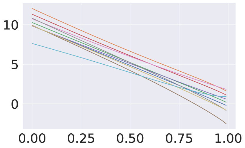
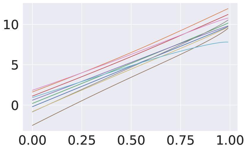
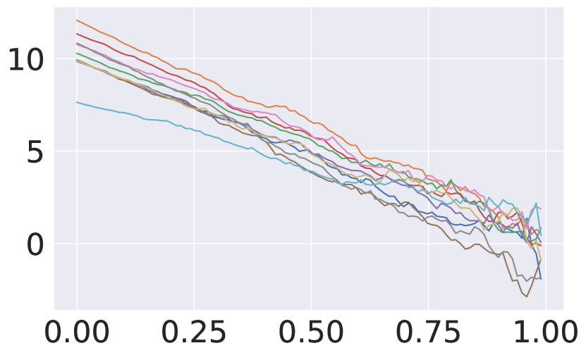
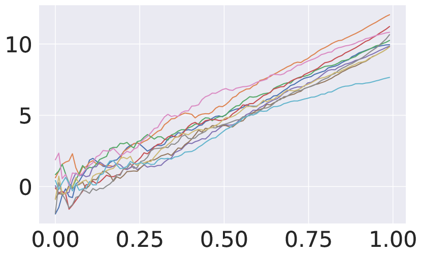
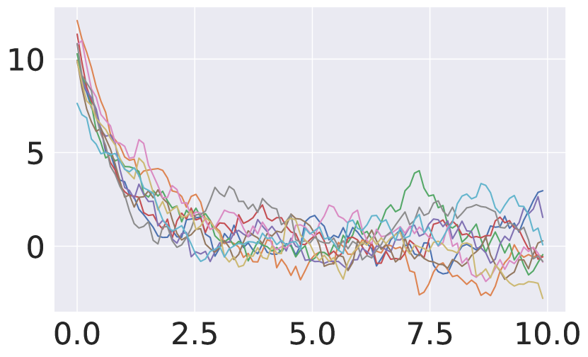
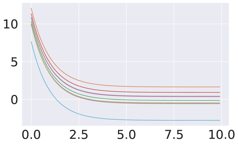
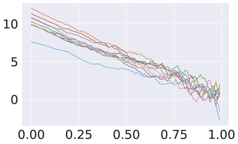
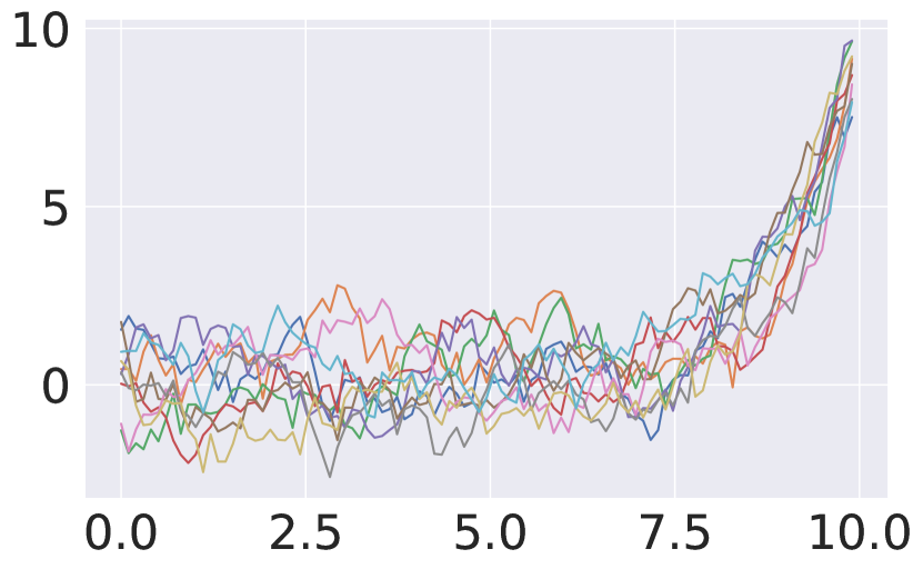
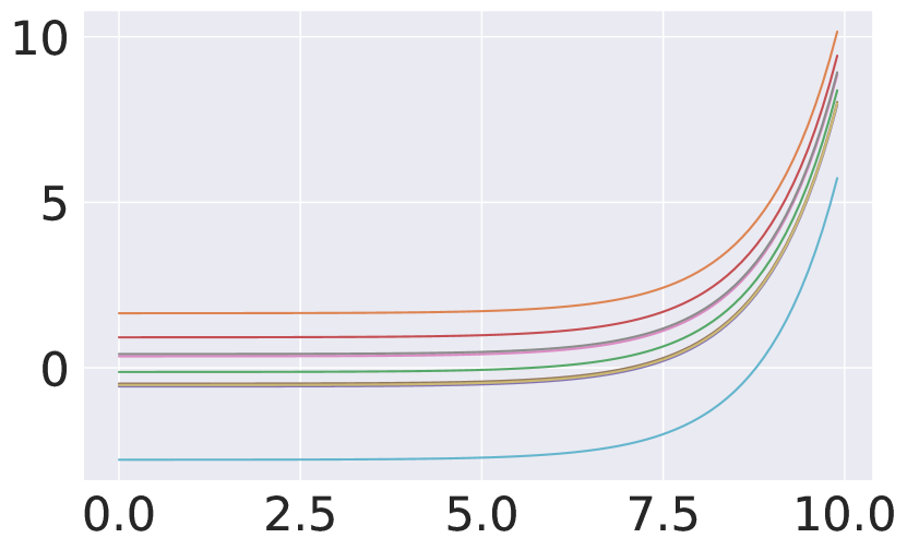
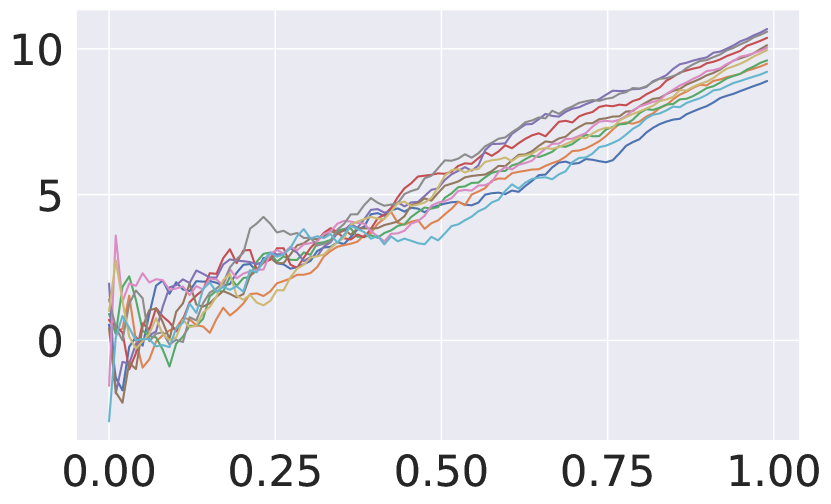
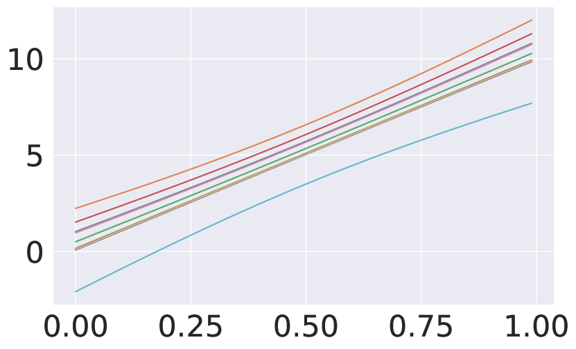
The standard OU process (13) interpolates between the data distribution at time $t=0$ and a standard Gaussian as $t\to\infty$. The SDE (12), however, interpolates between the data distribution at time $t=0$ and a standard Gaussian at $t=1$. In other words, it effectively “accelerates” time as it progresses to achieve the terminal Gaussian distribution. This is accomplished by modifying the coefficients of drift and diffusion as in (12) to depend explicitly on time $t$. Thus, a sample path of (12) appears like a noisy line, unlike that of the OU process (see Appendix C.3 for numerical simulations).

3.5 Controlled Reverse Flow using Rectified ODEs and SDEs

In this section, we develop an ODE and an SDE similar to our discussions above, but for the reverse direction (i.e., from noise to images).

Reverse process using ODE. Starting from the structured noise ${\mathbf{y}}_{1}$ obtained by integrating the controlled ODE (8), we construct another controlled ODE (15) for the reverse process (i.e., noise to image). In this process, the optimal controller uses the reference image ${\mathbf{y}}_{0}$ for guidance:

$$\mathrm{d}X_{t}=\Big{[}v_{t}(X_{t})+\eta\left(v_{t}(X_{t}|{\mathbf{y}}_{0})-v_{t}(X_{t})\right)\Big{]}\mathrm{d}t,\quad X_{0}={\mathbf{y}}_{1},\quad t\in[0,1],$$ (15)

where $\eta\!\in\![0,1]$ is the controller guidance parameter as before that controls faithfulness and editability of the given image ${\mathbf{y}}_{0}$. Similar to the analysis in Proposition 3.2, $v_{t}(X_{t}|{\mathbf{y}}_{0})$ is obtained by solving the modified LQR problem (16):

$$V(c)=\int_{0}^{1}\frac{1}{2}\left\|c\left(Z_{t},t\right)\right\|_{2}^{2}\mathrm{d}t+\frac{\lambda}{2}\left\|Z_{1}-{\mathbf{y}}_{0}\right\|_{2}^{2},~{}\mathrm{d}Z_{t}=c\left(Z_{t},t\right)\mathrm{d}t,\quad Z_{0}={\mathbf{y}}_{1}.$$ (16)

Solving (16), we get $c(Z_{t},t)=\frac{{\mathbf{y}}_{0}-Z_{t}}{1-t}$. Our controller steers the samples toward the given image ${\mathbf{y}}_{0}$. Thus, the controlled reverse ODE (15) effectively reduces the reconstruction error incurred in the standard reverse ODE (1) of RF models (e.g. Flux).

Reverse process using SDE. Finally, in Theorem 3.5, we provide the stochastic equivalent of our controlled reverse ODE (15) for generation. Recall that we initialize with the terminal structured noise by running the controlled forward ODE (8), along with a reference image ${\mathbf{y}}_{0}$. As discussed above, we terminate the inversion process at a time $T=1-\delta$ for numerical stability, resulting in a vector ${\mathbf{y}}_{1-\delta}$. Our reverse SDE thus starts at a corresponding time $\delta$ with this vector ${\mathbf{y}}_{1-\delta}$ at initialization, and terminates at time $T^{\prime}<1.$

Theorem 3.5.

Fix any $T^{\prime}\in(\delta,1)$, and for any $t\in[\delta,T^{\prime}]$, the density evolution of the controlled ODE (15) initialized at $X_{0}={\mathbf{y}}_{1-\delta}$ is identical to the density evolution of the following SDE:

$$\mathrm{d}X_{t}=\left[\frac{(1-t-\eta)X_{t}+\eta t{\mathbf{y}}_{0}}{t(1-t)}+\frac{2(1-t)(1-\eta)}{t}\nabla\log p_{1-t}(X_{t})\right]\mathrm{d}t+\sqrt{\frac{2(1-t)(1-\eta)}{t}}\mathrm{d}W_{t}.$$ (17)

Furthermore, denoting $q_{t}(\cdot)$ as the marginal pdf of $X_{t}$, its density evolution is given by:

$$\frac{\partial q_{t}(X_{t})}{\partial t}=\nabla\cdot\left[-\left(\frac{1-t-\eta}{t(1-t)}X_{t}+\frac{\eta}{1-t}{\mathbf{y}}_{0}+\frac{(1-t)}{t}(1-\eta)\nabla\log p_{1-t}(X_{t})\right)q_{t}(Y_{t})\right].$$ (18)

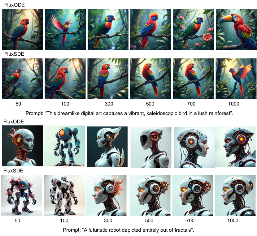
Properties of SDE (17). When the controller parameter $\eta=0$, we obtain a stochastic sampler (22) for the pre-trained Flux, as given in Lemma A.4 and compared qualitatively in Figure 24. This case of our SDE (17) corresponds to the stochastic variant of standard RFs (Liu et al., 2022; Lipman et al., 2022; Albergo & Vanden-Eijnden, 2023). Our key contribution lies in conditioning on $X_{1}={\mathbf{y}}_{0}$ for inverting rectified flows. Importantly, our explicit construction does not require additional training or test-time optimization, enabling for the first time an efficient sampler for zero-shot inversion and editing using Flux. When $\eta=1$, the score term and Brownian motion vanish from the SDE (17). The resulting drift becomes $\frac{{\mathbf{y}}_{0}-X_{t}}{1-t}$, the optimal controller for the LQR problem (16), exactly recovering the given image ${\mathbf{y}}_{0}$.

Remark 3.6.

Similar to Remark 3.3, our analysis extends to the case when $\eta$ is time-varying. This is useful in editing, as it allows the flow to initially move toward the given image ${\mathbf{y}}_{0}$ by choosing a large $\eta$. As the flow approaches ${\mathbf{y}}_{0}$ on the image manifold, $\eta$ is gradually reduced, ensuring that the text-guided edits are enforced through the unconditional vector field $v_{t}(\cdot)$ provided by Flux.

4 Algorithm: Inversion and Editing via Controlled ODEs

We describe the algorithm for RF inversion and editing using our controlled ODEs (8) and (15).

Problem Setup. The user provides a text “prompt” to edit reference content, which could be a corrupt or a clean image. For the corrupt image guide, we use the dataset from SDEdit (Meng et al., 2022), which contains color strokes to convey high-level details. In this setting, the reference guide ${\mathbf{y}}_{0}$ is typically not a realistic image under the data distribution $p_{0}$. The objective is to transform this guide into a more realistic image under $p_{0}$ while maintaining faithfulness to the original guide.

For the clean image guide, the user provides a real image ${\mathbf{y}}_{0}$ along with an accompanying text “prompt” to specify the desired edits. The task is to apply text-guided edits to ${\mathbf{y}}_{0}$ while preserving its content. Examples include face editing, where the text might instruct change in age or gender.

Procedure. Our algorithm has two key steps: inversion and editing. We discuss each step below.

Figure 3: Inverting flows by controlled ODEs (8) and (15).

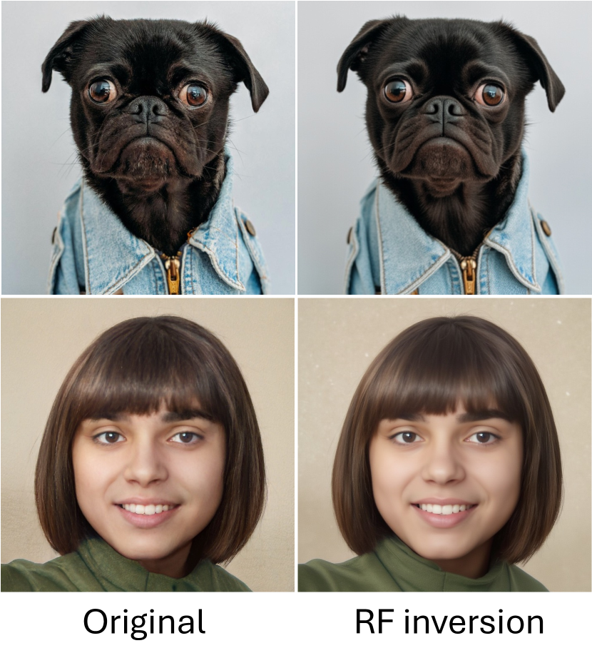
Inversion. The first step involves computing the structured noise ${\mathbf{y}}_{1}$ by employing our controlled ODE (8), initialized at the reference content $Y_{0}={\mathbf{y}}_{0}$. To compute the unconditional vector field, we use the pre-trained Flux model $u\left(\cdot,\cdot,\cdot;\varphi\right)$, which requires three inputs: the state $Y_{t}$, the time $t$, and the prompt embedding $\Phi(\text{prompt})$. During the inversion process, we use null prompt in the Flux model, i.e., $u_{t}({\mathbf{y}}_{t})=u({\mathbf{y}}_{t},t,\Phi(\text{``"});\varphi)$. For the conditional vector field, we apply the analytical solution derived in Proposition 3.2. The inversion process yields a latent variable that is then used to initialize our controlled ODE (15), i.e., $X_{0}={\mathbf{y}}_{1}$. In this phase, we again use the null prompt to compute the vector field $v_{t}({\mathbf{x}}_{t})=-u({\mathbf{x}}_{t},1-t,\Phi(\text{``"});\varphi)$: see Figure 3 for the final output.

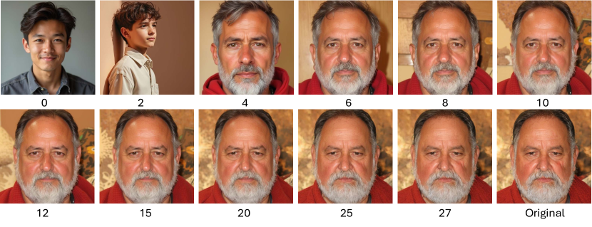
Editing. The second step involves text-guided editing of the reference content ${\mathbf{y}}_{0}$. This process is governed by our controlled ODE (15), where the vector field is computed using the desired text prompt within Flux: $v_{t}(X_{t})=-u({\mathbf{x}}_{t},1-t,\Phi(\text{prompt});\varphi)$. The controller guidance $\eta$ in (15) balances faithfulness and editability: higher $\eta$ improves faithfulness but limits editability, while lower $\eta$ allows significant edits at the cost of reduced faithfulness. Consequently, the controller guidance $\eta$ provides a smooth interpolation between faithfulness and editability, a crucial feature in semantic image editing. Motivated by Remark 3.3 and 3.6, we consider a time-varying controller guidance $\eta_{t}$, such that for a fixed $\eta\in[0,1]$ and $\tau\in[0,1]$, $\eta_{t}=\eta~{}\forall t\leq\tau$ and $0$ otherwise. Figure 4 illustrates the effect of controller guidance $\eta$ for $\tau=0.3$; see Appendix C.2 for a detailed ablation study.

Figure 4: Effect of controller guidance $\eta$ given the original image and the prompt: “A young man”. Increasing $\eta$ improves the faithfulness to the original image, which is reconstructed at $\eta\!=\!1$.

Figure 5: Stroke2Image generation. Our method generates photo-realistic images of bedroom or church given stroke paints, showing robustness to initial corruptions.

Figure 6: Image editing for adding face accessories. Prompt: “face of a man/woman wearing glasses”. The proposed method better preserves the identity while applying the desired edits.

5 Experimental Evaluation

We show that RF inversion outperforms DM inversion across three benchmarks: LSUN-church, LSUN-bedroom (Wang et al., 2017), and SFHQ (Beniaguev, 2022) on two tasks: Stroke2Image generation and semantic image editing. Stroke2Image generation shows the robustness of our algorithm to initial corruption. In semantic image editing, we emphasize the ability to edit clean images without additional training, optimization, or complex attention processors.

Baselines. As this paper focuses on inverting flows, we compare with SoTA inversion approaches, such as NTI (Mokady et al., 2023), DDIM Inversion (Song et al., 2021a), and SDEdit (Meng et al., 2022). We use the official NTI implementation for both NTI and DDIM inversion, and Diffusers library for SDEdit. Hyper-parameters for all these baselines are tuned for optimal performance. We compare with NTI for both direct prompt change and with prompt-to-prompt Hertz et al. (2022) editing. All methods are training-free; however, NTI (Mokady et al., 2023) solves an optimization problem at each denoising step during inversion and uses P2P (Hertz et al., 2022) attention processor during editing. We follow the evaluation protocol from SDEdit (Meng et al., 2022). More qualitative results and comparison are in Appendix §C.

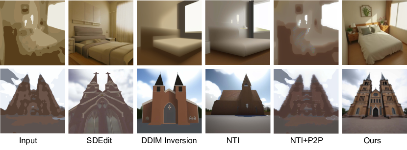
Stroke2Image generation. As discussed in §4, our goal is to generate a photo-realistic image from a stroke paint (a corrupted image) and the text prompt “photo-realistic picture of a bedroom”. In this case, the high level details in the stroke painting guide the reverse process toward a clean image.

In Figure 5, we compare RF inversion (ours) with DM inversions. DM inversions propagate the corruption from the stroke painting into the structured noise, which leads to outputs resembling the input stroke painting. NTI optimizes null embeddings to align the reverse process with the DDIM forward trajectory. Although adding P2P to the NTI pipeline helps localized editing as in Figure 6, for corrupted images, it drives the reverse process even closer to the corruption. In contrast, our controlled ODE (8) yields a structured noise that is consistent with the corrupted image and also the invariant terminal distribution, as discussed in §3.3, resulting in more realistic images.

In Table 1, we show that our method outperforms prior works in faithfulness and realism. On the test split of LSUN bedroom dataset, our approach is 4.7% more faithful and 13.79% more realistic than the best optimization free method SDEdit-SD1.5. Ours is 73% more realistic than the optimization-based method NTI, but comparable in L2. As discussed, NTI+P2P gets closer toward the corrupt image, which gives a very low L2 error, but the resulting image becomes unrealistic. Our approach is 89% more realistic than NTI+P2P. We observe similar gains on LSUN church dataset.

User study. We conduct a user study using Amazon Mechanical Turk to evaluate the overall performance of the our method. With 3 responses for each question, we collected in total 9,000 comparisons from 126 participants. As given in Table 1, our method outperforms all the other baselines by at least 59.67% in terms of overall satisfaction. More details are provided in Appendix §C.6.

Figure 7: Editing (a) stylized expression, (b) age, (c) gender, and (d) object insert. Given an original image and a text prompt, our algorithm performs semantic image editing in the wild.

Table 1: Quantitative results for Stroke2Image generation. L2 and Kernel Inception Distance (KID) capture faithfulness and realism, respectively. Optimization-based methods are colored gray. User Pref. shows the percentage of users that prefer our method over each alternative in pairwise comparisons (and ties). E.g.: 62.11% (+ 8% ties) prefer ours over SDEdit-Flux for LSUN Bedroom.

	LSUN Bedroom			LSUN Church
Method	L2 $\downarrow$	KID $\downarrow$	User Pref. (%) $\uparrow$	L2 $\downarrow$	KID $\downarrow$	User Pref. (%) $\uparrow$
SDEdit-SD1.5	86.72	0.029	59.67 (5.33)	90.72	0.089	65.33 (4.11)
SDEdit-Flux	94.89	0.032	62.11 (8.00)	92.47	0.081	66.22 (5.22)
DDIM Inv.	87.95	0.113	82.56 (1.67)	97.36	0.107	85.44 (2.78)
NTI	82.77	0.095	80.89 (4.33)	87.88	0.098	77.11 (4.89)
NTI+P2P	46.46	0.234	98.11 (1.78)	34.48	0.168	99.22 (0.56)
Ours	82.65	0.025	-	80.36	0.059	-

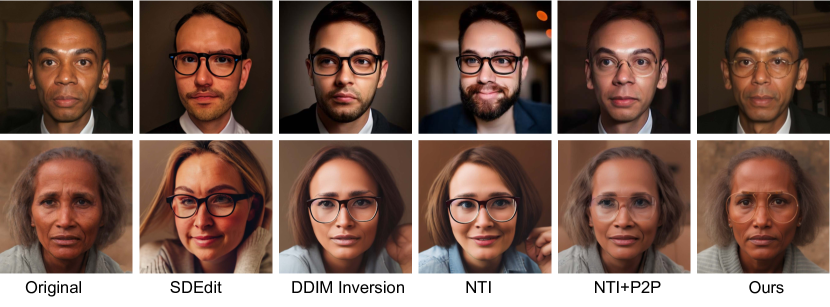
Semantic Image Editing. Given a clean image and a text “prompt”, the objective is to modify the image according to the given text while preserving the contents of the image (identity for face images). In rectified linear paths, editing from a noisy latent becomes straightforward, further enhancing the efficiency of our approach. Compared with SoTA approaches (Figure 6), our method requires no additional optimization or complex attention processors as in NTI (Mokady et al., 2023)+P2P(Hertz et al., 2022). Thus, it is more efficient than a current SoTA approach, and importantly, more faithful to the original image while applying the desired edits.

Figure 8: Comparison using Flux backbone.

In Table 2, we show that our method outperforms the optimization-free methods by at least 29% in face reconstruction, 6.6% in DINO patch-wise similarity, and 26.4% in CLIP-Image similarity while being comparable in prompt alignment metric CLIP-T. Importantly, our approach offers 54.11% gain in runtime, though it uses a larger ($\sim$12X) model, while staying comparable to NTI+P2P.

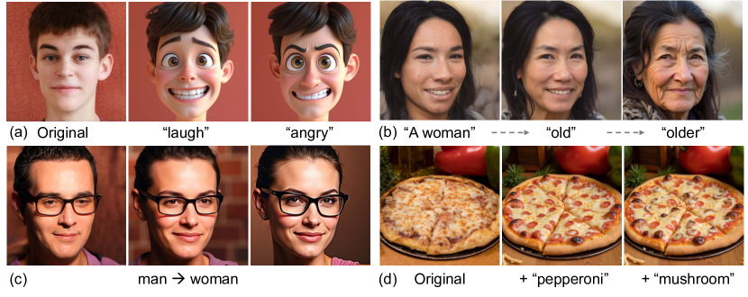
In Figure 7, we showcase four complex editing tasks: (a) prompt-based stylization with the prompt: “face of a boy in disney 3d cartoon style”, where facial expressions, such as “laugh” or “angry” are used for editing; (b) ability to control the age of a person; (c) interpolating between two concepts: “A man” $\leftrightarrow$ “A woman”; (d) sequentially inserting pepperoni and mushroom to an image of a pizza. We provide more examples of editing in the wild in Appendix §C.

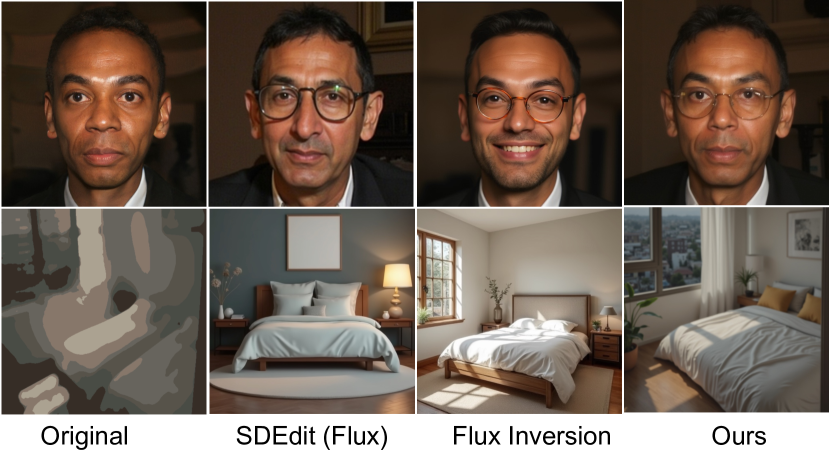
Comparison using the same backbone: Flux. In Figure 8, we compare our method with SDEdit and DDIM inversion both adapted to Flux. NTI optimizes null embeddings to align with forward latents before applying text-guided edits via P2P, an approach well-suited for DMs that use both null and text embedding. However, this strategy cannot be applied to Flux, as it does not explicitly use null embedding. Consequently, we only reimplement SDEdit and DDIM inversion for Flux and compare them to our method. Since all methods leverage the same generative model, the improvements clearly stem from our controlled ODEs, grounded in a solid theoretical foundation (§3).

Table 2: Quantitative results for face editing on SFHQ for “wearing glasses”.

Method	Face Rec. $\downarrow$	DINO $\uparrow$	CLIP-T $\uparrow$	CLIP-I $\uparrow$	Runtime(s) $\downarrow$
SDEdit-SD1.5	0.626	0.885	0.300	0.712	8
SDEdit-Flux	0.632	0.892	0.292	0.710	24
DDIM Inv.	0.709	0.884	0.311	0.669	15
NTI	0.707	0.876	0.304	0.666	78
NTI+P2P	0.443	0.953	0.293	0.845	85
Ours	0.442	0.951	0.300	0.900	39

6 Conclusion

We present the first efficient approach for inversion and editing with the state-of-art rectified flow models such as Flux. Our method interpolates between two vector fields: (i) the unconditional RF field that transforms a “clean” image to “typical” noise, and (ii) a conditional vector field derived from optimal control that transforms any image (clean or not) to “typical” noise. Our new field thus navigates between these two competing objectives of consistency with the given (possibly corrupted) image, and consistency with the distribution of clean images. Theoretically, we show that this is equivalent to a new rectified SDE formulation, sharing this intuition of interpolation. Practically, we show that our method results in state-of-art zero-shot performance, without the need of additional training, optimization of latent variables, prompt tuning, or complex attention processors. We demonstrate the effectiveness of our method in stroke-to-image synthesis, face editing, object insertion, and stylization tasks, with large-scale human evaluation confirming user preference.

Limitation. The lack of comparison with expensive diffusion-based editing solutions may be viewed as a limitation. However, these implementations are either not available for Flux or not directly applicable due to Flux’s distinct multi-modal architecture. The key contribution of this paper lies in its theoretical foundations, validated using standard benchmarks and relevant baselines.

Reproducibility. The pseudocode and hyper-parameter details have been provided to reproduce the reported results in this paper.

Broader Impact Statement

Semantic image inversion and editing have both positive and negative social impacts.

On the positive side, this technology enables (i) the generation of photo-realistic images from high level descriptions, such as stroke paintings, and (ii) the modification of clean images by changing various attributes like the age, gender, or adding glasses (§5).

On the negative side, it can be misused by malicious users to manipulate photographs of individuals with inappropriate or offensive edits. Additionally, it carries the inherent risks associated with the underlying generative model.

To mitigate the negative social impacts, we enable safety features such as NSFW filters in the underlying generative model. Furthermore, we believe watermarking images generated by this technology can reduce misuse, especially in inversion and editing applications.

Appendix A Additional Theoretical Results

In this section, we present the theoretical results omitted from the main draft due to space constraints. We formalize the ODE derivation of the standard rectified flows in Lemma A.1.

Lemma A.1.

Given a coupling $(Y_{0},Y_{1})\sim p_{0}\times p_{1}$, consider the noising process $Y_{t}=tY_{1}+(1-t)Y_{0}$. Then, the rectified flow ODE formulation with the optimal vector field is given by

$$\mathrm{d}Y_{t}=\left[-\frac{1}{1-t}Y_{t}-\frac{t}{1-t}\nabla\log p_{t}(Y_{t})\right]\mathrm{d}t,\quad Y_{0}\sim p_{0}.$$ (19)

Furthermore, denoting $p_{t}(\cdot)$ as the marginal pdf of $Y_{t}$, its density evolution is given by:

$$\frac{\partial p_{t}(Y_{t})}{\partial t}=\nabla\cdot\left[\left(\frac{1}{1-t}Y_{t}+\frac{t}{1-t}~{}\nabla\log p_{t}(Y_{t})\right)p_{t}(Y_{t})\right].$$ (20)

In Lemma A.2, we show that the marginal distribution of the rectified flow (6) is equal to that of an SDE with appropriate drift and diffusion terms.

Lemma A.2.

Fix any $T\in(0,1)$, and for any $t\in[0,T]$, the density evolution (20) of the rectified flow model (19) is identical to the density evolution of the following SDE:

$$\mathrm{d}Y_{t}=-\frac{1}{1-t}Y_{t}\mathrm{d}t+\sqrt{\frac{2t}{1-t}}\mathrm{d}W_{t},\quad Y_{0}\sim p_{0}.$$ (21)

In Proposition A.3, we show that the stationary distribution of the SDE (21) converges to the standard Gaussian ${\mathcal{N}}(0,I)$ in the limit as $t\rightarrow 1$.

Proposition A.3.

Fix any $T\in(0,1)$, and for any $t\in[0,T]$, the density evolution for the rectified flow ODE (6) is same as that of the SDE (12). Furthermore, denoting $p_{t}(\cdot)$ as the marginal pdf of $Y_{t}$, its stationary distribution $p_{t}(Y_{t})\propto\exp{(-\frac{\left\|Y_{t}\right\|^{2}}{2t})}$, which converges to ${\mathcal{N}}\left(0,I\right)$ as $t\rightarrow 1$.

We note that Lemma A.1 and Lemma A.2 follow from the duality between the heat equation and the continuity equation (Øksendal, 2003), where it is classically known that one can interpret a diffusive term as a vector field that is affine in the score function, and vice-versa. This connection has been carefully used to study a large family of stochastic interpolants (that generalize rectified flows) in (Albergo & Vanden-Eijnden, 2023; Albergo et al., 2023), and which can lead to a family of ODE-SDE pairs. In the lemmas above, we have provided explicit coefficients that have been directly derived, instead of using the stochastic interpolant formulation. Our key contribution lies in constructing a controlled ODEs (8) and (15), along with their equivalent SDEs (10) and (17) in Theorem 3.4 and Theorem 3.5, respectively. This aids faithfulness and editability as discussed in §4.

In Lemma A.4, we derive a rectified SDE that transforms noise into images by reversing the stochastic equivalent of rectified flows (12).

Lemma A.4.

Fix any small $\delta\in(0,1)$, and for any $t\in[\delta,1]$, the process $X_{t}$ governed by the SDE:

$$\mathrm{d}X_{t}=\left[\frac{1}{t}X_{t}+\frac{2(1-t)}{t}\nabla\log p_{1-t}(X_{t})\right]\mathrm{d}t+\sqrt{\frac{2(1-t)}{t}}\mathrm{d}W_{t},\quad X_{0}\sim p_{1},$$ (22)

is the time-reversal of the SDE (12).

Implication. The reverse SDE (22) provides a stochastic sampler for SoTA rectified flow models like Flux. Unlike diffusion-based generative models that explicitly model the score function $\nabla\log p_{t}(\cdot)$ in (22), rectified flows model a vector field, as discussed in §3.1. However, given a neural network $u({\mathbf{y}}_{t},t;\varphi))$ approximating the vector field $u_{t}({\mathbf{y}}_{t})$, Lemma A.1 offers an explicit formula for computing the score function:

$$\nabla\log p_{t}(Y_{t})=-\frac{1}{t}Y_{t}-\frac{1-t}{t}u(Y_{t},t;\varphi).$$ (23)

This score function is used to compute the drift and diffusion coefficients of the SDE (22), resulting in a practically implementable stochastic sampler for Flux. This extends the applicability of Flux to downstream tasks where SDE-based samplers have demonstrated practical benefits, as seen in diffusion models (Ho et al., 2020; Song et al., 2021b; Rombach et al., 2022; Podell et al., 2023).

Appendix B Technical Proofs

This section contains technical proofs of the theoretical results presented in this paper.

B.1 Proof of Proposition 3.2

Proof.

The standard approach to solving an LQR problem is the minimum principle theorem that can be found in control literature (Fleming & Rishel, 1975; Basar et al., 2020). We follow this approach and provide the full proof below for completeness.

The Hamiltonian of the LQR problem (7) is given by

$$H({\mathbf{z}}_{t},{\mathbf{p}}_{t},{\mathbf{c}}_{t},t)=\frac{1}{2}\left\|{\mathbf{c}}_{t}\right\|^{2}+{\mathbf{p}}_{t}^{T}{\mathbf{c}}_{t}.$$ (24)

For ${\mathbf{c}}_{t}^{*}=-{\mathbf{p}}_{t}$, the Hamiltonian attains its minumum value: $H({\mathbf{z}}_{t},{\mathbf{p}}_{t},{\mathbf{c}}_{t}^{*},t)=-\frac{1}{2}\left\|{\mathbf{p}}_{t}\right\|^{2}$. Using minimum principle theorem (Fleming & Rishel, 1975; Basar et al., 2020), we get

$$\frac{\mathrm{d}{\mathbf{p}}_{t}}{\mathrm{d}t} =\nabla_{{\mathbf{z}}_{t}}H\left({\mathbf{z}}_{t},{\mathbf{p}}_{t},{\mathbf{c}}_{t}^{*},t\right)=0;$$ (25)

$$\frac{\mathrm{d}{\mathbf{z}}_{t}}{\mathrm{d}t} =\nabla_{{\mathbf{p}}_{t}}H\left({\mathbf{z}}_{t},{\mathbf{p}}_{t},{\mathbf{c}}_{t}^{*},t\right)=-{\mathbf{p}}_{t};$$ (26)

$${\mathbf{z}}_{0} ={\mathbf{y}}_{0};$$ (27)

$${\mathbf{p}}_{1} =\nabla_{{\mathbf{z}}_{1}}\left(\frac{\lambda}{2}\left\|{\mathbf{z}}_{1}-{\mathbf{y}}_{1}\right\|_{2}^{2}\right)=\lambda\left({\mathbf{z}}_{1}-{\mathbf{y}}_{1}\right).$$ (28)

From (25), we know ${\mathbf{p}}_{t}$ is a constant ${\mathbf{p}}$. Using this constant in (26) and integrating from $t\rightarrow 1$, we have ${\mathbf{z}}_{1}={\mathbf{z}}_{t}-{\mathbf{p}}(1-t)$. Substituting ${\mathbf{z}}_{1}$ in (27),

$${\mathbf{p}}=\lambda({\mathbf{z}}_{t}-{\mathbf{p}}(1-t)-{\mathbf{y}}_{1})=\lambda({\mathbf{z}}_{t}-{\mathbf{y}}_{1})-\lambda(1-t){\mathbf{p}},$$

which simplifies to

$${\mathbf{p}}=\left(1+\lambda(1-t)\right)^{-1}\lambda({\mathbf{z}}_{t}-{\mathbf{y}}_{1})=\left(\frac{1}{\lambda}+(1-t)\right)^{-1}({\mathbf{z}}_{t}-{\mathbf{y}}_{1}).$$

Taking the limit $\lambda\rightarrow\infty$, we get ${\mathbf{p}}=\frac{{\mathbf{z}}_{t}-{\mathbf{y}}_{1}}{1-t}$ and the optimal controller ${\mathbf{c}}_{t}^{*}=\frac{{\mathbf{y}}_{1}-{\mathbf{z}}_{t}}{1-t}$. Since $u_{t}({\mathbf{z}}_{t}|{\mathbf{y}}_{1})={\mathbf{y}}_{1}-{\mathbf{y}}_{0}$, the proof follows by substituting ${\mathbf{y}}_{0}=\frac{{\mathbf{z}}_{t}-t{\mathbf{y}}_{1}}{1-t}$. ∎

B.2 Proof of Proposition 3.1

Proof.

Initializing the generative ODE (1) with the structured noise ${\mathbf{y}}_{1}$, we get

$$\frac{\mathrm{d}X_{t}}{\mathrm{d}t}=v_{t}(X_{t}),\quad X_{0}={\mathbf{y}}_{1},\quad\forall t\in[0,1].$$ (29)

Substituting $u_{t}(\cdot)=-v_{1-t}(\cdot)$ in ODE (6),

$$\frac{\mathrm{d}Y_{t}}{\mathrm{d}t}=u_{t}(Y_{t})=-v_{1-t}(Y_{t}),\quad Y_{0}={\mathbf{y}}_{0},\quad\forall t\in[0,1].$$

Replacing $t\rightarrow(1-t)$,

$$\frac{\mathrm{d}Y_{1-t}}{\mathrm{d}t}=v_{t}(Y_{1-t}),\quad\forall t\in[0,1].$$ (30)

Since (29) and (30) hold $\forall t\in[0,1]$ and $X_{0}={\mathbf{y}}_{1}$, then $X_{t}=Y_{1-t}$ that implies $X_{1}=Y_{0}={\mathbf{y}}_{0}$. ∎

B.3 Proof of Theorem 3.4

Proof.

From Proposition 3.2, we have $u_{t}(Y_{t}|Y_{1})=\frac{Y_{1}-Y_{t}}{1-t}$. In Lemma A.1, we show that

$$u_{t}(Y_{t})=\left[-\frac{1}{1-t}Y_{t}-\frac{t}{1-t}\nabla\log p_{t}(Y_{t})\right].$$

Now, the controlled ODE (8) becomes:

$$\mathrm{d}Y_{t} =\Big{[}u_{t}(Y_{t})+\gamma\left(u_{t}(Y_{t}|Y_{1})-u_{t}(Y_{t})\right)\Big{]}\mathrm{d}t,\quad Y_{0}\sim p_{0},\quad Y_{1}={\mathbf{y}}_{1}$$

$$=\left[(1-\gamma)\left(-\frac{1}{1-t}Y_{t}-\frac{t}{1-t}\nabla\log p_{t}(Y_{t})\right)+\gamma\left(\frac{Y_{1}-Y_{t}}{1-t}\right)\right]\mathrm{d}t$$

$$=\left[-\frac{1}{1-t}Y_{t}-\frac{t}{1-t}(1-\gamma)\nabla\log p_{t}(Y_{t})+\frac{\gamma}{1-t}Y_{1}\right]\mathrm{d}t$$

$$=\left[-\frac{1}{1-t}\left(Y_{t}-\gamma Y_{1}\right)-\frac{t}{1-t}(1-\gamma)\nabla\log p_{t}(Y_{t})\right]\mathrm{d}t.$$

Using continuity equation (Øksendal, 2003), the density evolution of the controlled ODE (8) then becomes:

$$\frac{\partial p_{t}(Y_{t})}{\partial t}=\nabla\cdot\left[\left(\frac{1}{1-t}\left(Y_{t}-\gamma Y_{1}\right)+\frac{t}{1-t}(1-\gamma)\nabla\log p_{t}(Y_{t})\right)p_{t}(Y_{t})\right].$$ (31)

Applying Fokker-Planck equation (Øksendal, 2003) to the SDE (10), we have

$$\frac{\partial p_{t}(Y_{t})}{\partial t}+\nabla\cdot\left[\left(-\frac{1}{1-t}\left(Y_{t}-\gamma Y_{1}\right)\right)p_{t}(Y_{t})\right]=\nabla\cdot\left[\frac{t}{1-t}(1-\gamma)\nabla p_{t}(Y_{t})\right],$$

which can be rearranged to equal (31) completing the proof. ∎

B.4 Proof of Lemma A.1

Proof.

Given $(Y_{0},Y_{1})\sim p_{0}\times p_{1}$, the conditional flow matching loss (5) can be reparameterized as:

$${\mathcal{L}}_{CFM}(\varphi)\coloneqq\mathbb{E}_{t\sim{\mathcal{U}}[0,1],(Y_{0},Y_{1})\sim p_{1}\times p_{0}}\left[\left\|(Y_{1}-Y_{0})-u(Y_{t},t;\varphi)\right\|_{2}^{2}\right],\quad Y_{t}=tY_{1}+(1-t)Y_{0},$$

where the optimal solution is given by the minimum mean squared estimator:

$$u_{t}({\mathbf{y}}_{t})=\mathbb{E}_{(Y_{0},Y_{1})\sim p_{1}\times p_{0}}\left[Y_{1}-Y_{0}|Y_{t}={\mathbf{y}}_{t}\right].$$ (32)

Since $Y_{t}=tY_{1}+(1-t)Y_{0}$, we use Tweedie’s formula (Efron, 2011) to compute

$$\mathbb{E}\left[Y_{0}|Y_{t}={\mathbf{y}}_{t}\right]=\frac{1}{1-t}{\mathbf{y}}_{t}+\frac{t^{2}}{1-t}\nabla\log p_{t}({\mathbf{y}}_{t}).$$ (33)

Using the above relation, we obtain the following:

$$\mathbb{E}\left[Y_{1}|Y_{t}={\mathbf{y}}_{t}\right] =\frac{1}{t}\mathbb{E}\left[Y_{t}-(1-t)Y_{0}|Y_{t}={\mathbf{y}}_{t}\right]$$

$$=\frac{1}{t}\left({\mathbf{y}}_{t}-(1-t)\mathbb{E}\left[Y_{0}|Y_{t}={\mathbf{y}}_{t}\right]\right)$$

$$=\frac{1}{t}\left({\mathbf{y}}_{t}-(1-t)\left(\frac{1}{1-t}{\mathbf{y}}_{t}+\frac{t^{2}}{1-t}\nabla\log p_{t}({\mathbf{y}}_{t})\right)\right)$$

$$=-t~{}\nabla\log p_{t}({\mathbf{y}}_{t}).$$ (34)

Combining (33) and (34) using linearity of expectation, we get

$$u_{t}({\mathbf{y}}_{t}) =\mathbb{E}\left[Y_{1}|Y_{t}={\mathbf{y}}_{t}\right]-\mathbb{E}\left[Y_{0}|Y_{t}={\mathbf{y}}_{t}\right]$$ (35)

$$=-t~{}\nabla\log p_{t}({\mathbf{y}}_{t})-\frac{1}{1-t}{\mathbf{y}}_{t}-\frac{t^{2}}{1-t}\nabla\log p_{t}({\mathbf{y}}_{t})$$ (36)

$$=-\frac{1}{1-t}{\mathbf{y}}_{t}-\frac{t}{1-t}\nabla\log p_{t}({\mathbf{y}}_{t}),$$ (37)

The density evolution of $Y_{t}$ now immediately follows from the continuity equation (Øksendal, 2003) applied to (19). ∎

B.5 Proof of Lemma A.2

Proof.

The Fokker-Planck equation of the SDE (12) is given by

$$\frac{\partial p_{t}(Y_{t})}{\partial t}+\nabla\cdot\left[-\frac{1}{1-t}Y_{t}~{}p_{t}(Y_{t})\right]=\nabla\cdot\left[\frac{t}{1-t}~{}\nabla p_{t}(Y_{t})\right].$$ (38)

Rearranging (38) by multiplying and dividing $p_{t}(Y_{t})$ in the right hand side, we get

$$\frac{\partial p_{t}(Y_{t})}{\partial t}=\nabla\cdot\left[\left(\frac{1}{1-t}Y_{t}+\frac{t}{1-t}~{}\nabla\log p_{t}(Y_{t})\right)p_{t}(Y_{t})\right].$$ (39)

To conclude, observe that that the density evolution above is identical to (20). ∎

B.6 Proof of Proposition A.3

Proof.

The optimal vector field of the rectified flow ODE (6) is given by Lemma A.1. The proof then immediately follows from the Fokker-Planck equations in Lemma A.1 and Lemma A.2.

From Lemma A.2, the density evolution of the SDE (12) is given by

$$\frac{\partial p_{t}(Y_{t})}{\partial t}=\nabla\cdot\left[\left(\frac{1}{1-t}Y_{t}+\frac{t}{1-t}~{}\nabla\log p_{t}(Y_{t})\right)p_{t}(Y_{t})\right].$$

The stationary (or steady state) distribution satisfies the following:

$$\frac{\partial p_{t}(Y_{t})}{\partial t}=0=\nabla\cdot\left[\left(\frac{1}{1-t}Y_{t}+\frac{t}{1-t}~{}\nabla\log p_{t}(Y_{t})\right)p_{t}(Y_{t})\right].$$

Using the boundary conditions (Øksendal, 2003), we get

$$\frac{1}{1-t}Y_{t}+\frac{t}{1-t}~{}\nabla\log p_{t}(Y_{t})=0,$$

which immediately implies $p_{t}(Y_{t})\propto e^{-\frac{\left\|Y_{t}\right\|^{2}}{2t}}$. ∎

B.7 Proof of Theorem 3.5

Proof.

Using Fokker-Planck equation (Øksendal, 2003), Lemma A.4 implies

$$\frac{\partial q_{t}(X_{t})}{\partial t}=\nabla\cdot\left[-q_{t}(X_{t})\left(\frac{1}{t}X_{t}+\frac{1-t}{t}\nabla\log q_{t}(X_{t})\right)\right].$$

Therefore, the optimal vector field $v_{t}(X_{t})$ of the controlled ODE (15) is given by

$$v_{t}(X_{t})=\frac{1}{t}X_{t}+\frac{1-t}{t}\nabla\log p_{1-t}(X_{t}).$$ (40)

The LQR problem (16) is identical to the LQR problem (7) with changes in the initial and terminal states. Similar to Proposition 3.2, we compute the closed-form solution for the conditional vector field of the ODE (15) as:

$$v_{t}(X_{t}|X_{1})=\frac{X_{1}-X_{t}}{1-t}.$$ (41)

Combining (40) and (41), we have

$$\mathrm{d}X_{t} =\left[v_{t}(X_{t})+\eta(v_{t}(X_{t}|X_{1})-v_{t}(X_{t}))\right]\mathrm{d}t$$

$$=\left[(1-\eta)\left(\frac{1}{t}X_{t}+\frac{1-t}{t}\nabla\log p_{1-t}(X_{t})\right)+\eta\left(\frac{X_{1}-X_{t}}{1-t}\right)\right]\mathrm{d}t$$

$$=\left[\frac{(1-\eta)(1-t)-\eta t}{t(1-t)}X_{t}+\frac{\eta}{1-t}X_{1}+\frac{(1-\eta)(1-t)}{t}\nabla\log p_{1-t}(X_{t})\right]\mathrm{d}t$$

$$=\left[\frac{1-t-\eta}{t(1-t)}X_{t}+\frac{\eta}{1-t}X_{1}+\frac{(1-\eta)(1-t)}{t}\nabla\log p_{1-t}(X_{t})\right]\mathrm{d}t.$$

The resulting continuity equation (Øksendal, 2003) becomes:

$$\frac{\partial q_{t}(X_{t})}{\partial t} =\nabla\cdot\left[-\left(\frac{1-t-\eta}{t(1-t)}X_{t}+\frac{\eta}{1-t}X_{1}+\frac{(1-\eta)(1-t)}{t}\nabla\log p_{1-t}(X_{t})\right)q_{t}(X_{t})\right]$$

$$=\nabla\cdot\Bigg{[}-\left(\frac{1-t-\eta}{t(1-t)}X_{t}+\frac{\eta}{1-t}X_{1}+\frac{2(1-\eta)(1-t)}{t}\nabla\log p_{1-t}(X_{t})\right)q_{t}(X_{t})$$

$$\hskip 142.26378pt+\left(\frac{(1-\eta)(1-t)}{t}\nabla\log p_{1-t}(X_{t})\right)q_{t}(X_{t})\Bigg{]}.$$

Using time-reversal property from Propsition 3.2, the above expression simplifies to

$$\frac{\partial q_{t}(X_{t})}{\partial t} +\nabla\cdot\Bigg{[}\left(\frac{1-t-\eta}{t(1-t)}X_{t}+\frac{\eta}{1-t}X_{1}+\frac{2(1-\eta)(1-t)}{t}\nabla\log p_{1-t}(X_{t})\right)q_{t}(X_{t})\Bigg{]}$$

$$=\nabla\cdot\Bigg{[}\frac{(1-\eta)(1-t)}{t}\nabla q_{t}(X_{t})\Bigg{]},$$

which yields the following SDE:

$$\mathrm{d}X_{t}=\left[\frac{1-t-\eta}{t(1-t)}X_{t}+\frac{\eta}{1-t}X_{1}+\frac{2(1-\eta)(1-t)}{t}\nabla\log p_{1-t}(X_{t})\right]\mathrm{d}t+\sqrt{\frac{2(1-\eta)(1-t)}{t}}\mathrm{d}W_{t},$$

and thus, completes the proof. ∎

B.8 Proof of Lemma A.4

Proof.

It suffices to show that the Fokker-Planck equations of the SDE (22) and (12) are the same after time-reversal. Let $q_{t}(\cdot)$ denote the marginal pdf of $X_{t}$ such that $q_{0}(\cdot)=p_{1}(\cdot)$. The Fokker-Planck equations of the SDE (22) becomes

$$\frac{\partial q_{t}(X_{t})}{\partial t}+\nabla\cdot\left[q_{t}(X_{t})\left(\frac{1}{t}X_{t}+\frac{2(1-t)}{t}\nabla\log p_{1-t}(X_{t})\right)\right]=\nabla\cdot\left[\left(\frac{1-t}{t}\right)\nabla q_{t}(X_{t})\right],$$

which can be rearranged to give

$$\frac{\partial q_{t}(X_{t})}{\partial t} =\nabla\cdot\left[-q_{t}(X_{t})\left(\frac{1}{t}X_{t}+\frac{2(1-t)}{t}\nabla\log p_{1-t}(X_{t})\right)+\left(\frac{1-t}{t}\right)\nabla q_{t}(X_{t})\right]$$

$$=\nabla\cdot\left[-q_{t}(X_{t})\left(\frac{1}{t}X_{t}+\frac{2(1-t)}{t}\nabla\log p_{1-t}(X_{t})-\frac{1-t}{t}\nabla\log q_{t}(X_{t})\right)\right]$$

Since $Y_{t}$ is the time-reversal process of $X_{t}$ as discussed in Proposition (3.1),

$$\frac{\partial q_{t}(X_{t})}{\partial t}=\nabla\cdot\left[-q_{t}(X_{t})\left(\frac{1}{t}X_{t}+\frac{1-t}{t}\nabla\log q_{t}(X_{t})\right)\right].$$

Substituting $t\rightarrow 1-t$,

$$\frac{\partial q_{1-t}(X_{1-t})}{\partial t}=\nabla\cdot\left[q_{1-t}(X_{1-t})\left(\frac{1}{1-t}X_{1-t}+\frac{t}{1-t}\nabla\log q_{1-t}(X_{1-t})\right)\right],$$

which implies the density evolution of (12):

$$\frac{\partial p_{t}(Y_{t})}{\partial t} =\nabla\cdot\left[p_{t}(Y_{t})\left(\frac{1}{1-t}Y_{t}+\frac{t}{1-t}\nabla\log p_{t}(Y_{t})\right)\right].$$

This completes the proof of the statement. ∎

Appendix C Additional Experiments

This section substantiates our contributions further by providing additional experimental details.

Baselines. We use the official NTI codebase for the implementations of NTI (Mokady et al., 2023), P2P (Hertz et al., 2022), and DDIM (Song et al., 2021a) inversion. We use the official Diffusers implementation for SDEdit and Flux. We modify the pipelines for SDEdit and DDIM inversion to adapt to the Flux backbone.

For completeness, we include qualitative comparison with a leading training-based approach InstructPix2Pix (Brooks et al., 2023) and a higher-order differential equation based LEDIT++ (Brack et al., 2024) (§C). Table 3 summarizes the requirements of the compared baselines.

Table 3: Requirements of compared baselines. Our method outperforms prior works while requiring no additional training, optimization of prompt embedding, or attention manipulation scheme.

Method	Training	Optimization	Attention Manipulation
SDEdit (Meng et al., 2022)
DDIM (Song et al., 2021a)
NTI (Mokady et al., 2023)
NTI+P2P (Hertz et al., 2022)
LEDIT++ (Brack et al., 2024)
InstructPix2Pix (Brooks et al., 2023)
Ours

Metrics. Following SDEdit (Meng et al., 2022), we measure faithfulness using L2 loss between the stroke input and the output image, and assess realism using Kernel Inception Distance (KID) between real and generated images. Stroke inputs are generated from RGB images using the algorithm provided in SDEdit. Given the subjective nature of image editing, we conduct a large-scale user study to calculate the user preference metric.

For face editing, we evaluate identity preservation, prompt alignment, and overall image quality using a face recognition metric (Ruiz et al., 2024), CLIP-T scores (Radford et al., 2021), and using CLIP-I scores (Radford et al., 2021), respectively. For the face recognition score, we calculate the L2 distance between the face embedding of the original image and the edited image, obtained from Inception ResNet trained on CASIA-Webface dataset. Similar to SDEdit (Meng et al., 2022), we conduct extensive experiments on Stroke2Image generation, and showcase additional capabilities qualitatively on a wide variety of semantic image editing tasks.

Algorithm. The pseudo-code for getting the structured noise is provided in Algorithm 1, and transforming that noise back to an image is given in Algorithm 2.

Input: Discretization steps $N$, reference image ${\mathbf{y}}_{0}$, prompt embedding network $\Phi$, Flux model $u(\cdot,\cdot,\cdot;\varphi)$, Flux noise scheduler $\sigma:[0,1]\rightarrow\mathbb{R}$

Tunable parameter: Controller guidance $\gamma$

Output: Structured noise $Y_{1}$

1 Initialize $Y_{0}={\mathbf{y}}_{0}$

2 Fix a noise sample ${\mathbf{y}}_{1}$

3 for $i=0$ to $N-1$ do

4       Current time step: $t_{i}=\frac{i}{N}$

5       Next time step: $t_{i+1}=\frac{i+1}{N}$

6       Unconditional vector field: $u_{t_{i}}\left(Y_{t_{i}}\right)=u(Y_{t_{i}},t_{i},\Phi(\text{``"});\varphi)$ $\triangleright$ Proposition 3.1

7       Conditional vector field: $u_{t_{i}}\left(Y_{t_{i}}|{\mathbf{y}}_{1}\right)=\frac{{\mathbf{y}}_{1}-Y_{t_{i}}}{1-t_{i}}$ $\triangleright$ Proposition 3.2

8       Controlled vector field: $\hat{u}_{t_{i}}(Y_{t_{i}})=u_{t_{i}}\left(Y_{t_{i}}\right)+\gamma\left(u_{t_{i}}\left(Y_{t_{i}}|{\mathbf{y}}_{1}\right)-u_{t_{i}}\left(Y_{t_{i}}\right)\right)$ $\triangleright$ODE (8)

9       Next state: $Y_{t_{i+1}}=Y_{t_{i}}+\hat{u}_{t_{i}}(Y_{t_{i}})\left(\sigma(t_{i+1})-\sigma(t_{i})\right)$

10 end for

return $Y_{1}$

Algorithm 1 Controlled Forward ODE (8)

Input: Discretization steps $N$, reference text “prompt”, reference image ${\mathbf{y}}_{0}$, prompt embedding network $\Phi$, Flux model $u(\cdot,\cdot,\cdot;\varphi)$, Flux noise scheduler $\sigma:[0,1]\rightarrow\mathbb{R}$,

          structured noise ${\mathbf{y}}_{1}$

Tunable parameter: Controller guidance $\eta$

Output: Edited image $X_{1}$

1 Initialize $X_{0}={\mathbf{y}}_{1}$

2 for $i=0$ to $N-1$ do

3       Current time step: $t_{i}=\frac{i}{N}$

4       Next time step: $t_{i+1}=\frac{i+1}{N}$

5       Unconditional vector field: $v_{t_{i}}\left(X_{t_{i}}\right)=-u(X_{t_{i}},1-t_{i},\Phi(\text{prompt});\varphi)$ $\triangleright$ Proposition 3.1

6       Conditional vector field: $v_{t_{i}}\left(X_{t_{i}}|{\mathbf{y}}_{0}\right)=\frac{{\mathbf{y}}_{0}-X_{t_{i}}}{1-t_{i}}$ $\triangleright$ Proposition 3.2

7       Controlled vector field: $\hat{v}_{t_{i}}(X_{t_{i}})=v_{t_{i}}\left(X_{t_{i}}\right)+\eta\left(v_{t_{i}}\left(X_{t_{i}}|{\mathbf{y}}_{0}\right)-v_{t_{i}}\left(X_{t_{i}}\right)\right)$ $\triangleright$ODE (15)

8       Next state: $X_{t_{i+1}}=X_{t_{i}}+\hat{v}_{t_{i}}(X_{t_{i}})\left(\sigma(t_{i+1})-\sigma(t_{i})\right)$

9 end for

return $X_{1}$

Algorithm 2 Controlled Reverse ODE (15)

C.1 Hyper-parameter configurations

In Table 4, we provide the hyper-parameters for the empirical results reported in §5. We use a fix $\gamma=0.5$ in our controlled forward ODE (8) and a time-varying guidance parameter $\eta_{t}$ in our controlled reverse ODE (15), as motivated in Remark 3.3 and Remark 3.6. Thus, our algorithm introduces one additional hyper-parameter $\eta_{t}$ into the Flux pipeline. For each experiment, we use a fixed time-varying schedule of $\eta_{t}$ described by starting time ($s$), stopping time $\tau$, and strength ($\eta$). We use the default config for Flux model: 3.5 for classifier-free guidance and 28 for the total number of inference steps.

Table 4: Hyper-parameter configuration of our method for inversion and editing tasks.

Task	Starting Time ($s$)	Controller Guidance ($\eta_{t}$)
		Stopping Time ($\tau$)	Strength ($\eta$)
Stroke2Image	3	5	0.9
Object insert	0	6	1.0
Gender editing	0	8	1.0
Age editing	0	5	1.0
Adding glasses	6	25	0.7
Stylization	0	6	0.9

C.2 Ablation Study

In this section, we conduct ablation study for our controller guidance parameter $\eta_{t}$. We consider two different time-varying schedules for $\eta_{t}$, and show that our controller strength allows for a smooth interpolation between unconditional and conditional generation.

In Figure 9, we show the effect of starting time in controlling the faithfulness of inversion; starting time $s\in[0,1]$ is defined as the time at which our controlled reverse ODE (15) is initialized. The initial state $X_{s}={\mathbf{y}}_{1-s}$ is obtained by integrating the controlled forward ODE (8) from $0\rightarrow 1-s$.

Figure 9: Effect of starting time. Prompt: “A young man”. The number below each figure denotes the starting time scaled by 28 (the total number of denoising steps) for better interpretation. In the absence of controller guidance ($\eta_{t}=0$), increasing the starting time ($s$) in our controlled ODE (15) improves faithfulness to the original image.

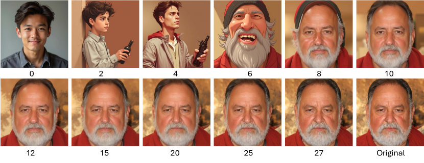
In Figure 10, we study the effect of stopping time. We find that increasing controller guidance $\eta_{t}$ by increasing the stopping time $\tau$ guides the reverse flow towards the original image. However, we observe a phase transition around $\tau=0.14=4/28$, indicating that the resulting drift in our controlled reverse ODE (15) is dominated by the conditional vector field $v_{t}(X_{t}|{\mathbf{y}}_{0})$ for $t\geq\tau$. Therefore, the reverse flow solves the LQR problem (16) and drives toward the terminal state (i.e., the original image).

Figure 10: Effect of controller guidance. Prompt: “A young man”. For a fixed starting time $s=0$, consider a time-varying controller guidance schedule $\eta_{t}=\eta~{}\forall t\leq\tau$ and $0$ otherwise. The number below each figure denotes the stopping time $\tau$ scaled by 28 (the total number of denoising steps) for better interpretation. Increasing $\tau$ increases the controller guidance ($\eta_{t}$) that improves faithfulness to the original image.

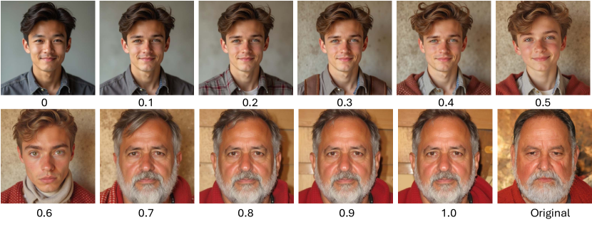
In Figure 11, we visualize the effect of our controller guidance for another time-varying schedule. We make a similar observation as in Figure 10: increasing $\eta_{t}$ improves faithfulness. However, we notice a smooth transition from the unconditional to the conditional vector field, evidence from the smooth interpolation between “A young man” at the top left ($\eta=0$) and the original image at the bottom right.

Figure 11: Effect of controller guidance for another time-varying schedule. Prompt: “A young man”. The number below each figure denotes the starting time scaled by 28 (the total number of denoising steps) for better interpretation. For a fixed starting time $s=0$ and stopping time $\tau=8$, consider a time-varying controller guidance schedule $\eta_{t}=\eta~{}\forall t\leq\tau$ and $0$ otherwise. Increasing $\eta$ increases the controller guidance ($\eta_{t}$) that improves faithfulness to the original image.

C.3 Numerical Simulation

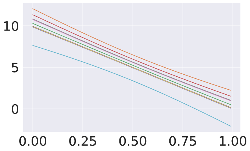
In this section, we design synthetic experiments to compare reconstruction accuracy of DM and RF inversion. Given $Y_{0}\sim p_{0}$, where the data distribution $p_{0}\coloneqq{\mathcal{N}}(\mu,I)$ and the source distribution $q_{0}\coloneqq{\mathcal{N}}(0,I)$, we numerically simulate the ODEs and SDEs associated with DM and RF inversion; see our discussion in §3.

For $\mu=10$, we fix $\gamma=0.5$ in the controlled forward ODE (8), and $\eta=0.5$ in the controlled reverse ODE (15). These ODEs are simulated using the Euler discretization scheme with 100 steps. Additionally, we simulate the uncontrolled rectified flow ODEs (6) $\rightarrow$ (1) as a special case of our controlled ODEs (8) $\rightarrow$ (15) by setting $\gamma=\eta=0$, and the deterministic diffusion model DDIM (Song et al., 2021a) in the same experimental setup.

The inversion accuracy is reported in Table 5. Observe that RF inversion has less L2 and L1 error compared to DDIM inversion (14). The minimum error is obtained by setting $\gamma=\eta=0$ (i.e., reversing the standard rectified flows), which supports our discussion in §3.3.

Furthermore, we simulate the stochastic samplers corresponding to these ODEs in Table 5, highlighted in orange. Similar to the deterministic samplers, we observe that stochastic equivalents of rectified flows more accurately recover the original sample compared to diffusion models. Our controller in RF Inversion (10) $\rightarrow$ (17) effectively reduces the reconstruction error in the uncontrolled RF Inversion (12) $\rightarrow$ (22), which are special cases when $\gamma=\eta=0$. Thus, we demonstrate that (controlled) rectified stochastic processes are better at inverting a given sample from the target distribution, outperforming the typical OU process used in diffusion models (Song & Ermon, 2019; Ho et al., 2020; Song et al., 2021a; b).

Table 5: DM and RF inversion accuracy. Stochastic samplers are highlighted in orange.

Method	L2 Error	L1 Error
DDIM Inversion (14)	6.024	19.038
DDPM Inversion (13)	6.007	15.758
RF Inversion ($\gamma=\eta=0$) (8) $\rightarrow$ (15)	0.092	0.20
RF Inversion ($\gamma=\eta=0$) (10) $\rightarrow$ (17)	3.564	8.795
RF Inversion ($\gamma=0.5,\eta=0$) (8) $\rightarrow$ (15)	4.777	11.628
RF Inversion ($\gamma=0,\eta=0.5$) (8) $\rightarrow$ (15)	1.219	3.074
RF Inversion ($\gamma=0.5,\eta=0.5$) (8) $\rightarrow$ (15)	0.628	1.643
RF Inversion ($\gamma=\eta=0.5$) (10) $\rightarrow$ (17)	0.269	0.694
RF Inversion ($\gamma=\eta=1.0$) (10) $\rightarrow$ (17)	0.003	0.010

In Figure 12, we compare sample paths of diffusion models and recitified flows using 10 IID samples drawn from $p_{0}$. In Figure 13, we visualize paths for those samples using our controlled ODEs and SDEs with $\gamma=\eta=0.5$.

(a) DDPM (13) Fwd.

(b) DDIM (14) Fwd.

(c) SDE (12) Fwd.

(d) RF (6) Fwd.

(e) DDPM (13) Rev.

(f) DDIM (14) Rev.

(g) SDE (12) Rev.

(h) RF (6) Rev.

Figure 12: Sample paths of DMs and RFs. Top row corresponds to the forward process $\{Y_{t}\}$, and bottom row, reverse process $\{X_{t}\}$. In each plot, time is along the horizontal axis and the process, along the vertical axis. The sample paths of RFs are straighter than that of DMs, allowing coarse discretization and faithful reconstruction.

(a) ODE (8) Fwd.

(b) ODE (15) Rev.

(c) SDE (10) Fwd.

(d) SDE (17) Rev.

Figure 13: Sample paths of our controlled ODEs and SDEs. (a,c) The optimal controller $u_{t}(Y_{t}|Y_{1})$ steers $Y_{t}$ towards the terminal state $Y_{1}\sim p_{1}$ during inversion. (b,d) Similarly, $v_{t}(X_{t}|Y_{0})$ guides $X_{t}$ towards the reference image $Y_{0}\sim p_{0}$, significantly reducing the reconstruction error.

C.4 Additional Results on Stroke2Image Generation

In Figure 14 and Figure 15, we show additional qualitative results on Stroke2Image generation. Our method generates more realistic images compared to leading training-free approaches in semantic image editing including optimization-based NTI (Mokady et al., 2023) and attention-based NTI+P2P (Hertz et al., 2022). Furthermore, it gives a competitive advantage over the training-based approach InstructPix2Pix (Brooks et al., 2023).

Figure 14: Stroke2Image generation. Additional qualitative results on LSUN-Bedroom dataset comparing our method with SoTA training-free and training-based editing approaches.

Figure 15: Stroke2Image generation. Additional qualitative results on LSUN-Church dataset comparing our method with SoTA training-free and training-based editing approaches.

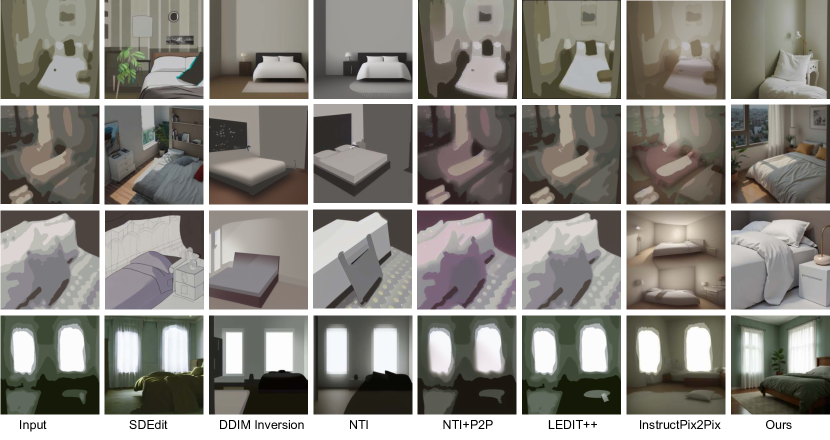
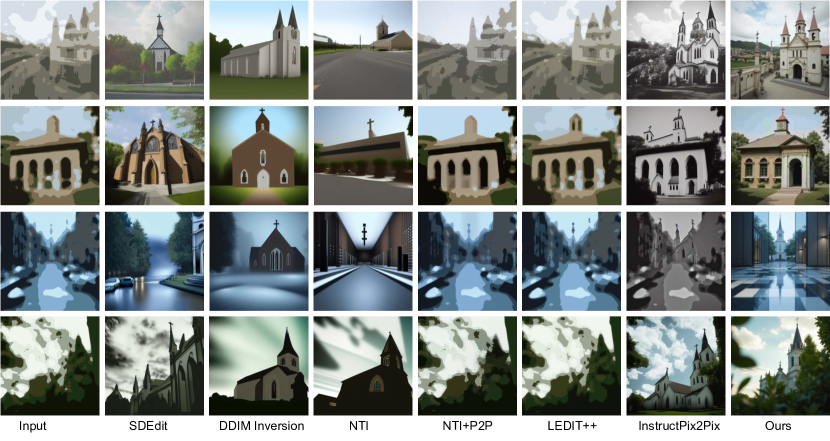
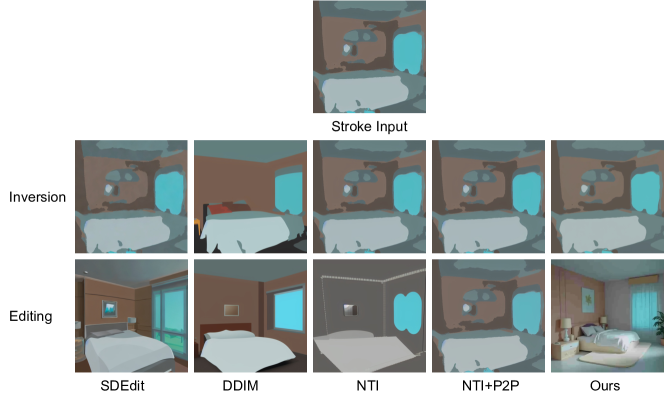
In Figure 16, we demonstrate the robustness of our approach to corruption at initialization. All the methods transform the stroke input (corrupt image) to a structured noise, which is again transformed back to a similar looking stroke input, highlighting the faithfulness of these methods. However, unlike our approach, the resulting images in other methods are not editable given a new prompt.

Figure 16: Robustness. For inversion, all methods perform well at recovering the stroke input when given a null prompt. However, when a new prompt like “a photo-realistic picture of a bedroom” is provided, only our method successfully generates realistic images. The other methods continue to suffer from the initial corruption, failing to make the output more realistic.

C.5 Additional Results on Semantic Image Editing

Figure 17 illustrates a smooth interpolation between “A man” $\rightarrow$ “A woman” (top row) and “A woman” $\rightarrow$ “A man” (bottom row). The facial expression and the hair style are gradually morphed from one person to the other.

Figure 17: Gender editing. Our method smoothly interpolates between “A man” $\leftrightarrow$ “A woman”.

In Figure 18, we show the ability to regulate the extent of age editing. Given an image of a young woman and the prompt “An old woman”, we gradually reduce the controller strength $\eta_{t}$ to make the person look older. Similarly, we reduce the strength to make an old man look younger.

Figure 18: Age editing. Our method regulates the extent of age editing.

Figure 19 shows the insertion of multiple objects by text prompts, such as “pepperoni”, “mushroom”, and “green leaves” to an image of a pizza. Interestingly, pepperoni is not deleted while inserting mushroom, and mushroom is not deleted while inserting green leaves. The product is finally presented in a lego style.

Figure 19: Object insert. Text-guided insertion of multiple objects sequentially.

Figure 20 captures a variety of facial expressions that stylize a reference image. Given the original image and text prompt: e.g. “Face of a girl in disney 3d cartoon style”, we first invert the image to generate the stylized version of the original image. Then, we add the prompt for the expression (e.g., “surprised”) at the end of the prompt and run our editing algorithm (15) with this new prompt: “Face of a girl in disney 3d cartoon style, surprised”. By changing the expression, we are able to preserve the identity of the stylized girl and generate prompt-based facial expressions.

Figure 20: Stylization using reference text. Stylization of a reference image given prompt-based facial expressions in “disney 3d cartoon style”.

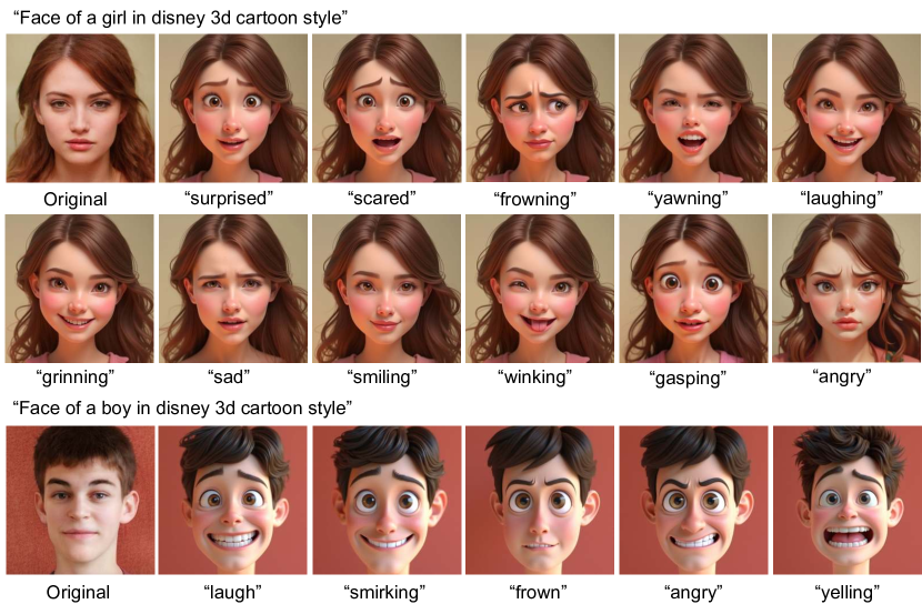
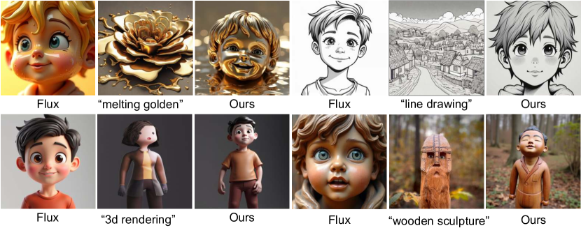
Figure 21 shows stylization based on a single reference style image and 12 different text prompts, covering both living and non-living objects. The generated images contain various style attributes that includes melting elements, golden color, and 3d rendering from the reference style image.

Figure 21: Stylization using a single reference image and various text prompts. Given a reference style image (e.g. “melting golden 3d rendering” at the top) and various text prompts (e.g. “a dwarf in melting golden 3d rendering style”), our method generates images that are consistent with the reference style image and aligned with the given text prompt.

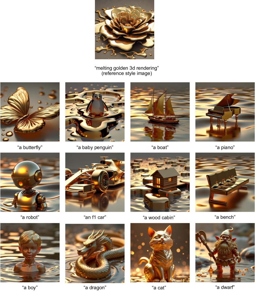
Figure 22 visualizes stylization results based on different reference style images. In this experiment, we use text prompt to describe both the content of the generated image and the style of the given reference style image.

Figure 22: Stylization using a single prompt and various reference style images: “melting golden”, “line drawing”, “3d rendering”, and “wooden sculpture”. Given a style image (e.g. “3d rendering”) and a text prompt (e.g. “face of a boy in 3d rendering style”), our method generates images that are consistent with the reference style image and the text prompt. The standard output from Flux is obtained by disabling our controller, which clearly highlights the importance of the controller.

Figure 23: Interface for human evaluation. Each participant is asked to select their preferred image based on two criteria: realism and faithfulness.

C.6 Human Evaluation

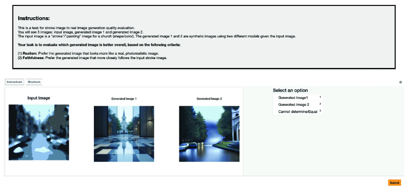
We conduct a user study on the test splits of both LSUN Bedroom and LSUN Church dataset using Amazon Mechanical Turk, with 126 participants in total. As shown in Figure 23, each question was accompanied by an explanation of the task, the question, and the evaluation criteria. Participants were shown a pair of stroke-to-image outputs from different models, in random order, along with the input stroke image. They were asked to select one of three options based on their preference using the following two criteria:

1. Realism: which of these two images look more like a real, photorealistic image?

2. Faithfulness: which of these two images match more closely to the input stroke image?

We collect 3 responses per question. With 300 images in the test dataset and 10 pairwise comparisons, we gathered 9,000 responses for this evaluation. The example in Figure 23 is for the LSUN Church dataset; for LSUN Bedroom dataset, we simply replace the word “church” to “bedroom” in the instructions.

C.7 Generative Modeling using Rectified Stochastic Differential Equations

In Figure 24, we compare images generated by Flux (an ODE-based sampler (19)). The similarity between the images generated by the ODE and SDE versions of Flux strengthens the practical significance of our theoretical results (§3).

Figure 24: T2I generation using rectified SDE (22) for different number of discretization steps marked along the X-axis. The stochastic equivalent sampler FluxSDE generates samples visually comparable to FluxODE at different levels of discretization.

References

- Albergo et al. (2023) Michael S Albergo, Nicholas M Boffi, and Eric Vanden-Eijnden. Stochastic interpolants: A unifying framework for flows and diffusions. arXiv preprint arXiv:2303.08797, 2023.
- Albergo & Vanden-Eijnden (2023) Michael Samuel Albergo and Eric Vanden-Eijnden. Building normalizing flows with stochastic interpolants. In The Eleventh International Conference on Learning Representations, 2023.
- Anderson (1982) Brian D.O. Anderson. Reverse-time diffusion equation models. Stochastic Processes and their Applications, 12(3):313–326, 1982.
- Basar et al. (2020) Tamer Basar, Sean Meyn, and William R Perkins. Lecture notes on control system theory and design. arXiv preprint arXiv:2007.01367, 2020.
- Beniaguev (2022) David Beniaguev. Synthetic faces high quality (sfhq) dataset, 2022. URL https://github.com/SelfishGene/SFHQ-dataset.
- Brack et al. (2024) Manuel Brack, Felix Friedrich, Katharia Kornmeier, Linoy Tsaban, Patrick Schramowski, Kristian Kersting, and Apolinário Passos. Ledits++: Limitless image editing using text-to-image models. In Proceedings of the IEEE/CVF Conference on Computer Vision and Pattern Recognition, pp. 8861–8870, 2024.
- Brooks et al. (2023) Tim Brooks, Aleksander Holynski, and Alexei A Efros. Instructpix2pix: Learning to follow image editing instructions. In Proceedings of the IEEE/CVF Conference on Computer Vision and Pattern Recognition, pp. 18392–18402, 2023.
- Couairon et al. (2023) Guillaume Couairon, Jakob Verbeek, Holger Schwenk, and Matthieu Cord. Diffedit: Diffusion-based semantic image editing with mask guidance. In ICLR 2023 (Eleventh International Conference on Learning Representations), 2023.
- Delbracio & Milanfar (2023) Mauricio Delbracio and Peyman Milanfar. Inversion by direct iteration: An alternative to denoising diffusion for image restoration. Transactions on Machine Learning Research, 2023.
- Efron (2011) Bradley Efron. Tweedie’s formula and selection bias. Journal of the American Statistical Association, 106(496):1602–1614, 2011.
- Esser et al. (2024) Patrick Esser, Sumith Kulal, Andreas Blattmann, Rahim Entezari, Jonas Müller, Harry Saini, Yam Levi, Dominik Lorenz, Axel Sauer, Frederic Boesel, et al. Scaling rectified flow transformers for high-resolution image synthesis. In Forty-first International Conference on Machine Learning, 2024.
- Fleming & Rishel (1975) Wendell H Fleming and Raymond W Rishel. Deterministic and stochastic optimal control, volume 1. Springer Science & Business Media, 1975.
- Hertz et al. (2022) Amir Hertz, Ron Mokady, Jay Tenenbaum, Kfir Aberman, Yael Pritch, and Daniel Cohen-or. Prompt-to-prompt image editing with cross-attention control. In The Eleventh International Conference on Learning Representations, 2022.
- Hertz et al. (2023) Amir Hertz, Andrey Voynov, Shlomi Fruchter, and Daniel Cohen-Or. Style aligned image generation via shared attention. arXiv preprint arXiv:2312.02133, 2023.
- Ho et al. (2020) Jonathan Ho, Ajay Jain, and Pieter Abbeel. Denoising diffusion probabilistic models. Advances in Neural Information Processing Systems, 33:6840–6851, 2020.
- Hu et al. (2021) Edward J Hu, Phillip Wallis, Zeyuan Allen-Zhu, Yuanzhi Li, Shean Wang, Lu Wang, Weizhu Chen, et al. Lora: Low-rank adaptation of large language models. In International Conference on Learning Representations, 2021.
- Ju et al. (2023) Xuan Ju, Ailing Zeng, Chenchen Zhao, Jianan Wang, Lei Zhang, and Qiang Xu. Humansd: A native skeleton-guided diffusion model for human image generation. In Proceedings of the IEEE/CVF International Conference on Computer Vision, pp. 15988–15998, 2023.
- Karras et al. (2022) Tero Karras, Miika Aittala, Timo Aila, and Samuli Laine. Elucidating the design space of diffusion-based generative models. Advances in Neural Information Processing Systems, 35:26565–26577, 2022.
- Karras et al. (2024) Tero Karras, Miika Aittala, Jaakko Lehtinen, Janne Hellsten, Timo Aila, and Samuli Laine. Analyzing and improving the training dynamics of diffusion models. In Proceedings of the IEEE/CVF Conference on Computer Vision and Pattern Recognition, pp. 24174–24184, 2024.
- Kim et al. (2022) Gwanghyun Kim, Taesung Kwon, and Jong Chul Ye. Diffusionclip: Text-guided diffusion models for robust image manipulation. In Proceedings of the IEEE/CVF Conference on Computer Vision and Pattern Recognition, pp. 2426–2435, 2022.
- Kwon & Ye (2023) Gihyun Kwon and Jong Chul Ye. Diffusion-based image translation using disentangled style and content representation. In The Eleventh International Conference on Learning Representations, 2023. URL https://openreview.net/forum?id=Nayau9fwXU.
- Lipman et al. (2022) Yaron Lipman, Ricky TQ Chen, Heli Ben-Hamu, Maximilian Nickel, and Matt Le. Flow matching for generative modeling. arXiv preprint arXiv:2210.02747, 2022.
- Liu et al. (2022) Xingchao Liu, Chengyue Gong, et al. Flow straight and fast: Learning to generate and transfer data with rectified flow. In The Eleventh International Conference on Learning Representations, 2022.
- Meng et al. (2022) Chenlin Meng, Yutong He, Yang Song, Jiaming Song, Jiajun Wu, Jun-Yan Zhu, and Stefano Ermon. Sdedit: Guided image synthesis and editing with stochastic differential equations. In International Conference on Learning Representations, 2022.
- Miyake et al. (2023) Daiki Miyake, Akihiro Iohara, Yu Saito, and Toshiyuki Tanaka. Negative-prompt inversion: Fast image inversion for editing with text-guided diffusion models. arXiv preprint arXiv:2305.16807, 2023.
- Mokady et al. (2023) Ron Mokady, Amir Hertz, Kfir Aberman, Yael Pritch, and Daniel Cohen-Or. Null-text inversion for editing real images using guided diffusion models. In Proceedings of the IEEE/CVF Conference on Computer Vision and Pattern Recognition, pp. 6038–6047, 2023.
- Nichol et al. (2022) Alexander Quinn Nichol, Prafulla Dhariwal, Aditya Ramesh, Pranav Shyam, Pamela Mishkin, Bob Mcgrew, Ilya Sutskever, and Mark Chen. Glide: Towards photorealistic image generation and editing with text-guided diffusion models. In International Conference on Machine Learning, pp. 16784–16804. PMLR, 2022.
- Øksendal (2003) Bernt Øksendal. Stochastic differential equations. Springer, 2003.
- Peebles & Xie (2023) William Peebles and Saining Xie. Scalable diffusion models with transformers. In Proceedings of the IEEE/CVF International Conference on Computer Vision, pp. 4195–4205, 2023.
- Pernias et al. (2024) Pablo Pernias, Dominic Rampas, Mats Leon Richter, Christopher Pal, and Marc Aubreville. Würstchen: An efficient architecture for large-scale text-to-image diffusion models. In The Twelfth International Conference on Learning Representations, 2024. URL https://openreview.net/forum?id=gU58d5QeGv.
- Podell et al. (2023) Dustin Podell, Zion English, Kyle Lacey, Andreas Blattmann, Tim Dockhorn, Jonas Müller, Joe Penna, and Robin Rombach. Sdxl: Improving latent diffusion models for high-resolution image synthesis. In The Twelfth International Conference on Learning Representations, 2023.
- Radford et al. (2021) Alec Radford, Jong Wook Kim, Chris Hallacy, Aditya Ramesh, Gabriel Goh, Sandhini Agarwal, Girish Sastry, Amanda Askell, Pamela Mishkin, Jack Clark, et al. Learning transferable visual models from natural language supervision. In International conference on machine learning, pp. 8748–8763. PMLR, 2021.
- Ramesh et al. (2021) Aditya Ramesh, Mikhail Pavlov, Gabriel Goh, Scott Gray, Chelsea Voss, Alec Radford, Mark Chen, and Ilya Sutskever. Zero-shot text-to-image generation. In International Conference on Machine Learning, pp. 8821–8831. PMLR, 2021.
- Ramesh et al. (2022) Aditya Ramesh, Prafulla Dhariwal, Alex Nichol, Casey Chu, and Mark Chen. Hierarchical text-conditional image generation with clip latents. arXiv preprint arXiv:2204.06125, 2022.
- Rombach et al. (2022) Robin Rombach, Andreas Blattmann, Dominik Lorenz, Patrick Esser, and Björn Ommer. High-resolution image synthesis with latent diffusion models. In Proceedings of the IEEE/CVF Conference on Computer Vision and Pattern Recognition, pp. 10684–10695, 2022.
- Rout et al. (2023a) Litu Rout, Advait Parulekar, Constantine Caramanis, and Sanjay Shakkottai. A theoretical justification for image inpainting using denoising diffusion probabilistic models. arXiv preprint arXiv:2302.01217, 2023a.
- Rout et al. (2023b) Litu Rout, Negin Raoof, Giannis Daras, Constantine Caramanis, Alexandros G Dimakis, and Sanjay Shakkottai. Solving inverse problems provably via posterior sampling with latent diffusion models. In Thirty-seventh Conference on Neural Information Processing Systems, 2023b. URL https://openreview.net/forum?id=XKBFdYwfRo.
- Rout et al. (2024a) Litu Rout, Yujia Chen, Abhishek Kumar, Constantine Caramanis, Sanjay Shakkottai, and Wen-Sheng Chu. Beyond first-order tweedie: Solving inverse problems using latent diffusion. In 2024 IEEE/CVF Conference on Computer Vision and Pattern Recognition, 2024a.
- Rout et al. (2024b) Litu Rout, Yujia Chen, Nataniel Ruiz, Abhishek Kumar, Constantine Caramanis, Sanjay Shakkottai, and Wen-Sheng Chu. Rb-modulation: Training-free personalization of diffusion models using stochastic optimal control. arXiv preprint arXiv:2405.17401, 2024b.
- Ruiz et al. (2023) Nataniel Ruiz, Yuanzhen Li, Varun Jampani, Yael Pritch, Michael Rubinstein, and Kfir Aberman. Dreambooth: Fine tuning text-to-image diffusion models for subject-driven generation. In Proceedings of the IEEE/CVF Conference on Computer Vision and Pattern Recognition, pp. 22500–22510, 2023.
- Ruiz et al. (2024) Nataniel Ruiz, Yuanzhen Li, Varun Jampani, Wei Wei, Tingbo Hou, Yael Pritch, Neal Wadhwa, Michael Rubinstein, and Kfir Aberman. Hyperdreambooth: Hypernetworks for fast personalization of text-to-image models. In Proceedings of the IEEE/CVF Conference on Computer Vision and Pattern Recognition, pp. 6527–6536, 2024.
- Saharia et al. (2022) Chitwan Saharia, William Chan, Huiwen Chang, Chris A. Lee, Jonathan Ho, Tim Salimans, David J. Fleet, and Mohammad Norouzi. Palette: Image-to-image diffusion models, 2022.
- Sohl-Dickstein et al. (2015) Jascha Sohl-Dickstein, Eric Weiss, Niru Maheswaranathan, and Surya Ganguli. Deep unsupervised learning using nonequilibrium thermodynamics. In Francis Bach and David Blei (eds.), Proceedings of the 32nd International Conference on Machine Learning, volume 37 of Proceedings of Machine Learning Research, pp. 2256–2265, Lille, France, 07–09 Jul 2015. PMLR. URL https://proceedings.mlr.press/v37/sohl-dickstein15.html.
- Song et al. (2021a) Jiaming Song, Chenlin Meng, and Stefano Ermon. Denoising diffusion implicit models. In International Conference on Learning Representations, 2021a. URL https://openreview.net/forum?id=St1giarCHLP.
- Song & Ermon (2019) Yang Song and Stefano Ermon. Generative modeling by estimating gradients of the data distribution. Advances in Neural Information Processing Systems, 32, 2019.
- Song et al. (2021b) Yang Song, Jascha Sohl-Dickstein, Diederik P Kingma, Abhishek Kumar, Stefano Ermon, and Ben Poole. Score-based generative modeling through stochastic differential equations. In International Conference on Learning Representations, 2021b. URL https://openreview.net/forum?id=PxTIG12RRHS.
- Tumanyan et al. (2023) Narek Tumanyan, Michal Geyer, Shai Bagon, and Tali Dekel. Plug-and-play diffusion features for text-driven image-to-image translation. In Proceedings of the IEEE/CVF Conference on Computer Vision and Pattern Recognition, pp. 1921–1930, 2023.
- Tzen & Raginsky (2019) Belinda Tzen and Maxim Raginsky. Theoretical guarantees for sampling and inference in generative models with latent diffusions. In Conference on Learning Theory, pp. 3084–3114. PMLR, 2019.
- Wang et al. (2017) Limin Wang, Sheng Guo, Weilin Huang, Yuanjun Xiong, and Yu Qiao. Knowledge guided disambiguation for large-scale scene classification with multi-resolution cnns. IEEE Transactions on Image Processing, 26(4):2055–2068, 2017.
- Wu & De la Torre (2023) Chen Henry Wu and Fernando De la Torre. A latent space of stochastic diffusion models for zero-shot image editing and guidance. In Proceedings of the IEEE/CVF International Conference on Computer Vision, pp. 7378–7387, 2023.
- Zhang & Chen (2022) Qinsheng Zhang and Yongxin Chen. Path integral sampler: A stochastic control approach for sampling. In International Conference on Learning Representations, 2022. URL https://openreview.net/forum?id=_uCb2ynRu7Y.