Singular Twist Waves in Chromonic Liquid Crystals

Abstract

Chromonic liquid crystals are lyotropic nematic phases whose applications span from food to drug industries. It has recently been suggested that the elastic energy density governing the equilibrium distortions of these materials may be quartic in the measure of twist. Here we show that the non-linear twist-wave equation associated with such an energy has smooth solutions that break down in a finite time, giving rise to the formation of a shock wave, under rather generic assumptions on the initial profile. The critical time at which smooth solutions become singular is estimated analytically with an accuracy that numerical calculations for a number of exemplary cases prove to be satisfactory.

I Introduction

Lyotropic liquid crystals phases arise in colloidal solutions (mostly aqueous) when the concentration of the solute is sufficiently high or the temperature is sufficiently low. Chromonic liquid crystals (CLCs) are special lyotropic phases with potential applications in life sciences [1, 2, 3, 4]. These materials are constituted by plank-shaped molecules that arrange themselves in stacks when dissolved in water. For sufficiently high concentrations or low temperatures, the constituting stacks give rise to an ordered phase, either nematic or columnar [5, 6, 7, 8, 9]. Here, we shall only be concerned with the nematic phase, in which the elongated microscopic constituents of the material display a certain degree of orientational order, while their centres of mass remain disordered. Numerous substances have a CLC phase; these include organic dyes (especially those common in food industry), drugs, and oligonucleotides.

The classical quadratic elastic theory of Oseen [10] and Frank [11] was proved to have potentially paradoxical consequences when applied to free-boundary problems, such as those concerning the equilibrium shape of CLC droplets surrounded by their isotropic phase [12]. To remedy this state of affairs, a quartic elastic theory was proposed for CLCs in [13], which alters the Oseen-Frank energy density by the addition of a single quartic term in the twist measure of nematic distortion. Preliminary experimental confirmations of the validity of this theory are presented in [14, 15, 16].

All these applications of the quartic elastic theory fall in the realm of statics. In this paper, we move a step forward and explore the dynamical consequences of this theory. To this end, in Sect. II we present a general dynamical setting, indeed far more general than it would strictly be fit for our purposes, as we also contemplate the possibility that the scalar degree of order $s$ be variable in space and time like the nematic director $\bm{n}$.

In Sect. III, we recall the basic features of the elastic quartic twist theory and in Sect. IV we write the general dynamical equations in the special case where the fluid remains quiescent, while $\bm{n}$ exhibits a single distortion mode, the twist, which is described by a single scalar function $w$ in a single spatial variable $x$ and time $t$. In Sect. V, for the conservative case, which is the only one considered in this paper, $w$ is found to obey a non-linear wave equation with propagation velocity that depends on the spatial derivative $w_{,x}$. Even if the initial profile $w_{0}$ is smooth, in its evolution $w$ is bound to brood singularities that erupt in a finite time $t^{\ast}$, at which second derivatives become unbounded and first derivatives develop discontinuities. This is when a smooth wave breaks down and a shock wave emerges from it, a typical non-linear phenomenon that the Oseen-Frank quadratic theory could not embrace.

As also shown in Sect. V, the classical theory of hyperbolic equations does not suffice to our needs, for the wave velocity is not in a standard form. Building on more recent analytical results, we construct the mathematical framework that serves our purposes. Thus, in Sect. VI, we prove that under mild assumptions on the initial twist profile $w_{0}$, all smooth solutions $w$ to the wave equation do indeed break down, and we give an upper estimate for the critical time $t^{\ast}$ that numerical solutions illustrated in Sect. VII prove to be quite accurate.

Finally, in Sect. VIII, we collect the conclusions of our study and comment on possible ways to extend it. The paper is closed by two appendices, where we present mathematical details that are needed to make our development self-contained, but which would disrupt the reader’s attention, if placed in the main body of the paper.

II Generalized Ericksen-Leslie Theory

Here, mainly following [17] (and Chapt. 3 of [18]), we present the general dynamical theory of nematic liquid crystals that extends the early formulation of the foundation papers [19, 20, 21, 22, 23, 24], also summarized in [25]. Although in the rest of the paper this theory will not be employed in its full-fledged version, it provides the general framework within which our study is developed; it would serve as the natural environment for possible future extensions. As in the pioneering work of Ericksen [26], both macro- and micro-inertia of the motion will systematically be included in the picture.

The local molecular organization of nematic liquid crystals is described by a director field $\bm{n}$, representing the average orientation of the (elongated) molecular aggregates that constitute the material, and a scalar field $s$, the degree of orientation, which vanishes where the orientational order is lost. Nematic liquid crystals are commonly described as incompressible, dissipative, ordered fluids: a continuum theory capable of describing their dynamics must primarily model the coupled evolution of the orientation of the microscopic constituents, their degree of order, and the macroscopic flow, described by $\bm{n}$, $s$, and the velocity field $\bm{v}$, respectively.

In the general variational approach proposed in [18], which we also adopt here, the dynamical equations are derived from a Lagrange-Rayleigh dissipation principle. Letting $\mathscr{B}_{t}$ be the smooth region in three-dimensional space occupied at the time $t$ by a generic sub-body during its motion, we denote by $(\bm{t},\bm{c},K)$ the system of generalized tractions and by $(\bm{b},\bm{k},L)$ the system of generalized body forces expending power against the generalized velocities $(\bm{v},\dot{\bm{n}},\dot{s})$, on the boundary $\partial\mathscr{B}_{t}$ and in the interior $\mathring{\mathscr{B}}_{t}$, respectively. A standard localization argument implies the following evolution equations (see Sect. 3.2 of [18] for more details about the general method),

$$\rho\dot{\bm{v}}=\bm{b}+\operatorname{div}\bm{\mathrm{T}},$$ (1a)

$$\sigma\ddot{\bm{n}}+\frac{\partial R}{\partial\accentset{\circ}{\bm{n}}}+\frac{\partial W}{\partial\bm{n}}-\operatorname{div}\left(\frac{\partial W}{\partial\nabla\bm{n}}\right)-\bm{k}=\mu\bm{n},$$ (1b)

$$\frac{\partial W}{\partial s}-\operatorname{div}\frac{\partial W}{\partial\nabla s}+\frac{\partial R}{\partial\dot{s}}=L,$$ (1c)

in $\mathscr{B}_{t}$, and

$$\bm{t}=\bm{\mathrm{T}}\bm{\nu},$$ (2a)

$$\bm{c}=\frac{\partial W}{\partial\nabla\bm{n}}\bm{\nu},$$ (2b)

$$\frac{\partial W}{\partial\nabla s}\cdot\bm{\nu}=K,$$ (2c)

on $\partial\mathscr{B}_{t}$, where a superimposed dot denotes the material time derivative, $\rho$ is the mass density, $\sigma$ is the density of (microscopic) moment of inertia, $\mu$ is a Lagrange multiplier which ensures that $\bm{n}$ obeys the constraint $\bm{n}\cdot\bm{n}\equiv 1$, $W$ is the elastic free-energy density, $R$ is the Rayleigh dissipation function, and $\bm{\nu}$ is the outer unit normal to $\partial\mathscr{B}_{t}$.

Typically, for liquid crystals of small molecular weight, $\sigma$ is set equal to zero in the equations that govern the evolution of $\bm{n}$, indicating that no inertial torque acts on the director. In these cases, the microkinetic energy associated with the motion of $\bm{n}$ is systematically neglected in favor of the predominant macroscopic kinetic energy $\frac{1}{2}\rho\bm{v}^{2}$ of the fluid. However, for lyotropic liquid crystals, particularly for CLCs, this assumption may be inaccurate, as in these fluids large molecular complexes act as elementary constituents of the material, making it important to consider inertia or delays in molecular reorientation.

For nematic materials, the elastic free-energy density $W$ is taken to be a frame-indifferent function $W=W(s,\nabla s,\bm{n},\nabla\bm{n})$ that is positive definite,

$$W(s,\nabla s,\bm{n},\nabla\bm{n})\geq W(s,\bm{0},\bm{n},\bm{0})=W_{0}(s)\geq 0,$$ (3)

and reflects the nematic symmetry,

$$W(s,\nabla s,\bm{n},\nabla\bm{n})=W(s,\nabla s,-\bm{n},-\nabla\bm{n}).$$ (4)

The Rayleigh dissipation function $R$ plays a central role in the dynamics of dissipative fluids. Here it is taken as a quadratic function in the (indifferent) measures of dissipation. These latter are the stretching tensor $\mathbf{D}$, that is, the symmetric part of the velocity gradient $\nabla\bm{v}$, the corotational time derivative $\mathring{\bm{n}}$ of the director,

$$\mathring{\bm{n}}:=\dot{\bm{n}}-\mathbf{W}\bm{n},$$ (5)

where $\mathbf{W}$ is the vorticity tensor, that is, the skew part of $\nabla\bm{v}$, and finally the material time derivative of the scalar order parameter, $\dot{s}$. We thus write $R$ as the following function,

$$R(s,\bm{n};\bm{\mathrm{D}},\accentset{\circ}{\bm{n}},\dot{s})=\beta_{1}\dot{s}\bm{n}\cdot\bm{\mathrm{D}}\bm{n}+\frac{\beta_{2}}{2}\dot{s}^{2}+\frac{\gamma_{1}}{2}\accentset{\circ}{\bm{n}}^{2}+\gamma_{2}\accentset{\circ}{\bm{n}}\cdot\bm{\mathrm{D}}\bm{n}+\frac{\gamma_{3}}{2}(\bm{\mathrm{D}}\bm{n})^{2}+\frac{\gamma_{4}}{2}(\bm{n}\cdot\bm{\mathrm{D}}\bm{n})^{2}+\frac{\gamma_{5}}{2}\operatorname{tr}{\bm{\mathrm{D}}}^{2},$$ (6)

where the coefficients $\beta$’s and $\gamma$’s are the generalized viscosities, functions of $s$ subject to the requirement that $R$ in (6) be positive semidefinite. In particular, the rotational (or twist) viscosity $\gamma_{1}$ must satisfy the inequality $\gamma_{1}\geq 0$.

Equation (1a) expresses the balance of linear momentum, while (1b) and (1c) are additional equations governing the evolution of $\bm{n}$ and $s$. It can be shown reasoning as in [18, p. 198] that the balance equation of rotational momentum is a consequence of the frame-indifference of the function $W$ and equation (1b).

The Cauchy stress tensor $\mathbf{T}$ comprises both elastic and viscous components, as is clear from the following formula (see [18, p. 197]),

$$\mathbf{T}=-p\mathbf{I}\underbrace{-\left(\nabla\bm{n}\right)^{\mathsf{T}}\frac{\partial W}{\partial\nabla\bm{n}}-\nabla s\otimes\frac{\partial W}{\partial\nabla s}}_{\text{elastic stress}}+\underbrace{\frac{1}{2}\left(\bm{n}\otimes\frac{\partial R}{\partial\mathring{\bm{n}}}-\frac{\partial R}{\partial\mathring{\bm{n}}}\otimes\bm{n}\right)+\frac{\partial R}{\partial\mathbf{D}}}_{\text{viscous stress}},$$ (7)

where $p$ is the pressure, an unknown function representing the Lagrange multiplier that enforces the incompressibility constraint, $\operatorname{div}\bm{v}\equiv 0$.

The generalized Ericksen-Leslie equations recalled above afford a conveniently simplified description of defects, which can be identified with the regions in space (typically, points or lines) where $s$ vanishes. In the dynamical problem that we shall be concerned with, the director field is unlikely to develop defects; it is instead expected to develop another type of singularity, not in $\bm{n}$ itself, but both in its gradient $\nabla\bm{n}$ and time derivative $\dot{\bm{n}}$. For this reason, the assumption that

$$s\equiv s_{0}$$ (8)

will be adopted in the rest of the paper. Under this assumption, which requires that both $K\equiv 0$ and $L\equiv 0$ for consistency, equations (1c) and (2c) will be void.

In the following section, we shall derive the form of elastic free-energy density $W=W(\bm{n},\nabla\bm{n})$ appropriate for CLCs; we shall see then in Sect. IV how a type of non-linearity arises there that makes the twist waves generated in CLCs differ from the solitons studied in ordinary nematics.

The solitons mainly involved in liquid crystals are solutions to an appropriate form of the (dissipative) sine-Gordon equation. They were also called walls in the first, pioneering studies [28, 29, 30, 31, 32]. These usually turned out to be of small amplitude (and so, difficult to observe) and sustained by an external magnetic field. Later works [33, 34, 35, 36] then proved the existence of solitons in the director field driven by a hydrodynamic flow; these were also governed by a sine-Gordon equation, but easier to observe experimentally. At variance with the case treated here, in that equation the non-linearity manifested itself in the forcing term, while the differential part remained linear.

III Energetics of Chromonics

Here, following closely [16], we recall the quartic elastic theory for CLCs adopted in this paper. What makes chromonic nematics differ from ordinary ones is the ground state of their distortion: a double twist for the former, a uniform field (along any direction) for the latter. We now explore this difference in more detail.

Like Selinger [38], we write the elastic energy density of the Oseen-Frank theory [10, 11] in an equivalent form,

$$W_{\mathrm{OF}}(\bm{n},\nabla\bm{n})=\frac{1}{2}(K_{11}-K_{24})S^{2}+\frac{1}{2}(K_{22}-K_{24})T^{2}+\frac{1}{2}K_{33}B^{2}+2K_{24}q^{2},$$ (9)

where $S:=\operatorname{div}\bm{n}$ is the splay, $T:=\bm{n}\cdot\operatorname{curl}\bm{n}$ is the twist, $B^{2}:=\bm{b}\cdot\bm{b}$ is the square modulus of the bend vector $\bm{b}:=\bm{n}\times\operatorname{curl}\bm{n}$, and $q>0$ is the octupolar splay [39] derived from the following equation

$$2q^{2}=\operatorname{tr}(\nabla\bm{n})^{2}+\frac{1}{2}T^{2}-\frac{1}{2}S^{2}.$$ (10)

Since $(S,T,B,q)$ are independent distortion measures, it easily follows from (9) that $W_{\mathrm{OF}}$ is positive semi-definite whenever

$$K_{11}\geqq K_{24}\geqq 0,$$ (11a)

$$K_{22}\geqq K_{24}\geqq 0,$$ (11b)

$$K_{33}\geqq 0,$$ (11c)

which are the celebrated Ericksen’s inequalities [40]. If these inequalities are satisfied in strict form, the global ground state of $W_{\mathrm{OF}}$ is attained on any uniform director field, characterized by

$$S=T=B=q=0,$$ (12)

which designates the ground state of ordinary nematics.

CLCs are characterized by a different ground state, which we call a double twist, one where all distortion measures vanish, but $T$. Here, we adopt the terminology proposed by Selinger [41] (see also [42]) and distinguish between single and double twists. The former is characterized by

$$S=0,\quad B=0,\quad T=\pm 2q,$$ (13)

which designates a director distortion capable of filling uniformly the whole space [43]. For the Oseen-Frank theory to accommodate such a ground state, inequality (11b) must be replaced by $K_{24}\geqq K_{22}\geqq 0$, but this comes at the price of making $W_{\mathrm{OF}}$ unbounded below [44].

The essential feature of the quartic twist theory proposed in [13] is to envision a double twist (with two equivalent chiral variants) as ground state of CLCs in three-dimensional space,

$$S=0,\quad T=\pm T_{0},\quad B=0,\quad q=0.$$ (14)

The degeneracy of the ground double twist in (14) arises from the achiral nature of the molecular aggregates that constitute these materials, which is reflected in the lack of chirality of their condensed phases.

The elastic stored energy must equally penalize both ground chiral variants. Our minimalist proposal to achieve this goal was to add a quartic twist term to the Oseen-Frank stored-energy density,

$$W_{\mathrm{QT}}(\bm{n},\nabla\bm{n}):=\frac{1}{2}(K_{11}-K_{24})S^{2}+\frac{1}{2}(K_{22}-K_{24})T^{2}+\frac{1}{2}K_{23}B^{2}+2K_{24}q^{2}+\frac{1}{4}K_{22}a^{2}T^{4},$$ (15)

where $a$ is a characteristic length. $W_{\mathrm{QT}}$ is bounded below whenever

$$K_{11}\geqq K_{24}\geqq 0,$$ (16a)

$$K_{24}\geqq K_{22}\geqq 0,$$ (16b)

$$K_{33}\geqq 0.$$ (16c)

If these inequalities hold, as we shall assume here, then $W_{\mathrm{QT}}$ is minimum at the degenerate double twist (14) characterized by

$$T_{0}:=\frac{1}{a}\sqrt{\frac{K_{24}-K_{22}}{K_{22}}}.$$ (17)

Here, we shall treat $a$ as a phenomenological parameter to be determined experimentally.

IV Twist Waves in Chromonics

Twist waves in nematic liquid crystals were fist studied by Ericksen in [26]. They are special solutions to the hydrodynamic equations under the assumption that the flow velocity $\bm{v}$ vanishes: this implies that the motion of the director induces no backflow. The governing one-dimensional wave equation derived in [26] presumes that no extrinsic body forces or couples act on the system, and that the material occupies the whole space, assumptions that will be retained in this paper.

Since $\bm{v}\equiv\bm{0}$, $\mathbf{D}\equiv\mathbf{0}$ and both the material and corotational derivatives of $\bm{n}$ reduce to its partial time derivative $\partial_{t}\bm{n}$. Moreover, by combining (6), (7), and (8), we readily give the Cauchy stress tensor $\mathbf{T}$ the following form

$$\mathbf{T}=-p\mathbf{I}-\left(\nabla\bm{n}\right)^{\mathsf{T}}\frac{\partial W}{\partial\nabla\bm{n}}+\mu_{2}\partial_{t}\bm{n}\otimes\bm{n}+\mu_{3}\bm{n}\otimes\partial_{t}\bm{n},$$ (18)

where

$$\mu_{2}:=\frac{1}{2}(\gamma_{2}-\gamma_{1})\quad\text{and}\quad\mu_{3}:=\frac{1}{2}(\gamma_{2}+\gamma_{1}).$$ (19)

In the absence of body forces and couples, the balance equations in (1) thus reduce to

$$\operatorname{div}\mathbf{T}=\bm{0},$$ (20a)

$$\sigma\partial_{tt}\bm{n}+\gamma_{1}\partial_{t}\bm{n}+\frac{\partial W}{\partial\bm{n}}-\operatorname{div}\left(\frac{\partial W}{\partial\nabla\bm{n}}\right)=\mu\bm{n}.$$ (20b)

Letting $\bm{n}$ be represented in a Cartesian frame $(\bm{e}_{x},\bm{e}_{y},\bm{e}_{z})$ as

$$\bm{n}=\cos w\bm{e}_{y}+\sin w\bm{e}_{z},$$ (21)

where $w=w(t,x)$ denotes the twist angle for $(t,x)\in[0,\infty)\times\mathbb{R}$ and setting $W=W_{\mathrm{QT}}$, we easily see that $T$ and $q$ are the only (related) distortion measures that do not vanish,

$$S=0,\quad T=-w_{,x},\quad B=0,\quad 2q^{2}=\frac{1}{2}T^{2},$$ (22)

the governing equations (20) are equivalent to

$$\sigma w_{,tt}-K_{22}\left(1+3a^{2}w_{,x}^{2}\right)w_{,xx}=-\gamma_{1}w_{,t},$$ (23)

$$\mu=-\sigma w_{,t}^{2}+K_{22}w_{,x}^{2}\left(1+a^{2}w_{,x}^{2}\right),$$ (24)

and

$$p=-K_{22}w_{,x}^{2}(1+a^{2}w_{,x}^{2})+p_{0}(t)=-T\frac{\partial W_{\mathrm{QT}}}{\partial T}+p_{0}(t),$$ (25)

where $p_{0}(t)$ is an arbitrary function of time. While equations (25) and (24) determine the Lagrange multipliers associated with the constraints enforced by the theory, (23) is the genuine evolution equation of the system, whose solutions thus provide a complete solution to the governing equations.

The following sections will be devoted to the analysis of a special instance of equation (23). The molecular inertia $\sigma$ is responsible for its hyperbolic character: equation (23) becomes parabolic if $\sigma$ vanishes.

IV.1 Non-dimensional form

We find it convenient to rescale lengths to $\sqrt{3}a$ and times to the characteristic time

$$\tau:=\sqrt{3}a\sqrt{\frac{\sigma}{K_{22}}}.$$ (26)

Keeping the original names for the rescaled variables $(t,x)$, we write (23) as

$$w_{,tt}-Q^{2}(w_{,x})w_{,xx}=-\lambda w_{,t}\quad\text{for}\quad(t,x)\in[0,+\infty)\times\mathbb{R},$$ (27)

where $Q(\xi)$, the positive root of

$$Q^{2}(\xi):=1+\xi^{2},$$ (28)

is the dimensionless wave velocity and $\lambda$ is a dimensionless damping parameter defined as

$$\lambda:=a\gamma_{1}\sqrt{\frac{3}{\sigma K_{22}}}.$$ (29)

In our scaling, the molecular inertia $\sigma$ affects both $\lambda$ and $\tau$, making the former larger and the latter smaller when it is decreased, so that the director evolution becomes overdamped and (correspondingly) its hyperbolic character applies to an ever shrinking time scale.

IV.2 Parameter Estimates

Here we estimate both $\lambda$ and $\tau$ for actual CLCs. For the former estimate, we start from the rotational viscosity $\gamma_{1}$ of SSY and DSCG measured in [45]. Specifically, at room temperature and for various concentrations, Fig. $3$a in [45] shows that

$$\gamma_{1}^{\mathrm{SSY}}\sim 1\mathrm{Pa}\,\mathrm{s},\quad\gamma_{1}^{\mathrm{DSCG}}\sim 10^{2}\mathrm{Pa}\,\mathrm{s}.$$ (30)

These measurements indicate that for SSY and DSCG $\gamma_{1}$ is approximately two and four orders of magnitude greater, respectively, than that of the thermotropic 5CB when the scalar degree of order is $s_{0}\sim 1$.

The estimate of $\sigma$ for CLCs is more uncertain. Since it is expected to be proportional to the square of the average length of molecular aggregates, precisely like $\gamma_{1}$, we assume that for SSY and DSCG $\sigma$ is accordingly two and four orders of magnitude greater, respectively, than the typical value for a thermotropic liquid crystal. From the measurements in [46] for MBBA, $\sigma$ is estimated to be of order $10^{-13}\mathrm{kg}/\mathrm{m}$; thus, we take

$$\sigma^{\mathrm{SSY}}\sim 10^{-11}\mathrm{kg}/\mathrm{m}\quad\text{and}\quad\sigma^{\mathrm{DSCG}}\sim 10^{-9}\mathrm{kg}/\mathrm{m}.$$ (31)

In previous studies [13, 14, 16, 15], we estimated the phenomenological length $a$ from experimental data for CLCs under different spatial confinements. On the basis of such preliminary experimental evidence, we find that $a\sim 10\mu\mathrm{m}$ could be a sensible estimate, at least in ordinary physical conditions. Taking $K_{22}\sim 1\mathrm{pN}$ as a typical order of magnitude for the twist elastic constant of CLCs [47], we obtain the following estimate of $\lambda$ for both SSY and DSCG solutions in the deep nematic phase (that is, for $s_{0}\sim 1$),

$$\lambda^{\mathrm{SSY}}\approx\lambda^{\mathrm{DSCG}}\approx 5\times 10^{6},$$ (32)

which is a very large number. Correspondingly, the characteristic scaling time $\tau$ is estimated as follows for both solutions,

$$\tau^{\mathrm{SSY}}\sim 10^{-5}\mathrm{s}\quad\text{and}\quad\tau^{\mathrm{DSCG}}\sim 10^{-4}\mathrm{s}.$$ (33)

Thus, in ordinary physical conditions and concentrations typical of the deep nematic phase, the parabolic character of (27) prevails at typical experimental time scales. However, its hyperbolic character can manifest itself if we approach the nematic-to-isotropic phase transition, where the scalar order parameter $s_{0}$ approaches $0$. As also remarked in [48, 49], $\sigma$, being determined by the geometric structure of molecular aggregates, is independent of $s_{0}$, whereas both $\gamma_{1}$ and $K_{22}$ scale like $s_{0}^{2}$. Thus,

$$\lambda\propto s_{0}\quad\text{and}\quad\tau\propto\frac{1}{s_{0}},$$ (34)

and making $s_{0}$ small we can neglect $\lambda$ in (27) and inflate the time interval where the hyperbolic character of this equation prevails.

In the rest of the paper, we shall set $\lambda=0$ and study systematically the non-dissipative limit of equation (27). The physical relevance of our conclusions for actual CLCs will be higher as closer these materials approach their nematic-isotropic transition.

V Mathematical Methodology

In this section, we study the following global Cauchy problem for the function $w(t,x)$,

$$w_{,tt}-Q^{2}(w_{,x})w_{,xx}=0 (t,x)\in[0,+\infty)\times\mathbb{R}$$ for , (35a)

$$w(0,x)=w_{0}(x) x\in\mathbb{R}$$ for , (35b)

$$w_{,t}(0,x)=0 x\in\mathbb{R},$$ for (35c)

where $w_{0}$ is a function of class $\mathcal{C}^{2}$ such that $w_{0}^{\prime}$ is not constant, but bounded, and $Q$ is the function defined in (28).

Remark 1.

Since $Q(\xi)>0$ for all $\xi\in\mathbb{R}$, we may say that equation (35a) is strictly hyperbolic, but since $Q^{\prime}(0)=0$, it is not genuinely nonlinear (according to the definition given in [50, p. 15]).

We are mainly interested in providing conditions sufficient to guarantee that the solution $w$ to (35) breaks down in a finite time, meaning that some second derivatives of $w$ become infinite. Such a breakdown ushers the formation of a twist shock wave, where discontinuities in the first derivatives $w_{,x}$ and $w_{,t}$ arise across a plane traveling in time (with law $x=x_{0}(t)$), while $w$ remains continuous. We shall not study these waves here; we shall be contented to determine initial conditions that necessarily lead to their formation.

The study of twist shock waves in quiescent liquid crystals has a long and interesting history starting with the works of Ericksen [51, 25], but it is limited to weak shocks, for which the traveling discontinuities occur either in the second derivatives of the twist angle $w$ (acceleration shock waves) or even in higher derivatives (weaker shock waves).

Acceleration and weaker shock waves behave quite differently in liquid crystals if the elastic energy density $W$ grows faster than $T^{2}$, as is the case for $W_{\mathrm{QT}}$ in (15). As shown in [52, 53], whenever $W$ is more than quadratic in $T$, weaker shock waves decay in a short time, whereas acceleration shock waves may survive for longer times and possibly evolve into ordinary shock waves. Conversely, when $W$ is at most quadratic in $T$, both acceleration and weaker shock waves decay in a finite time.

Here, we are considering a different approach to twist shock waves: we describe how they can arise in a finite time from a regular (smooth) solution of system (35). To this end, the quartic growth of $W_{\mathrm{QT}}$ in $T$ suffices to make (35a) non-linear.

The occurrence of ordinary shock waves in one-dimensional director distortions in a quiescent liquid crystal has also been studied in both dissipative [54] and conservative [55, 56] settings. These waves, however, are governed by an equation where the wave velocity $Q$ is a (nonlinear) function of the angle $w$, instead of $w_{,x}$: they are splay-bend waves instead of twist waves, and so they fall outside the scope of this paper.

Equation (35a) that governs conservative twist waves has some antecedents in the literature, which we now briefly recall. It was studied in [57] by applying a general method earlier developed in [58], in the case where

$$Q^{2}(\xi)=(1+\varepsilon\xi)^{\alpha},$$ (36)

with both $\varepsilon$ and $\alpha$ positive parameters. This special form of the wave velocity was suggested by the pioneering numerical study of a discretized non-linear string [59]. While it was proved in [57] that the continuum equation would predict a breakdown of the solution after a time $t^{\ast}=O(1/\varepsilon\alpha)$, the discretized version studied in [59] remained smooth at all times. With yet another method, the breakdown result of [57] was extended in [60] to a general class of positive functions $Q$ such that

$$|Q^{\prime}(\xi)|>0\quad\forall\ \xi\in\mathbb{R}.$$ (37)

Moreover, a deep analysis of solution breakdown was performed in [61] in a complementary case, where $Q$ obeys the following assumptions.

$$Q(\xi)>0,\quad Q(0)=1,\quad\text{and}\quad\operatorname{sgn}(Q^{\prime}(\xi)\xi)=-1\quad\forall\ \xi\neq 0.$$ (38)

Clearly, neither (37) nor (38) apply to the function $Q$ in (28) that occurs in our system (35), for which we thus need newer analytical methods. We found them in the work [62]; they will be recalled and adapted to our needs in the rest of this section.

V.1 Problem Reformulation

We start by considering as independent unknowns the following first-order derivatives,

$$u_{1}(t,x):=w_{,x}(t,x),\quad u_{2}(t,x):=w_{,t}(t,x)$$ (39)

By their use, we transform (35) into a first-order system,

$$u_{1,t}=u_{2,x},$$ (40a)

$$u_{2,t}=Q^{2}(u_{1})u_{1,x}.$$ (40b)

Applying classical methods (see, for example, [63, 61, 64]), we diagonalize system (40) with the aid of Riemann’s invariants $r$ and $\ell$ defined by

$$r(t,x):=u_{2}(t,x)-L(u_{1}(t,x)),$$ (41a)

$$\ell(t,x):=u_{2}(t,x)+L(u_{1}(t,x)),$$ (41b)

where $L$ is an appropriate mapping. It is a simple matter to show that by setting

$$L^{\prime}(u_{1})=Q(u_{1}),$$ (42)

the system (40) can be written as

$$r_{,t}+Qr_{,x}=0 (t,x)\in[0,t_{\ast})\times\mathbb{R}$$ for , (43a)

$$\ell_{,t}-Q\ell_{,x}=0 (t,x)\in[0,t_{\ast})\times\mathbb{R}$$ for , (43b)

where $[0,t_{\ast})$ is the maximal interval of classical existence. For (43) to acquire the desired diagonal form, we need to express $Q$ as a function of $r$ and $\ell$ only. This can be achieved by use of (28) and (41), which lead us to

$$\ell(t,x)-r(t,x)=2L(u_{1})=2\int_{0}^{u_{1}}Q(\xi)\operatorname{d}\!\xi=u_{1}\sqrt{1+u_{1}^{2}}+\operatorname{arcsinh}u_{1},$$ (44)

where we have set $L(0)=0$, with no prejudice for the validity of (42). By inverting (44), we obtain that

$$u_{1}=\widehat{u}_{1}(\eta):=L^{-1}\left(-\frac{1}{2}\eta\right),$$ (45)

where

$$\eta:=r-\ell.$$ (46)

In (43) we can thus formally replace the function $Q(u_{1})$ with

$$k(\eta):=Q(\widehat{u}_{1}(\eta)),$$ (47)

finally arriving at

$$r_{,t}+k(r-\ell)r_{,x}=0 (t,x)\in[0,t_{\ast})\times\mathbb{R}$$ for , (48a)

$$\ell_{,t}-k(r-\ell)\ell_{,x}=0 (t,x)\in[0,t_{\ast})\times\mathbb{R}$$ for , (48b)

subject to the initial conditions

$$r(0,x)=r_{0}(x)=-L(w_{0}^{\prime}(x)),\quad\ell(0,x)=\ell_{0}(x)=L(w_{0}^{\prime}(x))=-r_{0}(x).$$ (48c)

The graphs of both functions $\widehat{u}_{1}(\eta)$ and $k(\eta)$ are illustrated in Fig. 1.

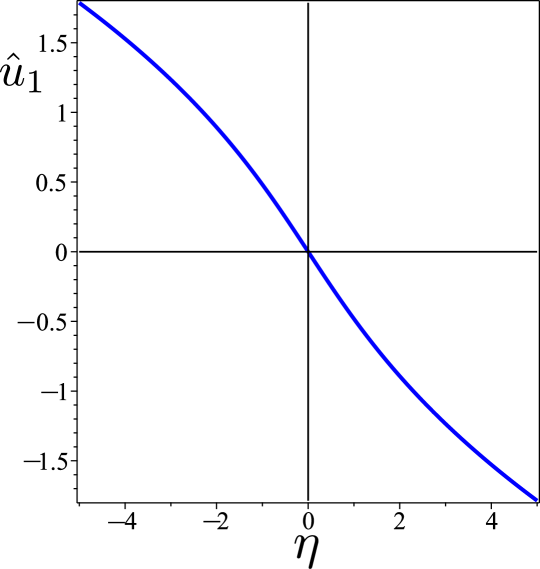
(a) Graphical solution $u_{1}$ of (44) depicted as a function of $\eta$.

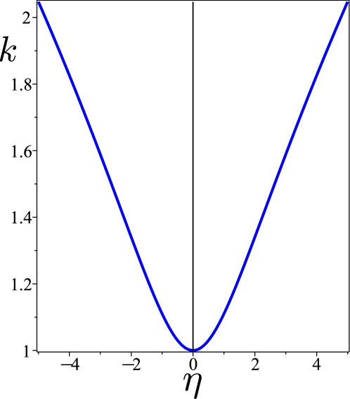
(b) Graph of the function $k$ in (47), illustrating its dependence on $\eta$ through $\widehat{u}_{1}$ defined in (45).

Figure 1: Functions $\widehat{u}_{1}$ and $k$ defined in (45) and (47), respectively, expressed in terms of $\eta:=r-\ell$.

The characteristics of (48) are family of curves $x=x_{1}(t,\alpha)$ and $x=x_{2}(t,\beta)$, indexed in $\alpha,\,\beta\in\mathbb{R}$, along which the Riemann invariants $r$ and $\ell$ remain constant. It readily follows from (48a) that the curves along which $r$ is constant solve the differential problem

$$\begin{cases}\frac{\operatorname{d}\!x_{1}}{\operatorname{d}\!t}(t,\alpha)=k(\eta((t,x_{1}(t,\alpha))),\\ x_{1}(0,\alpha)=\alpha.\end{cases}$$ (49)

In view of (48c), we can then write that

$$r(t,x_{1}(t,\alpha))=r_{0}(\alpha)\quad\hbox{for every }t\in[0,t_{\ast}).$$ (50)

Similarly, the characteristics along which $\ell$ is constant solve the differential problem

$$\begin{cases}\frac{\operatorname{d}\!x_{2}}{\operatorname{d}\!t}(t,\beta)=-k(\eta(t,x_{2}(t,\beta))),\\ x_{2}(0,\beta)=\beta,\end{cases}$$ (51)

and

$$\ell(t,x_{2}(t,\beta))=\ell_{0}(\beta)\quad\hbox{for every }t\in[0,t_{\ast}).$$ (52)

Definition 1.

Since $k\geq 0$, we shall also say that $x_{1}$ is the forward characteristic, whereas $x_{2}$ is the backward characteristic.

Remark 2.

The reader should be advised though that this definition is not universally accepted: in equations (3.52) of [50], for example, the role of the two characteristics is interchanged.

Remark 3.

Again by (48c), since $w_{0}^{\prime}$ is bounded by assumption, the initial values of the Riemann invariants, $r_{0}$ and $\ell_{0}$ are also bounded continuous functions with bounded continuous derivatives. Thus, by the general theory presented in [65], system (48) has a unique $\mathcal{C}^{1}$ solution $(r,\ell)$ locally in time. Furthermore, it follows from (50) that

$$|r(t,x)|\leq||r_{0}||_{\infty}\quad\text{and}\quad|\ell(t,x)|\leq||\ell_{0}||_{\infty}\quad\text{for all}\quad(t,x)\in[0,t_{\ast})\times\mathbb{R},$$ (53)

where $||\cdot||_{\infty}$ denotes the $L^{\infty}$-norm. Thus, both $r(t,x)$ and $\ell(t,x)$ are also uniformly bounded in $[0,t_{\ast})\times\mathbb{R}$, and so is also $\eta$.

Remark 4.

By the continuation principle (see, for example, [50, p. 100] for this particular incarnation), the estimate (53) implies the following dichotomy: either there is a critical time $t^{\ast}$ such that

$$||r_{,x}||_{\infty}+||\ell_{,x}||_{\infty}\to+\infty\quad\text{for}\quad t\to t^{\ast},$$ (54)

or there is a global smooth solution of (41) for all $0\leq t<+\infty$. In the former case, which is the one we are interested in, a shock wave is formed in a finite time. In the latter case, we conventionally set $t^{\ast}=+\infty$.

V.2 Conservation Laws

Before analyzing in detail the characteristics of (48), we pause to study two conservation laws enjoyed by the regular solutions of the original system (35). We may identify one conserved quantity with an effective mass of the system, and the other with its energy. We shall employ the following lemma, which asserts that the limits of the spatial and time derivatives of the twist angle $w(t,x)$ as $x$ approaches $\pm\infty$, coincide with the limits of the initial data’s derivatives.

Lemma 1.

Let $w^{\prime}_{0}(\pm\infty):=\lim_{x\to\pm\infty}w_{0}^{\prime}(x)$ be finite. For a $\mathcal{C}^{1}$ solution $w(t,x)$ of the system (35) in $[0,t^{\ast})\times\mathbb{R}$, the following limits holds for every $t\in[0,t^{\ast})$:

$$\lim_{x\to\pm\infty}w_{,x}(t,x)=w_{0}^{\prime}(\pm\infty).$$ (55)

Similarly, since $w_{,t}(0,x)=0$ for all $x\in\mathbb{R}$, then

$$\lim_{x\to\pm\infty}w_{,t}(t,x)=0,$$ (56)

for all $t\in[0,t^{\ast})$.

Proof.

After rewriting (45) with the aid of (46) and (39) as

$$w_{,x}(t,x)=-L^{-1}\left(\frac{r(t,x)-\ell(t,x)}{2}\right),$$ (57)

we consider the two characteristic curves $x=x_{1}(t,\alpha_{0})$ and $x=x_{2}(t,\beta_{0})$ with $\alpha_{0}$ and $\beta_{0}$ selected so that these curves meet at a given point $(t_{0},x_{0})$; as long as the solution remains regular, they are uniquely identified. From (50) and (52), $r$ and $\ell$ remain correspondingly constant along these curves. Therefore $w_{,x}(t_{0},x_{0})$ can be expressed as

$$w_{,x}(t_{0},x_{0})=-L^{-1}\left(\frac{r_{0}(x_{1}(0,\alpha_{0}))-\ell_{0}(x_{2}(0,\beta_{0})}{2}\right).$$ (58)

Since, for any given $t$, $\lim_{\alpha\to\pm\infty}x_{1}(t,\alpha)=\lim_{\beta\to\pm\infty}x_{2}(t,\beta)=\pm\infty$, by the arbitrariness of $(t_{0},x_{0})$ it follows from (58) that

$$\lim_{x\to\pm\infty}w_{,x}(t,x)=-\lim_{\alpha,\beta\to\pm\infty}L^{-1}\left(\frac{r_{0}(x_{1}(0,\alpha))-\ell_{0}(x_{2}(0,\beta)}{2}\right)=-L^{-1}\left(\frac{r_{0}(\pm\infty)-\ell_{0}(\pm\infty)}{2}\right)=w_{0}^{\prime}(\pm\infty),$$ (59)

where we have set $r_{0}(\pm\infty):=\lim_{\alpha\to\pm\infty}r_{0}(x_{1}(0,\alpha))$ and $\ell_{0}(\pm\infty):=\lim_{\beta\to\pm\infty}\ell_{0}(x_{2}(0,\beta))$. Similarly, (56) is obtained by treating in the same way the equation

$$w_{,t}(t,x)=\frac{r(t,x)+\ell(t,x)}{2},$$ (60)

which follows from (41), and by making use of (35c). ∎

Building upon Lemma 1, we now derive two conservation laws for the system (35).

Proposition 1.

Let a regular solution $w(t,x)$ of system (35) be integrable over $\mathbb{R}$ for all $t\in[0,t^{\ast})$ and let $M$ be the function of $t$ defined by

$$M(t):=\int_{\mathbb{R}}w(t,x)\operatorname{d}\!x.$$ (61)

If the initial datum $w_{0}(x)$ in (35b) is such that $w_{0}^{\prime}(+\infty)=w_{0}^{\prime}(-\infty)$ then

$$M(t)=M(0)\quad\forall\ t\in[0,t^{\ast}).$$ (62)

Proof.

Equation (35a) can also be rewritten in the form

$$w_{,xx}-\partial_{x}\left(w_{,x}+\frac{1}{3}w_{,x}^{3}\right)=0.$$ (63)

By integrating over $\mathbb{R}$ both sides of (63), by Lemma 1, we readily obtain that $\ddot{M}(t)=0$. The desired conclusion then follows from $\dot{M}(0)=0$, which is a consequence of (35c) and (61). ∎

If $M$ can be seen as a conserved effective mass, the existence of a conserved energy $E$ is established by the following proposition.

Proposition 2.

For a regular solution of the system (35), the following conservation law holds,

$$E(t):=\frac{1}{2}\int_{\mathbb{R}}\left[w_{,t}^{2}+w_{,x}^{2}\left(1+\frac{1}{6}w_{,x}^{2}\right)\right]\operatorname{d}\!x=\frac{1}{2}\int_{\mathbb{R}}\left[w_{0}^{\prime 2}\left(1+\frac{1}{6}w_{0}^{\prime 2}\right)\right]\operatorname{d}\!x=E(0).$$ (64)

Proof.

We multiply both sides of equation (63) by $w_{,t}(t,x)$ and then integrate by parts with respect to $x$ over $\mathbb{R}$; thus we arrive at

$$\partial_{t}\int_{\mathbb{R}}\frac{1}{2}\left[w_{,t}^{2}+w_{,x}^{2}\left(1+\frac{1}{6}w_{,x}^{2}\right)\right]\operatorname{d}\!x=\left.\left[w_{,t}w_{,x}\left(1+\frac{1}{3}w_{,x}^{2}\right)\right]\right|_{-\infty}^{+\infty}.$$ (65)

By Lemma 1, the boundary terms in (65) vanish for every $t$, leading to

$$\dot{E}=0,$$ (66)

which shows that the total energy $E(t)$ is conserved. ∎

Remark 5.

It should be noted that as consequence of the quartic term in $T$ featuring in $W_{\mathrm{QT}}$ the integrand of $E$ is also quartic in $w_{,x}$.

V.3 Properties of Characteristics

Here, to study the system (48), we apply the general method proposed in [66] (see also Chapt. 3 of [50]), which has in [62] one of its most recent extensions. We will derive identities for smooth solutions of (48) through a geometric approach that focuses on the behavior of the characteristic curves belonging to the families (49) and (51). This will prepare the ground for the analysis of the formation of shocks along characteristics performed in the following section. Specifically, we shall focus on solution breakdowns associated with the degeneracy of characteristics.

Detailed proofs of the following preparatory results are deferred to Appendix B. Here, we concentrate on their statements, along with a brief discussion of their significance in our context.

A special role is played in our analysis by the wave infinitesimal compression ratios, which are formally defined as follows.

Definition 2.

For each characteristic curve, $x=x_{1}(t,\alpha)$ and $x=x_{2}(t,\beta)$, corresponding to a smooth solution of (48), the wave infinitesimal compression ratios, $c_{1}$ and $c_{2}$, are defined by

$$c_{1}(t,\alpha):=\frac{\partial x_{1}}{\partial\alpha}\quad\text{and}\quad c_{2}(t,\beta):=\frac{\partial x_{2}}{\partial\beta}.$$ (67)

The following Proposition is an adaptation to our context of a result proved in [50] (see, in particular, their equations (3.74) and (3.76)).

Proposition 3.

If the pair $(r,\ell)$ is a solution of class $\mathcal{C}^{1}$ of (48), then the wave infinitesimal compression ratios $c_{1}$ and $c_{2}$ are given by

$$c_{1}(t,\alpha) =\sqrt{\frac{k(r_{0}(\alpha)-\ell(t,x_{1}(t,\alpha)))}{k(2r_{0}(\alpha))}}\left\{1+r_{0}^{\prime}(\alpha)\sqrt{k(2r_{0}(\alpha))}\int_{0}^{t}f\left(r_{0}(\alpha)-\ell(\tau,x_{1}(\tau,\alpha))\right)\operatorname{d}\!\tau\right\},$$ (68a)

$$c_{2}(t,\beta) =\sqrt{\frac{k(r(t,x_{2}(t,\beta))-\ell_{0}(\beta))}{k(2r_{0}(\beta))}}\left\{1+\ell_{0}^{\prime}(\beta)\sqrt{k(2r_{0}(\beta))}\int_{0}^{t}f\left(r(\tau,x_{2}(\tau,\beta))-\ell_{0}(\beta)\right)\operatorname{d}\!\tau\right\},$$ (68b)

where $f$ is the function defined by

$$f(\eta):=\frac{k^{\prime}(\eta)}{\sqrt{k(\eta)}}.$$ (69)

Remark 6.

To estimate $c_{1}$ and $c_{2}$ in (68), we can rely on the boundedness of the Riemann invariants. Specifically, from (53) we have that

$$|r(t,x)-\ell(t,x)|\leq||r_{0}||_{\infty}+||\ell_{0}||_{\infty}\quad\text{for every}\quad(t,x)\in[0,t^{\ast})\times\mathbb{R}.$$ (70)

Consequently, from the definition of $k$ in (47) and the monotonicity of $L$ as expressed by (44), we also have that under the assumptions of Proposition 3 $k$ is subject to the following lower and upper bounds,

$$1=k(0)\leq k(\eta)\leq\delta\quad\text{with}\quad\delta:=k\left(||r_{0}||_{\infty}+||\ell_{0}||_{\infty}\right)>1.$$ (71)

Thus, since $\eta:=r-\ell$ is bounded, so is also $f$.

Remark 7.

Since $f$ is defined implicitly by (47), it is better represented in parametric form. By differentiating both side of (47), making use of (28), (42), and (45), we easily arrive at

$$\eta=-u\sqrt{1+u^{2}}-\operatorname{arcsinh}u,\quad f=-\frac{1}{2}\frac{u}{(1+u^{2})^{5/4}},$$ (72)

the former being simply (44) rewritten. It is clear from (72) that $f$ is an odd function of $\eta$. It exhibits an isolated minimum at $\eta=\eta_{0}$ and an isolated maximum at $\eta=-\eta_{0}$., whose values are $\mp f_{0}$, respectively, corresponding to the values $u_{0}=\pm\sqrt{2/3}$ of the parameter $u$ in (72).

The graph of the function $f(\eta)$ is illustrated in Fig. 2.

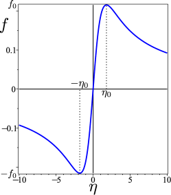
Figure 2: Graph of the odd function $f(\eta)$. It is bounded between $-f_{0}$ and $+f_{0}$, which are the values attained by $f$ at $\eta=\mp\eta_{0}$, respectively. The numerical values are $\eta_{0}\doteq 1.80$ and $f_{0}\doteq 0.22$, which correspond to $u_{0}=-\sqrt{2/3}$ in (72).

The infinitesimal compression ratios computed in (68) serve as sentinels for shock formation.

Remark 8.

By differentiating both sides of (50) and (52) with respect to $\alpha$ and $\beta$, respectively, we obtain that

$$r_{,x}(t,x_{1}(t,\alpha))c_{1}(t,\alpha)=r_{0}^{\prime}(\alpha),\quad\ell_{,x}(t_{0},x_{2}(t,\beta))c_{2}(t,\beta)=\ell_{0}^{\prime}(\beta).$$ (73)

Thus, by Remark 4, if either $r_{0}^{\prime}(\alpha)\neq 0$ or $\ell_{0}^{\prime}(\beta)\neq 0$, then a shock wave is formed in a smooth solution whenever either $c_{1}$ or $c_{2}$ vanishes.

The following Proposition (a more general version of which is stated in [62]) concerns the sign of $c_{1}$ and $c_{2}$.

Proposition 4.

If the pair $(r,\ell)$ is a local solution of class $\mathcal{C}^{1}$ of the system (48) in $[0,t^{\ast})\times\mathbb{R}$, then

$$c_{1}(t,\alpha)>0,\quad c_{2}(t,\beta)>0,\quad\text{for}\ t\in[0,t^{\ast}),\,\text{and every}\ \alpha,\beta\in\mathbb{R}.$$ (74)

Remark 9.

As long as both $r$ and $\ell$ are of class $\mathcal{C}^{1}$, inequalities (74) remain valid, and vice versa, meaning that characteristics in the same family do not crash on one another. If, on the other hand, there exist a value of $\alpha$ and a finite time $t^{\ast}(\alpha)$ or a value of $\beta$ and a finite time $t^{\ast}(\beta)$ such that the corresponding compression ratio vanishes, then by Remark 8 either $r_{,x}$ or $\ell_{,x}$ diverges along the corresponding characteristic, provided that $r_{0}^{\prime}(\alpha)\neq 0$ or $\ell_{0}^{\prime}(\beta)\neq 0$.

Remark 10.

It is proven in [50] (see Theorem 3.4, which builds upon the earlier work [64]) that for all data $r_{0}$ and $\ell_{0}$ with compact support and values ranging in appropriate intervals, system (48) develops a shock wave in a finite time.

Remark 11.

The analysis of hyperbolic systems of two scalar equations in a single spatial variable, such as (48), is much richer in results than the analysis of more general hyperbolic systems. Notable among these are the precise breakdown estimates achieved with Lax’s geometric method [67] (recounted in Theorem 3.5 of [50]). However, they are not generally applicable to our setting, as they would require constraining the data so that $k^{\prime}\neq 0$, which would be rather restrictive an assumption, as by (47) and (48c) this would amount to require that $w_{0}^{\prime}\neq 0$.

Here we build instead on more recent work [62] to establish similar breakdown estimates for more general data. To this end, we collect below a number of preliminary properties of the solutions of (48) that will be instrumental to a detailed analysis of the specific cases we are interested in.

Remark 12.

Every point $(t,x)$ reached by a forward characteristic, so that $x=x_{1}(t,\alpha)$ for some $\alpha\in\mathbb{R}$, can be seen as the end-point at time $t$ of a backward characteristic within the family defined by (51). Such a backward characteristic originates at $\beta=\beta(t,\alpha)$, a point in $\mathbb{R}$ depending on $t$, the time of intersection between the two characteristics, and $\alpha$, the starting point in $\mathbb{R}$ of the forward characteristic (see Fig. 3).

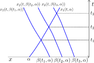
Figure 3: A forward characteristic $x=x_{1}(t,\alpha)$ starting from $\alpha$ at $t=0$ and traversing different time levels, $0<t_{1}<t_{2}<t_{3}$, where it intersects different backward characteristics emanating from $\beta(t_{i},\alpha)$, for $i=1,\,2,\,3$.

Formally, the function $\beta(t,\alpha)$ is implicitly defined by the equation

$$x_{1}(t,\alpha)=x_{2}(t,\beta(t,\alpha).$$ (75a)

Conversely, by exchanging the roles of forward and backward characteristics, we may regard $$\alpha (t,\beta)$$ as a function of defined implicitly by

$$x_{2}(t,\beta)=x_{1}(t,\alpha(t,\beta)).$$ (75b)

Proposition 5.

Equations (75) have a unique solution, $\beta=\beta(t,\alpha)$ and $\alpha=\alpha(t,\beta)$, respectively. The mappings $t\mapsto\beta(t,\alpha)$ and $t\mapsto\alpha(t,\beta)$ are both of class $\mathcal{C}^{1}$, strictly increasing and decreasing, respectively, and such that

$$\beta_{,t}(t,\alpha)=\frac{2k(r_{0}(\alpha)-\ell_{0}(\beta(t,\alpha)))}{c_{2}(t,\beta(t,\alpha))}>0\quad\text{and}\quad\alpha_{,t}(t,\beta)=-\frac{2k(r_{0}(\alpha(t,\beta))-\ell_{0}(\beta))}{c_{1}(t,\alpha(t,\beta))}<0.$$ (76)

Moreover they obey the following bounds,

$$\alpha+\frac{2}{f_{0}||\ell_{0}^{\prime}||_{\infty}}\ln\left(1+f_{0}||\ell_{0}^{\prime}||_{\infty}t\right)\leq\beta(t,\alpha)\leq\alpha+2\delta t\quad\text{and}\quad\beta-2\delta t\leq\alpha(t,\beta)\leq\beta-\frac{2}{f_{0}||r_{0}^{\prime}||_{\infty}}\ln\left(1+f_{0}||r_{0}^{\prime}||_{\infty}t\right),$$ (77)

where $\delta$ is defined in (71) and $f_{0}$ is the maximum of $f$.

Remark 13.

It readily follows from (77) that $\beta(t,\alpha)>\alpha$ and $\alpha(t,\beta)<\beta$, for every $t>0$, and that $\beta(0,\alpha)=\alpha$ and $\alpha(0,\beta)=\beta$.

Definition 3.

According to the geometrical approach adopted here, a shock wave is formed when a characteristic curve becomes degenerate. This occurs when either family becomes infinitely compressive, meaning that there either $c_{1}$ or $c_{2}$ vanishes.

Remark 14.

If a forward characteristic becomes degenerate, then there is $\alpha\in\mathbb{R}$ and a finite time $t^{\ast}(\alpha)$ such that

$$c_{1}(t,\alpha)\to 0\quad\text{as}\quad t\to t^{\ast}(\alpha).$$ (78)

Thus, by (73), $r_{,x}$ must accordingly diverge, provided that $r_{0}^{\prime}(\alpha)\neq 0$, namely

$$r_{,x}(t,x_{1}(t,\alpha))=\frac{r_{0}^{\prime}(\alpha)}{c_{1}(t,\alpha)}\to\operatorname{sgn}(r_{0}^{\prime}(\alpha))\infty\quad\text{as}\quad t\to t^{\ast}(\alpha).$$ (79)

By (41a) and (39), this in turn implies that the second derivatives of $w$ diverge, while the first derivatives develop a discontinuity.

Remark 15.

In a completely parallel way, the degeneracy of a backward characteristic would lead us to identify a critical time $t^{\ast}(\beta)$ where $\ell_{,x}(t,x_{2}(t,\beta))$ would diverge, provided that $\ell_{0}^{\prime}(\beta)\neq 0$. Not to burden our presentation with too many case distinctions, we shall preferentially focus on the possible degeneracy of forward characteristics. When both forward and backward characteristics become degenerate, the actual critical time will be the least between $t^{\ast}(\alpha)$ and $t^{\ast}(\beta)$, for all admissible $\alpha$ and $\beta$ for which these times exist.

In the following section, we shall derive estimates for $t^{\ast}(\alpha)$ and record without explicit proof the corresponding ones for $t^{\ast}(\beta)$.

VI Critical Time Estimates

Here, we build upon the method illustrated in the preceding section to analyze the formation of singularities in the smooth solutions of problem (35) for a broad class of initial data $w_{0}$; we provide an estimate for the critical time $t^{\ast}$ for these singularities to occur, which depends only on $w_{0}$. More particularly, these conditions will be shown to depend only on $r_{0}$: they encompass a large class of initial data.

Theorem 1.

Consider the global Cauchy problem (48) with initial condition $r_{0}(x)=-\ell_{0}(x)\in\mathcal{C}^{1}$ as given in (48c). Assume that $r_{0}$ is bounded and has a finite limit as $x\to+\infty$,

$$\lim_{x\to\infty}r_{0}(x)=:r_{0}(+\infty)\in\mathbb{R}.$$ (80)

If there exists at least one $\alpha\in\mathbb{R}$ such that $r_{0}$ satisfies the condition

$$\operatorname{sgn}\left(r_{0}^{\prime}(\alpha)\left(r_{0}(\alpha)+r_{0}(+\infty)\right)\right)=-1,$$ (81)

then the solution $r(t,x)$ to (48) will develop a singularity along the characteristic curve $x=x_{1}(t,\alpha)$ in a finite time $t^{\ast}(\alpha)$. Similarly, if $r_{0}$ has a finite limit as $x\to-\infty$,

$$\lim_{x\to-\infty}r_{0}(x)=:r_{0}(-\infty)\in\mathbb{R},$$ (82)

and if there exists at least one $\beta\in\mathbb{R}$ such that $r_{0}(x)$ satisfies the condition

$$\operatorname{sgn}\left(r_{0}^{\prime}(\beta)\left(r_{0}(\beta)+r_{0}(-\infty)\right)\right)=+1,$$ (83)

then the solution $\ell(t,x)$ to (48) will develop a singularity along the characteristic curve $x=x_{2}(t,\beta)$ in a finite time $t^{\ast}(\beta)$.

Proof.

We focus on the occurrence of singularities along forward characteristics, which obey (49). By use of Proposition 5, we first estimate $c_{1}(t,\alpha)$ in (68b). Key to this end is to consider the point $(\tau,x_{1}(\tau,\alpha))$ as the endpoint at time $\tau$ of the backward characteristic starting from $\beta(\tau,\alpha)$. Hence, by (52) and (75), we can express (68a) as

$$c_{1}(t,\alpha)=\sqrt{\frac{k(r_{0}(\alpha)-\ell_{0}(\beta(t,\alpha)))}{k(2r_{0}(\alpha))}}g(t,\alpha),$$ (84)

where with the aid of (48c) the function $g$ is defined as

$$g(t,\alpha):=1+r_{0}^{\prime}(\alpha)\sqrt{k(2r_{0}(\alpha))}\int_{0}^{t}f\left(r_{0}(\alpha)+r_{0}(\beta(\tau,\alpha))\right)\operatorname{d}\!\tau.$$ (85)

Thus, for $c_{1}$ to vanish at $t=t^{\ast}(\alpha)$, it must be

$$g(t^{\ast}(\alpha),\alpha)=0.$$ (86)

For $t=0$, $g(0,\alpha)=1$, whereas for $t\to\infty$, the integral in (85) can be easily estimated as $\beta(t,\alpha)$ diverges to $+\infty$ at least logarithmically in consequence of (77). Thus,

$$g(t,\alpha)\approx 1+r_{0}^{\prime}(\alpha)\sqrt{k(2r_{0}(\alpha))}f\left(r_{0}(\alpha)+r_{0}(+\infty)\right)t\quad\text{as}\quad t\to\infty.$$ (87)

This implies that whenever

$$r_{0}^{\prime}(\alpha)f(r_{0}(\alpha)+r_{0}(+\infty))<0,$$ (88)

there always exists a sufficiently large time $t^{\ast}(\alpha)$ such that $g(t^{\ast}(\alpha),\alpha)$ vanishes. Since $\operatorname{sgn}(f(\eta)\eta)=+1$ for all $\eta\neq 0$, (88) is equivalent to (81). ∎

Remark 16.

It follows from (81) and (83) that if $r_{0}(x)$ is even or odd (and correspondingly $r_{0}^{\prime}(x)$ is odd or even), then for a singularity occurring along a forward characteristic originating at $\alpha$, another singularity also occurs along the backward characteristic originating from $\beta=-\alpha$, and $t^{\ast}(\alpha)=t^{\ast}(\beta)$.

An estimate of the critical time $t^{\ast}(\alpha)$ at which the singularity occurs can be provided under more restrictive assumptions on the behavior of $r_{0}(x)$ and $r_{0}^{\prime}(x)$ for $x>\alpha$, with $\alpha$ satisfying (81). We establish these estimates in the following Corollaries.

Corollary 1.

If there exists $\alpha\in\mathbb{R}$ such that, in addition to (81), $r_{0}$ also satisfies

$$\operatorname{sgn}\left(r_{0}^{\prime}(x)r_{0}(\alpha)\right)=-1\quad\text{for every}\quad x\geq\alpha,$$ (89)

then the critical time $t^{\ast}(\alpha)$ can be estimated as

$$t^{\ast}(\alpha)\leq\frac{1}{\sqrt{k(2r_{0}(\alpha))}|r_{0}^{\prime}(\alpha)|\gamma^{+}_{1}(\alpha)}\quad\text{with}\quad\gamma^{+}_{1}(\alpha):=\min\left\{\left|f(2r_{0}(\alpha))\right|,\left|f(r_{0}(\alpha)+r_{0}(+\infty))\right|\right\}.$$ (90)

Proof.

Under the hypothesis on $r_{0}(x)$ stated in Theorem 1, for $\alpha\in\mathbb{R}$ satisfying (81) the forward characteristic $x=x_{1}(t,\alpha)$ becomes infinitely compressive, i.e. (78) holds, after the time $t^{\ast}(\alpha)$ such that $g(t^{\ast}(\alpha),\alpha)=0$, where $g$ is defined as in (85). Since by (77) $\beta(t,\alpha)\geq\alpha$ for every $t\geq 0$, (89) and (76) imply that $r_{0}(\alpha)+r_{0}(\beta(\tau,\alpha))$ is monotonic and keeps the same sign for every $\tau\geq 0$, and so also does $f(r_{0}(\alpha)+r_{0}(\beta(\tau,\alpha)))$: by (81), the asymptotic limit $f(r_{0}(\alpha)+r_{0}(+\infty))$ approached for $\tau\to\infty$ has the same sign as $f(r_{0}(\alpha)+r_{0}(\beta(0,\alpha)))$. Thus,

$$g(t,\alpha) =1-\sqrt{k(2r_{0}(\alpha))}|r_{0}^{\prime}(\alpha)|\int_{0}^{t}|f(r_{0}(\alpha)+r_{0}(\beta(\tau,\alpha)))|\operatorname{d}\!\tau$$

$$\leq 1-\sqrt{k(2r_{0}(\alpha))}|r_{0}^{\prime}(\alpha)|\min\left\{\left|f(2r_{0}(\alpha))\right|,\left|f(r_{0}(\alpha)+r_{0}(+\infty))\right|\right\}t.$$ (91)

Since $g(0,\alpha)=1$, it follows from (91) that $g(t,\alpha)<0$ when the inequality in (90) is violated. This complete the proof of the Corollary. ∎

Remark 17.

A parallel argument applied to backward characteristics proves that if there exists $\beta\in\mathbb{R}$ such that, in addition to (83), $r_{0}$ also satisfies

$$\operatorname{sgn}\left(r_{0}^{\prime}(x)r_{0}(\beta)\right)=+1\quad\text{for every}\quad x\leq\beta,$$ (92)

then the critical time $t^{\ast}(\beta)$ can be estimated as

$$t^{\ast}(\beta)\leq\frac{1}{\sqrt{k(2r_{0}(\beta))}|r_{0}^{\prime}(\beta)|\gamma^{-}_{1}(\beta)}\quad\text{with}\quad\gamma^{-}_{1}(\beta):=\min\left\{\left|f(2r_{0}(\beta))\right|,\left|f(r_{0}(\beta)+r_{0}(-\infty))\right|\right\}.$$ (93)

Corollary 2.

If there exist $\alpha\in\mathbb{R}$ and $\varepsilon>0$, possibly depending on $\alpha$, such that, in addition to (81), $r_{0}$ also satisfies

$$\operatorname{sgn}\left(r_{0}^{\prime}(\alpha)r_{0}(\alpha)\right)=-1,\quad\text{and}\quad|r_{0}(\alpha)+r_{0}(x)|>\varepsilon>0\quad\text{for every}\quad x\geq\alpha,$$ (94)

then

$$t^{\ast}(\alpha)\leq\frac{1}{\sqrt{k[2r_{0}(\alpha)]}|r_{0}^{\prime}(\alpha)|\gamma^{+}_{2}(\alpha)}\quad\text{with}\quad\gamma^{+}_{2}(\alpha):=\min\left\{\left|f\left(\eta\right)\right|:\eta\in[\varepsilon,\sup_{x\geq\alpha}|r_{0}(\alpha)+r_{0}(x)|]\right\}.$$ (95)

Proof.

Unlike the case considered in Corollary 1, here $r_{0}^{\prime}(x)$ can change its sign for $x\geq\alpha$. However, $|r_{0}(\alpha)+r_{0}(\beta(\tau,\alpha))|$ cannot vanish, as it must range between $\varepsilon$ and $\sup_{x\geq\alpha}|r_{0}(\alpha)+r_{0}(x)|$. Accordingly, reasoning as in the proof of Corollary  1, we find that

$$g(t,\alpha)\leq 1-|r_{0}^{\prime}(\alpha)|\sqrt{k(2r_{0}(\alpha))}\min\left\{\left|f\left(\eta\right)\right|:\eta\in[\varepsilon,\sup_{x\geq\alpha}|r_{0}(\alpha)+r_{0}(x)|]\right\}t,$$ (96)

which leads us to (95). ∎

Remark 18.

A similar argument can be applied to the backward characteristics of family (51) to prove that if there exist $\beta\in\mathbb{R}$ and $\varepsilon>0$, possibly depending on $\beta$, such that, in addition to (83), $r_{0}$ also satisfies

$$\operatorname{sgn}\left(r_{0}^{\prime}(\beta)r_{0}(\beta)\right)=+1\quad\text{and}\quad|r_{0}(\beta)+r_{0}(x)|>\varepsilon>0\quad\text{for every}\quad x\leq\beta,$$ (97)

then

$$t^{\ast}(\beta)\leq\frac{1}{\sqrt{k(2r_{0}(\beta))}|r_{0}^{\prime}(\beta)|\gamma^{-}_{2}(\beta)}\quad\text{with}\quad\gamma^{-}_{2}(\beta):=\min\left\{\left|f\left(\eta\right)\right|:\,\eta\in[\varepsilon,\sup_{x\leq\beta}|r_{0}(\beta)+r_{0}(x)|]\right\}.$$ (98)

By minimizing $t^{\ast}(\alpha)$ and $t^{\ast}(\beta)$ among all $\alpha$ and $\beta$ for which a singularity occurs, we can derive an estimate for the singular time $t^{\ast}$ at which a regular solution of system (48) breaks down. In the following Proposition, we collect in a single formal inequality for $t^{\ast}$ the partial estimates in Corollaries 1 and 2 and in Remarks 17 and 18 above.

Proposition 6.

Under the hypotheses of Theorem 1, the critical time $t^{\ast}$ for the existence of a solution of class $\mathcal{C}^{1}$ to system (48) can be estimated as

$$t^{\ast}\leq t_{\mathrm{c}}:=\inf_{\alpha\in\mathbb{R}}\inf_{\gamma(\alpha)}\frac{1}{\sqrt{k(2r_{0}(\alpha))}|r_{0}^{\prime}(\alpha)|\gamma(\alpha)},$$ (99)

where

$$\gamma(\alpha):=\begin{cases}\min\{|f(2r_{0}(\alpha))|,|f(r_{0}(\alpha)+r_{0}(+\infty))|\}&if\ \operatorname{sgn}(r_{0}^{\prime}(x)r_{0}(\alpha))=-1\ \forall\ x\geq\alpha,\\ \min\{|f(2r_{0}(\alpha))|,|f(r_{0}(\alpha)+r_{0}(-\infty))|\}&if\ \operatorname{sgn}(r_{0}^{\prime}(x)r_{0}(\alpha))=+1\ \forall\ x\leq\alpha,\\ \min\{|f(\eta)|:\eta\in[\varepsilon,\sup_{x\leq\alpha}|r_{0}(\alpha)+r_{0}(x)|]\}&if\ \operatorname{sgn}(r_{0}^{\prime}(\alpha)r_{0}(\alpha))=+1\ \text{\emph{and}}\ |r_{0}(\alpha)+r_{0}(x)|>\varepsilon>0\ \forall\ x\geq\alpha,\\ \min\{|f(\eta)|:\eta\in[\varepsilon,\sup_{x\leq\alpha}|r_{0}(\alpha)+r_{0}(x)|]\}&if\ \operatorname{sgn}(r_{0}^{\prime}(\alpha)r_{0}(\alpha))=-1\ \text{\emph{and}}\ |r_{0}(\alpha)+r_{0}(x)|>\varepsilon>0\ \forall\ x\leq\alpha,\\ 0&\text{\emph{otherwise}}.\end{cases}$$ (100)

Remark 19.

When $\gamma(\alpha)=0$, we conventionally set equal to $+\infty$ the argument of the double $\inf$ on the right-hand side of (99).

Remark 20.

By (80) and (82), $\gamma(\alpha)>0$, at least for $\alpha\to+\infty$ or $\alpha\to-\infty$. Thus, the upper estimate $t_{\mathrm{c}}$ for $t^{\ast}$ in (99) is never $+\infty$ and a finite critical time always exist at which a regular solution of (48) breaks down.

In the following section, we shall see a number of applications of our method where the estimate (99), despite its complicated appearance, is proven effective and delivers critical times very close to those calculated numerically.

VII Applications

As illustrative examples, we consider initial profiles $w_{0}$ for the twist angle that exhibit a strong concentration of distortion around $x=0$, which fades away at infinity without ever vanishing. Thus, by (28), the more distorted core propagates faster than the distant tails, possibly overtaking them: intuitively, this should prompt the creation of a singularity in a finite time. We shall see here how such an intuitive prediction is indeed confirmed by the estimate (99).

Specifically, we shall consider two types of initial profiles $w_{0}$, namely, a kink and a bump. In either cases, we shall both estimate the critical time $t^{\ast}$ and identify the characteristics along which a singularity first occurs.

Numerical solutions of the global Cauchy problem (35) will also be provided: they are shown to be in good agreement with the theoretical predictions.

VII.1 Kink

We consider the following initial twist profile

$$w_{0}(\kappa,\zeta;x):=-\frac{2\kappa}{\pi}\arctan\frac{x}{\zeta},$$ (101)

where $\kappa$ and $\zeta$ are positive parameters. This is a kink representing a smooth transition of the twist angle between two asymptotic values depending on $\kappa$, in an effective width around the origin depending on $\zeta$. Fig. 4 illustrates the graphs of the initial profile $w_{0}$ in (101) for different values of $\zeta$ and $\kappa$: either increasing $\zeta$ or decreasing $\kappa$ makes the initial profile less distorted (whereas either decreasing $\zeta$ or increasing $\kappa$ makes the initial profile more distorted).

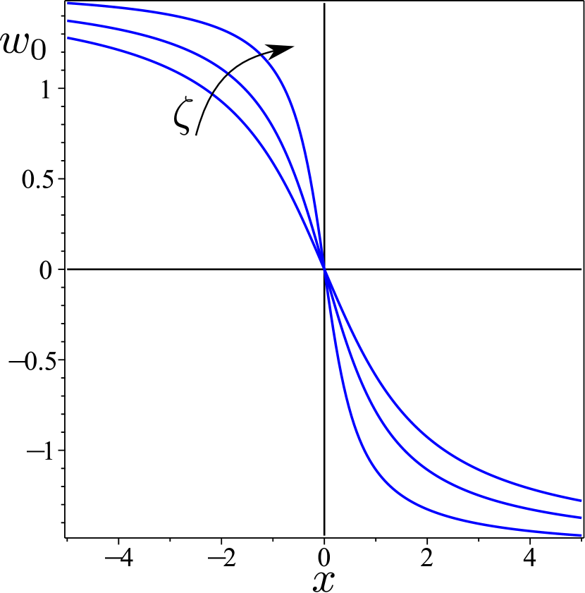
(a) $\kappa=\pi/2$, $\zeta=1/2,\,1,\,3/2$.

(b) $\zeta=1/2$, $\kappa=\pi/4,\,\pi/2,\,3\pi/2$.

Figure 4: Initial profile of the twist angle $w_{0}$ represented by (101) for several values of the parameters $\kappa$ and $\zeta$, which describe the amplitude and width of the kink, respectively.

By (48c) and (44), $r_{0}$ is given by

$$r_{0}(\kappa,\zeta;x)=\frac{1}{2}\left(\xi\sqrt{1+\xi^{2}}+\hbox{arcsinh}\,\xi\right),\quad\,\hbox{where}\quad\xi:=\frac{2\kappa\zeta}{x^{2}+\zeta^{2}}.$$ (102)

The graph of $r_{0}$ is illustrated in Fig. 5 for different values of $\kappa$ and $\zeta$. Since $r_{0}$ is an even function, by Theorem 1, we need only forward characteristics: if a singularity arises along a forward characteristic originating at $\alpha$, a singularity will also occur at the same critical time along the (symmetric) backward characteristic originating at $\beta=-\alpha$.

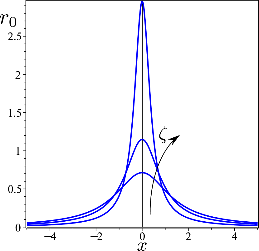
(a) $\kappa=\pi/2$, $\zeta=1/2,\,1,\,3/2$.

(b) $\zeta=1/2$, $\kappa=\pi/4,\,\pi/2,\,3\pi/2$.

Figure 5: Initial profile of the Riemann invariant $r_{0}$ in (102) corresponding to the initial twist $w_{0}$ illustrated in Fig. 4.

Here, $r_{0}(+\infty)=0$ and condition (81) is satisfied for every $\alpha>0$. Consequently, a singularity occurs in a finite time for each of these values. Thus, the upper estimate $t_{\mathrm{c}}$ for the critical time $t^{\ast}$ in (99) reduces to

$$t_{\mathrm{c}}=\inf_{\alpha>0}\frac{1}{\sqrt{k[2r_{0}(\alpha)]}|r_{0}^{\prime}(\alpha)|\gamma(\alpha)}\quad\text{with}\quad\gamma(\alpha)=\min\left\{f(2r_{0}(\alpha)),f(r_{0}(\alpha))\right\}.$$ (103)

Fig. 6 shows how $t_{\mathrm{c}}$ in (103) depends on both $\kappa$ and $\zeta$: it decreases with $\kappa$ and increases with $\zeta$. This behavior is in accord with intuition: as $\kappa$ decreases or $\zeta$ increases, the initial profile becomes more spread out and less prominent, suggesting that the kink’s core propagates more slowly, thus delaying the shock formation.

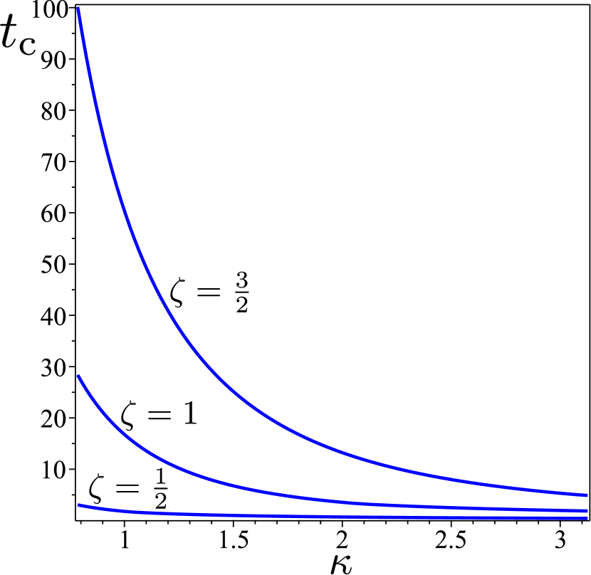
(a) $\kappa\in[\pi/4,3\pi/2]$, $\zeta=1/2,\,1,\,3/2$.

(b) $\zeta\in[1/2,3/2]$, $\kappa=\pi/4,\,\pi/2,\,3\pi/2$.

Figure 6: The time $t_{\mathrm{c}}$ is the upper estimate in (103) for the critical time $t^{\ast}$ of a regular solution of the global Cauchy problem (35) with initial profile (101). In particular, for $\kappa=\pi/2$ and $\zeta=1/2$, $t_{\mathrm{c}}\doteq 0.9$.

Numerical solutions of the Cauchy problem (35) closely corroborate our theoretical predictions. We present here the case where in (101) $\kappa=\pi/2$ and $\zeta=1/2$. The initial profile generates two symmetric waves propagating in opposite directions. We computed the conserved quantities $M$ and $E$ introduced in Propositions 1 and 2, respectively, and used them to monitor the accuracy of our numerical solutions. Our calculations indicate the existence of a critical time, estimated as $t^{\ast}\doteq 0.8$, at which the solution exhibits a singularity. Fig. 7 illustrates a typical numerical solution $w(t,x)$ and its spatial derivatives $w_{,x}(t,x)$ and $w_{,xx}(t,x)$ for a sequence of times $t$ in the interval $[0,t^{\ast})$. A snapshot at $t=t^{\ast}$ is shown in Fig. 8(a). The observed behavior is in good agreement with our theory: a shock is formed in a finite time, at which $w_{,x}$ becomes discontinuous, and second derivatives diverge.

The critical time identified numerically agrees with our theoretical upper estimate $t_{\mathrm{c}}\doteq 0.9$. The infimum in (99) is correspondingly attained for $\alpha\doteq 0.26$. Figure 8(b) shows a set of forward characteristics determined numerically: they all start from points around $\alpha=0.26$ and become infinitesimally compressive (i.e., with $c_{1}=0$) in a finite time: the one that becomes so before the others (at $t=t^{\ast}$) starts at $\alpha\doteq 0.27$, again in good agreement with theory.

(a) $t=0.15$.

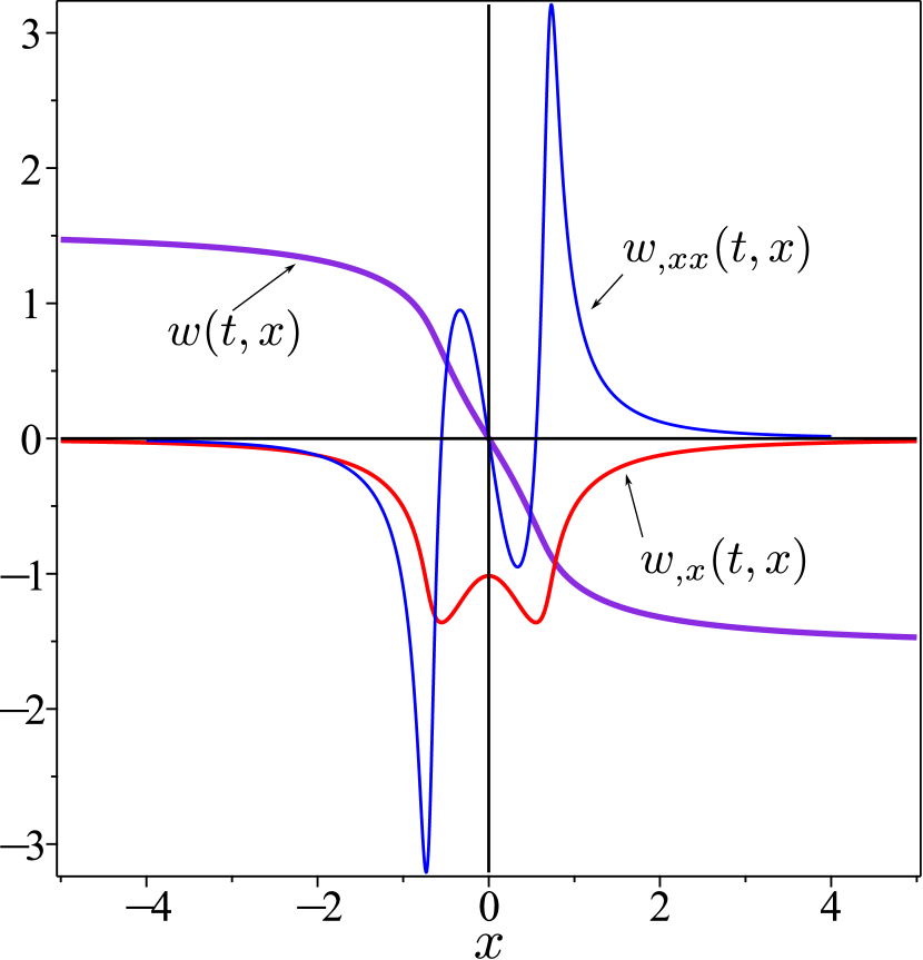
(b) $t=0.3$.

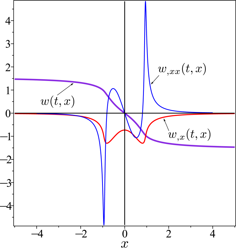
(c) $t=0.45$.

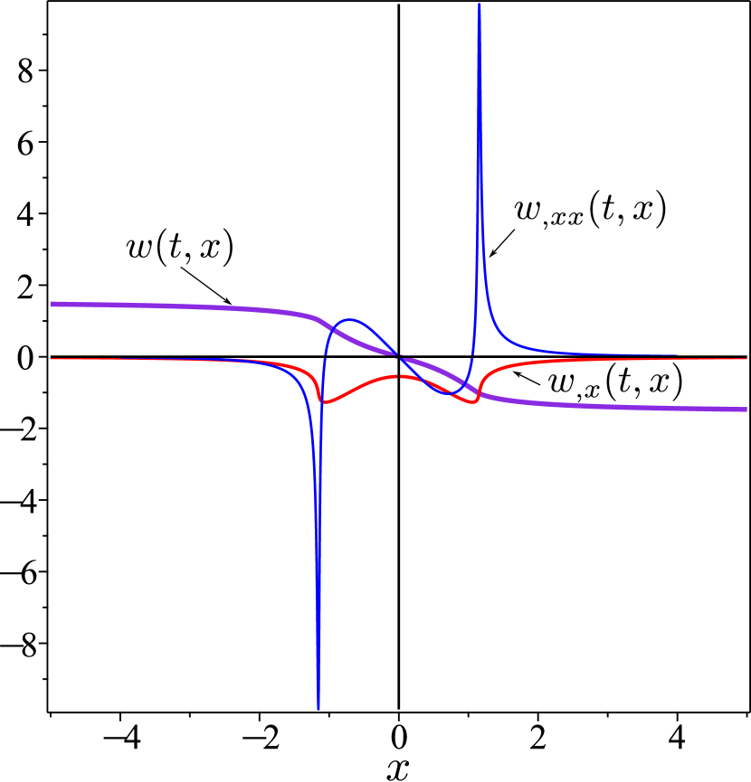
(d) $t=0.6$.

Figure 7: Graphs of the numerical solution $w(t,x)$ and its spatial derivatives $w_{,x}(t,x)$ and $w_{,xx}(t,x)$ for the initial profile $w_{0}$ in (101) with $\kappa=\pi/2$, $\zeta=1/2$. The time sequence suggests that $w_{,xx}$ tends to develop two antisymmetric spikes, whereas $w_{,x}$ tends to develop symmetric jumps.

(a) Graphs of the numerical solution $w(t^{\ast},x)$ and its spatial derivatives $w_{,x}(t^{\ast},x)$ and $w_{,xx}(t^{\ast},x)$ at the critical time $t^{\ast}\doteq 0.8$.

(b) Forward characteristic curves originating at different values of $\alpha>0$, each developing a singularity in a finite time. The one starting at $\alpha\doteq 0.27$ (marked in red) becomes infinitely compressive (that is, $c_{1}=0$) before all others.

Figure 8: Singularity emerging at the critical time $t^{\ast}\doteq 0.8$ along the solution of (35) with initial profile (101) for $\kappa=\pi/2$, and $\zeta=1/2$.

VII.2 Bump

We next consider a Gaussian profile for the initial twist angle $w_{0}$, which represents a localized bump in a otherwise nearly uniform director field,

$$w_{0}(\kappa,\zeta;x):=\kappa\mathrm{e}^{-\frac{x^{2}}{2\zeta^{2}}}.$$ (104)

Here, the amplitude $\kappa$ and the variance $\zeta$ are positive parameters that control the height of the bump and its width, respectively. Fig. 9 illustrates how upon increasing $\zeta$ (or decreasing $\kappa$), the initial distortion becomes less pronounced (and the ensuing smooth solution of (35) presumably longer lived).

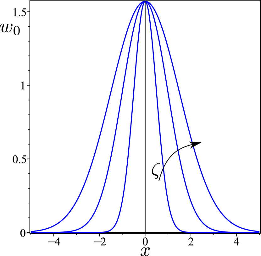
(a) $\kappa=\pi/2$, $\zeta=1/2,\,1,\,3/2$.

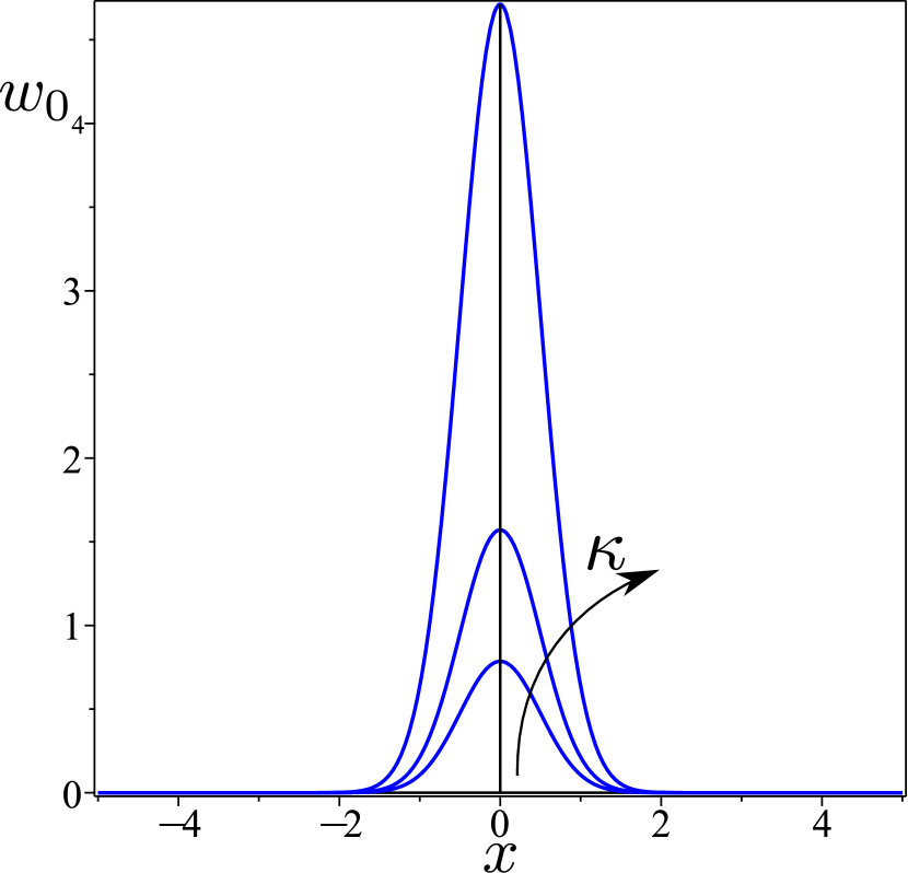
(b) $\zeta=1/2$, $\kappa=\pi/4,\,\pi/2,\,3\pi/2$.

Figure 9: Initial profile of the twist angle $w_{0}$ represented by (104) for several values of the parameters $\kappa$ and $\zeta$, which describe the aplitude and width of the bump, respectively.

By (48c) and (44), $r_{0}$ is given by

$$r_{0}(\kappa,\zeta;x)=\frac{1}{2}\left(\xi\sqrt{1+\xi^{2}}+\hbox{arcsinh}\,\xi\right),\quad\text{where}\quad\xi:=-\frac{x}{\zeta^{2}}w_{0}(x,\kappa,\zeta)=-\frac{\kappa}{\zeta^{2}}x\mathrm{e}^{-\frac{x^{2}}{2\zeta^{2}}}$$ (105)

and its graph is illustrated in Fig. 10 for different values of $\kappa$ and $\zeta$. As $r_{0}$ is an odd function, by Theorem 1, it suffices to look for the occurrence of singularities along the forward characteristics.

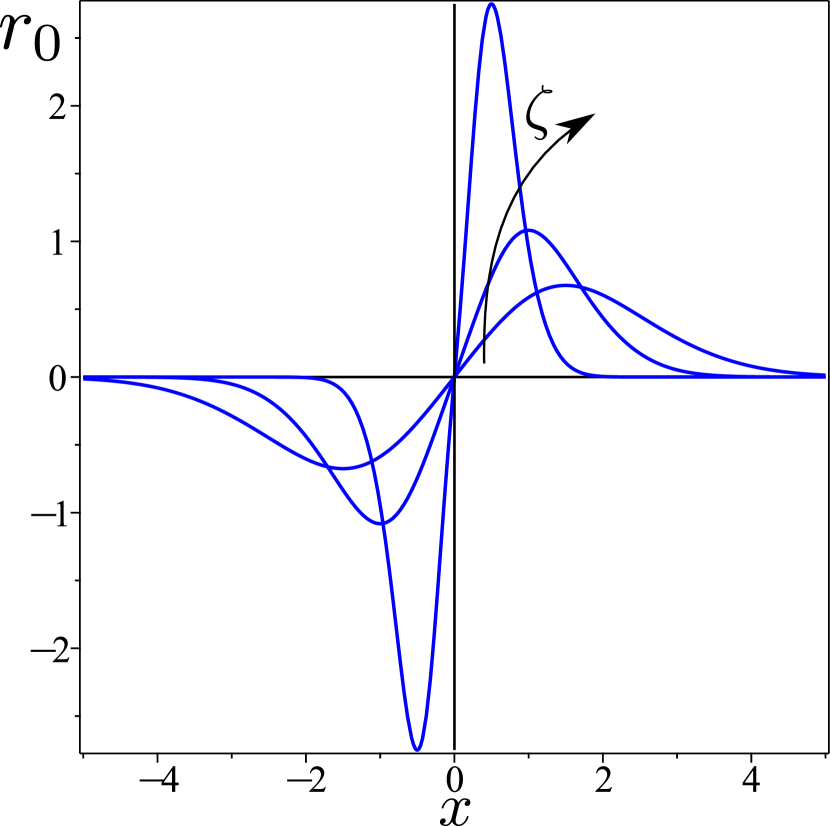
(a) $\kappa=\pi/2$, $\zeta=1/2,\,1,\,3/2$.

(b) $\zeta=1/2$, $\kappa=\pi/4,\,\pi/2,\,3\pi/2$.

Figure 10: Initial profile of the Riemann invariant $r_{0}$ in (105) corresponding to the initial twist $w_{0}$ illustrated in Fig. 9.

Since $r_{0}(+\infty)=0$, the values of $\alpha\in\mathbb{R}$ for which $r_{0}$ satisfies condition (81) can be found for both $\alpha\in(-\zeta,0)$ and $\alpha>\zeta$. Singularities develop in a finite time along every characteristic starting from these values of $\alpha$, but only for $\alpha>\zeta$ is $t_{\mathrm{c}}$ in (99) finite.

Fig. 11 illustrates how $t_{\mathrm{c}}$ depends on both $\kappa$ and $\zeta$; as expected, $t_{\mathrm{c}}$ decreases upon increasing $\kappa$ or decreasing $\zeta$, both actions corresponding to an enhancement of distortion in the initial twist profile.

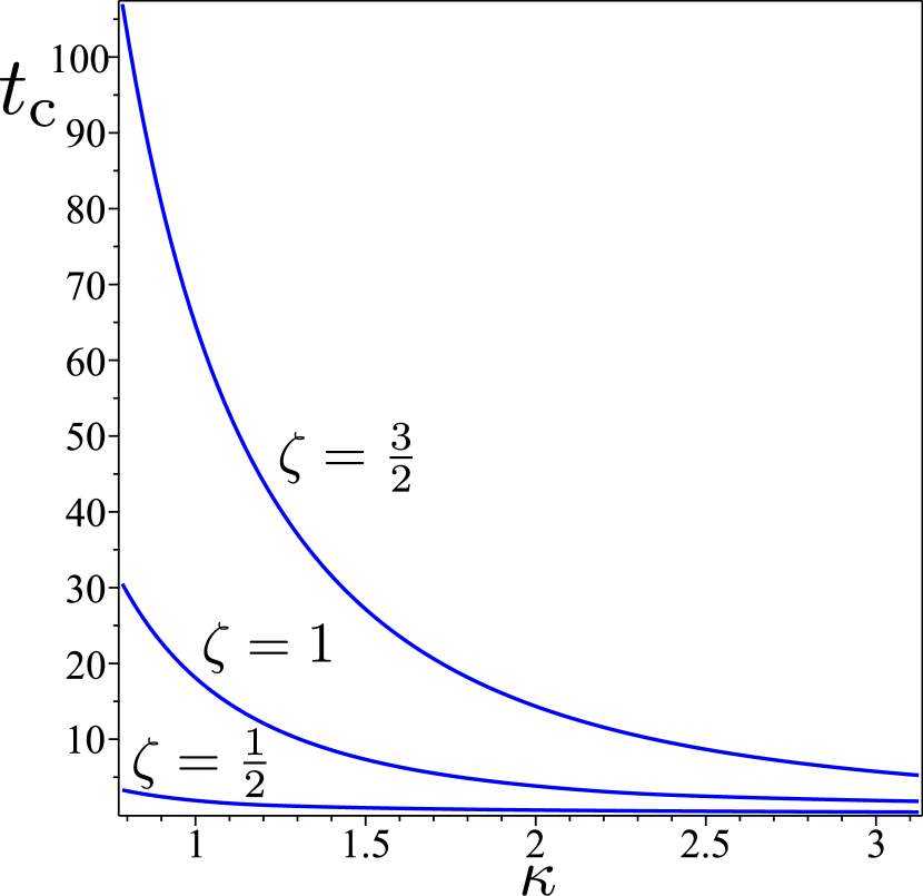
(a) $\kappa\in[\pi/4,3\pi/2]$, $\zeta=1/2,\,1,\,3/2$.

(b) $\zeta\in[1/2,3/2]$, $\kappa=\pi/4,\,\pi/2,\,3\pi/2$.

Figure 11: The time $t_{\mathrm{c}}$ delivered by (99) is the upper estimate of the critical time $t^{\ast}$ of a regular solution of the global Cauchy problem (35), with initial profile (104). In particular, for $\kappa=\pi/2$ and $\zeta=1/2$, $t_{\mathrm{c}}\doteq 0.9$.

Numerical solutions of the global Cauchy problem (35) with initial profile (104) confirm our theoretical predictions. Specifically, for $\kappa=\pi/2$ and $\zeta=1/2$, Fig. 12 depicts $w(t,x)$ and its spatial derivatives $w_{,x}(t,x)$ and $w_{,xx}(t,x)$ for times in the interval $[0,t^{\ast})$, with $t^{\ast}\doteq 0.8$.

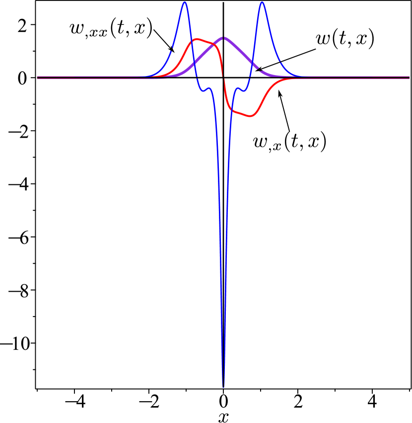
(a) $t=0.15$.

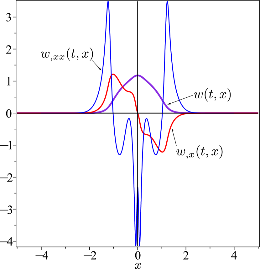
(b) $t=0.3$.

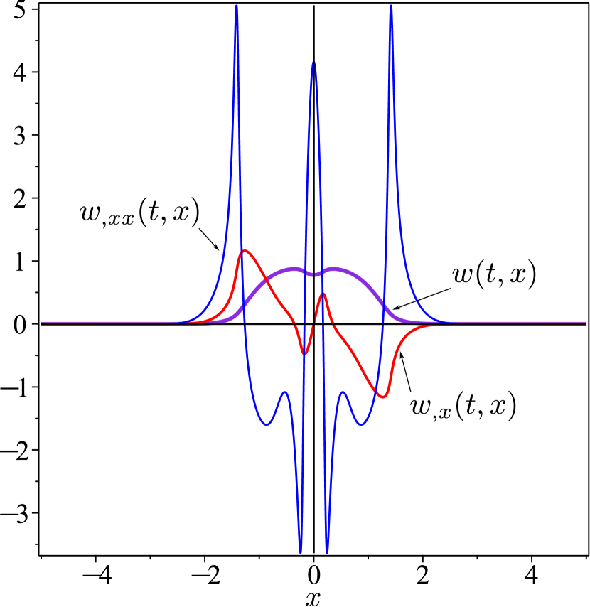
(c) $t=0.45$.

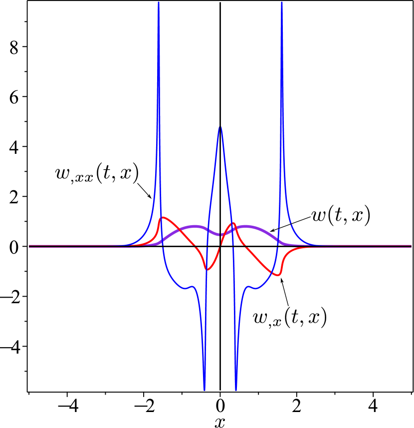
(d) $t=0.6$.

Figure 12: Graphs of the numerical solution $w(t,x)$ and its spatial derivatives $w_{,x}(t,x)$ and $w_{,xx}(t,x)$ for the initial profile in (104) with $\kappa=\pi/2$, $\zeta=1/2$. The time sequence suggests that $w_{,xx}$ tends to develop two symmetric spikes, whereas $w_{,x}$ tends to develop antisymmetric jumps.

The graphs at time $t=t^{\ast}$ are illustrated in Fig. 13(a). Our numerical results indicate that a singularity occurs along forward characteristics originating at $\alpha\doteq-0.4$ and $\alpha\doteq 0.75$, which become infinitesimally compressive (that is, with $c_{1}=0$) at approximately the same time $t\approx t^{\ast}$, within our numerical accuracy (see Fig. 13(b)). These findings agree well with our theory, as (99) delivers $t_{\mathrm{c}}\doteq 0.9$, with the infimum actually attained at $\alpha\doteq 0.78$.

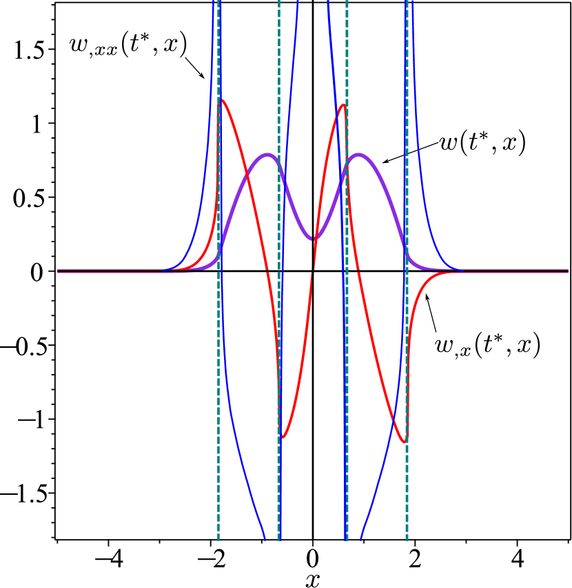
(a) Graphs of the numerical solution $w(t^{\ast},x)$ and its spatial derivatives $w_{,x}(t^{\ast},x)$ and $w_{,xx}(t^{\ast},x)$ at the critical time $t^{\ast}\doteq 0.8$.

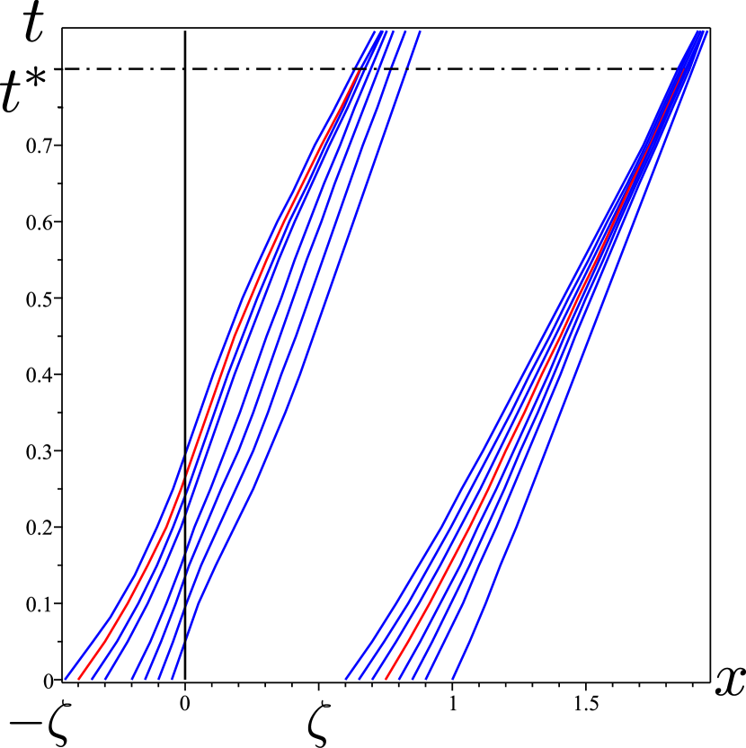
(b) Forward characteristic curves originating at different values of $\alpha\in(-\zeta,0)$ and $\alpha>\zeta$, each developing a singularity in a finite time. The ones starting at $\alpha\doteq-0.4$ and $\alpha\doteq 0.75$ become infinitesimally compressive (that is, $c_{1}=0$) at approximately the same time, $t\approx t^{\ast}$, before all others.

Figure 13: Singularity emerging at the critical time $t^{\ast}\doteq 0.8$ along the solution of (35) for the initial profile (104) with $\kappa=\pi/2$, $\zeta=1/2$.

VIII Conclusions

It has long been known in liquid crystal science that for quadratic elastic energy densities (such as that delivered by the classical Frank-Oseen formula), all weak twist shock waves decay in a finite time, and so they are physically irrelevant. If, on the contrary, the elastic energy density grows more than quadratically in the twist measure, weaker twist shock waves (bearing discontinuities in derivatives of order higher than two) decay rapidly, whereas acceleration shock waves persist and can even evolve in ordinary shock waves (bearing discontinuities in the first derivatives).

This may just appear as a mere mathematical curiosity, as no firm physical ground is available to justify an energy density more than quadratic in the measure of twist for ordinary liquid crystals. The picture changes, however, when one considers chromonic phases, for which a number of studies (both theoretical and experimental) have suggested that a quartic twist energy may be plausible.

For these materials, shock waves may thus result from the evolution of accelartion waves. One may also say that strong shock waves are the only ones eventually surviving. The quest of this paper went the opposite way. We asked whether a shock wave could arise in a finite time from a smooth solution of the (non-linear) wave equation associated with a quartic twist energy. Answering generically for the positive this question would identify shock waves as attractors in the propagation of twist waves in chromonics.

We considered the global Cauchy problem with zero initial velocity, for which we identified (in Theorem 1) mild assumptions on the initial distortion profile that guarantee that the ensuing smooth solution breaks down in a finite time $t^{\ast}$, giving way to the formation of a shock. Whenever these hypotheses are satisfied, an upper estimate for the critical time $t^{\ast}$ can be given (see Proposition 6), which numerical calculations performed in a number of exemplary cases confirmed to be rather accurate.

In particular, we proved that under the assumptions of Theorem 1 all initial profiles break down in a finite time. This conclusion is somehow reminiscent of the result of the classical theory for hyperbolic equations stating that (under appropriate assumptions) initial profiles with compact support always break down in a finite time. However, this is just a superficial similarity, as the assumptions of the classical theory do not apply to our case, and our analysis was built on much more recent results.

The generic breaking of smooth twist waves in chromonic liquid crystals that this paper has highlighted (at least in the vicinity of their nematic-to-isotropic transition) may become a possible experimental signature of the validity of the elastic quartic twist theory adopted here.

We have confined attention to the conservative wave equation, which can be justified on physical grounds only when chromonics are in the vicinity of their isotropic phase. The dissipative case is more realistic, but far more difficult: one relevant issue would be whether dissipation could prevent the formation of a shock or not. Most of the mathematical methodology applied in this paper would not be directly applicable to the dissipative case. In the near future we plan to address this issue by developing appropriate mathematical tools.

Appendix A Governing Equations

Our aim here is to derive equations (25), (24) and (23) from (1a) and (1b) when $W=W_{\mathrm{QT}}$ as in (15) and $\bm{n}$ is represented as in (21).

First, it easily follows from (21) that

$$\nabla\bm{n}=w_{,x}\bm{n}_{\perp}\otimes\bm{e}_{x},$$ (106)

where $\bm{n}_{\perp}:=\bm{e}_{x}\times\bm{n}$. The equations in (22) follow immediately from (106).

Second, we remark that derivatives such as $\frac{\partial W}{\partial\nabla\bm{n}}$, $\frac{\partial R}{\partial\mathbf{D}}$, and $\frac{\partial R}{\partial\mathring{\bm{n}}}$ are to be interpreted in the intrinsic sense (as explained, for example, in [68, p. 133]). Thus, the first is a tensor whose transpose annihilates $\bm{n}$, the second is a traceless, symmetric tensor, and the third is a vector orthogonal to $\bm{n}$. In particular, since

$$\frac{\partial T}{\partial\nabla\bm{n}}=\mathbf{W}(\bm{n}),$$ (107)

where $\mathbf{W}(\bm{n})$ is the skew-symmetric tensor associated with $\bm{n}$, by (22) and (15), we obtain from (18) that the Cauchy stress tensor $\mathbf{T}$ can be written as

$$\mathbf{T}=-p\bm{\mathrm{I}}-K_{22}w_{,x}^{2}\left(1+a^{2}w_{,x}^{2}\right)\bm{e}_{x}\otimes\bm{e}_{x}+w_{,t}(\mu_{2}\bm{n}_{\perp}\otimes\bm{n}+\mu_{3}\bm{n}\otimes\bm{n}_{\perp}),$$ (108)

which follows from

$$\frac{\partial W_{\mathrm{QT}}}{\partial\nabla\bm{n}}=-K_{22}w_{,x}^{2}(1+a^{2}w_{,x}^{2})\mathbf{W}(\bm{n}),$$ (109)

once use has also been made of the identities

$$\frac{1}{2}\frac{\partial}{\partial\nabla\bm{n}}\operatorname{tr}(\nabla\bm{n})^{2}=\mathbf{P}(\bm{n})(\nabla\bm{n})^{\mathsf{T}}\quad\text{and}\quad\partial_{t}\bm{n}=w_{,t}\bm{n}_{\perp},$$ (110)

where $\mathbf{P}(\bm{n}):=\mathbf{I}-\bm{n}\otimes\bm{n}$ is the projector onto the plane orthogonal to $\bm{n}$. Furthermore, since (21) implies that

$$\operatorname{div}\bm{n}=\operatorname{div}\bm{n}_{\perp}=0\quad\text{and}\quad(\nabla\bm{n})\bm{n}_{\perp}=(\nabla\bm{n}_{\perp})\bm{n}=\bm{0},$$ (111)

equation (25) follows at once from (20a) upon computing $\operatorname{div}\mathbf{T}$ from (108).

Similarly, since in general

$$\frac{\partial T}{\partial\bm{n}}=\mathbf{P}(\bm{n})\operatorname{curl}\bm{n},$$ (112)

use of (106) leads us to

$$\frac{\partial W_{\mathrm{QT}}}{\partial\bm{n}}=\bm{0},$$ (113)

whenever $\bm{n}$ is as in (21). Moreover, since

$$\operatorname{div}\mathbf{W}(\bm{n})=-\operatorname{curl}\bm{n}=w_{,x}\bm{n},$$ (114)

where the second equation requires (106), we can write the balance equation (1b) in the explicit form

$$\sigma(w_{,tt}\bm{n}_{\perp}-w_{,t}^{2}\bm{n})+\gamma_{1}w_{,t}\bm{n}_{\perp}+K_{22}\left[w_{,x}^{2}\left(1+a^{2}w_{,x}^{2}\right)\bm{n}-w_{,xx}\left(1+3a^{2}w_{,x}^{2}\right)\bm{n}_{\perp}\right]=\mu\bm{n}.$$ (115)

Equations (24) and (23) in the main text then follow by projecting (115) along $\bm{n}$ and $\bm{n}_{\perp}$, respectively.

Appendix B Proof of Auxiliary Results

In this Appendix, we present for completeness the proofs of two Propositions stated in the main text.

Proof of Proposition 3.

We differentiate both sides of the first equation in (49) with respect to $\alpha$, and we find that

$$\frac{\partial}{\partial\alpha}\left(\frac{\operatorname{d}\!x_{1}}{\operatorname{d}\!t}(t,\alpha)\right)=\frac{\partial}{\partial\alpha}k\left(r_{0}(\alpha)-\ell(t,x_{1}(t,\alpha))\right)=k^{\prime}\left(r_{0}(\alpha)-\ell(t,x_{1}(t,\alpha))\right)\left(r_{0}^{\prime}(\alpha)-\ell_{,x}(t,x_{1}(t,\alpha))\frac{\partial x_{1}}{\partial\alpha}(t,\alpha)\right).$$ (116)

We now derive an alternative expression for $\ell_{,x}(t,x_{1}(t,\alpha))$: by (48b) and (49) we obtain that

$$\frac{\operatorname{d}\!}{\operatorname{d}\!t}\ell(t,x_{1}(t,\alpha))=\ell_{,t}(t,x_{1}(t,\alpha))+\ell_{,x}(t,x_{1}(t,\alpha))\frac{\operatorname{d}\!x_{1}}{\operatorname{d}\!t}(t,\alpha)=2k\left(r_{0}(\alpha)-\ell(t,x_{1}(t,\alpha))\right)\ell_{,x}(t,x_{1}(t,\alpha)),$$ (117)

from which it follows that

$$\ell_{,x}(t,x_{1}(t,\alpha))=\frac{1}{2k\left(r_{0}(\alpha)-\ell(t,x_{1}(t,\alpha))\right)}\frac{\operatorname{d}\!}{\operatorname{d}\!t}\ell(t,x_{1}(t,\alpha)).$$ (118)

Letting

$$H(\eta):=\int_{0}^{\eta}\frac{k^{\prime}(y)}{2k(y)}\operatorname{d}\!y=\frac{1}{2}\ln k(\eta),$$ (119)

where also (47) has been used, with the aid of (118) we arrive at

$$-k^{\prime}\left(r_{0}(\alpha)-\ell(t,x_{1}(t,\alpha))\right)\ell_{,x}(t,x_{1}(t,\alpha))=\frac{\operatorname{d}\!H}{\operatorname{d}\!t}(r_{0}(\alpha)-\ell(t,x_{1}(t,\alpha)))$$ (120)

because

$$\frac{\operatorname{d}\!}{\operatorname{d}\!t}H\left(r_{0}(\alpha)-\ell(t,x_{1}(t,\alpha))\right)=-\frac{k^{\prime}\left(r_{0}(\alpha)-\ell(t,x_{1}(t,\alpha))\right)}{2k\left(r_{0}(\alpha)-\ell(t,x_{1}(t,\alpha))\right)}\frac{\operatorname{d}\!}{\operatorname{d}\!t}\ell(t,x_{1}(t,\alpha)).$$ (121)

Then, (116) reduces to

$$\frac{\operatorname{d}\!}{\operatorname{d}\!t}c_{1}(t,\alpha)=k^{\prime}\left(r_{0}(\alpha)-\ell(t,x_{1}(t,\alpha))\right)r_{0}^{\prime}(\alpha)+\frac{\operatorname{d}\!}{\operatorname{d}\!t}H\left(r_{0}(\alpha)-\ell(t,x_{1}(t,\alpha))\right)c_{1}(t,\alpha).$$ (122)

This is an ODE in the general form

$$\dot{c}_{1}-\dot{h}_{1}c_{1}=h,$$ (123)

where

$$h_{1}(t,\alpha):=H\left(r_{0}(\alpha)-\ell(t,x_{1}(t,\alpha))\right)\quad\text{and}\quad h(t,\alpha):=k^{\prime}\left(r_{0}(\alpha)-\ell(t,x_{1}(t,\alpha))\right)r_{0}^{\prime}(\alpha).$$ (124)

By letting $A(t,\alpha):=h_{1}(t,\alpha)-h_{1}(0,\alpha)$, we obtain the following solution of (123),

$$c_{1}(t,\alpha)=\mathrm{e}^{A(t,\alpha)}\left[c_{1}(0,\alpha)+\int_{0}^{t}f(\tau)\mathrm{e}^{-A(\tau,\alpha)}\operatorname{d}\!\tau\right],$$ (125)

and so

$$c_{1}(t,\alpha)=\mathrm{e}^{h_{1}(t,\alpha)-h_{1}(0,\alpha)}\left\{1+r_{0}^{\prime}(\alpha)\int_{0}^{t}k^{\prime}\left(r_{0}(\alpha)-\ell(\tau,x_{1}(\tau,\alpha))\right)\mathrm{e}^{h_{1}(0,\alpha)-h_{1}(\tau,\alpha)}\operatorname{d}\!\tau\right\},$$ (126)

where, by (124) and (48c), $h_{1}(0,\alpha)=H(r_{0}(\alpha)-\ell_{0}(\alpha))=H(2r_{0}(\alpha))$, while $c_{1}(0,\alpha)=1$.

We can show in the same way that

$$c_{2}(t,\beta)=\mathrm{e}^{h_{2}(t,\beta)-h_{2}(0,\beta)}\left\{1+\ell_{0}^{\prime}(\beta)\int_{0}^{t}k^{\prime}\left(r_{0}(\tau,x_{2}(\tau,\beta))-\ell_{0}(\beta)\right)\mathrm{e}^{h_{2}(0,\beta)-h_{2}(\tau,\beta)}\operatorname{d}\!\tau\right\}.$$ (127)

Here $h_{2}(t,\beta):=H\left(r(t,x_{2}(t,\beta))-\ell_{0}(\beta)\right)$, and so $h_{2}(0,\beta)=H(2r_{0}(\beta))$, where (48c) has also been used.

Finally, we can write

$$\mathrm{e}^{h_{1}(t,\alpha)-h_{1}(0,\alpha)}=\sqrt{\frac{k(r_{0}(\alpha)-\ell(t,x_{1}(t,\alpha)))}{k(2r_{0}(\alpha))}}\quad\text{and}\quad\mathrm{e}^{h_{2}(t,\beta)-h_{2}(0,\beta)}=\sqrt{\frac{k(r(t,x_{2}(t,\beta))-\ell_{0}(\beta))}{k(2r_{0}(\beta))}}.$$ (128)

thus obtaining equations (68) in the main text. ∎

Proof of Proposition 5.

The existence of the unique solution $\beta=\beta(t,\alpha)$ is a consequence of the fact that for any $\tau\in[0,t)$ the Cauchy problem

$$\begin{cases}\frac{\operatorname{d}\!y_{2}}{\operatorname{d}\!\tau}(\tau,t,\alpha)=-k(\tau,y_{2}(\tau,t,\alpha)),\\ y_{2}(t,t,\alpha)=x_{1}(t,\alpha),\end{cases}$$ (129)

has a unique solution $y_{2}(\tau,t,\alpha)$ for $\tau\in[0,t^{\ast})$. We define $\beta(t,\alpha):=y_{2}(0,t,\alpha)$ and $y_{2}(\tau,t,\alpha)=x_{2}(\tau,\beta(t,\alpha))$, where $x_{2}$ is solution of (51). Thus, $\beta(t,\alpha)$ represents the point from which the backward characteristic $x_{2}$ starts. By (51), we conclude that $\beta(t,\alpha)>\alpha$ for every $t\in(0,t^{\ast})$, and $\beta(0,\alpha)=\alpha$.

By differentiating both sides of (75a) with respect to $t$, and using (49) and (51), we obtain (76).

Next, by integrating both sides of (49) with respect to $t$ and using (71), we arrive at

$$x_{1}(t,\alpha)=\alpha+\int_{0}^{t}k(r(\alpha)-\ell(\tau,x_{1}(\tau,\alpha)))\operatorname{d}\!\tau\leq \alpha+\delta t,$$ (130a)

$$x_{2}(t,\beta(t,\alpha))=\beta(t,\alpha)-\int_{0}^{t}k(r(\tau,x_{2}(\tau,\beta(t,\alpha)))-\ell_{0}(\beta(t,\alpha)))\operatorname{d}\!\tau\geq \beta(t,\alpha)-\delta t.$$ (130b)

By (75a) and (130a), (130b) gives that

$$\beta(t,\alpha)\leq\alpha+2\delta t.$$ (131)

To establish a lower bound for $\beta(t,\alpha)$, we return to (76). First, we establish an upper bound for $c_{2}$ by evaluating (68b) at $\beta=\beta(t,{\alpha})$. Since, by (75b) and (50), $r(t,x_{2}(t,\beta(t,\alpha)))=r(t,x_{1}(t,\alpha))=r_{0}(\alpha)$, from (68b) we obtain that

$$c_{2}(t,\beta(t,\alpha))=\sqrt{\frac{k(r_{0}(\alpha)-\ell_{0}(\beta(t,\alpha)))}{k(2r_{0}(\beta(t,\alpha)))}}\left\{1+\ell_{0}^{\prime}(\beta(t,\alpha))\sqrt{k(2r_{0}(\beta(t,\alpha)))}\int_{0}^{t}f\left(r(\tau,x_{2}(\tau,\beta(t,\alpha)))-\ell_{0}(\beta(t,\alpha))\right)\operatorname{d}\!\tau\right\}.$$ (132)

By (71), since $f(\eta)\leq f_{0}$, we have that

$$c_{2}(t,\beta(t,\alpha))\leq\sqrt{k(r_{0}(\alpha)-\ell_{0}(\beta(t,\alpha)))}\left(1+f_{0}||\ell_{0}^{\prime}||_{\infty}t\right).$$ (133)

Then, by integrating both sides of (76) with respect to $t$ and using (133) and (71), we arrive at

$$\beta(t,\alpha) =\beta(0,\alpha)+\int_{0}^{t}\frac{2k(r_{0}(\alpha)-\ell_{0}(\beta(\tau,\alpha)))}{c_{2}(\tau,\beta(\tau,\alpha))}\operatorname{d}\!\tau\geq\alpha+2\int_{0}^{t}\frac{\operatorname{d}\!\tau}{1+f_{0}||\ell_{0}^{\prime}||_{\infty}\tau}$$ (134)

$$=\alpha+\frac{2}{f_{0}||\ell_{0}^{\prime}||_{\infty}}\ln\left(1+f_{0}||\ell_{0}^{\prime}||_{\infty}t\right),$$

where use has also been made of the identity $\beta(0,\alpha)=\alpha$ (see Remark 13). The properties of the function $\alpha(t,\beta)$ stated in Proposition 5 can be established similarly by use of (51) and (68a). ∎

References

- Shiyanovskii et al. [2005] S. V. Shiyanovskii, T. Schneider, I. I. Smalyukh, T. Ishikawa, G. D. Niehaus, K. J. Doane, C. J. Woolverton, and O. D. Lavrentovich, Real-time microbe detection based on director distortions around growing immune complexes in lyotropic chromonic liquid crystals, Phys. Rev. E 71, 020702 (2005).
- Mushenheim et al. [2014a] P. C. Mushenheim, R. R. Trivedi, H. H. Tuson, D. B. Weibel, and N. L. Abbott, Dynamic self-assembly of motile bacteria in liquid crystals, Soft Matter 10, 88 (2014a).
- Mushenheim et al. [2014b] P. C. Mushenheim, R. R. Trivedi, D. Weibel, and N. Abbott, Using liquid crystals to reveal how mechanical anisotropy changes interfacial behaviors of motile bacteria, Biophys. J. 107, 255 (2014b).
- Zhou et al. [2014] S. Zhou, A. Sokolov, O. D. Lavrentovich, and I. S. Aranson, Living liquid crystals, Proc. Natl. Acad. Sci. USA 111, 1265 (2014).
- Lydon [1998a] J. Lydon, Chromonic liquid crystal phases, Curr. Opin. Colloid Interface Sci. 3, 458 (1998a).
- Lydon [1998b] J. Lydon, Chromonics, in Handbook of Liquid Crystals: Low Molecular Weight Liquid Crystals II, edited by D. Demus, J. Goodby, G. W. Gray, H.-W. Spiess, and V. Vill (John Wiley & Sons, Weinheim, Germany, 1998) Chap. XVIII, pp. 981–1007.
- Lydon [2010] J. Lydon, Chromonic review, J. Mater. Chem. 20, 10071 (2010).
- Lydon [2011] J. Lydon, Chromonic liquid crystalline phases, Liq. Cryst. 38, 1663 (2011).
- Dierking and Martins Figueiredo Neto [2020] I. Dierking and A. Martins Figueiredo Neto, Novel trends in lyotropic liquid crystals, Crystals 10, 604 (2020).
- Oseen [1933] C. W. Oseen, The theory of liquid crystals, Trans. Faraday Soc. 29, 883 (1933).
- Frank [1958] F. C. Frank, On the theory of liquid crystals, Discuss. Faraday Soc. 25, 19 (1958).
- Paparini and Virga [2022a] S. Paparini and E. G. Virga, Paradoxes for chromonic liquid crystal droplets, Phys. Rev. E 106, 044703 (2022a).
- Paparini and Virga [2024a] S. Paparini and E. G. Virga, An elastic quartic twist theory for chromonic liquid crystals, J. Elast. 155, 469 (2024a).
- Paparini and Virga [2023] S. Paparini and E. G. Virga, Spiralling defect cores in chromonic hedgehogs, Liq. Cryst. 50, 1498 (2023).
- Ciuchi et al. [2024] F. Ciuchi, M. P. De Santo, S. Paparini, L. Spina, and E. G. Virga, Inversion ring in chromonic twisted hedgehogs: theory and experiment, Liq. Cryst. , 1 (2024).
- Paparini and Virga [2024b] S. Paparini and E. G. Virga, What a twist cell experiment tells about a quartic twist theory for chromonics, Liq. Cryst. 51, 993 (2024b).
- Ericksen [1991] J. L. Ericksen, Liquid crystals with variable degree of orientation, Arch. Rational Mech. Anal. 113, 97 (1991).
- Sonnet and Virga [2012] A. Sonnet and E. G. Virga, Dissipative Ordered Fluids: Theories for Liquid Crystals (Springer, New York, 2012).
- Ericksen [5960] J. L. Ericksen, Anisotropic fluids, Arch. Rational Mech. Anal. 4, 231 (1959/60).
- Ericksen [1961] J. L. Ericksen, Conservation laws for liquid crystals, Trans. Soc. Rheol. 5, 23 (1961).
- Leslie [1966] F. M. Leslie, Some constitutive equations for anisotropic fluids, Quart. J. Mech. Appl. Math. 19, 357 (1966).
- Leslie [1968a] F. M. Leslie, Some constitutive equations for liquid crystals, Arch. Rational Mech. Anal. 28, 265 (1968a).
- Leslie [1968b] F. M. Leslie, Thermal effects in cholesteric liquid crystals, Proc. Roy. Soc. London A 307, 359 (1968b).
- Leslie [1969] F. M. Leslie, Continuum theory of cholesteric liquid crystals, Mol. Cryst. Liq. Cryst. 7, 407 (1969).
- Ericksen [1969] J. L. Ericksen, Contimuum theory of liquid crystals of nematic type, Mol. Cryst. Liq. Cryst. 7, 153 (1969).
- Ericksen [1968a] J. L. Ericksen, Twist waves in liquid crystals, Q. J. Mech. Appl. Math. 21, 463 (1968a).
- Bishop and Schneider [1978] A. R. Bishop and T. Schneider, eds., Solitons and Condensed Matter Physics. Proceedings of the Symposium on Nonlinear (Soliton) Structure and Dynamics in Condensed Matter. Oxford, England, June 27-29, 1978, Springer Series in Solid-State Sciences, Vol. 8 (Springer-Verlag, Berlin, 1978).
- Helfrich [1968] W. Helfrich, Alignment-inversion walls in nematic liquid crystals in the presence of a magnetic field, Phys. Rev. Lett. 21, 1518 (1968).
- De Gennes [1971] P. G. De Gennes, Mouvements de parois dans un nématique sous champ tournant, J. Phys. France 32, 789 (1971).
- Brochard [1972] F. Brochard, Mouvements de parois dans une lame mince nématique, J. Phys. France 33, 607 (1972).
- Leger [1972a] L. Leger, Observation of wall motions in nematics, Solid State Commun. 10, 697 (1972a).
- Leger [1972b] L. Leger, Static and dynamic behaviour of walls in nematics above a freedericks transition, Solid State Commun. 11, 1499 (1972b).
- Guozhen [1982] Z. Guozhen, Experiments on director waves in nematic liquid crystals, Phys. Rev. Lett. 49, 1332 (1982).
- Lei et al. [1982] L. Lei, S. Changqing, S. Juelian, P. M. Lam, and H. Yun, Soliton propagation in liquid crystals, Phys. Rev. Lett. 49, 1335 (1982).
- Magyari [1984] E. Magyari, The inertia mode of the mechanically generated solitons in nematic liquid crystals, Z. Phys. B Condensed Matter 56, 1 (1984).
- Lei et al. [1985] L. Lei, S. Changqing, and X. Gang, Generation and detection of propagating solitons in shearing liquid crystals, J. Stat. Phys. 39, 633 (1985).
- Fergason and Brown [1968] J. L. Fergason and G. H. Brown, Liquid crystals and living systems, J. Am. Oil Chem. Soc. 45, 120 (1968).
- Selinger [2018] J. V. Selinger, Interpretation of saddle-splay and the Oseen-Frank free energy in liquid crystals, Liq. Cryst. Rev. 6, 129 (2018).
- Pedrini and Virga [2020] A. Pedrini and E. G. Virga, Liquid crystal distortions revealed by an octupolar tensor, Phys. Rev. E 101, 012703 (2020).
- Ericksen [1966] J. L. Ericksen, Inequalities in liquid crystal theory, Phys. Fluids 9, 1205 (1966).
- Selinger [2022] J. V. Selinger, Director deformations, geometric frustration, and modulated phases in liquid crystals, Ann. Rev. Condens. Matter Phys. 13 (2022), First posted online on October 12, 2021. Volume publication date, March 2022.
- Long and Selinger [2023] C. Long and J. V. Selinger, Explicit demonstration of geometric frustration in chiral liquid crystals, Soft Matter (2023).
- Virga [2019] E. G. Virga, Uniform distortions and generalized elasticity of liquid crystals, Phys. Rev. E 100, 052701 (2019).
- Paparini and Virga [2022b] S. Paparini and E. G. Virga, Stability against the odds: the case of chromonic liquid crystals, J. Nonlinear Sci. 32, 74 (2022b).
- Yu et al. [2021] J.-J. Yu, L.-F. Chen, G.-Y. Li, Y.-R. Li, Y. Huang, M. Bake, and Z. Tian, Rotational viscosity of nematic lyotropic chromonic liquid crystals, J. Mol. Liq. 344, 117756 (2021).
- Gang et al. [1987] X. Gang, S. Chang-Qing, and L. Lei, Perturbed solitons in nematic liquid crystals under time-dependent shear, Phys. Rev. A 36, 277 (1987).
- Zhou et al. [2012] S. Zhou, Y. A. Nastishin, M. M. Omelchenko, L. Tortora, V. G. Nazarenko, O. P. Boiko, T. Ostapenko, T. Hu, C. C. Almasan, S. N. Sprunt, J. T. Gleeson, and O. D. Lavrentovich, Elasticity of lyotropic chromonic liquid crystals probed by director reorientation in a magnetic field, Phys. Rev. Lett. 109, 037801 (2012).
- Golo et al. [1984] V. L. Golo, E. I. Kats, and A. A. Leman, Chaos and long-lived modes in the dynamics of nematic liquid crystals, Sov. Phys. JETP 59, 84 (1984), English translation of Zh. Eksp. Teor. Fiz. 86, 147–156 (1984).
- Golo and Kats [1984] V. L. Golo and E. I. Kats, New type of orbital waves in nematic liquid crystals, Sov. Phys. JETP 60, 977 (1984), English translation of Zh. Eksp. Teor. Fiz., 87, 1700–1712 (1984).
- Majda [1984] A. Majda, Compressible Fluid Flow and Systems of Conservation Laws in Several Space Variables, Applied Mathematical Sciences, Vol. 53 (Springer-Verlag, New York, 1984).
- Ericksen [1968b] J. L. Ericksen, Propagation of weak waves in liquid crystals of nematic type, J. Acoust. Soc. Am. 44, 444 (1968b).
- Shahinpoor [1975] M. Shahinpoor, Finite twist waves in liquid crystals, Q. J. Mech. Appl. Math. 28, 223 (1975).
- Shahinpoor [1976] M. Shahinpoor, Effect of material nonlinearity on the acceleration twist waves in liquid crystals, Mol. Cryst. Liq. Cryst. 37, 121 (1976).
- Chen and Zheng [2013] G. Chen and Y. Zheng, Singularity and existence for a wave system of nematic liquid crystals, J. Math. Anal. Appl. 398, 170 (2013).
- Glassey et al. [1996] R. T. Glassey, J. K. Hunter, and Y. Zheng, Singularities of a variational wave equation, J. Diff. Eq. 129, 49 (1996).
- Chen et al. [2013] G. Chen, P. Zhang, and Y. Zheng, Energy conservative solutions to a nonlinear wave system of nematic liquid crystals, Comm. Pure Appl. Anal. 12, 1445 (2013).
- Zabusky [1962] N. J. Zabusky, Exact solution for the vibrations of a nonlinear continuous model string, J. Math. Phys. 3, 1028 (1962).
- Ludford [1952] G. S. S. Ludford, On an extension of Riemann’s method of integration, with applications to one-dimensional gas dynamics, Math .Proc. Cambridge Phil. Soc. 48, 499 (1952).
- Fermi et al. [1955] E. Fermi, J. R. Pasta, and S. Ulam, Studies of Non-linear Problems I, Tech. Rep. LA 1940 (Los Alamos Sci. Lab. Rept., 1955) The problem studied in this report is described briefly in A Collection of Mathematical Problems by S. Ulam (Interscience Publishers, Inc., New York, 1960), Chap. 7, Sect. 8. It has also been reprinted in Collected Papers of Enrico Fermi, Vol. 2, pp. 490–501 (The University of Chicago Press, 1965) and is available from https://www.physics.utah.edu/~detar/phys6720/handouts/fpu/FermiCollectedPapers1965.pdf.
- Lax [1964] P. D. Lax, Development of singularities of solutions of nonlinear hyperbolic partial differential equations, J. Math. Phys. 5, 611 (1964).
- MacCamy and Mizel [1967] R. C. MacCamy and V. J. Mizel, Existence and nonexistence in the large of solutions of quasilinear wave equations, Arch. Rational Mech. Anal. 25, 299 (1967).
- Manfrin [2000] R. Manfrin, A note on the formation of singularities for quasi-linear hyperbolic systems, SIAM J. Math. Anal. 32, 261 (2000).
- Chang [1977] P. H. Chang, On the existence of shock curves of quasilinear wave equations, Indiana Univ. Math. J. 26, 605 (1977).
- Klainerman and Majda [1980] S. Klainerman and A. Majda, Formation of singularities for wave equations including the nonlinear vibrating string, Comm. Pure Appl. Math. 33, 241 (1980).
- Douglis [1952] A. Douglis, Some existence theorems for hyperbolic systems of partial differential equations in two independent variables, Comm. Pure Appl. Math. 5, 119 (1952).
- Keller and Ting [1966] J. B. Keller and L. Ting, Periodic vibrations of systems governed by nonlinear partial differential equations, Comm. Pure Appl. Math. 19, 371 (1966).
- Lax [1973] P. D. Lax, Hyperbolic Systems of Conservation Laws and the Mathematical Theory of Shock Waves, Regional Conference Series in Applied Mathematics, Vol. 11 (SIAM, Philadelphia, 1973).
- Virga [1994] E. G. Virga, Variational Theories for Liquid Crystals, Applied Mathematics and Mathematical Computation, Vol. 8 (Chapman & Hall, London, 1994).