Double strangeness pentaquarks and other exotic hadrons in the $\Xi_{b}\to\Xi\ J/\Psi\ \phi$ decay

Abstract

We study the possibility that four $\Xi$ resonances $(\Xi(1620)$, $\Xi(1690)$, $\Xi(1820)$, $\Xi(1950))$ could correspond to pentaquark states, in the form of meson-baryon bound systems. We also explore the possible existence of doubly strange pentaquarks with hidden charm $(P_{css})$ and find two candidates structured in a similar form, at energies of $4493~{}{\rm MeV}$ and $4630~{}{\rm MeV}$. The meson-baryon interaction is built from t-channel meson exchange processes which are evaluated using effective Lagrangians. Moreover we analyse the $\Xi_{b}\to\Xi~{}J/\psi~{}\phi$ decay process, which permits exploring the existence of the heavy double strange pentaquark, as well as other exotic hadrons, in the three different two-body invariant mass spectra of the emitted particles. In the $J/\psi\phi$ mass spectrum, we analyse the nature of the $X(4140)$ and $X(4160)$ resonances. In the $J/\psi\Xi$ invariant mass spectrum, we study the signal produced by the doubly strange pentaquark, where we conclude that it has a good chance to be detected in this reaction if its mass is around $4580-4680~{}{\rm MeV}$. Finally, in the $\phi\Xi$ spectrum we study the likelihood to detect the $\Xi(2500)$ state.

I Introduction

In the last few decades lots of different multi-quark states have been observed experimentally, showing the existence of more complex structures than the conventional mesons and baryons, made of a quark-antiquark pair and three quarks respectively. This fact motivated many theoretical groups to study models that can generate hadrons beyond the standard structures, which increased our understanding of the hadron interaction. One kind of these exotic configurations proposes baryons composed by five quarks, but structured in a quasi-bound state of an interacting meson-baryon pair.

One example of the success of this type of models is provided by the $\Lambda(1405)$ resonance, for which the quark models systematically over-predicted its mass. Instead, dedicated studies of the meson-baryon interaction obtained from chiral effective Lagrangians predict the $\Lambda(1405)$ to be a $\bar{K}N$ molecule Dalitz:1960du ; Kaiser:1995eg ; Oset:1997it , what actually allows to interpret the $\Lambda(1405)$ as the first observed pentaquark. Furthermore, the chiral models with unitarization in coupled channels have predicted its double-pole nature Oller:2000fj ; Jido:2003cb , which can be seen from comparing different experimental line shapes Magas:2005vu , and which is now commonly accepted in the field and appears in the PDG  PDG . After the successful interpretation of the $\Lambda(1405)$, many groups tried to extend this kind of models to other spin, isospin and flavour sectors, finding a more natural way to explain different states, like the $f_{0}(500)$ and the $a_{0}(980)$, which are described as meson-meson quasi-bound states Oller:1997ti ; Oller:1998hw ; Pelaez:2015qba .

More recent experimental results, like the discovery at LHCb LHCb:2015yax ; LHCb:2019kea of four excited resonances of the nucleon ($P_{c}(4312)$, $P_{c}(4380)$, $P_{c}(4440)$ and $P_{c}(4457))$, seen in the invariant mass distribution of $J/\psi p$ pairs from the $\Lambda_{b}$ decay, and the more recent report of LHCb M.Wang:Psc which, analysing the $\Xi_{b}$ decay, finds evidence of the existence of a pentaquark with strangeness $(P_{cs}(4459))$ on the invariant mass distribution of $J/\psi\Lambda$ pairs, clearly establish the need for including a $c\bar{c}$ pair excitation in order to reproduce the high masses of these states.

Baryons with hidden charm, structured as a meson-baryon molecule, had been predicted in some earlier works Wu:2010vk ; Hofmann:2005sw ; Yuan:2012wz ; Xiao:2013yca ; Garcia-Recio:2013gaa , prior to their discovery, but the existence of a hidden charm pentaquark with double strangeness was not addressed until recently. Adopting a one-boson-exchange model to derive effective interaction potentials among the hadrons, the work of Wang:2020bjt found a pair of slightly bound meson-baryon molecules with double strangeness, coupling strongly to $\Xi_{c}^{\prime}\bar{D}_{s}^{*}$ and $\Xi_{c}^{*}\bar{D}_{s}^{*}$ states respectively, albeit with the use of somewhat hard and unrealistic cut-off values of around 2 GeV. In contrast, the works based on a t-channel vector-meson exchange interaction between mesons and baryons in the hidden charm sector did not find double strangeness pentaquark molecules Wu:2010vk . However, a recent study pointed out that, in spite of the fact that these models predict weakly attractive or even repulsive meson-baryon interactions, a strong coupled-channel effect does indeed produce enough attraction to generate bound pentaquarks Marse-Valera:2022khy ; Magas:2024biu with strangeness $S=-2$, $P_{css}$. The prediction of such pentaquarks has been corroborated in Ref. Roca:2024nsi , where a similar t-channel vector-meson interaction was employed, but deriving the baryon-baryon-vector meson vertices from the spin and flavour wave functions rather than from SU(4) arguments as in Marse-Valera:2022khy . We note that $P_{css}$ pentaquarks have also been predicted within quark-model approaches Anisovich:2015zqa ; Ortega:2022uyu or employing sum rule techniques Azizi:2021pbh .

In the recent work of Ref. Oset:2024fbk the authors have proposed the $\Xi_{b}^{0}\to\eta\eta_{c}\Xi^{0}$ and $\Omega_{b}^{-}\to K^{-}\eta_{c}\Xi^{0}$ decay processes to look for the $P_{css}$ with $I(J^{P})=\frac{1}{2}(\frac{1}{2}^{-})$ generated via the pseudoscalar-baryon interaction. The enhanced intensity of the $\Omega_{b}^{-}$ decay process establishes it as having a better chance for observation according to their study, but it is also much more difficult experimentally.

This paper has a twofold purpose. On the one hand, we present the details of the formalism that produces a dynamically generated $P_{css}$’s, which were omitted in a previously published short letter Marse-Valera:2022khy , while showing at the same time the prediction of the model for the lighter energy range of the $S=-2$ sector (including some other resonances generation). This sector has experienced a renewed interest due to a recent data from Belle experiment Belle:2018lws , studied, for example, in Nishibuchi:2023acl ; Feijoo:2023wua , and even more recent from the femtoscopy analysis from the ALICE collaboration ALICE:2023wjz , which are analyzed in particular in Ref. Sarti:2023wlg .

On the other hand, we propose a decay process, $\Xi_{b}\to\Xi~{}J/\psi~{}\phi$, in which the predicted pentaquark can be seen in $J/\psi\Xi$ spectrum. As we will discuss in section IV.1 this reaction is interesting, because it allows to detect and study some other exotic and not only hadrons too, namely a family of $X$ resonances from $X(4140)$ till $X(4700)$ and $\Xi(2500)$.

II Meson-Baryon interactions for S=-2 sector

II.1 Meson-Baryon interaction

The model of the meson-baryon interaction used in this work is based on the tree-level diagrams of Fig. 1. We will only consider the s-wave amplitude, for which the most important contribution comes from the t-channel term (Fig. 1(a)). The s- and u- channel terms (Fig. 1(b) and (c)) contribute mostly to the p-wave amplitude and they may have effects at higher energies. In Ref. Oller:2000fj the contribution from these terms in the $S=-1$ sector were calculated, and were found to be around $20\%$ of that of the dominant t-channel around $200~{}{\rm MeV}$ above the threshold. We can expect that in the $S=-2$ sector studied here, these terms will contribute even less, as the intermediate baryon is more massive, and therefore they will be neglected.

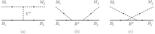
Figure 1: Leading order tree-level diagrams contributing to the meson-baryon interaction. Baryons and mesons are depicted by solid and dashed lines, respectively.

To describe the interaction we employ effective Lagrangians that describe the couplings of the vector meson to pseudoscalar mesons $(VPP)$ and baryons $(VBB)$, which are obtained using the hidden gauge formalism and assuming $SU(4)$ symmetry Hofmann:2005sw :

$$\mathcal{L}_{VPP}=ig\langle\left[\partial_{\mu}\phi,\phi\right]V^{\mu}\rangle,$$ (1)

$$\mathcal{L}_{VBB}=\frac{g}{2}\sum_{i,j,k,l=1}^{4}\bar{B}_{ijk}\gamma^{\mu}\left(V_{\mu,l}^{k}B^{ijl}+2V_{\mu,l}^{j}B^{ilk}\right),$$ (2)

where $\phi$ and $V_{\mu}$ represent the 16-plet pseudo-scalar field and the 16-plet vector field, respectively, and $\langle~{}\rangle$ denotes the $SU(4)$ trace in flavour space. The $g$ factor is a coupling constant which is related to the pion decay constant $(f=93~{}{\rm MeV})$ and a representative mass of a light vector meson from nonet $(m_{V})$ through the following relation,

$$g=\frac{m_{V}}{2f}.$$ (3)

Using the $VPP$ and $VBB$ vertices in the t-exchange diagram of Fig. 1 (a) one can obtain the s-wave interaction kernel $V_{ij}$ Hofmann:2005sw for the pseudoscalar meson baryon $(PB)$ interaction:

$$V_{ij}=g^{2}\sum_{v}C^{v}_{ij}\bar{u}(p_{j})\gamma^{\mu}u(p_{i})\frac{1}{t-m_{v}^{2}}\times$$

$$\Bigg{[}(k_{i}+k_{j})_{\mu}-\frac{k_{i}^{2}-k_{j}^{2}}{m_{v}}(k_{i}+k_{j})_{\mu}\Bigg{]},$$ (4)

where $p_{i/j}$ and $k_{i/j}$ denote the four-momentum of the baryons and mesons, respectively, and $i$, $j$ are the incoming and outgoing meson-baryon channels. The mass of the vector meson interchanged is $m_{v}$, and we approximate it as $m_{v}=m_{V}$, being equal for all of the vector mesons without charm quark and/or antiquark. For the charmed mesons we add a factor $\kappa_{c}=(m_{V}/m_{V}^{c})^{2}=1/4$ for $D^{*}$, $D_{s}^{*}$ mesons and $\kappa_{cc}=1/9$ for the $J/\psi$ in order to take account of their higher mass. This simplifies Eq. (II.1) into

$$V_{ij}=-C_{ij}\frac{1}{4f^{2}}\bar{u}(p_{j})\gamma^{\mu}u(p_{i})(k_{i}+k_{j})_{\mu},$$ (5)

where we have taken the limit $t\ll m_{V}$, which reduces the t-channel diagram to a contact term, and we have included the $\kappa_{c}$ and $\kappa_{cc}$ factors in the $C_{ij}$ matrix of coefficients, which will be provided later. This expression can be further simplified using the Dirac algebra up to $\mathcal{O}(p^{2}/M^{2})$, what leads to:

$$V_{ij}(\sqrt{s})=-C_{ij}\frac{1}{4f^{2}}\left(2\sqrt{s}-M_{i}-M_{j}\right)N_{i}N_{j},$$ (6)

where $M_{i}$, $M_{j}$ are the masses of the baryons in the channels $i$ and $j$, $N_{i}$ and $N_{j}$ are the normalization factors $N_{i}=\sqrt{(E_{i}+M_{i})/2M_{i}}$ and $E_{i}$, $E_{j}$ are the energies of the corresponding baryons. We note that although $SU(4)$ symmetry has been employed to obtain the $C_{ij}$ coefficients, our interaction potential is not $SU(4)$ symmetric, since we use the physical masses of mesons and baryons.

The interaction of vector mesons with baryons is built in a similar way and involves a three-vector $VVV$ vertex obtained from

$$\mathcal{L}_{VVV}=ig\langle[V^{\mu},\partial_{\nu}V_{\mu}]V^{\nu}\rangle.$$ (7)

One can see that in this case we can arrive to a similar expression as Eq. (6), but multiplied by the product of the polarization vectors, $\vec{\epsilon}_{i}\cdot\vec{\epsilon}_{j}$:

$$V_{ij}(\sqrt{s})=-C_{ij}\vec{\epsilon}_{i}\cdot\vec{\epsilon}_{j}\frac{1}{4f^{2}}\left(2\sqrt{s}-M_{i}-M_{j}\right)N_{i}N_{j}.$$ (8)

II.2 The $I=1/2~{}S=-2$ sector

In the $I=1/2~{}S=-2$ sector we have $9$ possible pseudoscalar-meson baryon (PB) channels, namely $\pi\Xi(1456)$, $\bar{K}\Lambda(1611)$, $\bar{K}\Sigma(1689)$, $\eta\Xi(1866)$, $\eta^{\prime}\Xi(2276)$, $\eta_{c}\Xi(4302)$, $\bar{D}_{s}\Xi_{c}(4437)$, $\bar{D}_{s}\Xi_{c}^{\prime}(4545)$, $\bar{D}\Omega(4565)$, where the values in parenthesis denote their thresholds. As can be seen, the channels with hidden charm are about $2~{}{\rm GeV}$ more massive compared with the lighter channels. Therefore we can expect these two regions to be essentially independent, making only a rather small effect on each other. The values of the $C_{ij}$ coefficients for the 9-channels are displayed in Table 1.

	$\pi\Xi$	$\bar{K}\Lambda$	$\bar{K}\Sigma$	$\eta\Xi$	$\eta^{\prime}\Xi$	$\eta_{c}\Xi$	$\bar{D}_{s}\Xi_{c}$	$\bar{D}_{s}\Xi_{c}^{\prime}$	$\bar{D}\Omega_{c}$
$\pi\Xi$	$2$	$\frac{3}{2}$	$\frac{1}{2}$	$0$	$0$	$0$	$0$	$0$	$\sqrt{\frac{3}{2}}\kappa_{c}$
$\bar{K}\Lambda$		$0$	$0$	$-\frac{3}{2}$	$0$	$0$	$-\frac{1}{2}\kappa_{c}$	$-\frac{\sqrt{3}}{2}\kappa_{c}$	$0$
$\bar{K}\Sigma$			$2$	$\frac{3}{2}$	$0$	$0$	$\frac{3}{2}\kappa_{c}$	$-\frac{\sqrt{3}}{2}\kappa_{c}$	$0$
$\eta\Xi$				$0$	$0$	$0$	$\kappa_{c}$	$\frac{1}{\sqrt{3}}\kappa_{c}$	$\frac{1}{\sqrt{6}}\kappa_{c}$
$\eta^{\prime}\Xi$					$0$	$0$	$\frac{1}{\sqrt{8}}\kappa_{c}$	$-\frac{1}{\sqrt{6}}\kappa_{c}$	$\frac{1}{\sqrt{3}}\kappa_{c}$
$\eta_{c}\Xi$						$0$	$\sqrt{\frac{3}{2}}\kappa_{c}$	$\frac{1}{\sqrt{2}}\kappa_{c}$	$-\kappa_{c}$
$\bar{D}_{s}\Xi_{c}$							$\kappa_{cc}-1$	$0$	$0$
$\bar{D}_{s}\Xi_{c}^{\prime}$								$\kappa_{cc}-1$	$-\sqrt{2}$
$\bar{D}\Omega_{c}$									$\kappa_{cc}$

Table 1: Coefficients $C_{ij}$ of the $PB$ interaction in the $I=1/2$, $S=-2$ sector

In the vector meson baryon (VB) sector, the allowed channels are $\rho\Xi(2089)$, $\bar{K}^{*}\Lambda(2010)$, $\bar{K}^{*}\Sigma(2087)$, $\omega\Xi(2101)$, $\phi\Xi(2338)$, $J/\psi\Xi(4415)$, $\bar{D}^{*}_{s}\Xi_{c}(4581)$, $\bar{D}^{*}_{s}\Xi_{c}^{\prime}(4689)$, $\bar{D}^{*}\Omega(4706)$, where we can again separate them in to groups, one with the light channels and the other with the heavy ones. In this case we can obtain the $C_{ij}$ coefficients directly from those in Table 1 using the following correspondences,

$$\begin{matrix}\pi\rightarrow\rho,&K\rightarrow K^{\ast},&\bar{K}\rightarrow\bar{K}^{\ast},&D\rightarrow D^{\ast},&\bar{D}\rightarrow\bar{D}^{\ast}\end{matrix}$$

$$\begin{matrix}\eta_{c}\rightarrow J/\psi,&\frac{1}{\sqrt{3}}\eta+\sqrt{\frac{2}{3}}\eta^{\prime}\rightarrow\omega,&-\sqrt{\frac{2}{3}}\eta+\frac{1}{\sqrt{3}}\eta^{\prime}\rightarrow\phi\ ,\end{matrix}$$ (9)

and these new coefficients are listed in Table 2.

	$\rho\Xi$	$\bar{K}^{*}\Lambda$	$\bar{K}^{*}\Sigma$	$\omega\Xi$	$\phi\Xi$	$J/\psi\Xi$	$\bar{D}^{*}_{s}\Xi_{c}$	$\bar{D}^{*}_{s}\Xi_{c}^{\prime}$	$\bar{D}^{*}\Omega_{c}$
$\rho\Xi$	$2$	$\frac{3}{2}$	$\frac{1}{2}$	$0$	$0$	$0$	$0$	$0$	$\sqrt{\frac{3}{2}}\kappa_{c}$
$\bar{K}^{*}\Lambda$		$0$	$0$	$-\frac{\sqrt{3}}{2}$	$\sqrt{\frac{3}{2}}$	$0$	$-\frac{1}{2}\kappa_{c}$	$-\frac{\sqrt{3}}{2}\kappa_{c}$	$0$
$\bar{K}^{*}\Sigma$			$2$	$\frac{\sqrt{3}}{2}$	$-\sqrt{\frac{3}{2}}$	$0$	$\frac{3}{2}\kappa_{c}$	$-\frac{\sqrt{3}}{2}\kappa_{c}$	$0$
$\omega\Xi$				$0$	$0$	$0$	$\kappa_{c}$	$\frac{1}{\sqrt{3}}\kappa_{c}$	$\frac{1}{\sqrt{6}}\kappa_{c}$
$\phi\Xi$					$0$	$0$	$\frac{1}{\sqrt{8}}\kappa_{c}$	$-\frac{1}{\sqrt{6}}\kappa_{c}$	$\frac{1}{\sqrt{3}}\kappa_{c}$
$J/\psi\Xi$						$0$	$\sqrt{\frac{3}{2}}\kappa_{c}$	$\frac{1}{\sqrt{2}}\kappa_{c}$	$-\kappa_{c}$
$\bar{D}_{s}\Xi_{c}$							$\kappa_{cc}-1$	$0$	$0$
$\bar{D}_{s}\Xi_{c}^{\prime}$								$\kappa_{cc}-1$	$-\sqrt{2}$
$\bar{D}\Omega_{c}$									$\kappa_{cc}$

Table 2: Coefficients $C_{ij}$ of the $VB$ interaction in the $I=1/2$, $S=-2$ sector

Note that for the light $PB$ sector, due to the fact that all $C_{5j}$ coefficients with $j\leq 5$ are zero, we formally have only $4$ coupled channels, while this is not the case for the light $VB$ sector which remains with $5$ coupled channels in this case.

II.3 Dynamically generated resonances

The sought resonances are dynamically generated as poles of the scattering amplitude $T_{ij}$, which is unitarized via the on-shell Bethe-Salpeter equation in coupled channels. This corresponds to performing the resumation of loop diagrams to an infinite order (see Fig. 2),

$$T_{ij}=V_{ij}+V_{il}G_{l}V_{lj}+V_{il}G_{l}V_{lk}G_{k}V_{kj}+...=V_{ij}+V_{il}G_{l}T_{lj}$$ (10)

where $G_{l}$ is the loop function, which is given by

$$G_{l}=i\int\frac{d^{4}q}{(2\pi)^{4}}\frac{2M_{l}}{(P-q)^{2}-M_{l}^{2}+i\epsilon}\frac{1}{q^{2}-m_{l}^{2}+i\epsilon}.$$ (11)

The masses $M_{l}$ and $m_{l}$ correspond to those of the baryon and meson of the $l$ channel, respectively, $P=p+k=(\sqrt{s},0)$ is the total four momenta in the c.m. frame, and $q$ denotes the four momentum in the intermediate loop. We factorize the $V$ and $T$ matrices on-shell out of the integrals in Eq. (10) Montana:2017kjw , hence obtaining the following algebraic matrix expression for the scattering amplitude,

$$T=(1-VG)^{-1}V.$$ (12)

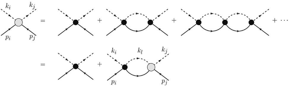
Figure 2: Diagrams that represent the Bethe-Salpeter equation. The empty circle corresponds to the $T_{ij}$ matrix elements, the black ones represent the $V_{ij}$ potential and the loops are the $G_{l}$ propagator functions.

Note that the sum over the polarization vector in the case of the vector meson baryon interaction, eq. (8), gives Montana:2017kjw

$$\sum_{pol}\epsilon_{i}\epsilon_{j}=\delta_{ij}+\frac{q_{i}q_{j}}{M_{V}^{2}},$$ (13)

where, consistently with our model, we neglect the $q^{2}/M_{V}^{2}$ term, thus all $\vec{\epsilon}_{i}\vec{\epsilon}_{j}$ factorize out from all terms in the Bethe-Salpeter equation.

II.4 Loop function

It is important to know that the loop function in Eq. (11) diverges logarithmically, so we must renormalize it. We can employ the cut-off method, which consists in changing the infinity at the upper $q$ limit to one large enough cut-off momentum $\Lambda$

$$G_{l}^{cut}=\int_{0}^{\Lambda}\frac{q^{2}dq}{4\pi^{2}}\frac{2M_{l}(E_{l}+\omega_{l})}{E_{l}\omega_{l}[(P^{0})^{2}-(E_{l}+\omega_{l})^{2}+i\epsilon]},$$ (14)

where $E_{l}=\sqrt{\vec{q}^{\,2}+M_{l}^{2}}$ and $\omega_{l}=\sqrt{\vec{q}^{\,2}+m_{l}^{2}}$.

A different option is using the dimensional regularisation scheme, which gives rise to the following analytic expression

$$G_{l}= \frac{2M_{l}}{16\pi^{2}}\Big{\{}a_{l}(\mu)+\ln\frac{M_{l}^{2}}{\mu^{2}}+\frac{m_{l}^{2}-M_{l}^{2}+s}{2s}\ln\frac{m_{l}^{2}}{M_{l}^{2}}+$$ (15)

$$+\frac{q_{l}}{\sqrt{s}}\left[\ln\left(s-(M_{l}^{2}-m_{l}^{2}\right)+2q_{l}\sqrt{s})\right.$$

$$\phantom{\frac{q_{l}}{\sqrt{s}}~{}~{}}+\ln\left(s+(M_{l}^{2}-m_{l}^{2}\right)+2q_{l}\sqrt{s})$$

$$\phantom{\frac{q_{l}}{\sqrt{s}}~{}~{}}-\ln\left(-s+(M_{l}^{2}-m_{l}^{2}\right)+2q_{l}\sqrt{s})$$

$$\phantom{\frac{q_{l}}{\sqrt{s}}~{}~{}}\left.-\ln\left(-s-(M_{l}^{2}-m_{l}^{2}\right)+2q_{l}\sqrt{s})\right]\Big{\}},$$

were $q_{l}$ is the on-shell three-momentum of the meson in the loop, and we have introduced a subtraction constant, $a(\mu)$, at the regularisation scale $\mu$. In this work we will take $\mu=1000~{}{\rm MeV}$ consistently with previous approaches Montana:2017kjw . Although these two expression for the loop function, (14) and (15), give a rather different result at low (sub-threshold) and high energies, they can be rather similar in the threshold region of the corresponding channels. The value of the subtraction constant that produces the same loop function at threshold as that obtained with a cut-off $\Lambda$ is determined by

$$a_{l}({\mu})=\frac{16\pi^{2}}{2M_{l}}\left(G_{l}^{\text{cut}}(\Lambda)-G_{l}(\mu,a_{l}=0)\right).$$ (16)

Some mesons in the considered channels have a large width $(\Gamma_{\rho}=149.4~{}{\rm MeV}$ and $\Gamma_{K^{*}}=50.5~{}{\rm MeV}$), but $G_{l}$ in Eq. (15) does not take into account this fact. Therefore, in order to implement the meson width we convolute this function with the mass distribution of the particle. This method has been used in Montana:2017kjw ; Oset:2010tof and the resulting loop function for these channels becomes:

$$\tilde{G}_{l}(s)=-\frac{1}{N}\int_{(m_{l}-2\Gamma_{l})^{2}}^{(m_{l}+2\Gamma_{l})^{2}} \frac{d\tilde{m}_{l}^{2}}{\pi}{\rm\,Im\,}\frac{1}{\tilde{m}_{l}^{2}-m_{l}^{2}+i\,m_{l}\Gamma(\tilde{m}_{l})}$$

$$\times G_{l}\left(s,\tilde{m}_{l}^{2},M_{l}^{2}\right),$$ (17)

where we extend the integration limits up to twice the meson width on either side of the mass, and the normalisation factor $N$ is

$$N=\int_{(m_{l}-2\Gamma_{l})^{2}}^{(m_{l}+2\Gamma_{l})^{2}}d\tilde{m}_{l}^{2}\left(-\frac{1}{\pi}\right){\rm\,Im\,}\frac{1}{\tilde{m}_{l}^{2}-m_{l}^{2}+i\,m_{l}\Gamma(\tilde{m}_{l})}\ .$$ (18)

The energy-dependent width is given by

$$\Gamma(\tilde{m}_{l})=\Gamma_{l}\frac{m_{l}^{5}}{\tilde{m}_{l}^{5}}\frac{\lambda^{3/2}(\tilde{m}_{l}^{2},m_{1}^{2},m_{2}^{2})}{\lambda^{3/2}(m_{l}^{2},m_{1}^{2},m_{2}^{2})}\,\theta(\tilde{m}_{l}-m_{1}-m_{2}),$$ (19)

where $m_{1}$ and $m_{2}$ are the masses of the lighter mesons into which the vector meson decays and $\lambda$ is the Källén function $\lambda(x,y,z)=(x-(\sqrt{y}+\sqrt{z})^{2})(x-(\sqrt{y}-\sqrt{z})^{2})$.

Then, the obtained scattering amplitude ($T$) can be analytically continued to the complex plane of $s$. The dynamically generated resonances appear as poles of the amplitude $T_{ij}$ in the so-called second Riemann sheet, obtained by using the following rotation of the loop function Montana:2017kjw :

$$G_{l}^{\text{II}}(\sqrt{s}+i\epsilon)=G_{l}(\sqrt{s}+i\epsilon)+i\frac{q_{l}}{4\pi\sqrt{2}}.$$ (20)

Around the pole position $\sqrt{s_{p}}=M_{p}+i\Gamma_{p}/2$ the scattering amplitude can be approximated as

$$T_{ij}(\sqrt{s})\simeq\frac{g_{i}g_{j}}{\sqrt{s}-\sqrt{s_{p}}},$$ (21)

from which we can obtain the coupling constants, $g_{i}$, of the pole/resonance for all channels. In addition, we calculate the compositeness defined as:

$$\chi_{i}=\Bigl{\lvert}g_{i}^{2}\frac{\partial G_{i}(\sqrt{s})}{\partial\sqrt{s}}\Bigr{\rvert}_{\sqrt{s}=\sqrt{s_{p}}},$$ (22)

which approximately gives the contribution of the $i$-th channel meson-baryon component in a given resonance.

III Molecular resonances in S=-2 sector

III.1 Light sector

We first discuss the results of the light channels of the pseudoscalar meson baryon interaction, where we employ the dimensional regularisation scheme to compute the loop function. The values of the unknown subtraction constants are determined by imposing the loop function to coincide, for a regularisation scale of $\mu=1000~{}{\rm MeV}$, with the loop cut-off function with $\Lambda=800~{}{\rm MeV}$ at the corresponding threshold (Eq. (16)). We chose this value as it corresponds to the mass of the interchanged vector meson on the t-channel diagram which is integrated out when we take the $t\to 0$ limit. We will refer to this procedure as Model PB 1.

Of course, first of all we have checked that our idea of separation between light and heavy channels works. As a typical example of the obtained effect, in Fig. 3 we show the sum over all $j$ channels of the modulus of the PB scattering amplitude from the given channel $j$ into $\bar{K}\Sigma$, i.e. $\sum_{j}\,|T_{3j}|$. As expected, the effect of heavy channels is negligible.

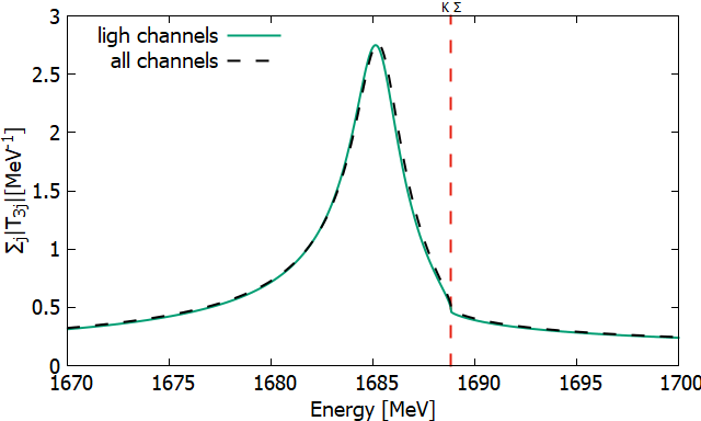
Figure 3: The curves represent the sum over all $j$ channels of the modulus of the PB scattering amplitude, $|T_{3j}|$, obtained in Model PB1. The vertical coloured dashed lines represent the location of the thresholds of the different channels. The solid line shows the results when the heavy channels are neglected and the dashed one presents the results using all 9 the channels.

The results of our calculations within Model PB1 are shown in Fig. 4, where we represent $\sum_{j}|T_{ij}|$ as a function of the c.m. energy for all different $i$ channels in different colours. These amplitudes show a broad peak (barely visible) at low energies and a narrower one right below the $\bar{K}\Sigma$ threshold. This behaviour is the reflection of two poles, the properties of which are shown in Table 3. Note that these states have a well defined spin-parity of $J^{\pi}=\frac{1}{2}^{-}$, since they are formed with a scalar meson $(J^{\pi}=0^{-})$ and a baryon $(J^{\pi}=\frac{1}{2}^{+})$ interacting in s-wave.

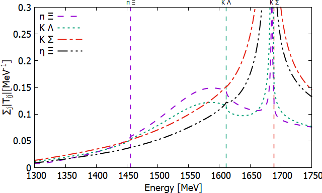
(a)

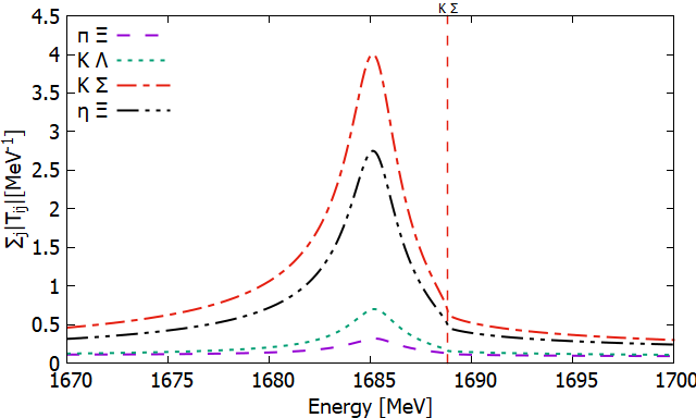
(b)

Figure 4: Solid lines represent the sum over all $j$ channels of the modulus of the PB scattering amplitude, $|T_{ij}|$, for a fixed channel $i$, obtained in Model PB 1. Subfigure (b) shows the region of the second pole with more details at higher scale. The vertical dashed lines represent the location of the thresholds of the different channels.

$0^{-}\oplus\frac{1}{2}^{+}$ interaction in the $(I,S)=(\frac{1}{2},-2)$ sector
Model PB 1
$M(\rm MeV)$			$1570.53$		$1685.18$
$\Gamma({\rm MeV})$			$174.04$		$2.28$
	$a_{i}$	$\Lambda$	$|g_{i}|$	$\chi_{i}$	$|g_{i}|$	$\chi_{i}$
$\pi\Xi(1456)$	-1.51	800	2.44	0.428	0.12	0.001
$\bar{K}\Lambda(1611)$	-1.32	800	1.91	0.169	0.27	0.006
$\bar{K}\Sigma(1689)$	-1.27	800	0.71	0.016	1.54	0.815
$\eta\Xi(1866)$	-1.47	800	0.49	0.004	1.06	0.029
Model PB 2
$M(\rm MeV)$			$1600.55$		$1685.40$
$\Gamma({\rm MeV})$			$228.64$		$2.60$
	$a_{i}$	$\Lambda$	$|g_{i}|$	$\chi_{i}$	$|g_{i}|$	$\chi_{i}$
$\pi\Xi(1456)$	-1.30	630	2.70	0.501	0.15	0.001
$\bar{K}\Lambda(1611)$	-1.00	740	2.21	0.214	0.27	0.006
$\bar{K}\Sigma(1689)$	-1.27	800	0.86	0.025	1.53	0.822
$\eta\Xi(1866)$	-1.47	800	0.42	0.003	1.02	0.027

Table 3: Position, subtraction constants, cut off, couplings and compositeness of the $\Xi$ states generated with the light channels of the PB interaction.

We can observe that the lowest generated resonance couples strongly to the $\pi\Xi$ and $\bar{K}\Lambda$ channels, which are open for decay, what actually explains its rather large width. In the PDG PDG one can find a state with similar mass, $\Xi(1620)$, which was seen decaying into the $\pi\Xi$ channel (Tab. 4). Even if our state is $50~{}{\rm MeV}$ lighter and its width is larger, we can see the potential of our model to generate a state in this region.

As it can also be seen in Table 3 our heavier state mostly couples to the $\bar{K}\Sigma$ and $\eta\Xi$ channels and it has a mass of $1685~{}{\rm MeV}$. According to PDG data there exists a $\Xi(1690)$ state at $1690\pm 10~{}{\rm MeV}$ with a width of $20\pm 15~{}{\rm MeV}$ (Tab. 4), which is compatible with our result.

PDG data					Model PB 1		Model PB 2
State	Evidence	$J^{\pi}$	$M({\rm MeV})$	$\Gamma({\rm MeV})$	$M({\rm MeV})$	$\Gamma({\rm MeV})$	$M({\rm MeV})$	$\Gamma({\rm MeV})$
$\Xi(1620)$	**	-	$\sim 1620$	$32^{+8}_{-9}$	$1570.53$	$174.53$	$1600.55$	$228.65$
$\Xi(1690)$	***	-	$1690\pm 10$	$20\pm 15$	$1685.18$	$2.28$	$1685.40$	$2.60$
PDG					Model VB 2		Model VB 3
$\Xi(1820)$	***	$\frac{3}{2}^{-}$	$1823\pm 5$	$24^{+15}_{-10}$	$1823.12$	$0.66$	$-$	$-$
$\Xi(1950)$	***	-	$1950\pm 15$	$60\pm 20$	$1949.23$	$0.232$	$1935.99$	$8.29$
							$1964.09$	$4.92$

Table 4: Experimental information for the $\Xi(1620)$, $\Xi(1690)$, $\Xi(1820)$, $\Xi(1950)$ resonances and the mass and width for the states generated with four different models.

Looking at the results, it is natural to think that we can modify the values of the subtraction constants within a reasonable range in order to accommodate the generated states to the experimental data. Therefore, we relax the condition for our loop function has to be equal to the cut-off loop function with $\Lambda=800~{}{\rm MeV}$ at the corresponding threshold Montana:2017kjw . By doing that we define a new model, called PB 2. The results of new calculations within Model PB2 are shown in Fig. 5 and in Table 3. We can see that our lighter resonance now appears at higher mass and it is much wider, while the heavier resonance is generated with a similar mass and with a slightly larger width. Looking at Table 4 we can see that now the mass of the light state is closer to the experimental energy of the $\Xi(1620)$. In this model, none of the equivalent cut-off values for the subtractions constants employed are smaller than $\Lambda=630~{}{\rm MeV}$, which is a reasonable lower limit value.

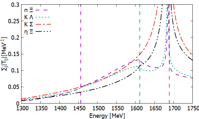
(a)

Figure 5: Solid lines represent the sum over all $j$ channels of the modulus of the PB scattering amplitude, $|T_{ij}|$, for a fixed channel $i$, obtained in Model PB 2. The vertical dashed lines represent the location of the thresholds of the different channels.

Reviewing the literature Sekihara:2015qqa ; Kaiser:1995eg ; Oset:1997it ; Ramos:2002xh ; Garcia-Recio:2003ejq ; Gamermann:2011mq ; Nishibuchi:2023acl ; Nishibuchi:2022zfo ; Nishibuchi:2023nvi one can note that all the models based only on a leading interaction term in the potential, the so called Weinberg-Tomozawa term, see eq. (6), although can dynamically generate two poles, but the features of those could not reproduce the experimental masses and widths of $\Xi(1620)$ and $\Xi(1690)$ at the same time. Furthermore, the width of the $\Xi(1690)$ remains always rather small, around a few MeV. And our calculations do also show all these features.

In principle, the $\Xi(1620)$ resonance can be reproduced very well Nishibuchi:2023acl ; Nishibuchi:2022zfo ; Nishibuchi:2023nvi , but only allowing some of the subtracting constants to take unnatural-size values.

This limitations can be overcame, if one takes into consideration also the s- and u-channel Born diagrams and the NLO contribution, as it was done in Feijoo:2023wua ; Magas:2024mba ; Sarti:2023wlg , where both $\Xi(1620)$ and $\Xi(1690)$ are well reproduced by the model.

We proceed now to discuss the results for the vector meson baryon interaction, where we construct the model VB 1 in a similar way as to the model PB 1, i. e. using a regularisation scale of $\mu=1000~{}{\rm MeV}$ and requesting that our loop function, regularized via dimensional regularization, for each channel should have the same value at the threshold as that computed with cut-off $\Lambda=800~{}{\rm MeV}$. Using this model we produce the amplitude displayed in Fig. 6, which has two poles with properties listed in Table 5. Note that each of these states forms a degenerate spin-parity doublet with $J^{\pi}=\frac{1}{2}^{-}$, $J^{\pi}=\frac{3}{2}^{-}$, since they are produced from the interaction of a vector meson $(J^{\pi}=1^{-})$ an a baryon $(J^{\pi}=\frac{1}{2}^{+})$ in s-wave.

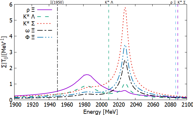
Figure 6: Solid lines represent the sum over all $j$ channels of the modulus of the VB scattering amplitude, $|T_{ij}|$ for a fixed channel $i$, obtained in Model VB 1. The vertical coloured dashed lines represent the location of the thresholds of the different channels and the black one represents the mass position of the $\Xi(1950)$.

$1^{-}\oplus\frac{1}{2}^{+}$ interaction in the $(I,S)=(\frac{1}{2},-2)$ sector
Model VB 1
M(Mev)			1985.95		2028.40
$\Gamma({\rm MeV})$			29.23		6.86
	$a_{i}$	$\Lambda$	$|g_{i}|$	$\chi_{i}$	$|g_{i}|$	$\chi_{i}$
$\rho\Xi(2089)$	-1.50	800	3.39	0.610	0.24	0.004
$\bar{K}^{*}\Lambda(2010)$	-1.42	800	1.82	0.358	0.52	0.0490
$\bar{K}^{*}\Sigma(2087)$	-1.46	800	0.98	0.047	2.97	0.629
$\omega\Xi(2101)$	-1.50	800	0.54	0.014	1.30	0.114
$\phi\Xi(2338)$	-1.57	800	0.75	0.012	1.80	0.077
Model VB 2
M(Mev)			1823.12		1949.23
$\Gamma({\rm MeV})$			0.66		0.232
	$a_{i}$	$\Lambda$	$|g_{i}|$	$\chi_{i}$	$|g_{i}|$	$\chi_{i}$
$\rho\Xi(2089)$	-2.19	1440	3.48	0.323	0.16	0.001
$\bar{K}^{*}\Lambda(2010)$	-2.00	1300	2.07	0.131	0.66	0.035
$\bar{K}^{*}\Sigma(2087)$	-1.87	1140	1.16	0.033	3.15	0.509
$\omega\Xi(2101)$	-1.50	800	0.41	0.004	1.43	0.100
$\phi\Xi(2338)$	-1.80	990	0.56	0.005	1.98	0.100
Model VB 3
M(Mev)			1935.99		1964.09
$\Gamma({\rm MeV})$			8.29		4.92
	$a_{i}$	$\Lambda$	$|g_{i}|$	$\chi_{i}$	$|g_{i}|$	$\chi_{i}$
$\rho\Xi(2089)$	-1.74	990	2.88	0.335	1.43	0.096
$\bar{K}^{*}\Lambda(2010)$	-1.42	800	1.41	0.116	1.53	0.186
$\bar{K}^{*}\Sigma(2087)$	-1.82	1090	2.58	0.250	2.66	0.309
$\omega\Xi(2101)$	-1.50	800	0.41	0.006	1.45	0.092
$\phi\Xi(2338)$	-1.85	1040	0.56	0.006	2.00	0.081

Table 5: Position, subtraction constants, cut off, couplings and compositeness of the $\Xi$ states generated with the light channels of the VB interaction.

As it can be seen in Table 5, our lighter state couples strongly to the $\rho\Xi$ channel. Note that this state, although its mass is lower than all the thresholds, has a non-zero width. This is because we take into account the width of the $\rho$ and the $\bar{K}^{*}$ in the loop function. For the higher energy peak we can see that it strongly couples to the $\bar{K}^{*}\Sigma$ channel. In the PDG data one can find two states in this region, the $\Xi(1820)$ and the $\Xi(1950)$ (Tab. 4). The first state has a known spin-parity $J^{\pi}=\frac{3}{2}^{-}$, which is compatible with our model.

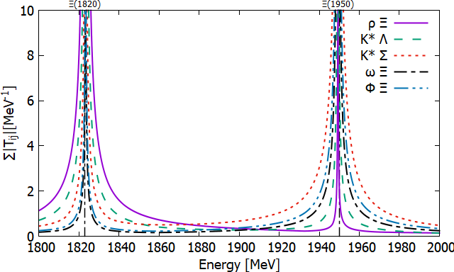
Figure 7: Solid lines represent the sum over all $j$ channels of the modulus of the VB scattering amplitude, $|T_{ij}|$ for a fixed channel $i$, obtained in Model VB 2. The vertical coloured dashed lines represent the location of the thresholds of the different channels and the black one represents the mass position of the $\Xi(1820)$ and the $\Xi(1950)$.

Similarly to what we did in PB case, we will modify our subtraction constants within a reasonable range trying to adjust our results to the experimental data. Modifying the values of the subtraction constants we build model VB 2, which produces two resonances at energies compatible with the experimental masses of $\Xi(1829)$ and $\Xi(1950)$ (see Fig. 7 and Table 5). We note that the values of the equivalent cut-offs for the subtractions constants employed are not larger than $\Lambda=1500~{}{\rm MeV}$, which is a reasonable upper limit value (Tab. 5). However, the widths of these obtained resonances are much smaller than experimental ones. Potentially this problem might be solved if we developed a model which would couple the VB channels with the PB ones, since this would open more light channels in which these resonances could decay, increasing their width. Such a coupling was studied in Garzon:2012np , and indeed it generated some increase of the width for the lower lying resonance.

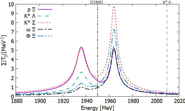
Figure 8: Solid lines represent the sum over all $j$ channels of the modulus of the VB scattering amplitude, $|T_{ij}|$ for a fixed channel $i$, obtained in Model VB 3. The vertical coloured dashed lines represent the location of the thresholds of the different channels and the black one represents the mass position of the $\Xi(1950)$.

Another possibility to adjust our model to the experimental data is to generate both resonances in the energy region where the $\Xi(1950)$ appears. As described in the PDG PDG this state could be representing more than one $\Xi$ resonance, eventually merging into an apparent wide peak. With such a motivation we generated model VB 3, which, as can be seen in Fig. 8 and Table 5, produces two states close to the experimental position of the $\Xi(1950)$. Note that for this model we only need to modify three subtraction constants and the equivalent cut-off values are not larger than $1100~{}{\rm MeV}$ for all the channels. If our resonances were a bit wider, what can be achieved, for example, by coupling our VB channels with the PB ones, as discussed above, they would produce just one, but rather wide, peak in the experimental data, as it happens for $\Lambda(1405)$.

III.2 Heavy sector

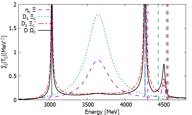
Figure 9: Solid lines represent the sum over all $j$ channels of the modulus of the PB scattering amplitude, $|T_{ij}|$ for a fixed channel $i$, obtained applying the dimensional regularisation scheme for the loop function. The vertical dashed lines represent the location of the thresholds of the different channels.

Let us now discuss the results in the heavy sector, where there are only four channels. In a rather brief form these results have already been published in ref Marse-Valera:2022khy , while in this section we will show more results and more details of the calculations.

We will start in a similar way as we did in the previous section. First of all, we set the regularisation scale to $\mu=1000~{}{\rm MeV}$ and the subtraction constants are evaluated for all the channels mapping the loop function to the value obtained for a cut-off of $\Lambda=800~{}{\rm MeV}$ at the threshold of each channel. In such a way four peaks are generated, as we can see in Fig. 9.

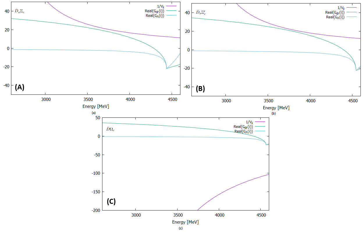
Figure 10: The purple line represents the inverse of the diagonal term of the potential, the green line shows the loop function of the same channel, computed using a dimensional regularisation scheme, and the blue line is similar to the green one, but computed using a cut-off scheme. In (a) we have the $\bar{D}_{s}\Xi_{c}$ channel, in (b) the $\bar{D}_{s}\Xi_{c}^{\prime}$ and in (c) the $\bar{D}\Omega_{c}$.

Analyzing these results wee observe that the first three peaks couple very strongly to $\bar{D}_{s}~{}\Xi^{\prime}_{c}$ and/or to $\bar{D}_{s}~{}\Xi_{c}$, what is very suspicious, since the diagonal elements of the potential for these channels are repulsive ($C_{ii}<0$, see Tab. 1). This might be an indication that these peaks/poles are fake; these might be mathematical artifacts of the dimensional regularization scheme, that have been already seen before. To illustrate the problem, we present in Figs. 10 the inverse of the diagonal potential and the real part of the loop function calculated both using the dimensional regularisation and the cut-off methods for three heaviest channels. Note that according to Eq. (12), a pole is generated when $VG\sim 1$. As we can see in Figs. 10 (a) and (b) the inverse of the potential and the real part of the dimensional regularized loop function almost intersect in a region where the potential is repulsive. Thus, these states, which mostly couple to $\bar{D}\Xi_{c}$ and $\bar{D}\Xi_{c}^{\prime}$, are only mathematical solutions of our equation, but do not represent any physical state. Fig. 10 also shows that to avoid such fake poles we should use the cut-off scheme to compute the loop functions.

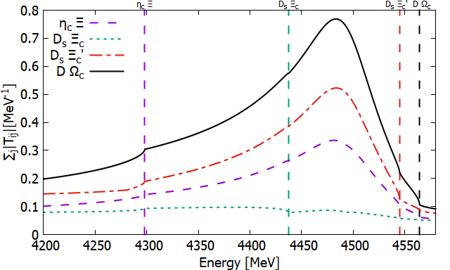
Figure 11: Solid lines represent the sum over all $j$ channels of the modulus of the PB scattering amplitude, $|T_{ij}|$, obtained using the cut-off model to compute the loop function. The vertical dashed lines represent the location of the thresholds of the different channels.

As can be seen in Fig. 11, using a cut-off model with $\Lambda=800~{}{\rm MeV}$, we make the fake poles disappear and, as expected, only the pole at higher energy remains. This one strongly couples to the $\bar{D}\Omega_{c}$ and $\bar{D}_{s}\Xi_{c}^{\prime}$ channels (see Table 6). This state, which would be a pentaquark with double strangeness ($P_{\Psi_{ss}}^{\Xi}$) has a well defined spin-parity $J^{\pi}=\frac{1}{2}^{-}$ as it is generated from the PB interaction in s-wave.

$0^{-}\oplus\frac{1}{2}^{+}$ interaction in the $(I,S)=(0,-2)$ sector
M(Mev)		4493.35
$\Gamma({\rm MeV})$		73.67
	$\Lambda$	$g$	$|g_{i}|$	$\chi_{i}$
$\eta_{c}\Xi(4302)$	800	$-1.60+0.34i$	1.63	0.220
$\bar{D}_{s}\Xi_{c}(4437)$	800	$-0.17+0.27i$	0.32	0.019
$\bar{D}_{s}\Xi_{c}^{\prime}(4545)$	800	$-2.41+0.58i$	2.48	0.398
$\bar{D}\Omega_{c}(4564)$	800	$3.59-0.77i$	3.67	0.711

Table 6: Position, cut off, couplings and compositeness of the $\Xi$ state generated with the heavy channels of the PB interaction.

It is very interesting to look for the origin of this resonance. Checking Table 1 we can see that there is only one attractive diagonal term, for $\bar{D}\Omega_{c}$ channel, and although it is positive (i.e. attractive in our parameterization) itis still rather small small $(C_{99}=1/9)$. Such an attraction is not sufficient to generate a resonance state (what was check performing uncoupled calculations). Thus, this resonance is generated in a rather unusual way, via the non-diagonal terms of the interaction. The $\bar{D}\Omega_{c}-\bar{D}_{s}\Xi_{c}^{\prime}$ interaction, $C_{98}=-\sqrt{2}$, is strong enough to produce a bound state via the coupled-channels. To check this point, we added a $\gamma$ factor, $C_{89}\to C_{89}^{\prime}=-\gamma\sqrt{2}$, which can be varied to see the effect of this off-diagonal term in details. In Fig. 12 we can clearly see the effect of this term - for smaller values of $C_{89}^{\prime}$ ($\gamma\sim 0.5$) the resonance state is not generated.

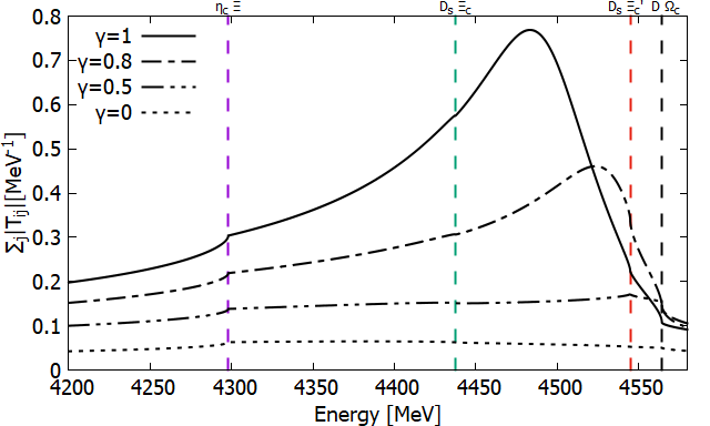
Figure 12: Solid lines represent the sum over all $j$ channels of the modulus of the PB scattering amplitude, $|T_{ij}|$, for $i=\bar{D}\Omega_{c}$ and for different $\gamma$’s ($C_{89}\to C_{89}^{\prime}=\gamma C_{89}$). Loop function is calculated with a cut-off scheme as in Fig. 11. The vertical dashed lines represent the location of the thresholds of the different channels.

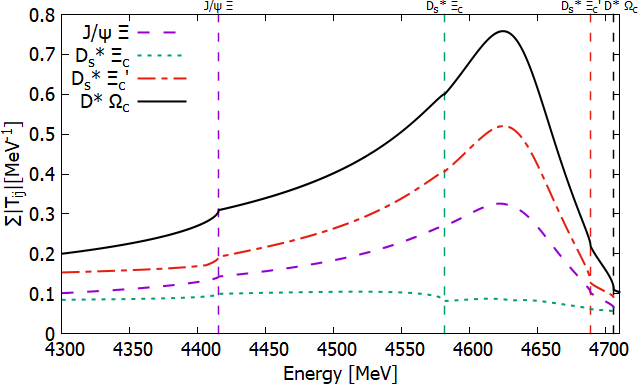
Figure 13: Solid lines represent the sum over all $j$ channels of the modulus of the VB scattering amplitude, $|T_{ij}|$ for a fixed channel $i$, obtained using the cut-off scheme to compute the loop function. The vertical dashed lines represent the location of the thresholds of the different channels.

We now present our results in the heavy VB sector. In the similar way as in the PB sector, the use of dimension regularization for the loop function leads to some fake nonphysical poles, which have been eliminated by the use of the cut-off method. Finally, only one resonance state remains, which couples strongly to $\bar{D}^{*}\Omega_{c}$ and $\bar{D}_{s}^{*}\Xi_{c}^{\prime}$, see Fig. 13 and Table 7. Similarly to the PB sector this state can be formed due to the large value of $C_{89}$, what is illustrates in Fig. 14. Note that this state is degenerate in spin-parity, can be either $J^{P}=\frac{1}{2}^{-}$ or $J^{P}=\frac{3}{2}^{-}$, since we have a vector-meson $(J^{P}=1^{-})$ interacting with a baryon $(J^{P}=\frac{1}{2}^{+})$ in s-wave.

$1^{-}\oplus\frac{1}{2}^{+}$ interaction in the $(I,S)=(0,-2)$ sector
M(Mev)		4633.38
$\Gamma({\rm MeV})$		79.58
	$\Lambda$	$g$	$|g_{i}|$	$\chi_{i}$
$J/\psi\Xi(4415)$	800	$-1.62+0.38i$	1.66	0.252
$\bar{D}_{s}^{*}\Xi_{c}(4581)$	800	$-0.143+0.32i$	0.34	0.022
$\bar{D}_{s}^{*}\Xi_{c}^{\prime}(4689)$	800	$-2.49+0.67i$	2.58	0.406
$\bar{D}^{*}\Omega_{c}(4706)$	800	$3.67+0.89i$	3.78	0.740

Table 7: Position, cut off, couplings and compositeness of the $\Xi$ states generated with the heavy channels of the VB interaction.

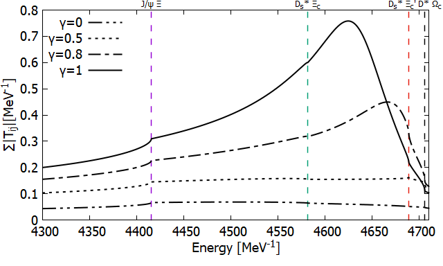
Figure 14: Solid lines represent the sum over all $j$ channels of the modulus of the VB scattering amplitude, $|T_{ij}|$, for $i=\bar{D}^{*}\Omega_{c}$ and for different $\gamma$’s ($C_{89}\to C_{89}^{\prime}=\gamma C_{89}$). Loop function is calculated with a cut-off scheme as in Fig. 13. The vertical dashed lines represent the location of the thresholds of the different channels.

We also have checked that the variations of cut off value, of $\kappa_{c}$ and $\kappa_{cc}$ parameters (related to explicit violation of SU(4) symmetry) lead to some variations of the resonance position and properties, but the appearance of a pole is a robust outcome in all calculations both for PB and VB cases Marse-Valera:2022khy .

Thus we have shown that in a simple model with realistic parameters we have been able to dynamically generate three pentaquarks with doubly strangeness and hidden charm. Shortly after our first results have been published Marse-Valera:2022khy , another study performed with a similar model appeared Roca:2024nsi , where similar pentaquarks have been generated in the same mass region, but with much smaller widths. The main reason for this differences, as it is explained by the authors of Roca:2024nsi , is the $-1/\sqrt{3}$ factor that appears in their $C{ij}$ constants for the $\eta_{c}\Xi$ and $J/\psi\Xi$ channels. We checked that by adopting our matrix to the values Roca:2024nsi , our model generates resonance practically at the same place, but with a smaller width of about $22~{}{\rm MeV}$. Our states are still generated at a bit higher energies, what makes it easier for them to decay into the $\eta_{c}\Xi$ or the $J/\psi\Xi$ channels increasing their width.

IV The $\Xi_{b}\to J/\Psi\phi\Xi$ decay: formalism

IV.1 Dalitz Plot

As it was mentioned earlier in Ref. Oset:2024fbk the authors suggest the $\Xi_{b}^{0}\to\eta\eta_{c}\Xi^{0}$ and $\Omega_{b}^{-}\to K^{-}\eta_{c}\Xi^{0}$ decays in order to observe the $P_{css}$ with $I(J^{P})=\frac{1}{2}(\frac{1}{2}^{-})$ generated via pseudoscalar-baryon interaction. In this study the authors used a model from ref. Roca:2024nsi , i.e. with narrow $P_{css}$ pentaquarks.

In this chapter we will study the $\Xi_{b}\to\Xi~{}J/\psi~{}\phi$ decay, as a possible reaction to look for a double strangeness pentaquark via vector-baryon channel. And first of all, we will look at Dalitz plots, i.e. at the two-body invariant mass distributions of the three possible pairs of particles $(J/\psi\phi,~{}J/\psi\Xi,~{}\phi\Xi)$, what will make clear that there exists a good possibility to detect exotic hadrons and not only pentaquarks $P_{css}$.

From the relativistic kinematics of a three body decay the Dalitz plot can be generated, which represents the available invariant mass for the different pairs of particles. So if we explore the Dalitz plots for the $\Xi_{b}\to\Xi~{}J/\psi~{}\phi$ reaction (Fig. 15) we can see whether the different exotic resonances lie inside the kinematically allowed region.

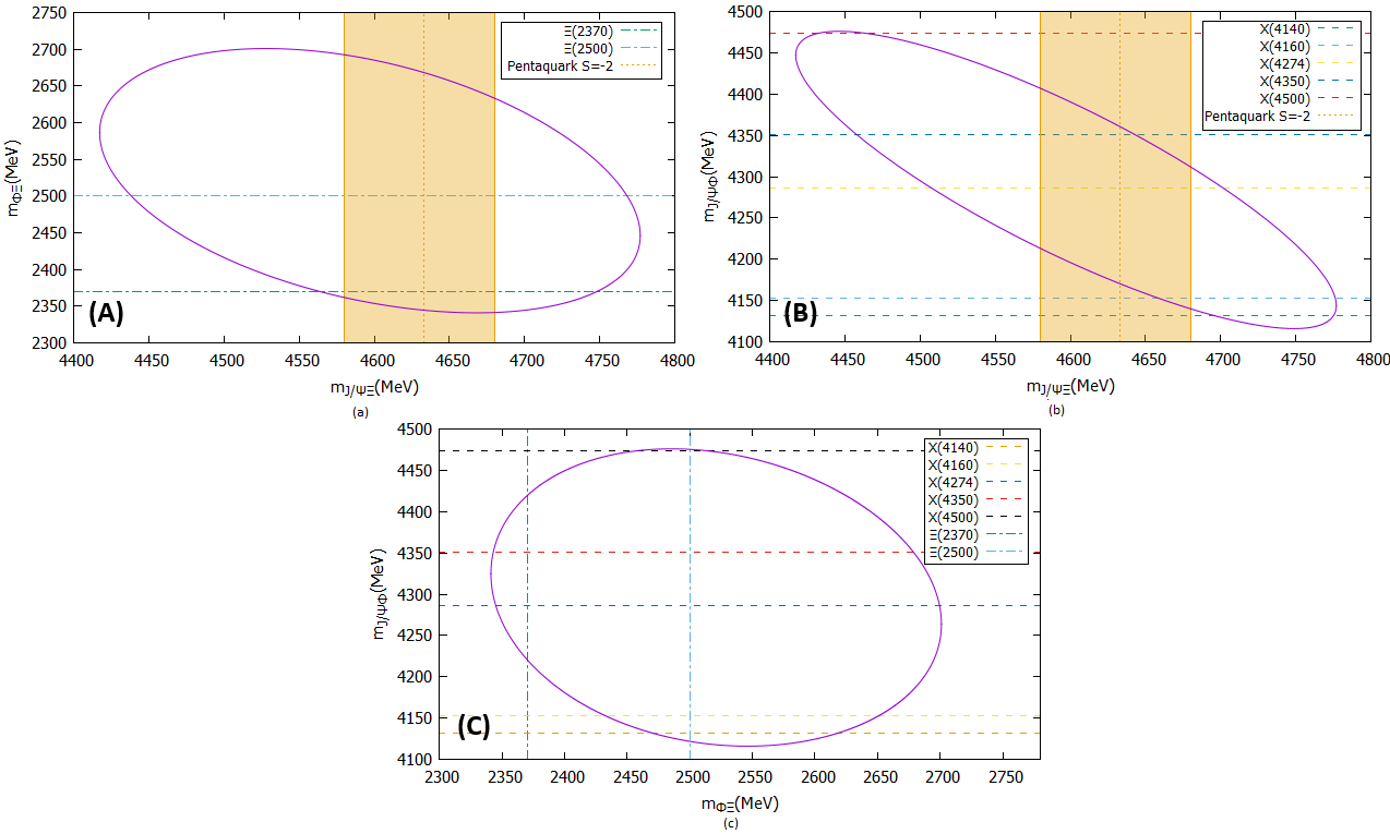
Figure 15: The solid lines represent the Dalitz plot for $M_{\phi\Xi}$ vs $M_{J/\psi\Xi}$ (a), $M_{J/\psi\phi}$ vs $M_{J/\psi\Xi}$ (b) and $M_{J/\psi\phi}$ vs $M_{\phi\Xi}$ (c). The dashed lines show the mass position for different resonances that couple to the corresponding channel. The shadowed zone is the variation we considered in this work for the pentaquark position.

On the first two Dalitz plots (Fig. 15 (a) and (b)) the dashed vertical line corresponds to the mass predicted for the $S=-2$ pentaquark and the shadowed zone shows the variations of its mass of $\simeq\pm 50~{}{\rm MeV}$ due to theoretical uncertainties. We note that, if the pentaquark with double strangeness, discussed later in this work, appears inside the allowed kinematical region, then it may contribute with an important peak in the corresponding invariant mass distribution.

Other examples of exotic states are the $X$ meson resonances, which can be observed in the observed in ${J/\psi\phi}$ invariant mass. Dalitz plots (Fig. 15 (b) and (c)) show that five $X$ resonances lie inside the permitted kinematical region, namely the $X(4140)$, $X(4160)$, $X(4274)$, $X(4550)$ and the $X(4700)$. In spite of the fact that all five may be detectable, we will not consider the last tree states since there is at the moment no theoretical model that describes them.

There is still a discussion of the nature and properties of the $X(4140)$ and $X(4160)$ states. In 2008, the Belle collaboration reported the existence of the $X(4160)$ Belle:2007woe in the $e^{-}e^{+}\to J/\psi D^{*}\bar{D}^{*}$ reaction and, during the following years, some groups reported the existence of a narrow $X(4140)$ with a width around $19~{}{\rm MeV}$ CDF:2009jgo ; CDF:2011pep ; LHCb:2012wyi ; CMS:2013jru ; D0:2013jvp ; D0:2015nxw . Despite of these results, a more recent measurement of the $B^{+}\to J/\psi\phi K^{+}$ decay from the LHCb collaboration LHCb:2016axx obtained a width of $83~{}{\rm MeV}$ for the $X(4140)$, which is pretty large compared with the previously studies. In that work other states that couple to $J/\psi\phi$ were also reported such as the $X(4274)$, $X(4550)$ and the $X(4700)$, but the $X(4160)$, which is the state that was previously seen in 2008, was not observed. It might be that the reason of this large width for $X(4140)$ is related to the fact that the two neighbouring states (the narrow $X(4140)$ state plus a wider $X(4160)$ resonance) were fitted together. In this work we will study the interplay between the $X(4140)$ and the $X(4160)$ resonances and will try to find an observable that permits us to discriminate whether the truly nature of this state is only one wide $X(4140)$ resonance or it is the combination of a narrow $X(4140)$ state plus a $X(4160)$ one.

Among the theoretical works studying these $X$ states, there were some groups trying to identify the $X(4140)$ as a molecular state of a $D_{s}^{*}\bar{D}_{s}^{*}$ pair with the quantum numbers $0^{++}$ and $2^{++}$ Liu:2009ei ; Branz:2009yt ; Chen:2015fdn , but these studies did not take into account the light meson states, producing a small width for the state, hence it was associated to the $X(4140)$. Later, in Ref. Molina:2009ct , the contribution of the light meson channels were included, generating a $2^{++}$ $X$ state at $4169~{}{\rm MeV}$ with a width of $139~{}{\rm MeV}$ that strongly couples to $D_{s}^{*}\bar{D}_{s}^{*}$ and it was associated to the $X(4160)$. In the end the quantum numbers of $X(4140)$ were measured, obtaining that these were $1^{++}$ PDG , therefore the models that predict this state as a $D_{s}^{*}\bar{D}_{s}^{*}$ molecule are no longer supported.

IV.2 Primary decay

Studying the $\Xi_{b}\to\Xi X\to\Xi~{}J/\psi~{}\phi$ decay we, apart from the search for the double strangeness pentaquark, have also a chance to study the interplay between the $X(4140)$ and $X(4160)$ resonances. Similar to what was done in Refs. Magas:2020zuo ; Wang:2017mrt , we use two independent primary decay mechanisms, one for $X(4160)$ and another for $X(4140)$. Since for the $X(4140)$ resonance we do not have a physical model to generate it, we introduce it as a Breit-Wigner whose parameters are fitted to experimental data. In contrast, for the $X(4160)$ we do have a molecular model which predicts rather well its mass and width (Ref. Molina:2009ct ), and also predicts its strong coupling to $D_{s}^{*}\bar{D}_{s}^{*}$ channel.

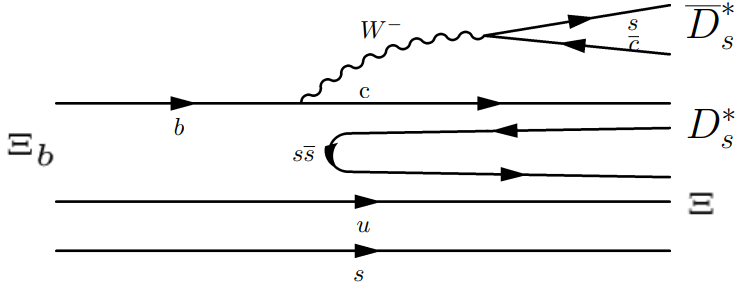
Figure 16: Microscopic quark level $\Xi_{b}\to\Xi~{}D_{s}^{*}~{}\bar{D}_{s}^{*}$ transition, through external emission.

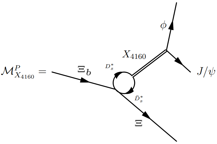
Figure 17: Mechanism for the $\Xi_{b}\to J/\psi~{}\phi~{}\Xi$ decay involving the $X(4160)$ resonance.

The dominant process for the $\Xi_{b}$ decay at the quark level proceeds via the external emission mechanism depicted in Fig. 16. Since the final state involves $J/\psi\,\phi$ pairs, the $D_{s}^{*}\,\bar{D}_{s}^{*}$ lines have to be connected to form a loop, as shown in Fig. 17, allowing multiple coupled channel interactions and generating dynamically the $X(4160)$, which then decays into $J/\psi$ and $\phi$. According to ref. Molina:2009ct the $X(4160)$ couples with maximum strength to the $D_{s}^{*}\,\bar{D}_{s}^{*}$ channel, but its coupling to the $J/\psi\,\phi$ channel is also significant, what also increase the dominance of the process depicted in Fig. 17. On the other hand, if we draw a diagram which would be responsible even for a direct $J/\psi\,\phi\Xi$ decay, at the microscopic quark level this reaction proceeds via the internal conversion process, shown in Fig. 18, which is strongly penalized by color factors color_fac and therefore it will be neglected in this work, similar to what was done in Ref. Magas:2020zuo ; Wang:2017mrt .

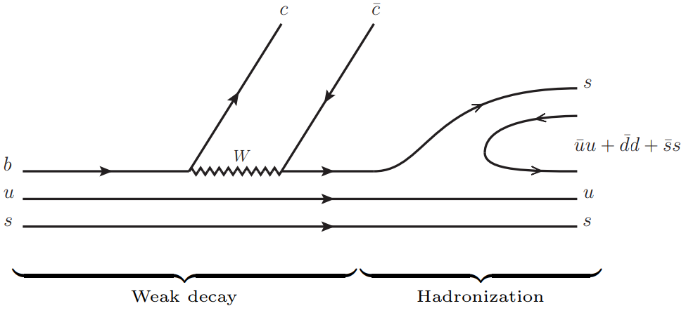
Figure 18: Microscopic quark level production of $J/\psi\ \phi\ \Lambda$ in the $\Lambda_{b}$ decay through internal conversion.

The amplitude of the dominant process (Fig. 17) can be written as:

$${\cal M}^{P}_{X_{4160}}=A(\vec{\epsilon}_{J/\psi}\times\vec{\epsilon}_{\phi})\cdot\vec{P}_{\Xi}G_{D_{s}^{*}\bar{D}_{s}^{*}}\frac{T_{D_{s}^{*}\bar{D}_{s}^{*},J/\psi\phi}}{g_{D_{s}^{*}\bar{D}_{s}^{*}}g_{J/\psi\phi}}.$$ (23)

The $A$ on the right side of the equation represents the strength of the $\Xi_{b}\to\Xi D_{s}^{*}~{}\bar{D}_{s}^{*}$ weak decay, shown in Fig. 16, which we are not going to study in details. This value can be taken as a constant due to the limited range of energies involved in the $\Xi_{b}\to\Xi~{}J/\psi~{}\phi$ decay as it is argued in Ref. Feijoo:2015cca . The $(\vec{\epsilon}_{J/\psi}\times\vec{\epsilon}_{\phi})\cdot\vec{P}_{\Xi}$ factor denotes the P-wave operator which is the minimum partial wave we need in the weak vertex to conserve the angular momentum, since the spins of $\Xi_{b}$ and $\Xi$ are $J=1/2$ while for the $X(4160)$ is $J=2$. Here $\vec{\epsilon}_{i}$ represents the polarization of the vector mesons in the $J/\psi~{}\phi$ rest frame and $\vec{P}_{\Xi}$ the tree-momentum of the $\Xi$ in the same frame. The factor $G_{D_{s}^{*}\bar{D}_{s}^{*}}$ indicates the contribution of the $D_{s}^{*}\bar{D}_{s}^{*}$ loop shown in Fig. 17 and the $T_{D_{s}^{*}\bar{D}_{s}^{*},J/\psi\phi}$ term is the coupled-channel unitarized amplitude for the $D_{s}^{*}\bar{D}_{s}^{*}\to J/\psi~{}\phi$ process. Note that we divide it by the corresponding couplings constants. This is done for a proper comparison with the $X(4140)$ term.

Now we will discuss the alternative way of our reaction via production of $X(4140)$, as it is shown in Fig. 19. The associated amplitude is

$${\cal M}^{P}_{X_{4140}}=\frac{B}{2M_{X(4140)}[M_{J/\psi\phi}-M_{X(4140)}+i\frac{\Gamma_{X(4140)}}{2}]},$$ (24)

where the $X(4140)$ is parameterised with a Breit-Wigner, where $M_{J/\psi\phi}$ is the invariant mass of the $J/\psi\phi$ system and $M_{X(4140)}$ and $\Gamma_{X(4140)}$ are the mass and width of $X(4140)$ resonance, respectively. A new constant, connected to the strength of the $\Xi_{b}\to\Xi~{}X(4140)$ weak decay, is $B$ and, since we want it to have the same units as $A$, we introduce a $2M_{X(4140)}$ factor in the denominator. In this process we do not need to have a P-vertex since the quantum number of the $X(4140)$ is $J=1$. Therefore the minimum partial wave needed to conserve the angular momentum is $L=0$.

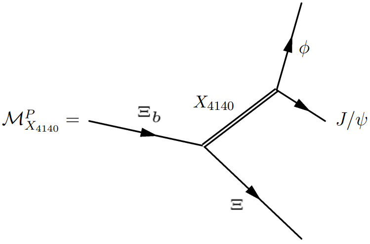
Figure 19: Mechanism for the $\Xi_{b}\to J/\psi~{}\phi~{}\Xi$ decay involving the $X(4140)$ resonance

We will not go into more detailed calculations, since the main aim of this work is to point out the possibility to use the $\Xi_{b}\to\Xi~{}J/\psi~{}\phi$ decay to study already discovered and potentially new exotic states and to encourage to the experimental collaborations to explore this reaction.

IV.3 Final state interaction

Once we discussed the generation of the $\Xi~{}J/\psi~{}\phi$ final state in $\Xi_{b}$ decay we want to focus on studying the final state interaction in the $\Xi~{}J/\psi$ and $\Xi~{}\phi$ channels. For the case of the final state interaction of $\Xi~{}J/\psi$ pair the $\Xi$ and $J/\psi$ legs from Fig. 17 and 19 have to be connected, forming a loop, which can dynamically generate the $S=-2$ pentaquark. The $\Xi~{}\phi$ final state interaction can produce excited $\Xi$ states and has to be studied in a similar way.

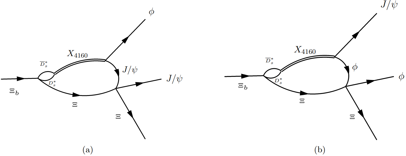
Figure 20: Final state interaction between $J/\psi~{}\Xi$ (a) and $\phi~{}\Xi$ (b) in the presence of the $X(4160)$ resonance.

The amplitude associated to the process with the final state interaction of the $J/\psi\Xi$ pair driven by the $\Xi_{b}$ decay via $X(4160)$ resonance is:

$${\cal M}^{J/\psi\Xi}_{X_{4160}}=A(\vec{\epsilon}_{J/\psi}\times\vec{\epsilon}_{\phi})\cdot\bigg{(}\frac{\vec{P}_{\Xi}-\vec{P}_{\phi}}{2}\bigg{)}T_{J/\psi\Xi,J/\psi\Xi}I^{J/\psi\Xi}_{X_{4160}},$$ (25)

which is associated to the diagram shown in Fig. 20(a), where the superscript denotes the final state interaction channel. This expression is derived in Appendix A, where the expression for the integral $I^{J/\psi\Xi}_{X_{4160}}$ is also given. We would like to remind the reader that for the reaction via $X(4160)$ the weak decay vertex has to be a P-wave one. Therefore the operator assigned to the the $\Xi_{b}\to D^{*}_{s}~{}\bar{D}^{*}_{s}~{}\Xi$ is proportional to the momentum of $\Xi$ and the loop integral (Fig. 20(a)) becomes a tree-vector. We evaluate this loop integral in the $J/\psi~{}\Xi$ rest frame, where the loop integral becomes proportional to $\frac{(\vec{P}_{\Xi}-\vec{P}_{\phi})}{2}$, with the scalar coefficient $I^{J/\psi\Xi}_{X_{4160}}$. The term $T_{J/\psi\Xi,J/\psi\Xi}$ captures the final state interaction contribution from $J/\psi~{}\Xi$, which in this work we will model using a Breit-Wigner form:

$$T_{J/\psi\Xi,J/\psi\Xi}=\frac{g_{J/\psi~{}\Xi}^{2}}{M_{J/\psi~{}\Xi}-M+i\frac{\Gamma}{2}},$$ (26)

were $g_{J/\psi~{}\Xi}$ is the coupling of the $S=-2$ pentaquark to the $J/\psi~{}\Xi$ channel. $M_{J/\psi~{}\Xi}$ denotes the invariant mass of the $J/\psi~{}\Xi$ system, and $M$ and $\Gamma$ denote the mass and the width of the $S=-2$ pentaquark. The values of $g_{J/\psi~{}\Xi}$, $M$ and $\Gamma$ will be obtained from the molecular model of a VB interacting discussed in section II.

For the final state interaction of the $\phi~{}\Xi$ pair we can repeat similar calculations and obtain (see Appendix A):

$${\cal M}^{\phi\Xi}_{X_{4160}}=A(\vec{\epsilon}_{J/\psi}\times\vec{\epsilon}_{\phi})\cdot\bigg{(}\frac{\vec{P}_{\Xi}+\vec{P}_{\phi}}{2}\bigg{)}T_{\phi\Xi,\phi\Xi}I^{\phi\Xi}_{X_{4160}},$$ (27)

where the $T_{\phi\Xi,\phi\Xi}$ amplitude is also taken as a Breit-Wigner form, as in Eq. (26), but in this case $M$ and $\Gamma$ are the experimental mass and width of the $\Xi(2500)$. Since we do not have any model which can give us the value of $g_{\phi\Xi}$, we will invert the problem and will study for which values of $g_{\phi\Xi}$ it is feasible to see this state using the $\Xi_{b}\to\Xi~{}J/\psi~{}\phi$ reaction.

Now we go to the final state interaction in the presence of the $X(4140)$ resonance. The corresponding diagrams are given in Figs. 21(a) and 21(b) and the associated analytical expressions are

$${\cal M}^{J/\psi\Xi}_{X_{4140}}=\tilde{B}T_{J/\psi\Xi,J/\psi\Xi}I^{J/\psi\Xi}_{X_{4140}},$$ (28)

$${\cal M}^{\phi\Xi}_{X_{4140}}=\tilde{B}T_{\phi\Xi,\phi\Xi}I^{\phi\Xi}_{X_{4140}}.$$ (29)

These expressions are explained in more detail in Appendix A. The terms $I^{J/\psi\Xi}_{X_{4140}}$ and $I^{\phi\Xi}_{X_{4140}}$ are scalar loop integral analogous to those in Eqs. (25) and (27).

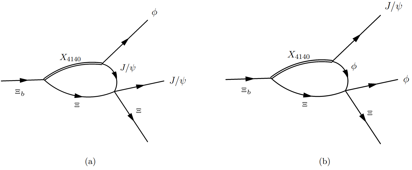
Figure 21: Final state interaction between $J/\psi~{}\Xi$ (a) and $\phi~{}\Xi$ (b) in the presence of the $X(4140)$ resonance.

IV.4 Full amplitude and decay rate

Now we proceed to combine the various terms to form the full invariant amplitude. Firstly we put together the $X(4140)$ terms into a ${\cal M}_{X_{4140}}$ amplitude, and similarly for $X(4160)$ terms,

$$B\,{\cal M}_{X_{4140}}={\cal M}^{P}_{X_{4140}}+{\cal M}^{J/\psi\Xi}_{X_{4140}}+{\cal M}^{\phi\Xi}_{X_{4140}},$$ (30)

$$A\,{\cal M}_{X_{4160}}={\cal M}^{P}_{X_{4160}}+{\cal M}^{J/\psi\Xi}_{X_{4160}}+{\cal M}^{\phi\Xi}_{X_{4160}},$$ (31)

where we wrote explicitly the primary decay strengths $A$ and $B$. And secondly, we mix these terms obtaining the full amplitude denoted as ${\cal M}$,

$$\overline{|{\cal M}|^{2}}=|A|^{2}\overline{{|\cal M}_{4160}|^{2}}+|B|^{2}\overline{{|\cal M}_{4140}|^{2}}$$

$$=|A|^{2}\Big{(}\overline{{|\cal M}_{4160}|^{2}}+\beta\,\overline{{|\cal M}_{4140}|^{2}}\Big{)},$$ (32)

where the bar represents the sum over polarizations and $\beta=|B|^{2}/|A|^{2}$. Note that, since the weak decay goes in P-wave for the $X(4160)$ contribution and in S-wave for the $X(4140)$ contribution, the cross term in $\overline{{|\cal M}_{4160}+{\cal M}_{4140}|^{2}}$ cancels as these two partial waves are orthogonal and do not interfere. It is also important to comment that, although the the overall factor $|A|^{2}$ is not known, it is not relevant for the shape of the obtained distributions. The form of the distributions, and not its absolute value, will be our main observable. We are exploring if the position of the peak and its width can be measured in several model situations. So our final results will be given in arbitrary units, therefore we will set $|A|^{2}=1$ from here to the end of this work:

$$\overline{|{\cal M}|^{2}}=\overline{{|\cal M}_{4160}|^{2}}+\beta\,\overline{{|\cal M}_{4140}|^{2}}\,.$$ (33)

The $\beta$ acts like a relative weight between the $X(4140)$ and $X(4160)$ contributions. In this work we will not calculate its value and we do not have any experimental result to compare it, so we take the value of $\beta$ from Ref. Wang:2017mrt to solve this issue. In this reference the authors study the interplay between $X(4160)$ and $X(4140)$ in the $B^{+}\to J/\psi~{}\phi~{}K^{+}$ decay. The mechanism involving the $X(4160)$ in this reaction is rather similar at the quark level to our diagram shown in Fig. 16, but without the spectator $s$ quark in the initial and final state. Hence the topology of the diagrams is similar also in the case of $X(4140)$. Therefore the $\beta$ value in our reaction may be similar as that in Ref. Wang:2017mrt , but we do not expect it to be the exactly the same, since the partial waves involved in their weak decay vertex are P-wave and D-wave for the $X(4140)$ and $X(4160)$ resonances respectively.

Finally, we explain how we deal with the sum over the polarizations appearing in Eq. (33). For the ${\cal M}_{X(4140)}$ amplitude this calculation is trivial and it only produces a constant, which can be reabsorbed into $\beta$, but for the ${\cal M}_{X(4160)}$ amplitude the calculation is more complicated adding cross term contributions. The full derivation is presented in Appendix B.

First of all, we introduce the following definitions:

$${\cal M}^{P}_{4160}=(\vec{\epsilon}_{J/\psi}\times\vec{\epsilon}_{\phi})\cdot\vec{P}_{\Xi}~{}\tilde{{\cal M}}^{P}_{4160},$$ (34)

$${\cal M}^{J/\psi\Xi}_{4160}=(\vec{\epsilon}_{J/\psi}\times\vec{\epsilon}_{\phi})\cdot\vec{K}_{2}~{}\tilde{{\cal M}}^{J/\psi\Xi}_{4160},$$ (35)

$${\cal M}^{\phi\Xi}_{4160}=(\vec{\epsilon}_{J/\psi}\times\vec{\epsilon}_{\phi})\cdot\vec{K}_{1}~{}\tilde{{\cal M}}^{\phi\Xi}_{4160},$$ (36)

where $\vec{K}_{1}\equiv(\vec{P}_{\Xi}+\vec{P}_{\phi})/2$ and $\vec{K}_{2}\equiv(\vec{P}_{\Xi}-\vec{P}_{\phi})/2$. Then, as it is shown in Appendix B, the sum over the polarizations leads to

$$\overline{|{\cal M}_{4160}|^{2}}= |\vec{P}_{\Xi}|^{2}|\tilde{{\cal M}}^{P}_{4160}|^{2}+$$

$$|\vec{K}_{2}|^{2}|\tilde{{\cal M}}^{J/\psi\Xi}_{4160}|^{2}+|\vec{K}_{1}|^{2}|\tilde{{\cal M}}^{\phi\Xi}_{4160}|^{2}$$

$$+2\vec{P}_{\Xi}\cdot\vec{K}_{2}\Re(\tilde{{\cal M}}^{P}_{4160}\tilde{{\cal M}}^{*J/\psi\Xi}_{4160})$$

$$+2\vec{P}_{\Xi}\cdot\vec{K}_{1}\Re(\tilde{{\cal M}}^{P}_{4160}\tilde{{\cal M}}^{*\phi\Xi}_{4160})$$

$$+2\vec{K}_{1}\cdot\vec{K}_{2}\Re(\tilde{{\cal M}}^{J/\psi}_{4160}\tilde{{\cal M}}^{*\phi\Xi}_{4160}),$$

where $\Re$ is the real part of the complex argument.

Finally, the double differential cross-section for the $\Xi_{b}\to J/\Psi\phi\Xi$ decay process reads rocamai :

$$\frac{d^{2}\Gamma}{dM_{\phi\Xi}dM_{J/\psi\Xi}}=$$ (38)

$$\frac{1}{{(2\pi)}^{3}}\frac{4M_{\Xi_{b}}M_{\Xi}}{32M_{\Xi_{b}}^{3}}\,\overline{|{\cal M(M_{\phi\Xi},M_{J/\psi\Xi})}|^{2}}\,2M_{\phi\Xi}\,2M_{J/\psi\Xi}\,,$$

where $\mathcal{M}$ is given by eq. (33). As an example, we wrote in eq. (IV.4) cross section in function of $M_{\phi\Xi}$ and $M_{J/\psi\Xi}$ invariant masses, but we can write similar expression for any other combination of the two particle invariant masses of the $J/\Psi\phi\Xi$ final state (since out of three possible combination only two are independent).

Then, for example, fixing the invariant mass $M_{J/\psi\Xi}$, one can integrate over $M_{\phi\Xi}$ in order to obtain $d\Gamma/dM_{J/\psi\Xi}$. In this case, the limits are given by:

$$\left(M_{\phi\Xi}^{2}\right)_{\rm max} = {\left(E^{*}_{\Xi}+E^{*}_{\phi}\right)}^{2}$$ (39)

$$-{\left(\sqrt{{E^{*}_{\Xi}}^{2}-M^{2}_{\Xi}}-\sqrt{{E^{*}_{\phi}}^{2}-m^{2}_{\phi}}\right)}^{2}$$

and

$$\left(M_{\phi\Xi}^{2}\right)_{\rm min} = {\left(E^{*}_{\Xi}+E^{*}_{\phi}\right)}^{2}$$ (40)

$$-{\left(\sqrt{{E^{*}_{\Xi}}^{2}-M^{2}_{\Xi}}+\sqrt{{E^{*}_{\phi}}^{2}-m^{2}_{\phi}}\right)}^{2}\,$$

where

$$E^{*}_{\Xi}=\frac{M_{J/\psi\Xi}^{2}-m_{J/\psi}^{2}+M^{2}_{\Xi}}{2M_{J/\psi\Xi}}\ ,$$ (41)

$$E^{*}_{\phi}=\frac{M_{\Xi_{b}}^{2}-M_{J/\psi\Xi}^{2}-m^{2}_{\phi}}{2M_{J/\psi\Xi}}\ .$$ (42)

Similar formulas are obtained when fixing the invariant mass $M_{\phi\Xi}$ and integrating over $M_{J/\psi\Xi}$ to obtain $d\Gamma/dM_{\phi\Xi}$.

V Exotic hadrons in $\Xi_{b}\to J/\Psi\phi\Xi$ decay

V.1 The $J/\psi~{}\phi$ mass distribution

We start studying the $J/\psi~{}\phi$ mass distribution, which will allow us to see the $X(4140)/X(4160)$ interplay. We consider two possibles models: in the first one, which is based in the latest experimental results (Refs. LHCb:2016axx ; LHCb:2016nsl ), we assume existence of only one broad $X(4140)$ resonance with a pole position of $M_{R}=4146.5~{}{\rm MeV}$ and a width of $\Gamma=83~{}{\rm MeV}$; while the second model assumes the existence of a narrow $X(4140)$ plus a wide $X(4160)$ resonance, based on earlier experimental results Wu:2010vk ; Hofmann:2005sw ; Yuan:2012wz ; Xiao:2013yca ; Garcia-Recio:2013gaa and a recent theoretical model Wang:2017mrt .

We start with the model with a wide $X(4140)$. The corresponding results are shown in Fig. 22, where we can see the $J/\psi~{}\phi$ invariant mass distribution for the tree level calculations (Fig. 19) and the corresponding spectrum when we also take into account the FSI (Figs. 21). As we can see, the effect of the FSI is rather small. This will be also true for the model with two $X$ resonances, so in this section we will further present only the results that include the FSI.

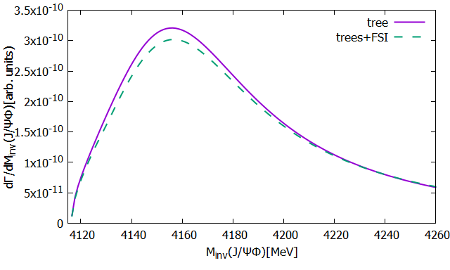
Figure 22: The $J/\psi~{}\phi$ mass spectrum computed using one wide $X(4140)$ resonance. The green line corresponds to tree level calculations only, while the purple one also includes the FSI effects.

Once seen the results for the one resonance model we are going to discuss the results generated with two resonances, where similarly to the results of Ref. Magas:2020zuo we adjust the parameter $\beta$ to a value which generates two $X$ resonances of a similar strength. The $X(4140)$ resonance has a mass of $M_{R}=4132~{}{\rm MeV}$ and a width of $\Gamma=19~{}{\rm MeV}$, while the $X(4160)$ can be generated as $D^{*}_{s}\bar{D}^{*}_{s}$ molecule, as we explained in Section IV.2. The corresponding model contains a loop-function that diverges and must be regularised. In Ref. Molina:2009ct this loop function is regularised using a dimensional regularisation method but, as we proved earlier, such a scheme can produce fake poles, so in this work we use the cut-off regularisation method with $\Lambda=650~{}{\rm MeV}$, which reproduces the results obtained using the dimensional regularisation from Molina:2009ct .

The $J/\psi~{}\phi$ invariant mass distribution for two $X$ resonances can be seen in Fig. 23, where we can see a narrow $X(4140)$ peak at $4132~{}{\rm MeV}$ and a rather wide $X(4160)$ peak. Note that the $X(4160)$ also produces a cusp around $4224~{}{\rm MeV}$, which corresponds to the $D^{*}_{s}\bar{D}^{*}_{s}$ threshold. As it is mentioned in Ref. Magas:2020zuo , if this cusp is experimentally detected it would strongly suggest a molecular interpretation of $X(4160)$, as well as the existence of a narrow $X(4140)$ and a wide $X(4160)$ resonance in this energy region.

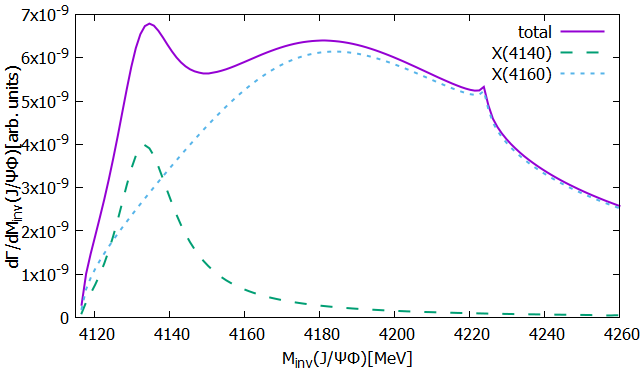
Figure 23: The purple line represents the $J/\psi~{}\phi$ mass spectrum generated using two resonance model. The green and the blue lines show the individual contributions from $X(4140)$ and $X(4160)$, respectively.

For the results presented in Fig. 23 the parameter $\beta$, Eq. 33, is taken as $\beta=\beta_{0}/2.6$, where $\beta_{0}$ is the value taken in Ref. Wang:2017mrt . We would also like to analyse the sensibility of the obtained distribution with respect to the parameter $\beta$ and, for this purpose, we generated similar spectra for different values of $\beta$ and present these in Fig. 24. As it can be expected from eq. (33), changing the values of $\beta$ mainly affects the height of the $X(4140)$ peak.

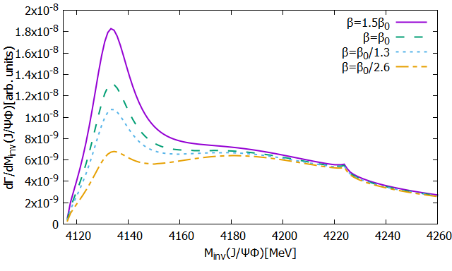
Figure 24: The solid lines represent the $J/\psi~{}\phi$ mass spectrum generated using the $X(4140)$ and the $X(4160)$ resonances for different values of the weight factor $\beta$, which controls the relative contributions of the two resonances; $\beta_{0}$ is the value of $\beta$ given in Ref. Wang:2017mrt

V.2 The $J/\psi~{}\Xi$ mass distribution

Now we discuss the results for the $J/\psi~{}\Xi$ mass distribution, which is the channel where we expect to see the signature of the $S=-2$ pentaquark. The properties of these pentaquark, dynamically generated by our model, are presented in Tab. 7. This state has a mass $M_{R}=4633.38~{}{\rm MeV}$ and a width $\Gamma_{R}=79.58~{}{\rm MeV}$, and couples rather strongly to the $J/\psi~{}\Xi$ channel, with a coupling constant value of $g_{J/\phi\Xi}=-1.62+0.38i$. We will take these values for the pole position and coupling as the nominal ones and we will vary them within a reasonable range to explore the sensitivity of our results with respect to the pentaquark parameters. We also will study the effect of narrow state in the $J/\psi~{}\Xi$ channel by using the parameters obtained in ref. Roca:2024nsi , where the state has a mass $M_{R}=4617~{}{\rm MeV}$, a width $\Gamma_{R}=12~{}{\rm MeV}$ and the coupling constant to the $J/\psi~{}\Xi$ channel is $g_{J/\phi\Xi}=0.66+0.0i$.

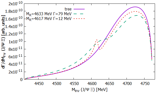
Figure 25: The $J/\psi~{}\Xi$ spectrum, where the purple line corresponds to the tree level diagram and the green and red one is obtained also taking into account the final state interactions that generates the $S=-2$ pentaquark which has $M_{R}=4633~{}MeV$ and $\Gamma=79~{}MeV$ or $M_{R}=4617~{}MeV$ and $\Gamma=12~{}MeV$ respectively.

Proceeding in a similar manner as in the previous section, we start showing our results computed with one wide $X(4140)$ resonance. In Fig. 25 we can see the $J/\psi~{}\Xi$ spectrum, where the solid line is obtained using only the tree-level diagram, while the dashed lines include also the FSI effects. In these latter curves we should see the signal of the $S=-2$ pentaquark, generated in the $J/\psi~{}\Xi$ interaction. First of all, as can be seen in Fig. 25, the background shows itself a peak structure around $4730~{}{\rm MeV}$. The pentaquark, in both studied cases, interferes with the background positively and has an important effect on the spectrum due to its strong coupling to the $J/\psi~{}\Xi$ channel. The presence of the pentaquark in FSI manifest itself as the appearance of a bump around the nominal pentaquark mass of $4633~{}{\rm MeV}$ in the case of the wide resonances from our model. That bump is not very prominent, however it seems to be detectable. Meanwhile for the case we have a narrow pentaquark from Roca:2024nsi the peak that is formed due to its existence is not much higher than the bump and also perfectly detectable. The explanation for this phenomenon is rather straightforward: narrow pentaquark is much sharper and at the first glance seems to be easier detectable, however it is narrower, because its coupling to the lowest open channel $J/\psi\Xi$ is smaller, and thus the amplitude $T_{J/\psi\Xi,J/\psi\Xi}\sim g_{J/\psi\Xi}^{2}$ is also smaller, producing at the end of the day approximately the same signal to noise ration.

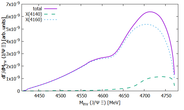
Figure 26: The purple line represents the $J/\psi~{}\Xi$ spectrum computed with a narrow $X(4140)$ plus a $X(4160)$, while the green and the blue ones show the individual contribution from the $X(4140)$ and the $X(4160),$ respectively.

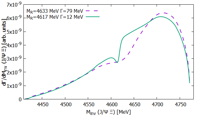
Figure 27: The purple line dashed represents the $J/\psi~{}\Xi$ spectrum computed with a narrow $X(4140)$ plus a $X(4160)$ having a resonance with $M_{R}=4633~{}MeV$ and $\Gamma=79~{}MeV$, while the green and the blue ones show similar results but having a resonance with, respectively $M_{R}=4617~{}MeV$ and $\Gamma=12~{}MeV$.

Let’s now consider the calculation with a narrow $X(4140)$ and a wide $X(4160)$ resonances. The results (with FSI) can be seen in Fig. 26, where the green and the blue curves show the individual contributions of the $X(4140)$ and the $X(4160)$ resonances respectively, while the purple solid curve is the sum of both contributions. Note that the $X(4160)$ contribution is dominant with respect to that of the $X(4140)$. It is also important to see that, in contrast to the previous case, the signal of the pentaquark interferes negatively with the background. This can be seen more clearly in Fig. 27, where we compare the contributions from wide and narrow pentaquarks. Again we see that the presence of $P_{css}$ is well detectable in ambos cases, and that both produce approximately the same signal to noise ration. For the further studies we will concentrate on wider pentaquark produced by our model, as discussed in section III.2.

In Fig. 28 where we compare the contribution from one and two $X$ resonance models with FSI, varying the mass of the wide pentaquark and its coupling to the $J/\psi~{}\Xi$ channel. We do that since we know there can exist some theoretical uncertainties, so we modify the pentaquark pole position by $\pm 50~{}{\rm MeV}$ and we allow for a $20\%$ of variation of the coupling of the pentaquark to the channel $J/\psi~{}\Xi$. The results presented in Fig. 28 clearly show that the presence of the double strangeness pentaquark is experimentally detectable in all cases. Actually, in the case of one wide $X(4140)$ this task seems to be much simpler. And certainly the experimental measurement of the $J/\psi~{}\Xi$ invariant mass spectrum from the $\Xi_{b}\to\Xi~{}J/\psi~{}\phi$ decay would also allow one to distinguish between one wide $X(4140)$ or two $X$ models.

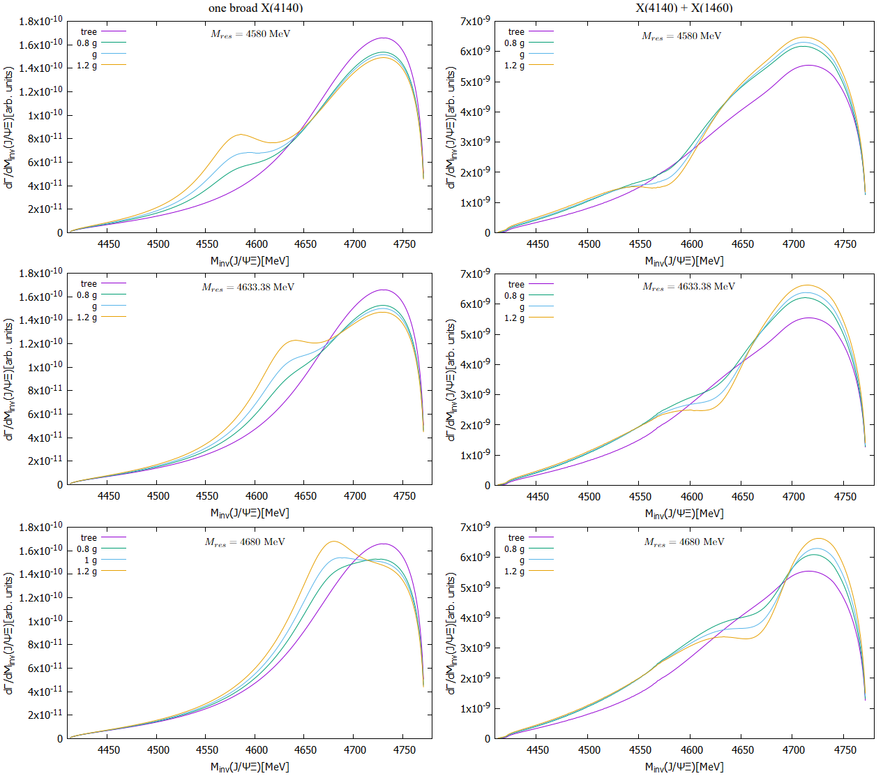
Figure 28: $J/\psi~{}\Xi$ spectrum computed with one broad $X(4140)$ resonance (left panels) or with a narrow $X(4140)$ plus a $X(4160)$ state (right panels) with different values of the $g_{J/\psi\Xi}$ coupling and different pole positions for the resonance [$4580~{}{\rm MeV}$ (top), $4663.38~{}{\rm MeV}$ (middle) and $4680~{}{\rm MeV}$ (bottom)]

V.3 The $\phi~{}\Xi$ mass distribution

Finally, we present the results for the $\phi~{}\Xi$ invariant mass distribution where we expect to see the signal of the $\Xi(2500)$. This state appears in the PDG PDG as a one-star state, with a mass of $M_{\Xi(2500)}=2500~{}{\rm MeV}$ and there exist two experimental groups that reported different values for its width, namely $150~{}{\rm MeV}$ Alitti:1969rb and $50~{}{\rm MeV}$ Aachen-Berlin-CERN-London-Vienna:1969bau . Based on this information we decided to generate the spectrum for tree different cases, $\Gamma=50,~{}100,~{}150~{}{\rm MeV}$. We do not know either which is the coupling constant of this state to the $\phi~{}\Xi$ channel, therefore we explore a range of values for this coupling, which would allow us to see the signal of the $\Xi(2500)$ in generated the spectrum.

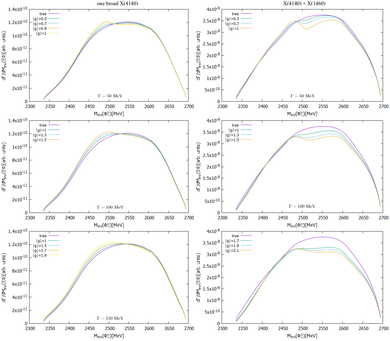
Figure 29: The $\phi~{}\Xi$ spectrum computed with one broad $X(4140)$ resonance (left panels) or with narrow $X(4140)$ plus a $X(4160)$ states (right panels) with different values for the coupling of the $\Xi(2500)$ to the $\phi~{}\Xi$ channel, and different widths of the resonance [$50~{}{\rm MeV}$ (top), $100~{}{\rm MeV}$ (middle) and $150~{}{\rm MeV}$ (bottom)]

The corresponding results are the presented in Fig. 29. The value of the coupling constant, needed to generate a significant interference with the background, as we could expect, is larger if the state has a larger width. We can see that if $\Gamma=50~{}{\rm MeV}$ then the minimum absolute value of the coupling is around $0.7$, while for a $\Xi(2500)$ with $\Gamma=150~{}{\rm MeV}$ this value is around $1.7-1.9$. Similarly to the previous case, the interference of the resonance with the background is positive for the case of one wide $X(4140)$ resonance, while for the case of a narrow $X(4140)$ and wide $X(4160)$ resonances the interference is negative. Thus, we see that studying this spectrum would also be very interesting if the coupling of the $\Xi(2500)$ to the $\phi~{}\Xi$ states is large enough.

VI Conclusions

The discovery in the last years of many exotic hadrons not fitting into the conventional quark composition model, has converted this topic into an important field of research. Motivated by this fact, in the present work we studied some resonances that could be interpreted as quasi-bound states of an interacting meson-baryon pair in the strangeness $-2$ and isospin $1/2$ sector, employing effective Lagrangians for describing the exchange of a vector meson in the t-channel. We also proposed a decay process $(\Xi_{b}\to\Xi~{}J/\psi~{}\phi)$ suitable to detect some of those exotic hadrons in all two-particle channels.

First of all, in this work we find two poles, which can be associated to the $\Xi(1620)$ and $\Xi(1690)$ resonances from PDG PDG , in the scattering amplitude of the interaction of pseudoscalar mesons with baryons in the light-channel sector. By modifying some parameters in a reasonable range we can reproduce the experimental masses of the $\Xi(1620)$ and $\Xi(1690)$, producing two states at $1600~{}{\rm MeV}$ and $1685.40~{}{\rm MeV}$. With this result we can conclude that the $\Xi(1620)$ and the $\Xi(1690)$ may have a meson-baryon molecular origin. The $\Xi(1620)$ would have an important $\pi\Xi$ component, around $50\%$, with a $20\%$ mixture of $\bar{K}\Lambda$. The $\Xi(1690)$ would be mainly a $\bar{K}\Sigma$ molecule with a small component $(2\%)$ of $\eta\Xi$. Both of these resonances have well defined spin-parity $(J^{\pi}=\frac{1}{2}^{-})$, and thus a measurement of the spin-parity of these states could confirm or refute this hypothesis.

For the light-channel sector of the VB interaction we can also find two resonances in the scattering amplitude, which could be associated with two states listed in the PDG, namely the $\Xi(1820)$ and $\Xi(1950)$ PDG . Similarly to what we did in the PB section, by modifying some parameters we can bring the positions of these two states closer to their experimental mass, but the theoretical widths are much smaller than the experimental ones. This might be solved by allowing the coupling between the vector mesons with the pseudoscalar mesons, and thus opening decays to lighter channels and correspondingly increasing the width of the dynamically generated states. If the present interpretation is assumed to represent the nature of these states, we could understand the $\Xi(1820)$ as a mixture of $\phi\Xi$ $(33\%)$ and $\bar{K}^{*}\Lambda$ $(13\%)$ components, while the $\Xi(1950)$ would be a mixture of $\bar{K}^{*}\Sigma$ $(50\%)$, $\omega\Xi$ $(10\%)$ and $\phi\Xi$ $(10\%)$ ones. Note that these states are degenerate in spin-parity and form a $J^{\pi}=\frac{1}{2}^{-}$, $J^{\pi}=\frac{3}{2}^{-}$ doublet. This would be compatible with the observed quantum numbers of the $\Xi(1820)$, which are $J^{\pi}=\frac{3}{2}^{-}$.

Alternatively our model allows to generate these two resonances in the region of the $\Xi(1950)$, producing an apparent wide resonance. This is a possibility mentioned in the PDG, where it is said that the $\Xi(1950)$ may in fact be more than one $\Xi$ state.

Furthermore, the results for the heavy channels are quite encouraging, as they point towards the existence of doubly strangeness pentaquarks with hidden charm, which can be generated thanks to the coupled-channel structure of our model. The absence in this sector of a long range interaction mediated by pion-exchange also makes the search for these states specially interesting. If they do exist, their interpretation as molecules would require a change of paradigm, since they could only be bound through heavier-meson exchange models as the one employed in this work, see ref. Marse-Valera:2022khy for more details.

Indeed, in the pseudoscalar meson baryon interaction sector we can generate one hidden charm $S=-2$ baryon with $M=4493~{}{\rm MeV}$ and $\Gamma=73~{}{\rm MeV}$, which can be interpret as a $\bar{D}\Omega_{c}$ molecule, and the quantum numbers of this state would be $J^{\pi}=\frac{1}{2}^{-}$. In the vector meson baryon interaction sector we can also generate one state with $M=4633~{}{\rm MeV}$ and $\Gamma=79~{}{\rm MeV}$ and, similarly to the previous case, this state can be understood as a $\bar{D}^{*}\Omega_{c}$ molecule which would be degenerate in spin-parity forming a $J^{\pi}=\frac{1}{2}^{-}$, $J^{\pi}=\frac{3}{2}^{-}$ doublet.

The similar model of Ref. Roca:2024nsi also find such states, practically at the same mass, but with much narrower width. In the further study, Ref. Oset:2024fbk , the authors suggest the $\Xi_{b}^{0}\to\eta\eta_{c}\Xi^{0}$ and $\Omega_{b}^{-}\to K^{-}\eta_{c}\Xi^{0}$ decays in order to observe the $P_{css}$ with $I(J^{P})=\frac{1}{2}(\frac{1}{2}^{-})$ generated via pseudoscalar-baryon interaction. In contrast, in the present manuscript we have concentrated at the possibility to detect potential $P_{css}$ state generated in VB interaction in $\Xi_{b}\to\Xi~{}J/\psi~{}\phi$ decay.

Another motivation to study the $\Xi_{b}\to\Xi~{}J/\psi~{}\phi$ decay came form the Dalitz plots of Fig. 15, which proved the potential possibility to study several exotic states that may be detected in all three two-body invariant mass spectra. Similarly to what is done in Magas:2020zuo , we develop two different models for the interpretation of the $X(4140)$ and $X(4160)$ resonances. The first model considers that there only exists one wide $X(4140)$ state while the other claims the existence of a narrow $X(4140)$ resonance plus a $X(4160)$ one. Consequently in the $J/\psi~{}\phi$ mass spectrum, due to the nature of the $X(4160)$ as a $D^{*}_{s}\bar{D}_{s}^{*}$ Molina:2009ct bound system, there appears a cusp near the threshold of this channel $(4224~{}{\rm MeV})$. Therefore, if this cusp is detected, it would be a clear signal that the two-resonances model is the one that represents the nature of the $X$ resonances, and also that the $X(4160)$ is a molecular state.

The $X(4274)$, $X(4350)$ and the $X(4500)$ resonances may also leave a signal at higher $J/\psi$ invariant masses in the $\Xi_{b}\to\Xi~{}J/\psi~{}\phi$ decay, but in this work these states where not included as we do not have a theoretical model that generates them.

In the $J/\psi~{}\Xi$ spectrum, we studied the possibility of detecting the doubly strange pentaquark with hidden charm, which we introduce as a Breit-Wigner using the parameters obtained from the coupled channel approach developed in this work in section III.2. This permits us to keep the model simple and do variations on the parameters easily. The results are very promising, since if the mass of this state lies in the region $4580-4680~{}{\rm MeV}$ it has a good chance to be experimentally detected. We have also shown that in the case of a single wide $X(4140)$ model the pentaquark signal interferes positively with the background, while for the two $X$ model this interference is negative. This potentially allows one to differentiate between these two situations once the corresponding spectrum will be measured.

Finally, we also studied the $\phi~{}\Xi$ spectrum, where we explored the possibility to detect the $\Xi(2500)$. For this resonance there exists a discussion about whether its width is $50~{}{\rm MeV}$ or $150~{}{\rm MeV}$ PDG , so we studied these two possibilities plus an intermediate case of $\Gamma=100~{}{\rm MeV}$. Our results show that, if the resonance has a narrow width of $50~{}{\rm MeV}$, its signal in the spectrum has high chances to be detected even with small coupling $(g_{\phi\Xi}\sim 0.7-0.9)$, whereas if $\Gamma=100~{}{\rm MeV}$ the coupling should be bigger than $g_{\phi\Xi}=1.3$, and in the case $\Gamma=150~{}{\rm MeV}$ the value of the coupling has to be bigger than $g_{\phi\Xi}=1.9$ in order to produce a significant signal above the background.

Appendix A Appendix A: Double loop integral

In our discussion of the $\Xi_{b}\to\Xi~{}J/\psi~{}\phi$ decay we gave the expression for two final state interaction amplitudes ${\cal M}_{4160}^{J/\psi\Xi}$, and ${\cal M}_{4160}^{\phi\Xi}$ which involve a loop integral that is a 3-vector. In this appendix we demonstrate how we arrive to eqs. (25) and (27). Similarly, we will derive the expressions for the ${\cal M}_{4140}^{J/\psi\Xi}$ and ${\cal M}_{4140}^{\phi\Xi}$ amplitudes.

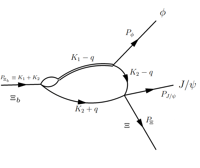
Figure 30: Feynman diagram associated to the ${\cal M}_{4160}^{J/\psi\Xi}$ amplitude, where we show the corresponding momenta for all the particle lines.

In Fig. 30 we can see the the diagram associated to the ${\cal M}_{4160}^{J/\psi\Xi}$, where the momenta of each particle is shown. From this diagram we can write the full expression of the ${\cal M}_{4160}^{J/\psi\Xi}$ amplitude, being:

$${\cal M}_{4160}^{J/\psi\Xi}=iT_{J/\psi\Xi,J/\psi\Xi}\int\frac{d^{4}q}{(2\pi)^{4}}G_{D_{s}^{*}\bar{D}_{s}^{*}}$$

$$\frac{(\vec{\epsilon}_{J/\psi}\times\vec{\epsilon}_{\phi})\cdot(\vec{K}_{2}+\vec{q})}{(K_{1}-q)^{2}-M_{X}^{2}+iM_{X}\Gamma_{X}}$$

$$\frac{1}{(K_{2}-q)^{2}-M_{J/\psi}^{2}+i\epsilon}$$

$$\frac{2M_{\Xi}}{(K_{2}+q)^{2}-M_{\Xi}^{2}+i\epsilon},$$ (43)

where we have defined $K_{1}=(P_{\Xi}+P_{\phi})/2$ and $K_{2}=(P_{\Xi}-P_{\phi})/2$ (and correspondingly $K_{1}+K_{2}=P_{\Xi}$ and $K_{1}-K_{2}=P_{\phi}$). $T_{J/\psi\Xi,J/\psi\Xi}$ denotes the scattering amplitude for the corresponding channels, which we introduce as a Breit-Wigner with the $S=-2$ pentaquark parameters. As it is discussed in section IV.3 the $J/\psi$ $\phi$ interaction has to be in P-wave what leads to appearance of the vector product of the corresponding polarization vectors. Finally, the three propagators are the ones corresponding to the three internal lines for the $J/\psi$, $\Xi$ and $X(4160)$ resonances. From this expression we can separate the $q^{0}$ component and rearrange some terms in order simplify it, obtaining that

$${\cal M}_{4160}^{J/\psi\Xi}=iT_{J/\psi\Xi,J/\psi\Xi}(\vec{\epsilon}_{J/\psi}\times\vec{\epsilon}_{\phi})\int\frac{d^{3}q}{(2\pi)^{3}}(\vec{K}_{2}+\vec{q})$$

$$\int\frac{dq^{0}}{2\pi}\frac{G_{D_{s}^{*}\bar{D}_{s}^{*}}}{(K_{1}^{0}-q^{0})^{2}-\omega_{X}^{2}+iM_{X}\Gamma_{X}}$$

$$\frac{1}{(K_{2}^{0}-q^{0})^{2}-\omega_{J/\psi}^{2}+i\epsilon}\frac{2M_{\Xi}}{(K_{2}^{0}+q^{0})^{2}-\omega_{\Xi}^{2}+i\epsilon},$$

where $\omega_{X}^{2}=M_{X}^{2}+(\vec{K}_{1}-\vec{q})^{2}$, $\omega_{J/\psi}^{2}=M_{J/\psi}^{2}+(\vec{K}_{2}-\vec{q})^{2}$ and $\omega_{\Xi}^{2}=M_{\Xi}^{2}+(\vec{K}_{2}+\vec{q})^{2}$. If we take a non relativistic limit this expression can be written like this,

$${\cal M}_{4160}^{J/\psi\Xi}=iT_{J/\psi\Xi,J/\psi\Xi}(\vec{\epsilon}_{J/\psi}\times\vec{\epsilon}_{\phi})\int\frac{d^{3}q}{(2\pi)^{3}}(\vec{K}_{2}+\vec{q})$$

$$\int\frac{dq^{0}}{2\pi}\frac{G_{D_{s}^{*}\bar{D}_{s}^{*}}}{2\omega_{X}[K_{1}^{0}-q^{0}-\omega_{X}+i\frac{\Gamma_{X}}{2}}$$

$$\frac{1}{2\omega_{J/\psi}[K_{2}^{0}-q^{0}-\omega_{J/\psi}+i\epsilon]}\frac{M_{\Xi}}{\omega_{\Xi}[K_{2}^{0}+q^{0}-\omega_{\Xi}+i\epsilon]}.$$

From this expression we can now clearly see where are the poles of this integral, which are

$$q^{0}=K_{1}^{0}-\omega_{X}+i\frac{\Gamma}{2} \rightarrow {\rm Resonance},$$ (46)

$$q^{0}=K_{2}^{0}-\omega_{J/\psi}+i\epsilon \rightarrow {\rm J/\psi~{}propagator},$$ (47)

$$q^{0}=-K_{2}^{0}+\omega_{\Xi}-i\epsilon \rightarrow {\rm\Xi~{}propagator}.$$ (48)

Since we have two poles above the real axis and one below, we compute the integral using the contour integration method choosing to close the contour in the lower half plane. Thus we only pick the $\Xi$ propagator pole, finding

$${\cal M}_{4160}^{J/\psi\Xi}=T_{J/\psi\Xi,J/\psi\Xi}(\vec{\epsilon}_{J/\psi}\times\vec{\epsilon}_{\phi})$$

$$\int\frac{d^{3}q}{(2\pi)^{3}}\frac{(\vec{K}_{2}+\vec{q})G_{D_{s}^{*}\bar{D}_{s}^{*}}}{2\omega_{X}[K_{1}^{0}+K_{2}^{0}-\omega_{\Xi}-\omega_{X}+i\frac{\Gamma_{X}}{2}}$$

$$\frac{1}{2\omega_{J/\psi}[2K_{2}^{0}-\omega_{\Xi}-\omega_{J/\psi}+i\epsilon]}\frac{M_{\Xi}}{\omega_{\Xi}}.$$ (49)

To compute this integral we work in the Jackson frame (the $J/\psi$ $\phi$ rest frame), where the $\vec{K}_{1}$ and $\vec{K}_{2}$ are almost equal since, $P_{\phi}$ is small. So we can can replace $\vec{K}_{1}$ with $\vec{K}_{2}$, and thus now the integral only depends on $\vec{K}_{2}$. So we can take the integral to be proportional to this vector, giving us

$${\cal M}_{4160}^{J/\psi\Xi}=T_{J/\psi\Xi,J/\psi\Xi}(\vec{\epsilon}_{J/\psi}\times\vec{\epsilon}_{\phi})\vec{K}_{2}I^{J/\psi\Xi}_{X(4160)},$$ (50)

with,

$$I^{J/\psi\Xi}_{X(4160)}=\int\frac{d^{3}q}{(2\pi)^{3}}\frac{\vec{K}_{2}\cdot\vec{q}~{}G_{D_{s}^{*}\bar{D}_{s}^{*}}}{2\omega_{X}[K_{1}^{0}+K_{2}^{0}-\omega_{\Xi}-\omega_{X}+i\frac{\Gamma_{X}}{2}]}$$

$$\frac{1}{|\vec{K}_{2}|^{2}}\frac{1}{2\omega_{J/\psi}[2K_{2}^{0}-\omega_{\Xi}-\omega_{J/\psi}+i\epsilon]}\frac{M_{\Xi}}{\omega_{\Xi}},$$

where we made the shift $\vec{q}\to\vec{q}+\vec{K}_{2}$, and $\omega_{X}=M_{X}^{2}+(2\vec{K}_{2}-\vec{q})^{2}$, $\omega_{J/\psi}=M_{J/\psi}^{2}+(2\vec{K}_{2}-\vec{q})^{2}$ and $\omega_{\Xi}=M_{\Xi}^{2}+\vec{q}^{2}$.

Once we have ${\cal M}_{4160}^{J/\psi\Xi}$, to evaluate the ${\cal M}_{4160}^{\phi\Xi}$ is rather straightforward, as we only need to change $J/\psi$ to $\phi$ and vice versa. In the Jackson frame this is equal to the interchange of $\vec{K}_{2}$ and $\vec{K}_{1}$, leading us to

$${\cal M}_{4160}^{\phi\Xi}=T_{\phi\Xi,\phi\Xi}(\vec{\epsilon}_{J/\psi}\times\vec{\epsilon}_{\phi})\vec{K}_{1}I^{\phi\Xi}_{X(4160)},$$ (52)

with,

$$I^{\phi\Xi}_{X(4160)}=\int\frac{d^{3}q}{(2\pi)^{3}}\frac{\vec{K}_{1}\cdot\vec{q}~{}G_{D_{s}^{*}\bar{D}_{s}^{*}}}{2\omega_{X}[K_{1}^{0}+K_{2}^{0}-\omega_{\Xi}-\omega_{X}+i\frac{\Gamma_{X}}{2}]}$$

$$\frac{1}{|\vec{K}_{1}|^{2}}\frac{1}{2\omega_{\phi}[2K_{1}^{0}-\omega_{\Xi}-\omega_{\phi}+i\epsilon]}\frac{M_{\Xi}}{\omega_{\Xi}},$$

where $\omega_{X}=M_{X}^{2}+(2\vec{K}_{1}-\vec{q})^{2}$, $\omega_{\phi}=M_{\phi}^{2}+(2\vec{K}_{1}-\vec{q})^{2}$ and $\omega_{\Xi}=M_{\Xi}^{2}+\vec{q}^{2}$.

Finally we can also derive the expressions for ${\cal M}_{4140}^{J/\psi\Xi}$, and ${\cal M}_{4140}^{\phi\Xi}$ proceeding in an analogous way with the difference that now we do not have the $G_{D^{*}_{s}\bar{D}^{*}_{s}}$ loop-function and all interactions are in S-wave, and consequently these amplitudes are scalars.

$${\cal M}_{4140}^{J/\psi\Xi}=T_{J/\psi\Xi,J/\psi\Xi}I^{J/\psi\Xi}_{X(4140)},$$ (54)

with,

$$I^{J/\psi\Xi}_{X(4140)}=\int\frac{d^{3}q}{(2\pi)^{3}}\frac{1}{2\omega_{X}[K_{1}^{0}+K_{2}^{0}-\omega_{\Xi}-\omega_{X}+i\frac{\Gamma_{X}}{2}]}$$

$$\frac{1}{2\omega_{J/\psi}[2K_{2}^{0}-\omega_{\Xi}-\omega_{J/\psi}+i\epsilon]}\frac{M_{\Xi}}{\omega_{\Xi}},$$

where $\omega_{X}=M_{X}^{2}+(2\vec{K}_{2}-\vec{q})^{2}$, $\omega_{J/\psi}=M_{J/\psi}^{2}+(2\vec{K}_{2}-\vec{q})^{2}$ and $\omega_{\Xi}=M_{\Xi}^{2}+\vec{q}^{2}$, and

$${\cal M}_{4140}^{\phi\Xi}=T_{\phi\Xi,\phi\Xi}I^{\phi\Xi}_{X(4140)},$$ (56)

with,

$$I^{\phi\Xi}_{X(4140)}=\int\frac{d^{3}q}{(2\pi)^{3}}\frac{1}{2\omega_{X}[K_{1}^{0}+K_{2}^{0}-\omega_{\Xi}-\omega_{X}+i\frac{\Gamma_{X}}{2}]}$$

$$\frac{1}{2\omega_{\phi}[2K_{1}^{0}-\omega_{\Xi}-\omega_{\phi}+i\epsilon]}\frac{M_{\Xi}}{\omega_{\Xi}},$$

where $\omega_{X}=M_{X}^{2}+(2\vec{K}_{1}-\vec{q})^{2}$, $\omega_{\phi}=M_{\phi}^{2}+(2\vec{K}_{1}-\vec{q})^{2}$ and $\omega_{\Xi}=M_{\Xi}^{2}+\vec{q}^{2}$.

Appendix B Appendix B: Spin Sums

In order to calculate the final mass distribution of the $\Xi_{b}\to\Xi~{}J/\psi~{}\phi$ decay we needed to compute the average $\overline{|{\cal M}_{4160}}|^{2}$. In this appendix we show in more details how we arrived to our final result, eq. (IV.4). So we start with the ${\cal M}_{4160}$ amplitude in the following form:

$${\cal M}_{4160}=(\vec{\epsilon}_{J/\psi}\times\vec{\epsilon}_{\phi})\cdot(\vec{P}_{\Xi}\tilde{{\cal M}}_{4160}^{P}+\vec{K}_{2}\tilde{{\cal M}}_{4160}^{J/\psi}+\vec{K}_{1}\tilde{{\cal M}}_{4160}^{\phi}),$$ (58)

where $\vec{K}_{1}=(\vec{P}_{\Xi}+\vec{P}_{\phi})/2$ and $\vec{K}_{2}=(\vec{P}_{\Xi}-\vec{P}_{\phi})/2$. Now we take the square of the absolute value of ${\cal M}_{4160}$,

$$|{\cal M}_{4160}|^{2}=\varepsilon^{ijk}\epsilon_{J/\psi}^{j}\epsilon_{\phi}^{k}\varepsilon^{abc}\epsilon_{J/\psi}^{b}\epsilon_{\phi}^{c}$$

$$(P_{\Xi}^{i}\tilde{{\cal M}}_{4160}^{P}+K_{2}^{i}\tilde{{\cal M}}_{4160}^{J/\psi}+K_{1}^{i}\tilde{{\cal M}}_{4160}^{\phi})\cdot$$

$$\cdot(P_{\Xi}^{a}\tilde{{\cal M}}_{4160}^{*P}+K_{2}^{a}\tilde{{\cal M}}_{4160}^{*J/\psi}+K_{1}^{a}\tilde{{\cal M}}_{4160}^{*\phi}),$$ (59)

where $\varepsilon^{ijk}$ is the Levi-Civita symbol.

Note that, since we are working in a reference frame where the $J/\psi~{}\phi$ system is in rest, the 3-momenta of all these particles are small in comparison with their masses, therefore we can take a non-relativistic limit, where

$$\sum_{pol}\epsilon_{J/\psi}^{j}\epsilon_{J/\psi}^{b}=\delta^{jb},\quad\sum_{pol}\epsilon_{\phi}^{k}\epsilon_{\phi}^{c}=\delta^{kc}.$$ (60)

Hence, performing the sum over the polarization, Eq. (B) can be simplified to:

$$\overline{|{\cal M}_{4160}|^{2}}=\varepsilon^{ijk}\varepsilon^{ajk}(P_{\Xi}^{i}\tilde{{\cal M}}_{4160}^{P}+K_{2}^{i}\tilde{{\cal M}}_{4160}^{J/\psi}+K_{1}^{i}\tilde{{\cal M}}_{4160}^{\phi})\cdot$$

$$\cdot(P_{\Xi}^{a}\tilde{{\cal M}}_{4160}^{*P}+K_{2}^{a}\tilde{{\cal M}}_{4160}^{*J/\psi}+K_{1}^{a}\tilde{{\cal M}}_{4160}^{*\phi}).$$

Now, applying the $\varepsilon^{ijk}\varepsilon^{ajk}=\delta^{ia}$ property, we obtain

$$\overline{|{\cal M}_{4160}|^{2}}=(\vec{P}_{\Xi}\tilde{{\cal M}}_{4160}^{P}+\vec{K}_{2}\tilde{{\cal M}}_{4160}^{J/\psi}+\vec{K}_{1}\tilde{{\cal M}}_{4160}^{\phi})\cdot$$

$$(\vec{P}_{\Xi}\tilde{{\cal M}}_{4160}^{*P}+\vec{K}_{2}\tilde{{\cal M}}_{4160}^{*J/\psi}+\vec{K}_{1}\tilde{{\cal M}}_{4160}^{*\phi})$$

. (62)

From this expression we can straightforward derive Eq. (36) just by computing the scalar products.

References

- (1) R. H. Dalitz and S. F. Tuan, Annals Phys. 10, 307-351 (1960) doi:10.1016/0003-4916(60)90001-4
- (2) N. Kaiser, P. B. Siegel and W. Weise, Nucl. Phys. A 594, 325-345 (1995) doi:10.1016/0375-9474(95)00362-5 [arXiv:nucl-th/9505043 [nucl-th]].
- (3) E. Oset and A. Ramos, Nucl. Phys. A 635, 99-120 (1998) doi:10.1016/S0375-9474(98)00170-5 [arXiv:nucl-th/9711022 [nucl-th]].
- (4) J. A. Oller and U. G. Meissner, Phys. Lett. B 500 (2001), 263-272 doi:10.1016/S0370-2693(01)00078-8 [arXiv:hep-ph/0011146 [hep-ph]].
- (5) D. Jido, J. A. Oller, E. Oset, A. Ramos and U. G. Meissner, Nucl. Phys. A 725 (2003), 181-200 doi:10.1016/S0375-9474(03)01598-7 [arXiv:nucl-th/0303062 [nucl-th]].
- (6) V. K. Magas, E. Oset and A. Ramos, Phys. Rev. Lett. 95 (2005), 052301 doi:10.1103/PhysRevLett.95.052301 [arXiv:hep-ph/0503043 [hep-ph]].
- (7) S. Navas et al. [Particle Data Group], Phys. Rev. D 110, no.3, 030001 (2024) doi:10.1103/PhysRevD.110.030001
- (8) J. A. Oller and E. Oset, Nucl. Phys. A 620, 438-456 (1997) [erratum: Nucl. Phys. A 652, 407-409 (1999)] doi:10.1016/S0375-9474(97)00160-7 [arXiv:hep-ph/9702314 [hep-ph]].
- (9) J. A. Oller, E. Oset and J. R. Pelaez, Phys. Rev. D 59, 074001 (1999) [erratum: Phys. Rev. D 60, 099906 (1999); erratum: Phys. Rev. D 75, 099903 (2007)] doi:10.1103/PhysRevD.59.074001 [arXiv:hep-ph/9804209 [hep-ph]].
- (10) J. R. Pelaez, Phys. Rept. 658, 1 (2016) doi:10.1016/j.physrep.2016.09.001 [arXiv:1510.00653 [hep-ph]].
- (11) R. Aaij et al. [LHCb], Phys. Rev. Lett. 115, 072001 (2015) doi:10.1103/PhysRevLett.115.072001 [arXiv:1507.03414 [hep-ex]].
- (12) R. Aaij et al. [LHCb], Phys. Rev. Lett. 122, no.22, 222001 (2019) doi:10.1103/PhysRevLett.122.222001 [arXiv:1904.03947 [hep-ex]].
- (13) M. Wang (LHCb Collaboration), Implications Workshop (2020), https://indico.cern.ch/event/857473/timetable/ #32-exotic-hadrons-experimental.
- (14) J. J. Wu, R. Molina, E. Oset and B. S. Zou, Phys. Rev. Lett. 105 (2010), 232001 doi:10.1103/PhysRevLett.105.232001 [arXiv:1007.0573 [nucl-th]]; Phys. Rev. C 84 (2011), 015202 doi:10.1103/PhysRevC.84.015202 [arXiv:1011.2399 [nucl-th]].
- (15) J. Hofmann and M. F. M. Lutz, Nucl. Phys. A 763, 90-139 (2005) doi:10.1016/j.nuclphysa.2005.08.022 [arXiv:hep-ph/0507071 [hep-ph]].
- (16) S. G. Yuan, K. W. Wei, J. He, H. S. Xu and B. S. Zou, Eur. Phys. J. A 48, 61 (2012) doi:10.1140/epja/i2012-12061-2 [arXiv:1201.0807 [nucl-th]].
- (17) C. W. Xiao, J. Nieves and E. Oset, Phys. Rev. D 88, 056012 (2013) doi:10.1103/PhysRevD.88.056012 [arXiv:1304.5368 [hep-ph]].
- (18) C. Garcia-Recio, J. Nieves, O. Romanets, L. L. Salcedo and L. Tolos, Phys. Rev. D 87, 074034 (2013) doi:10.1103/PhysRevD.87.074034 [arXiv:1302.6938 [hep-ph]].
- (19) F. L. Wang, R. Chen and X. Liu, Phys. Rev. D 103, no.3, 034014 (2021) doi:10.1103/PhysRevD.103.034014 [arXiv:2011.14296 [hep-ph]].
- (20) J. A. Marsé-Valera, V. K. Magas and A. Ramos, Phys. Rev. Lett. 130, no.9, 9 (2023) doi:10.1103/PhysRevLett.130.091903 [arXiv:2210.02792 [hep-ph]].
- (21) V. Magas, A. Marsé-Valera and A. Ramos, EPJ Web Conf. 291 (2024), 05002 doi:10.1051/epjconf/202429105002
- (22) L. Roca, J. Song and E. Oset, Phys. Rev. D 109, no.9, 094005 (2024) doi:10.1103/PhysRevD.109.094005 [arXiv:2403.08732 [hep-ph]].
- (23) V. V. Anisovich, M. A. Matveev, J. Nyiri, A. V. Sarantsev and A. N. Semenova, Int. J. Mod. Phys. A 30 (2015) no.32, 1550190.
- (24) P. G. Ortega, D. R. Entem and F. Fernandez, Phys. Lett. B 838 (2023), 137747.
- (25) K. Azizi, Y. Sarac and H. Sundu, Eur. Phys. J. C 82 (2022) no.6, 543.
- (26) E. Oset, L. Roca and M. Whitehead, Phys. Rev. D 110 (2024) no.3, 034016 doi:10.1103/PhysRevD.110.034016 [arXiv:2406.16504 [hep-ph]].
- (27) M. Sumihama et al. [Belle], Phys. Rev. Lett. 122 (2019) no.7, 072501 doi:10.1103/PhysRevLett.122.072501 [arXiv:1810.06181 [hep-ex]].
- (28) T. Nishibuchi and T. Hyodo, Phys. Rev. C 109 (2024) no.1, 015203 doi:10.1103/PhysRevC.109.015203 [arXiv:2305.10753 [hep-ph]].
- (29) A. Feijoo, V. Valcarce Cadenas and V. K. Magas, Phys. Lett. B 841 (2023), 137927 [erratum: Phys. Lett. B 853 (2024), 138660] doi:10.1016/j.physletb.2023.137927 [arXiv:2303.01323 [hep-ph]].
- (30) S. Acharya et al. [ALICE], Phys. Lett. B 845 (2023), 138145 doi:10.1016/j.physletb.2023.138145 [arXiv:2305.19093 [nucl-ex]].
- (31) V. M. Sarti, A. Feijoo, I. Vidaña, A. Ramos, F. Giacosa, T. Hyodo and Y. Kamiya, Phys. Rev. D 110 (2024) no.1, L011505 doi:10.1103/PhysRevD.110.L011505 [arXiv:2309.08756 [hep-ph]].
- (32) G. Montaña, A. Feijoo and À. Ramos, Eur. Phys. J. A 54, no.4, 64 (2018) doi:10.1140/epja/i2018-12498-1 [arXiv:1709.08737 [hep-ph]].
- (33) E. Oset and A. Ramos, Eur. Phys. J. A 44, 445-454 (2010) doi:10.1140/epja/i2010-10957-3 [arXiv:0905.0973 [hep-ph]].
- (34) T. Sekihara, PTEP 2015 (2015) no.9, 091D01 doi:10.1093/ptep/ptv129 [arXiv:1505.02849 [hep-ph]].
- (35) A. Ramos, E. Oset and C. Bennhold, Phys. Rev. Lett. 89 (2002), 252001 doi:10.1103/PhysRevLett.89.252001 [arXiv:nucl-th/0204044 [nucl-th]].
- (36) C. Garcia-Recio, M. F. M. Lutz and J. Nieves, Phys. Lett. B 582 (2004), 49-54 doi:10.1016/j.physletb.2003.11.073 [arXiv:nucl-th/0305100 [nucl-th]].
- (37) D. Gamermann, C. Garcia-Recio, J. Nieves and L. L. Salcedo, Phys. Rev. D 84 (2011), 056017 doi:10.1103/PhysRevD.84.056017 [arXiv:1104.2737 [hep-ph]].
- (38) T. Nishibuchi and T. Hyodo, EPJ Web Conf. 271 (2022), 10002 doi:10.1051/epjconf/202227110002 [arXiv:2208.14608 [hep-ph]].
- (39) T. Nishibuchi and T. Hyodo, EPJ Web Conf. 291 (2024), 05006 doi:10.1051/epjconf/202429105006 [arXiv:2309.16420 [hep-ph]].
- (40) V. K. Magas, V. V. Cadenas and A. Feijoo, Nuovo Cim. C 47 (2024) no.4, 177 doi:10.1393/ncc/i2024-24177-9
- (41) E. J. Garzon and E. Oset, Eur. Phys. J. A 48, 5 (2012) doi:10.1140/epja/i2012-12005-x [arXiv:1201.3756 [hep-ph]].
- (42) P. Pakhlov et al. [Belle], Phys. Rev. Lett. 100, 202001 (2008) doi:10.1103/PhysRevLett.100.202001 [arXiv:0708.3812 [hep-ex]].
- (43) T. Aaltonen et al. [CDF], Phys. Rev. Lett. 102, 242002 (2009) doi:10.1103/PhysRevLett.102.242002 [arXiv:0903.2229 [hep-ex]].
- (44) T. Aaltonen et al. [CDF], Mod. Phys. Lett. A 32, no.26, 1750139 (2017) doi:10.1142/S0217732317501395 [arXiv:1101.6058 [hep-ex]].
- (45) R. Aaij et al. [LHCb], Phys. Rev. D 85, 091103 (2012) doi:10.1103/PhysRevD.85.091103 [arXiv:1202.5087 [hep-ex]].
- (46) S. Chatrchyan et al. [CMS], Phys. Lett. B 734, 261-281 (2014) doi:10.1016/j.physletb.2014.05.055 [arXiv:1309.6920 [hep-ex]].
- (47) V. M. Abazov et al. [D0], Phys. Rev. D 89, no.1, 012004 (2014) doi:10.1103/PhysRevD.89.012004 [arXiv:1309.6580 [hep-ex]].
- (48) V. M. Abazov et al. [D0], Phys. Rev. Lett. 115, no.23, 232001 (2015) doi:10.1103/PhysRevLett.115.232001 [arXiv:1508.07846 [hep-ex]].
- (49) R. Aaij et al. [LHCb], Phys. Rev. Lett. 118, no.2, 022003 (2017) doi:10.1103/PhysRevLett.118.022003 [arXiv:1606.07895 [hep-ex]].
- (50) X. Liu and S. L. Zhu, Phys. Rev. D 80, 017502 (2009) [erratum: Phys. Rev. D 85, 019902 (2012)] doi:10.1103/PhysRevD.85.019902 [arXiv:0903.2529 [hep-ph]].
- (51) T. Branz, T. Gutsche and V. E. Lyubovitskij, Phys. Rev. D 80, 054019 (2009) doi:10.1103/PhysRevD.80.054019 [arXiv:0903.5424 [hep-ph]].
- (52) X. Chen, X. Lü, R. Shi and X. Guo, [arXiv:1512.06483 [hep-ph]].
- (53) R. Molina and E. Oset, Phys. Rev. D 80, 114013 (2009) doi:10.1103/PhysRevD.80.114013 [arXiv:0907.3043 [hep-ph]].
- (54) V. Magas, À. Ramos, R. Somasundaram and J. Tena Vidal, Phys. Rev. D 102, no.5, 054027 (2020) doi:10.1103/PhysRevD.102.054027 [arXiv:2004.01541 [hep-ph]].
- (55) E. Wang, J. J. Xie, L. S. Geng and E. Oset, Phys. Rev. D 97, no.1, 014017 (2018) doi:10.1103/PhysRevD.97.014017 [arXiv:1710.02061 [hep-ph]].
- (56) L. L. Chau, Phys. Rept. 95 (1983), 1-94 doi:10.1016/0370-1573(83)90043-1
- (57) A. Feijoo, V. K. Magas, A. Ramos and E. Oset, Phys. Rev. D 92, no.7, 076015 (2015) [erratum: Phys. Rev. D 95, no.3, 039905 (2017)] doi:10.1103/PhysRevD.92.076015 [arXiv:1507.04640 [hep-ph]].
- (58) L. Roca, M. Mai, E. Oset and U. G. Meissner, Eur. Phys. J. C 75, no. 5, 218 (2015) [arXiv:1503.02936 [hep-ph]].
- (59) R. Aaij et al. [LHCb], Phys. Rev. D 95, no.1, 012002 (2017) doi:10.1103/PhysRevD.95.012002 [arXiv:1606.07898 [hep-ex]].
- (60) J. Alitti, V. E. Barnes, E. Flaminio, W. Metzger, D. Radojicic, R. R. Rau, C. R. Richardson, N. P. Samios, D. Bassano and M. Goldberg, et al. Phys. Rev. Lett. 22, 79-82 (1969) doi:10.1103/PhysRevLett.22.79
- (61) J. Bartsch et al. [Aachen-Berlin-CERN-London-Vienna], Phys. Lett. B 28, 439-442 (1969) doi:10.1016/0370-2693(69)90346-3