Large Language Model Evaluation via Matrix Nuclear-Norm
Abstract
As large language models (LLMs) continue to evolve, efficient evaluation metrics are vital for assessing their ability to compress information and reduce redundancy. While traditional metrics like Matrix Entropy offer valuable insights, they are computationally intensive for large-scale models due to their time complexity with Singular Value Decomposition (SVD). To mitigate this issue, we introduce the Matrix Nuclear-Norm, which not only serves as a metric to quantify the data compression proficiency of LLM but also provides a convex approximation of matrix rank to capture both predictive discriminability and diversity. By employing the to further approximate the nuclear norm, we can effectively assess the model’s information compression capabilities. This approach reduces the time complexity to and eliminates the need for SVD computation. Consequently, the Matrix Nuclear-Norm achieves speeds 8 to 24 times faster than Matrix Entropy for the CEREBRAS-GPT model as sizes increase from 111M to 6.7B. This performance gap becomes more pronounced with larger models, as validated in tests with other models like Pythia. Additionally, evaluations on benchmarks and model responses confirm that our proposed Matrix Nuclear-Norm is a reliable, scalable, and efficient tool for assessing LLMs’ performance, striking a balance between accuracy and computational efficiency. The code is available at https://github.com/MLGroupJLU/MatrixNuclearNorm.
1 Introduction
Large language models (LLMs), such as Gemini (Gemini et al., 2023), Llama (Touvron et al., 2023), and GPT-4 (GPT-4 Achiam et al., 2023), have demonstrated remarkable performance across a variety of natural language processing (NLP) tasks (Zhao et al., 2023). They are not only transforming the landscape of NLP (Saul et al., 2005; Liu et al., 2023; Sawada et al., 2023) but also bring beneficial impacts on computer vision (Lian et al., 2023a; Wang et al., 2024) and graph neural networks (Zhang et al., 2024; Chen et al., 2024b), achieving stellar results on various leaderboards. Despite these advancements, assessing a model’s ability to compress information remains a crucial research challenge (Delétang et al., 2023). Compression focuses on efficiently distilling essential information from vast training datasets while discarding redundant elements, showcasing a model’s ability to learn and recognize the underlying structure of the data (Wei et al., 2024). LLMs are expected to perform this form of compression during their training process (Zhao et al., 2023). Specifically, in the early stages of training, after random initialization, the representations produced from the data are often chaotic. However, as training progresses, these representations become more organized, allowing the model to filter out unnecessary information. Hence, assessing an LLM’s capacity for information compression is crucial for understanding its learning efficiency and representational power.
Current compression evaluation methods, such as Matrix Entropy introduced by Wei et al. (2024), measure information compression efficiency through processing models’ output representations on datasets. However, the reliance of Matrix Entropy on Singular Value Decomposition (SVD) (Kung et al., 1983; Zhang, 2015) leads to significant computational complexity, typically , which limits its applicability in large-scale models.
To tackle this challenge, we propose a novel evaluation metric called Matrix Nuclear-Norm. This metric effectively measures predictive discriminability and captures output diversity, serving as an upper bound for the Frobenius norm and providing a convex approximation of the matrix rank. Furthermore, we enhance the Matrix Nuclear-Norm by employing the to approximate the nuclear norm, addressing stability issues during evaluation across multiple classes. This approach enables an efficient assessment of a model’s compression capabilities and redundancy elimination abilities, streamlining the evaluation process. Notably, the Matrix Nuclear-Norm achieves a computational complexity of , a significant improvement over Matrix Entropy’s . This reduction facilitates faster evaluations, making the Matrix Nuclear-Norm a practical choice for large-scale models while maintaining accuracy.
To validate the effectiveness of the Matrix Nuclear-Norm, we first conducted preliminary experiments on two language models of differing sizes. The results indicated a consistent decrease in Matrix Nuclear-Norm values as model size increased, signifying enhanced compression capabilities. Subsequently, we performed inference experiments on two widely used benchmark datasets, AlpacaEval (Dubois et al., 2024) and Chatbot Arena (Chiang et al., 2024), which cover a diverse range of language generation tasks. These benchmarks facilitate a comprehensive assessment of model inference performance. Our experimental findings confirm that the Matrix Nuclear-Norm accurately measures model compression capabilities and effectively ranks models based on performance, demonstrating its reliability and efficiency in practical applications. Our empirical investigations yield the following insights:
-
1.
Proposal of the Matrix Nuclear-Norm: We present a new method that leverages the nuclear norm, successfully reducing the computational complexity associated with evaluating language models from to . This reduction minimizes dependence on SVD, making the Matrix Nuclear-Norm a more efficient alternative to Matrix Entropy.
-
2.
Extensive Experimental Validation: We validated the effectiveness of the Matrix Nuclear-Norm on language models of various sizes. Results indicate that this metric accurately assesses model compression capabilities, with values decreasing as model size increases, reflecting its robust evaluation capability.
-
3.
Benchmark Testing and Ranking: We conducted inference tests on widely used benchmark datasets, AlpacaEval and Chatbot Arena, evaluating the inference performance of models across different sizes and ranking them based on the Matrix Nuclear-Norm. The results demonstrate that this metric can efficiently and accurately evaluate the inference performance of medium and small-scale models, highlighting its broad application potential in model performance assessment.
2 Related Work
Evaluating Large Language Models: Metrics and Innovations. The evaluation of large language models (LLMs) is rapidly evolving, driven by diverse tasks, datasets, and benchmarks (Wang et al., 2023; Celikyilmaz et al., 2020; Zheng et al., 2023; Chang et al., 2024). Effective evaluation is crucial for enhancing model performance and reliability. Traditional metrics, such as accuracy, F1 score (Sasaki, 2007), BLEU (Papineni et al., 2002), and ROUGE (Lin, 2004), assess model outputs against annotated labels, while perplexity and cross-entropy loss focus on input data. Recent innovations, like Matrix Entropy (Wei et al., 2024), provide a means to evaluate information compression through activation matrix entropy, shedding light on internal representations. However, the computational intensity of Matrix Entropy, reliant on SVD, highlights the urgent requirement for developing more efficient evaluation methods in the context of LLMs.
Scaling Laws and Performance Metrics. Recent studies have consistently shown that as models and datasets expand, performance metrics such as loss improve predictably (Hestness et al., 2017; Kaplan et al., 2020; Clark et al., 2022). This trend is observed across various domains, including NLP and computer vision (Hoffmann et al., 2022; Bahri et al., 2024). Consequently, both industry and academia have prioritized the development of larger models (Wei et al., 2022; Touvron et al., 2023). Notably, scaling laws reveal a power-law relationship in performance enhancement. In addition to traditional metrics like loss and task accuracy (Zhang et al., 2022; Dey et al., 2023; Biderman et al., 2023), we introduce the Matrix Nuclear-Norm as a novel metric for assessing information compression and redundancy reduction in LLMs.
Insights from Information Theory for Large Language Models. Information theory has significantly enhanced our understanding of neural networks. The information bottleneck concept has been pivotal in elucidating supervised learning dynamics (Tishby et al., 2000). Recently, researchers have applied information-theoretic principles to self-supervised learning in vision tasks (Tan et al., 2023; Skean et al., 2023). Additionally, lossless compression techniques for LLMs, utilizing arithmetic coding, have been explored (Chen et al., 2024a; Valmeekam et al., 2023; Delétang et al., 2023). In this paper, we build on these foundations to introduce the Matrix Nuclear-Norm, an information-theoretic metric aimed at effectively evaluating the information compression and redundancy reduction capabilities of LLMs.
3 Preliminaries
This section presents the fundamental concepts and metrics used in our study to assess model performance, specifically focusing on discriminability, diversity, and the nuclear norm.
3.1 Discriminability Measurement: F-norm
Higher discriminability corresponds to lower prediction uncertainty in the response matrix , quantified using Shannon Entropy (Shannon, 1948):
| (1) |
In this equation, represents the number of samples, while denotes the number of distinct categories. Minimizing results in maximal discriminability (Vu et al., 2019; Long et al., 2016), achieved when each row contains only one entry equal to 1 and all other entries equal to 0, indicating complete prediction certainty. Alternatively, we can focus on maximizing the Frobenius norm :
| (2) |
The Frobenius norm serves as a measure of the overall magnitude of the entries in and also reflects prediction certainty.
Theorem 1. Given a matrix , and are strictly inversely monotonic.
The proof is detailed in Sect A.4 of the Appendix. Thus, minimizing is equivalent to maximizing . The bounds for are:
| (3) |
where the upper and lower bounds correspond to maximum and minimum discriminability, respectively.
3.2 Diversity Measurement: Matrix Rank
Prediction diversity involves the number of unique categories in matrix , denoted as . The expected value represents the average number of categories:
| (4) |
In practice, can be approximated by the rank of when is near its upper bound:
| (5) |
3.3 Nuclear Norm
The nuclear norm is an important measure related to diversity and discriminability.
Theorem 2. When , the convex envelope of is the nuclear norm . The theorem is proved in Fazel (2002).
The nuclear norm , defined as the sum of singular values of , has significant implications for assessing model performance. With , we have:
| (6) |
where . Therefore, maximizing ensures high diversity and discriminability.
The upper bound of is given by:
| (7) |
4 Methodology
4.1 Motivation
This section introduces the Matrix Nuclear-Norm, a novel metric designed to enhance the efficiency of model evaluation. Traditional nuclear norm calculations rely on computing all singular values, which typically involves the computationally intensive SVD. This method not only consumes significant time for large-scale data but may also fail to converge in certain cases, severely impacting practical application efficiency. Therefore, we propose the Matrix Nuclear-Norm, which utilizes the to approximate the nuclear norm, effectively eliminating computational bottlenecks. This innovation significantly reduces computational demands and ensures scalability, providing a robust framework for the LLM evaluation.
4.2 Matrix Nuclear-Norm
Calculating the nuclear norm of matrix requires calculating its SVD, with a time complexity of , simplifying to , where represents the maximum of dimensions and . While this computation is manageable for smaller dimensions, it becomes increasingly time-consuming as dimensions grow. Furthermore, SVD may not converge in some cases, it is thus important to develop more efficient approximations of singular values.
Since is typically sparse, with only a few non-zero responses in each category, its singular values can be approximated by aggregating these non-zero responses.
Theorem 3. When approaches the upper bound , the -th largest singular value can be approximated as:
| (8) |
The proof is provided in Sect. A.5 of the Supplementary Materials. Using this approximation, the batch nuclear norm can be efficiently calculated as:
| (9) |
This approach indicates that the primary components of the -norm can effectively approximate the nuclear norm when is close to , while other components can be considered noise. Compared to traditional SVD-based methods, such as Guo et al. (2015), our Matrix Nuclear-Norm calculation offers two main advantages: (1) it reduces computational complexity from to , and (2) it relies solely on ordinary floating-point calculations, avoiding risks of non-convergence. The complete algorithm for Matrix Nuclear-Norm is detailed in Algorithm 1.
Definition of Matrix Nuclear-Norm. The approach can ultimately be expressed as:
| (10) |
Here, denotes the length of the input sequence, ensuring comparability through normalization. Our observations indicate that Matrix Nuclear-Norm values increase with longer sequences; further details can be found in Section 5.3.2.
5 Experiments of Large Language Models
5.1 Implementation Details
5.1.1 Baselines
Cross-Entropy Loss. For a text sequence , the cross-entropy loss is defined as follows (Yang, 2019):
| (11) |
This loss quantifies the model’s ability to predict based on preceding words . We evaluate the performance of the Matrix Entropy metric in comparison to this baseline, utilizing the same datasets and models as referenced in (Kaplan et al., 2020).
Perplexity. The perplexity of a language model for a text sequence is defined as (Neubig, 2017):
| (12) |
Perplexity measures the model’s capacity to predict the next word, reflecting the average number of attempts required for correct predictions.
Matrix Entropy of a Dataset. Given a dataset , where represents the samples (sentence embeddings) within the dataset, the (normalized) matrix entropy of is defined as (Wei et al., 2024):
| (13) |
5.1.2 Language Models
In our experiments, we selected a range of widely used transformer-based LLMs. Notably, we included Cerebras-GPT (Gao et al., 2020), a pre-trained model well-suited for studying scaling laws. The selection of Cerebras-GPT is particularly advantageous due to its diverse model sizes, which span from 111 million to 13 billion parameters. This diversity allows for a comprehensive analysis of pre-trained language models across varying scales. Additionally, we utilized various scaled versions of the Pythia model (Biderman et al., 2023), ranging from 14 million to 12 billion parameters, to further examine performance variations as model scale changes, thus validating the effectiveness of the proposed Matrix Nuclear-Norm metric.
We conducted Matrix Nuclear-Norm calculations and comparative analyses on inference responses from these models using two benchmark datasets: AlpacaEval and ChatBot Arena. The specific models included in our study are the DeepSeek series (Guo et al., 2024) (1.3B, 6.7B, 7B), the Llama3 series (Dubey et al., 2024) (8B, 70B), the QWEN 2 series (Yang et al., 2024) (0.5B, 1.5B, 7B, 72B), and the Vicuna series (Chiang et al., 2023) (7B, 13B, 33B). We also evaluated models of the same scale, specifically Gemma-7B (Team et al., 2024) and Mistral-7B (Jiang et al., 2023). The inclusion of these diverse models enriches our research perspective and facilitates an in-depth exploration of the inference performance and scaling laws of LLMs across different parameter sizes.
5.1.3 Language Datasets
Pretraining Datasets. All sizes of the Cerebras-GPT models were pretrained on the Pile dataset. Due to resource constraints, we randomly selected a subset of 10,000 data samples from Wikipedia (Foundation, 2024) and openwebtext2 (Skylion007, 2019) to observe the Matrix Nuclear-Norm, as these datasets are part of the Pile. In addition to the datasets used for model pretraining, we incorporated supplementary datasets that were not directly involved in the training process.
Instruction-Tuning Datasets. To assess the effectiveness of the Matrix Nuclear-Norm, we selected the dolly-15k dataset (Conover et al., 2023), generated by human workers, as one of our instruction datasets. We specifically focused on the "context" portion of this dataset, which contains more informative text. This dataset will also be referenced in Section 5.3.2 for analyzing context length, prompt learning, and contextual operations.
RLHF Dataset. We utilized the hh-rlhf dataset (Bai et al., 2022), which contains human preference data related to usefulness and harmlessness, as our Reinforcement Learning with Human Feedback (RLHF) dataset. Each entry includes a pair of texts, one marked as "chosen" and the other as "rejected." We input the "chosen" portions of the dataset into the model and subsequently calculated the performance of the Matrix Nuclear-Norm.
Benchmark Datasets. To evaluate the performance of the Matrix Nuclear-Norm, we selected three benchmark datasets: OpenBookQA (Mihaylov et al., 2018), Winogrande (Sakaguchi et al., 2021), and PIQA (Bisk et al., 2020). These benchmarks are structured in a multiple-choice format. We used each question along with its correct answer as input to compute the respective evaluation metrics.
Prompt Learning Datasets. We conducted prompt learning experiments using the OpenOrca dataset (Lian et al., 2023b), where each question-answer (QA) pair features a unique system prompt. To explore the impact of these prompts on Matrix Nuclear-Norm, we carefully selected three generally instructive prompts (see Table 13) to observe their roles in the QA pairs.
Validation Datasets. Additionally, we performed inference and evaluation on two widely used datasets: AlpacaEval (Dubois et al., 2024) and Chatbot Arena (Chiang et al., 2024). We conducted inference on both datasets, evaluated the responses using our proposed metrics, and ranked the models accordingly.
5.2 Matrix Nuclear-Norm Observation
5.2.1 A Comparative Analysis of Computational Time
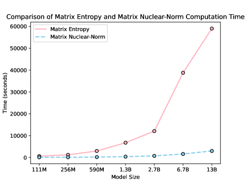
To evaluate the computational efficiency of Matrix Nuclear-Norm in comparison to Matrix Entropy for LLMs, we conducted experiments across various model sizes using multiple benchmark datasets. The results, summarized in Table 1, demonstrate a clear advantage of Matrix Nuclear-Norm in terms of computation time, particularly for larger models.
As model sizes increased, Matrix Entropy’s computation time rose dramatically, reaching approximately 16.3 hours for the 13B model . In contrast, Matrix Nuclear-Norm only required about 0.82 hours for the same model, representing nearly a 20-fold reduction in computation time. This trend was consistent across all model sizes, with Matrix Nuclear-Norm consistently proving to be much faster (as illustrated in Figure 1). For example, the 111M model showed that Matrix Nuclear-Norm was 8.58 times quicker than Matrix Entropy.
The significant efficiency gain is attributed to the lower computational complexity of Matrix Nuclear-Norm, , compared to Matrix Entropy’s . This makes Matrix Nuclear-Norm not only an effective but also a highly efficient metric for evaluating LLMs, especially as models continue to scale in size.
In summary, Matrix Nuclear-Norm achieves comparable evaluation accuracy to Matrix Entropy but with vastly superior computational efficiency, making it a practical and scalable choice for assessing LLMs.
| Model Size | Matrix Entropy Time (s) | Matrix Nuclear-Norm Time (s) | Ratio |
|---|---|---|---|
| 111M | 623.5367 | 72.6734 | 8.5800 |
| 256M | 1213.0604 | 110.8692 | 10.9414 |
| 590M | 2959.6949 | 184.7785 | 16.0175 |
| 1.3B | 6760.1893 | 379.0093 | 17.8365 |
| 2.7B | 12083.7105 | 732.6385 | 16.4934 |
| 6.7B | 38791.2035 | 1598.4151 | 24.2685 |
| 13B | 59028.4483 | 2984.1529 | 19.7806 |
5.2.2 Scaling Law of Matrix Nuclear-Norm
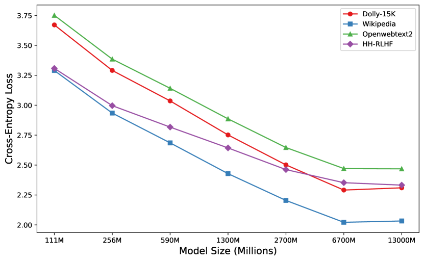
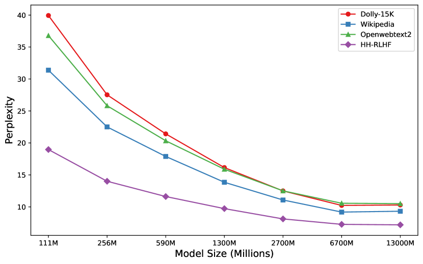
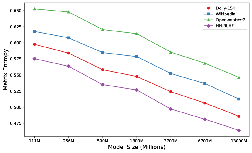
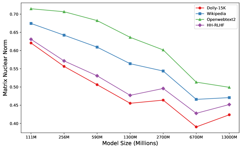
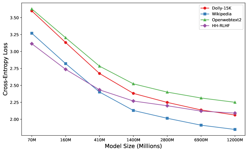
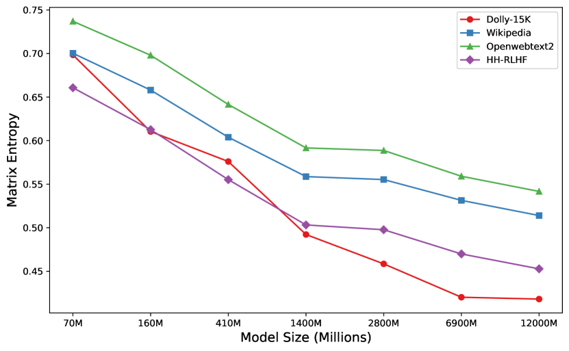
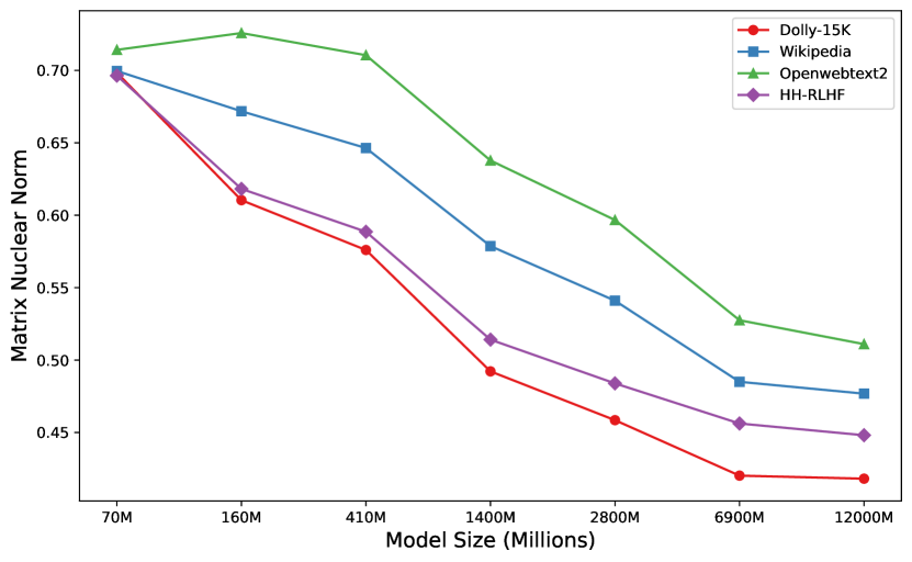
To affirm Matrix Nuclear-Norm’s efficacy as an evaluative metric, we evaluated Cerebras-GPT models on four datasets including dolly-15k, Wikipedia, openwebtext2, and hh-rlhf comparing Matrix Nuclear-Norm, matrix entropy, perplexity, and loss. Results, detailed in Table 11 (Appendix), demonstrate Matrix Nuclear-Norm’s consistent decrease with model size enlargement, signifying better data compression and information processing in larger models. This trend (see in Figure 2(d)) validates Matrix Nuclear-Norm’s utility across the evaluated datasets. Notably, anomalies at the 2.7B and 13B highlight areas needing further exploration.
5.2.3 Relationship of Benchmark INDICATORS
Findings indicate the efficacy of the Matrix Nuclear-Norm as a metric for evaluating LLM, as shown in Table 10 (Appendix), there is an overall downward trend in Matrix Nuclear-Norm values with increasing model sizes, signifying enhanced compression efficiency. However, notable anomalies at the 2.7B and 13B checkpoints suggest that these specific model sizes warrant closer examination. Despite these discrepancies, the Matrix Nuclear-Norm consistently demonstrates superior computational efficiency and accuracy compared to traditional metrics, highlighting its promising applicability for future model evaluations.
5.3 Language Investigation
5.3.1 Sentence Operation Experiments
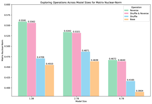
Figure 3 clearly indicates that sentence manipulations significantly influence Matrix Nuclear-Norm values, which generally decline as model size increases. This trend confirms the enhanced information compression capabilities of larger models. The ranking of Matrix Nuclear-Norm values by operation is as follows: Reverse Shuffle & Reverse Shuffle Base. This indicates that disrupting sentence structure through Reverse and Shuffle & Reverse operations leads to higher Matrix Nuclear-Norm values due to increased information chaos and processing complexity. In contrast, the Shuffle operation has minimal effect on compression, while the Base condition consistently yields the lowest Matrix Nuclear-Norm values, signifying optimal information compression efficiency with unaltered sentences.
Despite the overall downward trend in Matrix Nuclear-Norm values with increasing model size, the 2.7B model exhibits slightly higher values for Shuffle and Base operations compared to the 1.3B model. This anomaly suggests that the 2.7B model may retain more nuanced information when handling shuffled data or operate through more intricate mechanisms. However, this does not detract from the overarching conclusion that larger models excel at compressing information, thereby demonstrating superior processing capabilities.
5.3.2 Analysis of Length Dynamics
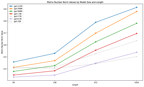
The analysis reveals that Matrix Nuclear-Norm values generally increase as input length rises, aligning with our expectations (see Figure 4). Longer inputs necessitate that the model manage and compress more information, which naturally leads to higher Matrix Nuclear-Norm values. Most models exhibit this trend, indicating effective handling of the increased information load.
However, the gpt-2.7B and gpt-13B models display anomalies in their Matrix Nuclear-Norm values at 64 and 128 tokens, where the value at 128 tokens is lower than that at 64 tokens. This discrepancy may be attributed to these models employing different information compression mechanisms or optimization strategies tailored to specific input lengths, allowing for more effective compression at those lengths.
Overall, aside from a few outliers, the results largely conform to expectations, demonstrating that Matrix Nuclear-Norm values increase with input length, reflecting the greater volume and complexity of information that models must handle.
To address the observed trend of rising Matrix Nuclear-Norm values with longer sentences, we incorporated a normalization step in our methodology via dividing the Matrix Nuclear-Norm values by the sentence length. This adjustment helps mitigate any biases introduced by models that tend to generate longer sentences during inference.
| GPT MODEL SIZE | |||||||
|---|---|---|---|---|---|---|---|
| LENGTH | 111M | 256M | 590M | 1.3B | 2.7B | 6.7B | 13B |
| 64 | 0.4574 | 0.4125 | 0.3787 | 0.3486 | 0.4053 | 0.3315 | 0.4148 |
| 128 | 0.5293 | 0.4680 | 0.4270 | 0.3835 | 0.4143 | 0.3477 | 0.4032 |
| 512 | 0.7883 | 0.6978 | 0.6251 | 0.5554 | 0.5265 | 0.4468 | 0.4422 |
| 1024 | 0.9132 | 0.8787 | 0.7802 | 0.6953 | 0.6351 | 0.5383 | 0.5028 |
5.3.3 Analysis of Prompt Learning
The experimental results (shown in Table 3) indicate that we performed inference on different sizes of GPT models using three carefully selected prompts (shown in Table 13) and calculated the Matrix Nuclear-Norm values of their responses. As the model size increased, the Matrix Nuclear-Norm values gradually decreased, demonstrating that larger models possess greater information compression capabilities. The prompts significantly influenced Matrix Nuclear-Norm, with variations reflecting the models’ responses to prompt complexity. Specifically, GPT-1.3B showed a notable decrease in Matrix Nuclear-Norm after the input prompts, indicating its sensitivity to them, while GPT-2.7B exhibited smaller changes. In contrast, GPT-6.7B displayed minimal variation across all prompts, suggesting stable performance regardless of prompt detail. Overall, more detailed prompts resulted in larger information volumes in the model’s responses, leading to corresponding changes in Matrix Nuclear-Norm values.
| ADDING PROMPT TO QA PAIRS | ||||||
|---|---|---|---|---|---|---|
| MODELS | EMPTY PROMPT | PROMPT 1 | PROMPT 2 | PROMPT 3 | AVERAGE | |
| CEREBRAS-GPT-1.3B | 0.150955 | 0.147577 | 0.140511 | 0.141358 | 0.14453 | ↓0.006425 |
| CEREBRAS-GPT-2.7B | 0.150130 | 0.151522 | 0.142834 | 0.151842 | 0.14844 | ↓0.001690 |
| CEREBRAS-GPT-6.7B | 0.132042 | 0.128346 | 0.124094 | 0.133211 | 0.12923 | ↓0.002812 |
6 Implementing Proposed Metrics: Evaluating and Ranking Language Models in Practice
6.1 Inference-Based Model Assessment
In this section, we evaluated model inference across the AlpacaEval and Chatbot Arena benchmarks using the Matrix Nuclear-Norm metric prior to the final MLP classification head. The analysis revealed that Matrix Nuclear-Norm reliably ranks model performance, with lower values indicating enhanced information processing efficiency, particularly as model size scales up.
For instance, the Llama-3 70B model demonstrated superior compression capabilities compared to its 8B counterpart, as reflected by significantly lower Matrix Nuclear-Norm values across both benchmarks (see Table A.2 in the Appendix). A similar trend was observed in the Vicuna family, where Matrix Nuclear-Norm values consistently decreased from 0.4623 for the 7B model to 0.3643 for the 33B model on the AlpacaEval dataset, indicating progressive improvements in information handling (see Table 4). Additionally, the DeepSeek models exhibited a consistent decrease in Matrix Nuclear-Norm values as model size increased, further demonstrating the metric’s validity.
Overall, these results substantiate Matrix Nuclear-Norm as a robust and reliable tool for evaluating and ranking LLMs, demonstrating its capacity to capture critical aspects of model performance across diverse benchmarks.
| Model | DataSet | 7B | 13B | 33B |
|---|---|---|---|---|
| Vicuna | Alpaca | 0.4623 | 0.4159 | 0.3643 |
| Arena | 0.4824 | 0.4311 | 0.3734 |
| Model | DataSet | 1.3B | 6.7B | 7B |
|---|---|---|---|---|
| DeepSeek | Alpaca | 0.4882 | 0.3472 | 0.3352 |
| Arena | 0.5754 | 0.4175 | 0.4357 |
6.2 Matrix Nuclear-Norm Benchmarking: Ranking Mid-Sized Models
In this experimental section, we utilized Matrix Nuclear-Norm to evaluate the responses of LLMs, focusing on 7B and 70B variants. Notably, lower Matrix Nuclear-Norm values indicate more efficient information compression, serving as a robust indicator of model performance.
Among the 7B models, DeepSeek-7B exhibited the most efficient information processing with the lowest average Matrix Nuclear-Norm score of 0.3855 across Alpaca and Arena datasets (see Table 4). Gemma-7B followed closely with an average score of 0.3879, whereas QWEN 2-7B demonstrated less efficient compression with an average score of 0.5870. In contrast, the 70B models showed varied performance, with Llama 2-70B achieving the best average score of 0.3974, slightly outperforming Llama 3-70B (0.4951) and QWEN models, which scored around 0.5.
Interestingly, certain 7B models, like DeepSeek-7B and Gemma-7B, outperformed larger 70B models, underscoring that model efficiency is not solely determined by size. These results highlight that factors such as architecture, training methodology, and data complexity play crucial roles in information processing capabilities beyond scale.
| MODEL | Matrix Nuclear-Norm | Rank | ||
| Alpaca | Arena-Hard | Avg Score | ||
| DeepSeek-7B | 0.3352 | 0.4357 | 0.3855 | |
| Gemma-7B | 0.3759 | 0.3998 | 0.3879 | |
| Vicuna-7B | 0.4623 | 0.4824 | 0.4724 | |
| LLaMA 2-7B | 0.4648 | 0.5038 | 0.4843 | |
| QWEN 1.5-7B | 0.4866 | 0.5165 | 0.5016 | |
| Mistral-7B | 0.4980 | 0.5126 | 0.5053 | |
| QWEN 2-7B | 0.5989 | 0.5751 | 0.5870 | |
| QWEN 1.5-72B | 0.5291 | 0.5065 | 0.5178 | |
| QWEN 2-72B | 0.5261 | 0.4689 | 0.4975 | |
| Llama 3-70B | 0.4935 | 0.4967 | 0.4951 | |
| Llama 2-70B | 0.3862 | 0.4086 | 0.3974 | |
To validate the design rationale and robustness of the Matrix Nuclear-Norm, we conducted a series of ablation studies. Due to space constraints, detailed results are provided in A.1 (appendix) to maintain brevity in the main text. These experiments included evaluations across different model families, such as Cerebras-GPT and Pythia, as well as comparisons of various data sampling strategies.The results demonstrate that the Matrix Nuclear-Norm consistently performs well across different model scales and sampling variations. This not only confirms its applicability across diverse models but also verifies its stability and reliability in handling large-scale datasets. We also provide an ablation study in the appendix, further proving the method’s efficiency and accuracy in evaluating LLMs.
7 Conclusion
In conclusion, Matrix Nuclear-Norm stands out as a promising evaluation metric for LLMs, offering significant advantages in assessing information compression and redundancy elimination. Its key strengths include remarkable computational efficiency, greatly exceeding that of existing metrics like matrix entropy, along with exceptional stability across diverse datasets. Matrix Nuclear-Norm’s responsiveness to model performance under varying inputs emphasizes its ability to gauge not only performance but also the intricate adaptability of models. This metric marks a significant advancement in NLP, establishing a clear and effective framework for future research and development in the evaluation and optimization of language models.
8 Limitations
Although Matrix Nuclear-Norm performs well in evaluating the performance of LLMs, it still has some limitations. First, since Matrix Nuclear-Norm’s computation relies on the model’s hidden states, the evaluation results are sensitive to both the model architecture and the training process. As a result, under different model designs or training settings, especially for models like GPT-1.3B and GPT-2.7B, inconsistencies in Matrix Nuclear-Norm’s performance may arise, limiting its applicability across a wider range of models. Additionally, while Matrix Nuclear-Norm offers computational efficiency advantages over traditional methods, it may still face challenges with resource consumption when evaluating extremely large models. As model sizes continue to grow, further optimization of Matrix Nuclear-Norm’s computational efficiency and evaluation stability is required.
9 Ethics Statement
Our study adheres to strict ethical guidelines by utilizing only publicly available and open-source datasets. We ensured that all datasets used, such as dolly-15k, hh-rlhf, OpenBookQA, Winogrande, PIQA, AlpacaEval, and Chatbot Arena, are free from harmful, biased, or sensitive content. Additionally, careful curation was conducted to avoid toxic, inappropriate, or ethically problematic data, thereby ensuring the integrity and safety of our research. This commitment reflects our dedication to responsible AI research and the broader implications of using such data in language model development.
References
- Bahri et al. [2024] Yasaman Bahri, Ethan Dyer, Jared Kaplan, Jaehoon Lee, and Utkarsh Sharma. Explaining neural scaling laws. Proceedings of the National Academy of Sciences, 121(27):e2311878121, 2024.
- Bai et al. [2022] Yuntao Bai, Andy Jones, Kamal Ndousse, Amanda Askell, Anna Chen, Nova DasSarma, Dawn Drain, Stanislav Fort, Deep Ganguli, Tom Henighan, et al. Training a helpful and harmless assistant with reinforcement learning from human feedback. arXiv preprint arXiv:2204.05862, 2022.
- Biderman et al. [2023] Stella Biderman, Hailey Schoelkopf, Quentin Gregory Anthony, Herbie Bradley, Kyle O’Brien, Eric Hallahan, Mohammad Aflah Khan, Shivanshu Purohit, USVSN Sai Prashanth, Edward Raff, et al. Pythia: A suite for analyzing large language models across training and scaling. In International Conference on Machine Learning, pp. 2397–2430. PMLR, 2023.
- Bisk et al. [2020] Yonatan Bisk, Rowan Zellers, Jianfeng Gao, Yejin Choi, et al. Piqa: Reasoning about physical commonsense in natural language. In Proceedings of the AAAI conference on artificial intelligence, volume 34, pp. 7432–7439, 2020.
- Celikyilmaz et al. [2020] Asli Celikyilmaz, Elizabeth Clark, and Jianfeng Gao. Evaluation of text generation: A survey. arXiv preprint arXiv:2006.14799, 2020.
- Chang et al. [2024] Yupeng Chang, Xu Wang, Jindong Wang, Yuan Wu, Linyi Yang, Kaijie Zhu, Hao Chen, Xiaoyuan Yi, Cunxiang Wang, Yidong Wang, et al. A survey on evaluation of large language models. ACM Transactions on Intelligent Systems and Technology, 15(3):1–45, 2024.
- Chen et al. [2024a] Jun Chen, Yong Fang, Ashish Khisti, Ayfer Ozgur, Nir Shlezinger, and Chao Tian. Information compression in the ai era: Recent advances and future challenges. arXiv preprint arXiv:2406.10036, 2024a.
- Chen et al. [2024b] Zhikai Chen, Haitao Mao, Hang Li, Wei Jin, Hongzhi Wen, Xiaochi Wei, Shuaiqiang Wang, Dawei Yin, Wenqi Fan, Hui Liu, et al. Exploring the potential of large language models (llms) in learning on graphs. ACM SIGKDD Explorations Newsletter, 25(2):42–61, 2024b.
- Chiang et al. [2023] Wei-Lin Chiang, Zhuohan Li, Zi Lin, Ying Sheng, Zhanghao Wu, Hao Zhang, Lianmin Zheng, Siyuan Zhuang, Yonghao Zhuang, Joseph E Gonzalez, et al. Vicuna: An open-source chatbot impressing gpt-4 with 90%* chatgpt quality. See https://vicuna. lmsys. org (accessed 14 April 2023), 2(3):6, 2023.
- Chiang et al. [2024] Wei-Lin Chiang, Lianmin Zheng, Ying Sheng, Anastasios Nikolas Angelopoulos, Tianle Li, Dacheng Li, Hao Zhang, Banghua Zhu, Michael Jordan, Joseph E Gonzalez, et al. Chatbot arena: An open platform for evaluating llms by human preference, 2024. URL: https://arxiv. org/abs/2403.04132, 2024.
- Clark et al. [2022] Aidan Clark, Diego de Las Casas, Aurelia Guy, Arthur Mensch, Michela Paganini, Jordan Hoffmann, Bogdan Damoc, Blake Hechtman, Trevor Cai, Sebastian Borgeaud, et al. Unified scaling laws for routed language models. In International conference on machine learning, pp. 4057–4086. PMLR, 2022.
- Conover et al. [2023] Mike Conover, Matt Hayes, Ankit Mathur, Jianwei Xie, Jun Wan, Sam Shah, Ali Ghodsi, Patrick Wendell, Matei Zaharia, and Reynold Xin. Free dolly: Introducing the world’s first truly open instruction-tuned llm. Company Blog of Databricks, 2023.
- Delétang et al. [2023] Grégoire Delétang, Anian Ruoss, Paul-Ambroise Duquenne, Elliot Catt, Tim Genewein, Christopher Mattern, Jordi Grau-Moya, Li Kevin Wenliang, Matthew Aitchison, Laurent Orseau, et al. Language modeling is compression. arXiv preprint arXiv:2309.10668, 2023.
- Dey et al. [2023] Nolan Dey, Gurpreet Gosal, Hemant Khachane, William Marshall, Ribhu Pathria, Marvin Tom, Joel Hestness, et al. Cerebras-gpt: Open compute-optimal language models trained on the cerebras wafer-scale cluster. arXiv preprint arXiv:2304.03208, 2023.
- Dubey et al. [2024] Abhimanyu Dubey, Abhinav Jauhri, Abhinav Pandey, Abhishek Kadian, Ahmad Al-Dahle, Aiesha Letman, Akhil Mathur, Alan Schelten, Amy Yang, Angela Fan, et al. The llama 3 herd of models. arXiv preprint arXiv:2407.21783, 2024.
- Dubois et al. [2024] Yann Dubois, Balázs Galambosi, Percy Liang, and Tatsunori B Hashimoto. Length-controlled alpacaeval: A simple way to debias automatic evaluators. arXiv preprint arXiv:2404.04475, 2024.
- Fazel [2002] Maryam Fazel. Matrix rank minimization with applications. PhD thesis, PhD thesis, Stanford University, 2002.
- Foundation [2024] Foundation. Foundation. https://dumps.wikimedia.org, 2024. [Online; accessed 2024-09-27].
- Gao et al. [2020] Leo Gao, Stella Biderman, Sid Black, Laurence Golding, Travis Hoppe, Charles Foster, Jason Phang, Horace He, Anish Thite, Noa Nabeshima, et al. The pile: An 800gb dataset of diverse text for language modeling. arXiv preprint arXiv:2101.00027, 2020.
- Gemini et al. [2023] Gemini, Rohan Anil, Sebastian Borgeaud, Yonghui Wu, Jean-Baptiste Alayrac, Jiahui Yu, Radu Soricut, Johan Schalkwyk, Andrew M Dai, Anja Hauth, et al. Gemini: a family of highly capable multimodal models. arXiv preprint arXiv:2312.11805, 2023.
- GPT-4 Achiam et al. [2023] Josh GPT-4 Achiam, Steven Adler, Sandhini Agarwal, Lama Ahmad, Ilge Akkaya, Florencia Leoni Aleman, Diogo Almeida, Janko Altenschmidt, Sam Altman, Shyamal Anadkat, et al. Gpt-4 technical report. arXiv preprint arXiv:2303.08774, 2023.
- Guo et al. [2024] Daya Guo, Qihao Zhu, Dejian Yang, Zhenda Xie, Kai Dong, Wentao Zhang, Guanting Chen, Xiao Bi, Y. Wu, Y. K. Li, Fuli Luo, Yingfei Xiong, and Wenfeng Liang, 2024. URL https://arxiv.org/abs/2401.14196.
- Guo et al. [2015] Qiang Guo, Caiming Zhang, Yunfeng Zhang, and Hui Liu. An efficient svd-based method for image denoising. IEEE transactions on Circuits and Systems for Video Technology, 26(5):868–880, 2015.
- Hestness et al. [2017] Joel Hestness, Sharan Narang, Newsha Ardalani, Gregory Diamos, Heewoo Jun, Hassan Kianinejad, Md Mostofa Ali Patwary, Yang Yang, and Yanqi Zhou. Deep learning scaling is predictable, empirically. arXiv preprint arXiv:1712.00409, 2017.
- Hoffmann et al. [2022] Jordan Hoffmann, Sebastian Borgeaud, Arthur Mensch, Elena Buchatskaya, Trevor Cai, Eliza Rutherford, Diego de Las Casas, Lisa Anne Hendricks, Johannes Welbl, Aidan Clark, et al. Training compute-optimal large language models. arXiv preprint arXiv:2203.15556, 2022.
- Jiang et al. [2023] Albert Q Jiang, Alexandre Sablayrolles, Arthur Mensch, Chris Bamford, Devendra Singh Chaplot, Diego de las Casas, Florian Bressand, Gianna Lengyel, Guillaume Lample, Lucile Saulnier, et al. Mistral 7b. arXiv preprint arXiv:2310.06825, 2023.
- Kaplan et al. [2020] Jared Kaplan, Sam McCandlish, Tom Henighan, Tom B Brown, Benjamin Chess, Rewon Child, Scott Gray, Alec Radford, Jeffrey Wu, and Dario Amodei. Scaling laws for neural language models. arXiv preprint arXiv:2001.08361, 2020.
- Kung et al. [1983] Sun-Yuan Kung, K Si Arun, and DV Bhaskar Rao. State-space and singular-value decomposition-based approximation methods for the harmonic retrieval problem. JOSA, 73(12):1799–1811, 1983.
- Lian et al. [2023a] Long Lian, Boyi Li, Adam Yala, and Trevor Darrell. Llm-grounded diffusion: Enhancing prompt understanding of text-to-image diffusion models with large language models. arXiv preprint arXiv:2305.13655, 2023a.
- Lian et al. [2023b] W Lian, B Goodson, E Pentland, et al. Openorca: An open dataset of gpt augmented flan reasoning traces, 2023b.
- Lin [2004] Chin-Yew Lin. Rouge: A package for automatic evaluation of summaries. In Text summarization branches out, pp. 74–81, 2004.
- Liu et al. [2023] Junling Liu, Chao Liu, Peilin Zhou, Qichen Ye, Dading Chong, Kang Zhou, Yueqi Xie, Yuwei Cao, Shoujin Wang, Chenyu You, et al. Llmrec: Benchmarking large language models on recommendation task. arXiv preprint arXiv:2308.12241, 2023.
- Long et al. [2016] Mingsheng Long, Han Zhu, Jianmin Wang, and Michael I Jordan. Unsupervised domain adaptation with residual transfer networks. Advances in neural information processing systems, 29, 2016.
- Mihaylov et al. [2018] Todor Mihaylov, Peter Clark, Tushar Khot, and Ashish Sabharwal. Can a suit of armor conduct electricity? a new dataset for open book question answering. arXiv preprint arXiv:1809.02789, 2018.
- Neubig [2017] Graham Neubig. Neural machine translation and sequence-to-sequence models: A tutorial. arXiv preprint arXiv:1703.01619, 2017.
- Papineni et al. [2002] Kishore Papineni, Salim Roukos, Todd Ward, and Wei-Jing Zhu. Bleu: a method for automatic evaluation of machine translation. In Proceedings of the 40th annual meeting of the Association for Computational Linguistics, pp. 311–318, 2002.
- Sakaguchi et al. [2021] Keisuke Sakaguchi, Ronan Le Bras, Chandra Bhagavatula, and Yejin Choi. Winogrande: An adversarial winograd schema challenge at scale. Communications of the ACM, 64(9):99–106, 2021.
- Sasaki [2007] Yutaka Sasaki. The truth of the f-measure. Teach tutor mater, 2007.
- Saul et al. [2005] Lawrence K Saul, Yair Weiss, and Léon Bottou. Advances in neural information processing systems 17: proceedings of the 2004 conference, volume 17. MIT Press, 2005.
- Sawada et al. [2023] Tomohiro Sawada, Daniel Paleka, Alexander Havrilla, Pranav Tadepalli, Paula Vidas, Alexander Kranias, John J Nay, Kshitij Gupta, and Aran Komatsuzaki. Arb: Advanced reasoning benchmark for large language models. arXiv preprint arXiv:2307.13692, 2023.
- Shannon [1948] Claude Elwood Shannon. A mathematical theory of communication. The Bell system technical journal, 27(3):379–423, 1948.
- Skean et al. [2023] Oscar Skean, Jhoan Keider Hoyos Osorio, Austin J Brockmeier, and Luis Gonzalo Sanchez Giraldo. Dime: Maximizing mutual information by a difference of matrix-based entropies. arXiv preprint arXiv:2301.08164, 2023.
- Skylion007 [2019] Skylion007. OpenWebText Corpus. http://Skylion007.github.io/OpenWebTextCorpus, 2019. [Online; accessed 2024-09-27].
- Tan et al. [2023] Zhiquan Tan, Jingqin Yang, Weiran Huang, Yang Yuan, and Yifan Zhang. Information flow in self-supervised learning. arXiv preprint arXiv:2309.17281, 2023.
- Team et al. [2024] Gemma Team, Thomas Mesnard, Cassidy Hardin, Robert Dadashi, Surya Bhupatiraju, Shreya Pathak, Laurent Sifre, Morgane Rivière, Mihir Sanjay Kale, Juliette Love, et al. Gemma: Open models based on gemini research and technology. arXiv preprint arXiv:2403.08295, 2024.
- Tishby et al. [2000] Naftali Tishby, Fernando C Pereira, and William Bialek. The information bottleneck method. arXiv preprint physics/0004057, 2000.
- Touvron et al. [2023] Hugo Touvron, Thibaut Lavril, Gautier Izacard, Xavier Martinet, Marie-Anne Lachaux, Timothée Lacroix, Baptiste Rozière, Naman Goyal, Eric Hambro, Faisal Azhar, et al. Llama: Open and efficient foundation language models. arXiv preprint arXiv:2302.13971, 2023.
- Valmeekam et al. [2023] Chandra Shekhara Kaushik Valmeekam, Krishna Narayanan, Dileep Kalathil, Jean-Francois Chamberland, and Srinivas Shakkottai. Llmzip: Lossless text compression using large language models. arXiv preprint arXiv:2306.04050, 2023.
- Vu et al. [2019] Tuan-Hung Vu, Himalaya Jain, Maxime Bucher, Matthieu Cord, and Patrick Pérez. Advent: Adversarial entropy minimization for domain adaptation in semantic segmentation. In Proceedings of the IEEE/CVF conference on computer vision and pattern recognition, pp. 2517–2526, 2019.
- Wang et al. [2023] Boxin Wang, Weixin Chen, Hengzhi Pei, Chulin Xie, Mintong Kang, Chenhui Zhang, Chejian Xu, Zidi Xiong, Ritik Dutta, Rylan Schaeffer, et al. Decodingtrust: A comprehensive assessment of trustworthiness in gpt models. In NeurIPS, 2023.
- Wang et al. [2024] Wenhai Wang, Zhe Chen, Xiaokang Chen, Jiannan Wu, Xizhou Zhu, Gang Zeng, Ping Luo, Tong Lu, Jie Zhou, Yu Qiao, et al. Visionllm: Large language model is also an open-ended decoder for vision-centric tasks. Advances in Neural Information Processing Systems, 36, 2024.
- Wei et al. [2022] Jason Wei, Yi Tay, Rishi Bommasani, Colin Raffel, Barret Zoph, Sebastian Borgeaud, Dani Yogatama, Maarten Bosma, Denny Zhou, Donald Metzler, et al. Emergent abilities of large language models. arXiv preprint arXiv:2206.07682, 2022.
- Wei et al. [2024] Lai Wei, Zhiquan Tan, Chenghai Li, Jindong Wang, and Weiran Huang. Large language model evaluation via matrix entropy. arXiv preprint arXiv:2401.17139, 2024.
- Yang et al. [2024] An Yang, Baosong Yang, Binyuan Hui, Bo Zheng, Bowen Yu, Chang Zhou, Chengpeng Li, Chengyuan Li, Dayiheng Liu, Fei Huang, et al. Qwen2 technical report. arXiv preprint arXiv:2407.10671, 2024.
- Yang [2019] Zhilin Yang. Xlnet: Generalized autoregressive pretraining for language understanding. arXiv preprint arXiv:1906.08237, 2019.
- Zhang et al. [2022] Susan Zhang, Stephen Roller, Naman Goyal, Mikel Artetxe, Moya Chen, Shuohui Chen, Christopher Dewan, Mona Diab, Xian Li, Xi Victoria Lin, et al. Opt: Open pre-trained transformer language models. arXiv preprint arXiv:2205.01068, 2022.
- Zhang et al. [2024] Tianyi Zhang, Faisal Ladhak, Esin Durmus, Percy Liang, Kathleen McKeown, and Tatsunori B Hashimoto. Benchmarking large language models for news summarization. Transactions of the Association for Computational Linguistics, 12:39–57, 2024.
- Zhang [2015] Zhihua Zhang. The singular value decomposition, applications and beyond. arXiv preprint arXiv:1510.08532, 2015.
- Zhao et al. [2023] Wayne Xin Zhao, Kun Zhou, Junyi Li, Tianyi Tang, Xiaolei Wang, Yupeng Hou, Yingqian Min, Beichen Zhang, Junjie Zhang, Zican Dong, et al. A survey of large language models. arXiv preprint arXiv:2303.18223, 2023.
- Zheng et al. [2023] Lianmin Zheng, Wei-Lin Chiang, Ying Sheng, Siyuan Zhuang, Zhanghao Wu, Yonghao Zhuang, Zi Lin, Zhuohan Li, Dacheng Li, Eric Xing, et al. Judging llm-as-a-judge with mt-bench and chatbot arena. Advances in Neural Information Processing Systems, 36:46595–46623, 2023.
Appendix A Appendix
A.1 Ablation Study
To thoroughly validate the rationale behind our metric design, experimental framework, and the efficacy of Matrix Nuclear-Norm, we conducted a series of ablation studies.
A.1.1 Different Model Family
In addition to evaluating Matrix Nuclear-Norm within the Cerebras-GPT model series, we extended our experiments to the Pythia model family, which spans from 14M to 12B parameters and is trained on consistent public datasets. Utilizing the same datasets as described in Section 5.2.2, we computed matrix entropy, loss values, and Matrix Nuclear-Norm for these models. The empirical results (see Figure 5(c)) demonstrate that the Matrix Nuclear-Norm values for the Pythia models adhere to established scaling laws. However, we excluded metrics for the 14M, 31M, and 1B models due to notable deviations from the expected range, likely stemming from the inherent instability associated with smaller parameter sizes when tackling complex tasks. This further reinforces Matrix Nuclear-Norm as a robust metric for assessing model performance, underscoring its utility in the comparative analysis of LLMs.
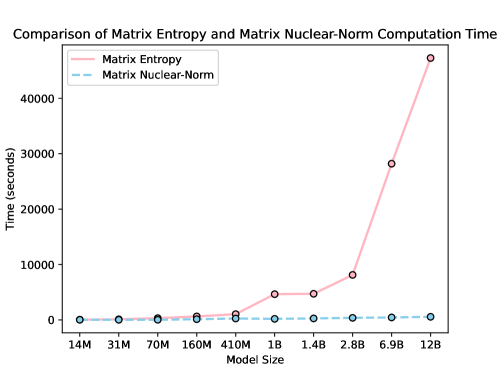
Moreover, we compared the computation times for Matrix Entropy and Matrix Nuclear-Norm across the Pythia models (can see in Figure 7). The results unequivocally indicate that Matrix Nuclear-Norm necessitates considerably less computation time than Matrix Entropy, underscoring its efficiency. Detailed results are summarized in Table 12.
A.1.2 Sampling Strategy
In the ablation experiments, we extracted a baseline subset of 10,000 entries from the extensive Wikipedia dataset using three random seeds to evaluate the robustness of the Matrix Nuclear-Norm metric. We also tested additional subsets of 15,000 and 20,000 entries due to potential entry count issues. Given the large scale of the datasets, comprehensive calculations were impractical, so we employed random sampling.
The results showed that variations in random seeds and sample sizes had minimal impact on Matrix Nuclear-Norm values, with a standard deviation of only 0.0004975 (see Table 6), indicating high consistency across trials. These findings confirm the Matrix Nuclear-Norm as a reliable metric for large-scale datasets, effectively evaluating information compression and redundancy elimination in LLMs.
| MODEL | SAMPLING STRATEGY | STANDARD DEVIATION | ||||
| 10000 (SEED 1) | 10000 (SEED 2) | 10000 (SEED 3) | 15000 | 20000 | ||
| CEREBRAS-GPT-1.3B | 0.5684 | 0.5670 | 0.5676 | 0.5699 | 0.5693 | 0.0004975 |
A.2 Supplementary Experiment Results
The following results provide additional insights into the Matrix Nuclear-Norm evaluations and comparisons across various language models:
- 1.
-
2.
Figure 6 illustrates that as model size increases, the computation time for Matrix Entropy grows exponentially, while Matrix Nuclear-Norm demonstrates a significant time advantage. This further emphasizes Matrix Nuclear-Norm’s efficiency in assessing model performance.The complete results are presented in Table 7, which includes all relevant time data for the Pythia model family.
- 3.
-
4.
Table 10 demonstrates the correlation between Matrix Nuclear-Norm and other benchmark indicators, showing a consistent trend where values decrease as model size increases. This analysis examines the performance of language modeling indicators across OpenBookQA, Winogrande, and PIQA datasets.
- 5.
-
6.
Table 13 shows the prompts used for the investigation of prompt learning.
| Model Size | Matrix Entropy Time (s) | Matrix Nuclear-Norm Time (s) | Ratio |
|---|---|---|---|
| 14M | 52.8669 | 22.2652 | 2.3772 |
| 31M | 114.0820 | 28.1842 | 4.0477 |
| 70M | 320.6641 | 24.3188 | 13.1855 |
| 160M | 631.9762 | 41.6187 | 15.1817 |
| 410M | 1040.9764 | 80.9814 | 12.8481 |
| 1B | 4650.1264 | 114.0639 | 40.8387 |
| 1.4B | 6387.0392 | 347.8670 | 18.3858 |
| 2.8B | 8127.1343 | 343.3888 | 23.6778 |
| 6.9B | 28197.8172 | 816.6332 | 34.5350 |
| 12B | 47273.5235 | 1276.1128 | 37.0485 |
| Model | DataSet | 0.5B | 1.5B | 7B | 72B |
|---|---|---|---|---|---|
| Alpaca | 0.6551 | 0.6176 | 0.5989 | 0.5261 | |
| QWEN 2 | Arena | 0.6872 | 0.6374 | 0.5751 | 0.4689 |
| Model | Data Set | 8B | 70B |
|---|---|---|---|
| Llama-3 | Alpaca | 0.5782 | 0.4935 |
| Arena | 0.5817 | 0.4967 |
| GPT MODEL SIZE | ||||||||
|---|---|---|---|---|---|---|---|---|
| BENCHMARKS | INDICATORS | 111M | 256M | 590M | 1.3B | 2.7B | 6.7B | 13B |
| ACCURACY | 0.118 | 0.158 | 0.158 | 0.166 | 0.206 | 0.238 | 0.286 | |
| MATRIX ENTROPY | 0.3575 | 0.3416 | 0.3237 | 0.3140 | 0.2991 | 0.2848 | 0.2767 | |
| LOSS | 5.6196 | 5.3536 | 5.1881 | 4.9690 | 4.8723 | 4.7195 | 4.7050 | |
| PPL | 148.38 | 108.10 | 83.45 | 65.10 | 50.93 | 41.80 | 40.89 | |
| OPENBOOKQA | MATRIX NUCLEAR-NORM | 0.4447 | 0.4057 | 0.3941 | 0.3644 | 0.4606 | 0.3672 | 0.4423 |
| ACCURACY | 0.488 | 0.511 | 0.498 | 0.521 | 0.559 | 0.602 | 0.646 | |
| MATRIX ENTROPY | 0.4073 | 0.3915 | 0.3706 | 0.3605 | 0.3419 | 0.3272 | 0.3149 | |
| LOSS | 4.7869 | 4.5854 | 4.4141 | 4.2513 | 4.1107 | 4.0109 | 4.0266 | |
| PPL | 39.81 | 30.25 | 26.57 | 21.87 | 18.55 | 16.53 | 16.94 | |
| WINOGRANDE | MATRIX NUCLEAR-NORM | 0.4802 | 0.4479 | 0.4440 | 0.4133 | 0.5232 | 0.4220 | 0.4964 |
| ACCURACY | 0.594 | 0.613 | 0.627 | 0.664 | 0.701 | 0.739 | 0.766 | |
| MATRIX ENTROPY | 0.4168 | 0.3991 | 0.3783 | 0.3676 | 0.3504 | 0.3344 | 0.3264 | |
| LOSS | 4.8425 | 4.5470 | 4.4029 | 4.1613 | 4.0075 | 3.8545 | 3.8826 | |
| PPL | 69.80 | 47.94 | 37.88 | 28.76 | 23.15 | 19.76 | 19.72 | |
| PIQA | MATRIX NUCLEAR-NORM | 0.4868 | 0.4327 | 0.4164 | 0.3826 | 0.4452 | 0.3675 | 0.4149 |
| DATASET | INDICATORS | GPT MODELS SIZE | ||||||
|---|---|---|---|---|---|---|---|---|
| 111M | 256M | 590M | 1.3B | 2.7B | 6.7B | 13B | ||
| DOLLY-15K | MATRIX ENTROPY | 0.5976 | 0.5840 | 0.5582 | 0.5477 | 0.5240 | 0.5064 | 0.4859 |
| LOSS | 3.6710 | 3.2907 | 3.0359 | 2.7517 | 2.5015 | 2.2911 | 2.3098 | |
| PPL | 39.93 | 27.53 | 21.42 | 16.15 | 12.50 | 10.23 | 10.30 | |
| MATRIX NUCLEAR-NORM | 0.6207 | 0.5565 | 0.5063 | 0.4553 | 0.4639 | 0.3904 | 0.4859 | |
| WIKIPEDIA | MATRIX ENTROPY | 0.6177 | 0.6077 | 0.5848 | 0.5786 | 0.5523 | 0.5368 | 0.5126 |
| LOSS | 3.2900 | 2.9343 | 2.6854 | 2.4282 | 2.2045 | 2.0216 | 2.0327 | |
| PPL | 31.38 | 22.51 | 17.89 | 13.85 | 11.08 | 9.19 | 9.32 | |
| MATRIX NUCLEAR-NORM | 0.6744 | 0.6422 | 0.6094 | 0.5639 | 0.5438 | 0.4660 | 0.4708 | |
| OPENWEBTEXT2 | MATRIX ENTROPY | 0.6527 | 0.6479 | 0.6206 | 0.6142 | 0.5855 | 0.5683 | 0.5463 |
| LOSS | 3.7509 | 3.3852 | 3.1414 | 2.8860 | 2.6465 | 2.4708 | 2.4685 | |
| PPL | 36.79 | 25.82 | 20.34 | 15.89 | 12.51 | 10.57 | 10.51 | |
| MATRIX NUCLEAR-NORM | 0.7147 | 0.7066 | 0.6823 | 0.6363 | 0.6017 | 0.5133 | 0.4991 | |
| HH-RLHF | MATRIX ENTROPY | 0.5753 | 0.5635 | 0.5350 | 0.5268 | 0.4971 | 0.4813 | 0.4640 |
| LOSS | 3.3078 | 2.9964 | 2.8171 | 2.6431 | 2.4622 | 2.3526 | 2.3323 | |
| PPL | 18.97 | 14.01 | 11.62 | 9.73 | 8.12 | 7.27 | 7.19 | |
| MATRIX NUCLEAR-NORM | 0.6309 | 0.5716 | 0.5307 | 0.4771 | 0.4959 | 0.4277 | 0.4518 | |
| PYTHIA MODELS SIZE | |||||||||||
|---|---|---|---|---|---|---|---|---|---|---|---|
| DATASETS | INDICATORS | 14M | 31M | 70M | 160M | 410M | 1B | 1.4B | 2.8B | 6.9B | 12B |
| MATRIX ENTROPY | 0.7732 | 0.7155 | 0.6707 | 0.6243 | 0.5760 | 0.5328 | 0.5309 | 0.5263 | 0.5003 | 0.4876 | |
| LOSS | 4.4546 | 4.0358 | 3.5990 | 3.1323 | 2.6752 | 2.4843 | 2.3816 | 2.2484 | 2.1368 | 2.0616 | |
| DOLLY-15K | MATRIX NUCLEAR-NORM | 0.7508 | 0.7735 | 0.6984 | 0.6104 | 0.5760 | 0.4710 | 0.4922 | 0.4585 | 0.4202 | 0.4181 |
| MATRIX ENTROPY | 0.7938 | 0.7442 | 0.7003 | 0.6580 | 0.6039 | 0.5584 | 0.5587 | 0.5553 | 0.5314 | 0.5140 | |
| LOSS | 4.1112 | 3.6921 | 3.2694 | 2.8207 | 2.4017 | 2.2213 | 2.1292 | 2.0140 | 1.9120 | 1.8489 | |
| WIKIPEDIA | MATRIX NUCLEAR-NORM | 0.6053 | 0.6700 | 0.6996 | 0.6718 | 0.6464 | 0.5591 | 0.5787 | 0.5410 | 0.4850 | 0.4768 |
| MATRIX ENTROPY | 0.8144 | 0.7749 | 0.7370 | 0.6980 | 0.6415 | 0.5944 | 0.5916 | 0.5887 | 0.5591 | 0.5417 | |
| LOSS | 4.3965 | 4.0033 | 3.6284 | 3.2031 | 2.7838 | 2.6198 | 2.5228 | 2.4005 | 2.3133 | 2.2502 | |
| OPENWEBTEXT2 | MATRIX NUCLEAR-NORM | 0.5041 | 0.6186 | 0.7142 | 0.7258 | 0.7105 | 0.6215 | 0.6378 | 0.5967 | 0.5275 | 0.5110 |
| MATRIX ENTROPY | 0.7673 | 0.7114 | 0.6607 | 0.6126 | 0.5552 | 0.5054 | 0.5032 | 0.4977 | 0.4699 | 0.4528 | |
| LOSS | 3.7466 | 3.4018 | 3.1146 | 2.7366 | 2.4340 | 2.3311 | 2.2687 | 2.1992 | 2.1199 | 2.0905 | |
| HH-RLHF | MATRIX NUCLEAR-NORM | 0.7353 | 0.7674 | 0.6964 | 0.6182 | 0.5886 | 0.4825 | 0.5141 | 0.4839 | 0.4562 | 0.4481 |
| Prompt ID | Prompt Content |
|---|---|
| Prompt 1 | You are an AI assistant. You will be given a task. You must generate a detailed and long answer. |
| Prompt 2 | You are a helpful assistant, who always provide explanation. Think like you are answering to a five year old. |
| Prompt 3 | You are an AI assistant. User will give you a task. Your goal is to complete the task as faithfully as you can. While performing the task think step-by-step and justify your steps. |
A.3 Analysis of Algorithmic Complexity
The primary computational expense of Matrix Nuclear-Norm arises from the calculation and sorting of the L2 norm of the matrix. By avoiding Singular Value Decomposition (SVD), we reduce the time complexity from the traditional nuclear norm of to , giving Matrix Nuclear-Norm a significant advantage in handling large-scale data. This reduction in complexity greatly enhances the algorithm’s practicality, especially for applications involving large matrices.
When analyzing the time complexity of the newly proposed Matrix Nuclear-Norm (L2-Norm Based Approximation of Nuclear Norm) against traditional Matrix Entropy, our objective is to demonstrate that Matrix Nuclear-Norm significantly outperforms Matrix Entropy in terms of time efficiency. We will support this claim with detailed complexity analysis and experimental results.
A.3.1 Time Complexity Analysis
Analysis 1: Time Complexity of Matrix Entropy
The computation of Matrix Entropy involves several complex steps, with the key bottleneck being Singular Value Decomposition (SVD), which is central to computing eigenvalues. The following steps primarily contribute to the time complexity:
-
1.
Matrix Normalization: This step has a time complexity of , where is the number of rows and is the number of columns.
-
2.
Computing the Inner Product Matrix: Calculating has a time complexity of due to the multiplication of two matrices sized .
-
3.
Singular Value Decomposition (SVD): The time complexity of SVD is , which is the primary computational bottleneck, especially for large .
Therefore, the total time complexity of Matrix Entropy can be approximated as:
This complexity indicates that Matrix Entropy becomes increasingly impractical for large-scale models as grows.
Analysis 2: Time Complexity of Matrix Nuclear-Norm
Matrix Nuclear-Norm avoids the SVD step by approximating the nuclear norm using the L2 norm, resulting in a more efficient computation. The analysis is as follows:
-
1.
Matrix Normalization: Similar to Matrix Entropy, this step has a time complexity of .
-
2.
Calculating the L2 Norm: For each column vector, the L2 norm is computed with a complexity of , where we take the square root of the sum of squares for each column vector.
-
3.
Sorting and Extracting the Top D Features: Sorting the L2 norms has a complexity of .
Therefore, the overall time complexity of Matrix Nuclear-Norm is:
This indicates that Matrix Nuclear-Norm is computationally more efficient, especially as increases.
A.3.2 Experimental Validation and Comparative Analysis
To empirically validate the theoretical time complexities, we conducted experiments using matrices of various sizes. Figure 6 shows that as increases, Matrix Nuclear-Norm consistently outperforms Matrix Entropy in terms of runtime, confirming the theoretical advantage.
Discussion of Assumptions and Applicability Our complexity analysis assumes , which holds in many real-world applications, such as evaluating square matrices in large-scale language models. However, in cases where , the time complexity might differ slightly. Nonetheless, Matrix Nuclear-Norm is expected to maintain its efficiency advantage due to its avoidance of the costly SVD operation.
Impact of Constant Factors Although both and indicate asymptotic behavior, Matrix Nuclear-Norm’s significantly smaller constant factors make it computationally favorable even for moderately sized matrices, as evidenced in our experimental results.
A.3.3 Conclusion of the Complexity Analysis
Through this detailed analysis and experimental validation, we conclude the following:
-
•
Matrix Entropy, with its reliance on SVD, has a time complexity of , making it computationally expensive for large-scale applications.
-
•
Matrix Nuclear-Norm, by using the L2 norm approximation, achieves a time complexity of , significantly reducing computational costs.
-
•
Experimental results confirm that Matrix Nuclear-Norm offers superior time efficiency for evaluating large-scale models, particularly those with millions or billions of parameters.
A.4 Proof of Theorem 1: Detailed Version
Here we present the proof of Theorem 1, demonstrating the strictly inverse monotonic relationship between and .
Given a matrix , where each element is non-negative and each row sums to 1, i.e.,
We define the Shannon entropy as:
and the Frobenius norm as:
Step 1: Analysis for a Fixed Row Vector
For a fixed row , let such that and . The entropy for this single row is given by:
and the Frobenius norm for this row vector is:
To determine when is maximized or minimized, we apply the method of Lagrange multipliers. Consider the function:
Taking partial derivatives with respect to and setting them to zero:
Since , we find for all . Thus, is maximized when all are equal. In this case,
Conversely, reaches its minimum when one element and all other . At this point,
This demonstrates that and are inversely related for each row.
Step 2: Inverse Monotonicity for the Entire Matrix
Since is the average of all values:
and is the square root of the sum of the squared norms for each row:
the inverse relationship between and implies that and are also inversely related across the entire matrix .
Step 3: Determining the Bounds of
To find the bounds, first note that when for all ,
which corresponds to the minimum discriminability.
For the upper bound, when each row has only one element equal to 1,
indicating maximum discriminability.
Step 4: Practical Implications
The inverse monotonic relationship between and is significant in machine learning and classification tasks, where maximizing implies achieving greater certainty in predictions. This property can be used to evaluate model performance, where higher corresponds to a model that is more confident and discriminative in its predictions. Therefore, and are strictly inversely monotonic, and the proof is complete.
A.5 Proof of Theorem 3
Given that is near , we want to approximate the -th largest singular value as . This approximation will be derived by examining the contributions of the columns of .
1. Decomposition of and Eigenvalues: By singular value decomposition (SVD), , where is a diagonal matrix containing singular values .
When looking at the product , the element at position is:
This sum represents the total squared magnitude of the entries in the -th column of .
2. Connecting to Singular Values: Since singular values represent the contribution of orthogonal projections of , if is near , the main contribution to the nuclear norm comes from columns with the largest sums of squared values .
3. Approximation: For matrices with well-distributed entries in each column (a common property when ), the top singular values can be effectively estimated by sorting these column norms. Hence, the largest singular values approximately correspond to the largest column norms .
Therefore, for each ,
This concludes the proof that the -th largest singular value can be approximated by the top values of column-wise norms of , as stated in Theorem 3.